extendingthecomputationalhorizon · 2015-06-29 · biology!math genome! permutations 5 3 9 4 2 1 8...
TRANSCRIPT

extending the computational horizon
Attila Egri-Nagy
Centre for Research and MathematicsSchool of Computing, Engineering and MathematicsUniversity of Western Sydney, Australia

research questions
∙ Bacterial Genomics (with Andrew Francis and VolkerGebhardt)∙ How to reconstruct phylogeny trees?
∙ Foundations of Computing (with James East, James D.Mitchell, Chrystopher L. Nehaniv).∙ What is computable with n states?∙ What is the structure of finite computations?
Precise answers can be obtained in abstract algebra, incomputational group and semigroup theory.
1

why computational?
∙ More examples, more raw data for the mathematicalreasoning.
2

bacterial changes
Single celled organisms with circular chromosome.
∙ Local changes such as single nucleotidepolymorphisms (SNPs):
ACGGCCCTTAGG −→ ACGGCCATTAGG
∙ Regional changes such as inversion that affect wholeregions along the chromosome.
1 2 3 4 5 6 1 2 6345
(Regional changes include inversion, translocation, deletion andothers.)
∙ Topological changes that produce knots and links inthe DNA. 3

biology→math
Genome→ permutations
5
3
9
42
1
8
7
6
Sequences of evolutionary→ Sequences of generators
Genomic distance→ Length of geodesic words
Genomic space→ Cayley-graph 4

1
2
3
45
6
7
8 1
2
3
-7-6
-5
-4
8
Reference genome and the signed permutation[1, 2, 3,−7,−6,−5,−4, 8].
5

where does the difficulty from?
∙ The groups are finite and well-studied (symmetric,hyperoctahedral), but big, e.g. S80
∙ The generating sets are unusual, “biological”.
For example,
∙ 2-inversions of the circular genome (vs. linear)∙ looking at the “width” as well
Strategy: Calculate and look at small, but non-trivialexamples to get insights.
6

symmetries of irreducible generating sets
1 Z2 Z2 × Z2 Z3 D8 S3 S4 S5S2 1S3 1 1S4 8 5 1S5 150 25 1 1 1S6 7931 645 11 6 4 20 2 2
7

abstract and transformation semigroups
DefinitionA semigroup is a set S withan associative binaryoperation S× S→ S.
Example (Flip-flop monoid)1 a b
1 1 a ba a a bb b a b
DefinitionA transformation semigroup(X, S) is a set of states X anda set S of transformationss : X → X closed underfunction composition.
Example (Transformations)
=
8

abstract and transformation semigroups
DefinitionA semigroup is a set S withan associative binaryoperation S× S→ S.
Example (Flip-flop monoid)1 a b
1 1 a ba a a bb b a b
DefinitionA transformation semigroup(X, S) is a set of states X anda set S of transformationss : X → X closed underfunction composition.
Example (Transformations)
=8

flip-flop, the 1-bit memory semigroup
write 0 write 1 read
[11] [22] [12]
So these are computational devices... ≈ automata
With transformation semigroups, we get all semigroups.(Cayley’s theorem)
9

degree 2 transformation semigroups
[11],[12],[21],[22]
[11],[12],[22]
[12],[22][11],[22] [11],[12] [12],[21]
[11][22] [12]
∅ 10

data flood
Number of subsemigroups of full transformationsemigroups.
#subsemigroups #conjugacy classes #isomorphism classesT0 1 1 1T1 2 2 2T2 10 8 7T3 1 299 283 267T4 3 161 965 550 132 069 776 131 852 491
After discounting the state-relabelling symmetries thedatabase of degree 4 transformation semigroups is stillaround 9GB.
11
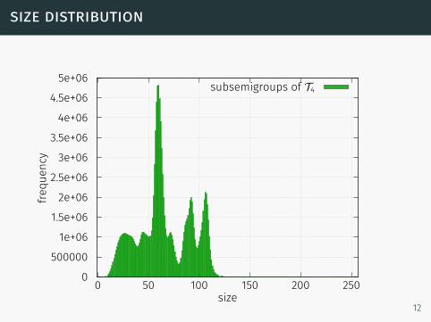
size distribution
0
500000
1e+06
1.5e+06
2e+06
2.5e+06
3e+06
3.5e+06
4e+06
4.5e+06
5e+06
0 50 100 150 200 250
frequency
size
subsemigroups of T4
12

size distribution – logarithmic scale
1
10
100
1000
10000
100000
1e+06
1e+07
0 50 100 150 200 250
frequency
size
subsemigroups of T4
13

diagram semigroups – typical elements
∈ PBn,
∈ Bn, ∈ Pn
∈ PTn, ∈ I∗n
14

diagram semigroups – typical elements
∈ In, ∈ Bn
∈ Tn, ∈ TLn
∈ Sn, 1n
15

diagram semigroups
P1 ↪→ T2P2 ↪→ T5
B1 ∼= T1B2 ↪→ T3
TL1 ∼= T1TL2 ↪→ T2TL3 ↪→ T4
P1 ↪→ B2
Tn In I∗n Bn
Sn1n
TLn
PTn
Bn
PBn
Pn
16

Order n = 1 n = 2 n = 3 n = 4 n = 5 n = 6PBn 2(2n)2 16 65536 236 264 2100 2144
Bn 2n2 2 16 512 65536 225 236
Pn B2n =∑2n
1 S(2n, k) 2 15 203 4140 115975 4213597PTn (n+ 1)n 2 9 64 625 7776 117649I∗n
∑n1 k!
(S(n, k)
)2 1 3 25 339 6721 179643Tn nn 1 4 27 256 3125 46656In
∑n0 k!
(nk)2 2 7 34 209 1546 13327
Bn (2n− 1)!! 1 3 15 105 945 10395Sn n! 1 2 6 24 120 720
TLn, Jn Cn = 1n+1
(2nn)
1 2 5 14 42 132
17

computational horizon
n = 1 n = 2 n = 3 n = 4 n = 5 n = 6PBn 1262Bn 4 385Pn 4 272PTn 4 50 94232In 4 23 2963I∗n 2 6 795Tn 2 8 283 132069776Bn 2 6 42 10411TLn 2 4 12 232 12592 324835618Sn 1 2 4 11 19 56
18

deeper into semigroup structure
Given a semigroup S, the equivalence relation J isdefined by
t J s ⇐⇒ S1tS1 = S1sS1,
where S1 is S with an identity adjoined in case S is not amonoid.
In other words,
t J s ⇐⇒ ∃p,q,u, v ∈ S1 such that t = psq and s = utv
The equivalence classes of J are “local pools ofreversibility”.
19

a = ( 1 2 3 4 52 2 1 2 4 ), b = ( 1 2 3 4 53 5 2 3 2 ), b = ( 1 2 3 4 53 5 4 5 4 ) andM = 〈a,b, c〉. |M| = 31
{1, 2, 3, 4, 5}1
{1, 2, 4}a
{2, 3, 5}b
{3, 4, 5}c
{1, 2, 4}ba
{1, 2, 4}ca
{2, 5} {2, 3} {4, 5}b2,b3 cb,bcb bc,b2c
{1, 4} {3, 5}caca cacaca ac
{2, 4}b2ab3a
{1, 2}bcbacba
{1, 4} {3, 5}baca bac
{1, 4} {3, 5}baba bababa ab
{1} {2} {3} {4} {5}ababa a2 abab abc a2c
20

transformation semigroups of degree 3
x axis : size of the semigroups
y axis : the number of D-classes
21

subsemigroups of the degree 5 jones monoid
x axis : size of the semigroups
y axis : the number of D-classes
22

inverse semigroups (of partial permutations)
x axis : size of the semigroups
y axis : the number of D-classes
23

transformation semigroups of degree 4
x axis : size of the semigroups
y axis : the number of D-classes
24

transformation semigroups of degree 4
x axis : size of the semigroups
y axis : the number of D-classes
25

even more structure, all green’s relations
L, R equivalence relations
t R s ⇐⇒ tS1 = sS1,t L s ⇐⇒ S1t = S1s,
t J s ⇐⇒ S1tS1 = S1sS1
L ◦ R = R ◦ L = D
J = D in the finite case
t R s ⇐⇒ ∃p,q ∈ S1 such that t = sp and s = tq
t L s ⇐⇒ ∃p,q ∈ S1 such that t = ps and s = qtt J s ⇐⇒ ∃p,q,u, v ∈ S1 such that t = psq and s = utv
26

“eggbox” picture
Tables are D-classes. Columns are L-classes, rows areR-classes. Shaded cells are H-classes that containidempotents – used for locating subgroups of thesemigroup. T3:
1
*
2
* *
* *
* *
3
*
*
*
27

temperley-lieb, jones monoid
Catalan numbers, sequences of well-formed parentheses.
corresponds to (()(()))()
Applications in Physics: statistical mechanics,percolation problem.
=
So the usual semigroup thing: look at the eggbox picture,locate the idempotents.
28

first glimpse through the usual eggbox diagrams
J9
29

top level
J16
30

level 2
31

level 3
32

level 4
33

level 5
34
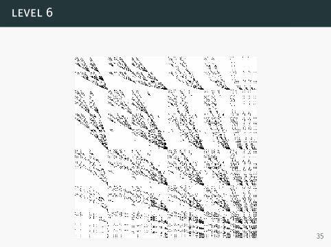
level 6
35

level 7
36

level 8
37

level 9
38

mathematics & computation
The Good We can discover/construct more and morenew, interesting and useful mathematics byusing computers.
The Bad There is a gap between mathematical rigourand the correctness of softwareimplementations and the physicality ofcomputation.
and The Ugly Developing software is still detrimental toacademic career.
39

