extended ls-svm for system modeling
TRANSCRIPT

PhD Thesis
EXTENDED LS-SVM FOR SYSTEM MODELING
József Valyon
Advisor: Gábor Horváth PhD
Budapest University of Technology and Economics
Department of Measurement and Information Systems

I express my thanks to the Department of Measurement and Information Systems of the Budapest University of Technology and Economics, Budapest, Hungary, for providing me with all the support necessary for completing this Thesis.
I gratefully thank to my supervisor Gábor Horváth PhD for directing and supporting my research from the very beginning for almost 7 years. His ideas, suggestions and encouragement were a great help in dealing with the many obstacles and small tasks that have finally lined up to provide the backbone of the main propositions. I give a special thank for the uncountable hours he spent with reading, correcting and rereading this work, which has improved a lot as a result.
I would like to thank my family, especially my wife for the constant support and motivation to complete this work.
This work was partly sponsored by National Fund for Scientific Research (OTKA)
under contract T 046771.

BME-MIT Extended LS-SVM for System Modeling
i
List of figures Figure 2.1. Illustration of the black-box modeling problem. 7
Figure 2.2. A static system that is made dynamic by delays (NARX). 11
Figure 2.3. Two possible separating hypersurfaces that separate the two classes with zero empirical risk.
Without further information it is impossible to decide for one of them. 12
Figure 2.4. An illustration of under- and overfitting. The simple linear function (solid line) underfits the data
making training errors. The complex one (dash-dotted line) has no training error but may not perform well on
unseen data (bad generalization ability). The function with intermediate complexity (dashed line) is probably
the best decision boundary, by being simple, but yet not too bad on the data. 13
Figure 2.5. The consistency of the ERM principle. 15
Figure 2.6. An example demonstrating the capacity of a linear separation. Three points –in two dimensions- are
always separable (a.,b.), but four points are not (c.). 17
Figure 2.7. Schematic illustration showing the expected risk in relation to VC dimension and other error
measures. 18
Figure 3.1. The geometric interpretation of the distance to the hyperplane in two dimensions. 23
Figure 3.2. The use of slack variables to describe the “error” of a sample. a.) The sample falls on the rights side
of the optimal separation surface (dotted line), but it is inside the margin. b.) The data sample is not classified
correctly. 25
Figure 3.3. The primal, the feature, the kernel space and the mappings between. 27
Figure 3.4. The ε–insensitive loss function (a), and the resulting insensitivity zone (b). We also demonstrate an
error at a sample marked by ξ . 30
Figure 3.5. The different chunking strategies. The thin line represents the sample set, while the thick line
shows, the actual working set. Three iterations are illustrated. 32
Figure 3.6. Illustration of the misclassification error and the complexity of the separation surface. a.) Allowing
misclassifications in the feature space means a lower feature space dimensionality and a simple separation
surface in the primal space. b.) A perfect separation in the feature space correspond to a complex surface in
the primal space. 33
Figure 3.7. Illustration of sparseness, based on using a subset of the samples. 36
Figure 3.8. Illustration of the sorted kα spectrum. 37
Figure 3.9. Four stages of the pruning algorithm. 38
Figure 3.10. The neural interpretation of a Support Vector Machine. 40
Figure 3.11. The ε –insensitive loss function (a), and the squared loss function (b). 41
Figure 4.1. A kernel space based on two SVs ( 2=M ) and the output. The black dots represent the training
samples, while the white dot illustrates how the output is determined in the recall phase. 43
Figure 4.2. The image of training samples in a kernel space of different dimensions. Using all three samples as
support vectors (kernel centers), a three-dimensional kernel space guarantees exact fit for the samples. The
dashed lines represent a zone in which errors can be accepted (corresponding to the ε -insensitivity of SVM).
45
Figure 4.3. The calculation of the Ω matrix. The gray background illustrates, which elements are affected by
omitting a row and/or a column corresponding to an input vector. 46
Figure 4.4. An illustration of the “by-design” error term introduced through regularization. 55
Figure 4.5. Illustration of the matrix operations involved in the a.) training, b.) testing and c.) evaluating. 56
Figure 4.6. Illustration of information loss in case of full reduction The effect of regularization is also illustrated.
For the dotted line a larger regularization (smaller C ) is used. 58
Figure 4.7. Constructing a vector as a linear combination. 60
BME-MIT Extended LS-SVM for System Modeling
ii
Figure 4.8. An intermediate step of the Gaussian elimination with partial pivoting (the ip elements are the
delegates to become the next pivot element). 61
Figure 4.9. Illustration of the sorted kα spectrum and the different pruning strategies . 62
Figure 4.10. Four stages of the inverse pruning algorithm. 62
Figure 4.11. The effects of pruning and inverse pruning. 63
Figure 4.12. The least squares and the robust (bisquare) fitting in two dimensions. 71
Figure 4.13. Linear interpolation and incremental learning. 72
Figure 4.14. A nonlinear solution in the kernel space, based on two SVs ( 2=M ) one output. The black dots
represent the training samples, while the white dot illustrates how the output is determined in the recall phase.
73
Figure 5.1. The different reduction methods plotted together. 78
Figure 5.2. A partially reduced LS–SVM, where the support vectors were selected by the proposed method
(tolerance= 0.2). 78
Figure 5.3. The RREF method distributes the kernel centers correctly, even if the data samples are not
distributed evenly (tolerance= 0.001). 79
Figure 5.4. Approximation of a two-dimensional sinc function. a.) The plotted training samples and b.) the
result of the partially reduced LS–SVM, where the support vectors were selected by the proposed method. The
SVs are marked with black dots. 80
Figure 5.5. The comparison of the pruning algorithms for different regularization constants. 82
Figure 5.6. The result of the traditional LS-SVM pruning and the inverse LS-SVM pruning (MSEpruning=0.0061,
MSEinverse_pruning=0.0023). 83
Figure 5.7. The result of the traditional LS-SVM pruning and the inverse LS-SVM pruning in case of two outliers
(MSEpruning=0.0102, MSEinverse_pruning=0.0015). 83
Figure 5.8. The box plot summarizing the MSE for 30 experiments utilizing the five different selection methods.
Figure b.) is the same, but it omits the inverse pruning, which is much worst than the other methods. 85
Figure 5.9. The classification boundaries obtained for the standard LS–SVM a.) and the LS2–SVM b.). 89
Figure 5.10. The predicted values and the errors for the Mackey-Glass prediction problem. a.) The results for
the traditional LS–SVM b.) the result of LS–SVM with traditional pruning c.) the result for the proposed
methods. The pruned, and the LS2-SVM results contain only 68 support vectors. 90
Figure 5.11. The continuous black line plots the result for a partially reduced LS-SVM solved by the bisquare
weights method. (MSEbisquare-SVM= 1.89*10-3, MSELS-SVM= 6.86*10-2). 91
Figure 5.12. The continuous black line plots the result for a partially reduced LS-SVM solved by the least
trimmed squares method. (MSELTS-SVM= 3.42*10-3, MSELS-SVM= 6.86*10-2) 92
Figure 6.1. The grey dashed line is the original LS-SVM’s result, while the continuous black line plots the result
for the proposed method. 94
Figure 6.2. The continuous black line plots the result for a generalized LS-SVM using 20 evenly distributed ic
kernel centers. The dashed line is the original LS-SVM. 95
Figure 7.1. Photo of an LD steel converter. 97
Figure 7.2. The main steps of the steel making process. a.) The solid waste iron is filled. b.) The molten pig
iron is loaded. c.) Blasting with oxygen. d.) Additives are supplemented. e.) Quality testing. f.) Steel is tapped
off. 98
Figure 7.3. The temperature (forward) and the oxygen (inverse) model 100
Figure 7.4. The misclassification error rate plotted for different combinations of C and σ . The best settings
are at the minimum of these surfaces. a.) LS-SVM , b.) LS2-SVM. 104
BME-MIT Extended LS-SVM for System Modeling
iii
Figure 7.5. The misclassification error rate of the original not pruned LS-SVM plotted for different values of C
and σ . The other parameter is fixed at the optimum a.) 3 =σ , b.) 100 C = 105
Figure 7.6. The misclassification error rate of the LS2-SVM plotted for different values of C and σ . The other
parameter is fixed at the optimum a.) 3.7 =σ , b.) 500 C = . The tolerance is 0.01. 106
Figure 7.7. The misclassification error rate of the LS-SVM plotted for different combinations of C and σ . a.)
the error surface based on 3000 training samples, b.) the difference between the 1000 and 3000 training
sample based error surfaces. 106
Figure 7.8. The misclassification error rate of the LS2-SVM plotted for different combinations of C and σ . a.)
the error surface based on 3000 training samples, b.) the difference between the 1000 and 3000 training
sample based error surfaces. 107
Figure 7.9. The dependence of the misclassification rate and the number of support vectors from the tolerance
value. 108
Figure 7.10. Illustration of a Gaussian kernel matrix from the viewpoint of σ . The kernel matrix of a sinc
represented by 40 training samples is plotted a.) 2=σ ,b.) 6=σ . 109
Figure 10.1. Box plot for an example distribution. The inter quartile range (IQR) is the distance between the
75th percentile and the 25th percentile. The IQR is essentially the range of the middle 50% of the data.
Because it uses the middle 50%, the IQR is not affected by outliers or extreme values. The IQR is also equal to
the length of the box in a box plot. 118
Figure 10.2. An example matrix for a.) Row Echelon Form, b.) Reduced Row Echelon Form. 123
BME-MIT Extended LS-SVM for System Modeling
iv
List of tables Table 1.1. List of symbols and notations ................................................................................................. vi
Table 3.1. The most common kernel functions. ....................................................................................... 28
Table 3.2. The equations for calculating the estimate for an input. ............................................................ 39
Table 3.3. The neural network interpretation of the LS–SVM. .................................................................... 40
Table 3.4. The comparison of the basic methods. .................................................................................... 42
Table 4.1. The comparison of the different reduction methods. ................................................................. 67
Table 5.1. The number of support vectors, and the mean squared error (MSE) calculated for different training
set sizes of the same problem using the proposed methods (the tolerance was set to 0.25).. ....................... 79
Table 5.2. Inverse pruning vs. traditional pruning for different sample sizes, SV number and iterations (130
samples reduced to 32, 100000=C ). ............................................................................................... 82
Table 5.3. The mean squared errors calculated for different selection methods. .......................................... 86
Table 5.4. The average of 10 MSE calculated for the different selection methods at different C and tolerance (
ε ′ ) parameter settings. ...................................................................................................................... 86
Table 5.5. The mean squared errors calculated for the different methods. .................................................. 88
Table 5.6. Errors for the Mackey-Glass problem calculated for different network sizes. ................................ 88
Table 5.7. Results achieved for benchmark problems. Where NTR is the number of training inputs and NTS is
the number of test samples. The NLS-SVM and NLS2-SVM columns contain the network size of the solutions
respectively. The hit/miss classification rates are also shown for both methods the test sets. ....................... 89
Table 5.8. Errors for the Mackey-Glass problem calculated for different network sizes. ................................. 91
Table 7.1. The LD converter dataset contains the data of three campaigns. .............................................. 102
Table 7.2. The normalized LD converter datasets used in the experiments. .............................................. 102
Table 7.3. Experimental setups used in the LD steel making problem. ..................................................... 103
Table 7.4. The estimates for σ and C based on 1000 training samples. ................................................ 105
Table 7.5. An illustration on the dependence of SV number on the σ value ( 01.0=′ε ). ........................ 109
Table 7.6. The results achieved for LD converter modeling problem, using different models. The tolerance used
in the reduction is moderate, thus the number of support vectors is reduced greatly, but a fairly good
performance is obtained. ................................................................................................................... 110
Table 7.7. The results achieved for LD converter modeling problem, using different models. The tolerance used
in the reduction is small, thus there are more support vectors kept for a better performance. .................... 110
Table 7.8. The results achieved for LD converter modeling problem, using different models. In this case the
tolerance is too large, resulting in a very few SVs and consequently unacceptable large errors. .................. 111
Table 7.9. The results achieved for a corrupted LD converter modeling dataset, using different models. The
tolerance used for reduction is moderate: 01.0=′ε . ........................................................................... 111
Table 7.10. The results achieved for a corrupted LD converter modeling dataset, using different models. The
tolerance used for reduction is small: 005.0=′ε . ............................................................................... 112
Table 10.1. Estimated impact of the different choices made during the modeling. ..................................... 126
Table 10.2. The most important converter parameters collected during production. ................................... 127
BME-MIT Extended LS-SVM for System Modeling
v
Abbreviations CG Conjugate Gradient
EIV Errors In Variables (method)
ERM Empirical Risk Minimization
FVS Feature Vector Selection
GSVM Generalized Support Vector Machines
KKT Karush–Kuhn–Tucker (conditions)
KRR Kernel Ridge Regression
IQR Interquartile Range
SMO Sequential Minimal Optimization
SOR Successive overrelaxation
SRM Structural Risk Minimization
SSVM Smooth Support Vector Machines
SVM Support Vector Machines
SVC Support Vector Classification
SVR Support Vector Regression
SV Support Vector
QP Quadratic Programming
LAR Least Absolute Residuals
LD Linz-Donawitz (converter)
LS-SVM Least Squares Support Vector Machines
LS2-SVM Least Squares - Least Squares Support Vector Machines
LTS Least Trimmed Squares
MSE Mean Square Error
NARMAX Non-Linear Auto-Regressive Moving Average with Exogeneous Input
NARX Non-Linear Autoregressive Model Structure with Exogeneous Input
NBJ Nonlinear Box Jenkins Model
NFIR Non-Linear Finite Inpulse Response Model
NN Neural Network
NOE Non-Linear Output Error Model
PCA Principal Component Analysis
RBF Radial Basis Function (network)
RE LS-SVM Robust Extended LS-SVM
RR Ridge Regression
RREF Reduced Row Echelon Form
RRKRR Reduced Rank Kernel Ridge Regression
RSVM Reduced Support Vector Machines
UCI University of California, Irvine
VC Vapnik- Chervonenkis (dimenzió)

BME-MIT Extended LS-SVM for System Modeling
vi
Notations In this work we are determined to always use the most common, well-known notations of the literature. Since there are both common mathematical methods and special intelligent system related algorithms described, the original notaitions of the fields –due to the many different sources- are quite different. For the intelligent methods presented, we will try to use one consistent notation, therefore it may differ from the original referred literature.
When the common mathematical background is discussed we use the common mathematical notations, but when they are applied as part of a method, it is substituted according to the context. The two discussions are well separated throughout this work, so the actual notation will always be clear from the context and the actual meaning of all symbols will always be defined.
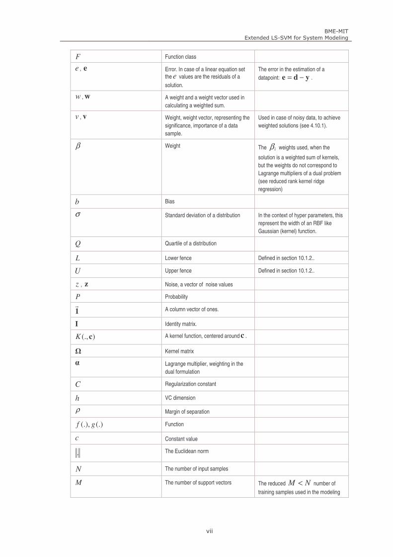
The following table (Table 1.1.) describes the most commonly used symbols and their meanings:
Table 1.1. List of symbols and notations
INTELLIGENT SYSTEMS
SYMBOL MEANING COMMENT
Χ input space
Υ output space
x input vector
d desired (true system) output
y estimated (predicted) output
i , j , k Indices used to enumerate elements of
vectors, data sets etc. In case of dynamic problems k is also
used to represent discrete time steps.
ℜ Real numbers
nℜ Euclidean space with n dimensions
S A set of data samples The set off all the collected input output
values available.
trainS Training set A subset of all data samples ( S ) used
for training. The train index is usually
omitted for simplicity, when the
meaning is clear from the context.
testS Test set A subset of all data samples ( S ) used
for testing. The test index is usually
omitted for simplicity, when the
meaning is clear from the context.
l Loss This value represents the cost of
deviating from a desired value. The loss
is calculated according to a loss
function.
(.)L Loss function This function provides the loss ( l ) in a
given situation. L is usually a function
of the desired and the estimated output.
R Risk (true risk)
empR Empirical risk
BME-MIT Extended LS-SVM for System Modeling
vii
F Function class
e , e Error. In case of a linear equation set
the e values are the residuals of a
solution.
The error in the estimation of a
datapoint: yde −= .
w , w A weight and a weight vector used in
calculating a weighted sum.
v , v Weight, weight vector, representing the
significance, importance of a data
sample.
Used in case of noisy data, to achieve
weighted solutions (see 4.10.1).
β Weight The iβ weights used, when the
solution is a weighted sum of kernels,
but the weights do not correspond to
Lagrange multipliers of a dual problem
(see reduced rank kernel ridge
regression)
b Bias
σ Standard deviation of a distribution In the context of hyper parameters, this
represent the width of an RBF like
Gaussian (kernel) function.
Q Quartile of a distribution
L Lower fence Defined in section 10.1.2..
U Upper fence Defined in section 10.1.2..
z , z Noise, a vector of noise values
P Probability
1r
A column vector of ones.
I Identity matrix.
)(.,cK A kernel function, centered around c .
Ω Kernel matrix
α Lagrange multiplier, weighting in the
dual formulation
C Regularization constant
h VC dimension
ρ Margin of separation
(.)(.), gf Function
c Constant value
. The Euclidean norm
N The number of input samples
M The number of support vectors The reduced NM < number of
training samples used in the modeling
BME-MIT Extended LS-SVM for System Modeling
viii
ξ Slack variable
(.)J Cost function Usually an index is used to indicate the
method whose cost function is defined.
(.)L Lagrangian
(.)O Ordo notation
p Pivot element The pivot element used in Gauss-
Jordan elimination
ε A small constant, usually representing
a tolerable error value.
In case of the ε -insenstitive loss
function, this hyper parameter defines
the maximum error value that can be
ignored.
ε ′ Tolerance value used in the RREF
method.
qp, The input and the feature space
dimensionality respectively.
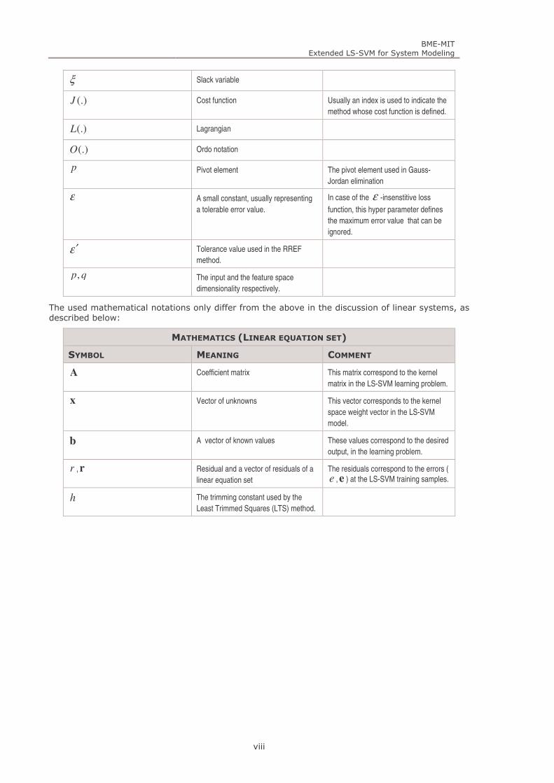
The used mathematical notations only differ from the above in the discussion of linear systems, as described below:
MATHEMATICS (LINEAR EQUATION SET)
SYMBOL MEANING COMMENT
A Coefficient matrix This matrix correspond to the kernel
matrix in the LS-SVM learning problem.
x Vector of unknowns This vector corresponds to the kernel
space weight vector in the LS-SVM
model.
b A vector of known values These values correspond to the desired
output, in the learning problem.
r , r Residual and a vector of residuals of a
linear equation set
The residuals correspond to the errors (
e , e ) at the LS-SVM training samples.
h The trimming constant used by the
Least Trimmed Squares (LTS) method.
BME-MIT
Extended LS-SVM for System Modeling
1
Table of contents 1. INTRODUCTION ...................................................................................................................................... 3
2. LEARNING FROM SAMPLES ............................................................................................................... 7
2.1. PROBLEM FORMULATIONS ......................................................................................................................... 9
2.2. DYNAMIC PROBLEMS ................................................................................................................................. 9
2.2.1. Creating a data set for dynamic problems ...................................................................................... 10
2.3. GENERALIZATION (INDUCTIVE PRINCIPLES) ............................................................................................ 12
2.3.1. Cross-validation .............................................................................................................................. 13
2.3.2. Regularization ................................................................................................................................. 14
2.3.3. Statistical learning theory ............................................................................................................... 14
2.4. REMARKS ON STATISTICAL LEARNING .................................................................................................... 18
3. KERNEL METHODS ............................................................................................................................. 21
3.1. SUPPORT VECTOR MACHINES ................................................................................................................. 21
3.1.1. Linearly separable classification (margin maximization) ............................................................... 21
3.1.2. Linearly non-separable classification ............................................................................................. 25
3.1.3. Kernel trick ...................................................................................................................................... 26
3.1.4. Nonlinear Support Vector classifier ................................................................................................ 28
3.1.5. Support Vector Regression .............................................................................................................. 29
3.1.6. Fast SVM solutions .......................................................................................................................... 31
3.1.7. Remarks on SVM ............................................................................................................................. 33
3.2. LEAST SQUARES SUPPORT VECTOR MACHINES ....................................................................................... 33
3.2.1. LS-SVM regression .......................................................................................................................... 34
3.2.2. LS-SVM classification ..................................................................................................................... 35
3.2.3. Sparse LS-SVM ................................................................................................................................ 36
3.2.4. Large Scale LS-SVM ........................................................................................................................ 38
3.2.5. Remarks on LS-SVM ........................................................................................................................ 39
3.3. DISCUSSION ON KERNEL METHODS .......................................................................................................... 39
3.3.1. The neural network interpretation of support vector solutions ....................................................... 39
3.3.2. Comparison of the methods ............................................................................................................. 41
3.3.3. Goals and exclusions ....................................................................................................................... 42
4. EXTENDED LEAST SQUARES SUPPORT VECTOR MACHINES ............................................... 43
4.1. REDUCTION METHODS ............................................................................................................................. 45
4.1.1. The kernel regularized LS-SVM ...................................................................................................... 50
4.1.2. The least-squares solution (LS2-SVM) ............................................................................................. 51
4.1.3. Sparseness and performance ........................................................................................................... 52
4.2. RELATED WORKS CONCERNING REDUCTION ............................................................................................ 53
4.2.1. Reduced Support Vector Machines .................................................................................................. 53
4.2.2. Reduced Rank Kernel Ridge Regression ......................................................................................... 53
4.3. DISCUSSION ON REDUCTION METHODS .................................................................................................... 54
4.4. REMARKS ON REDUCTION ........................................................................................................................ 58
4.5. SUPPORT VECTOR SELECTION ................................................................................................................. 59
4.5.1. The RREF method for SV selection ................................................................................................. 59
4.5.2. Inverse LS-SVM pruning ................................................................................................................. 61
4.5.3. Fixed Size Reduced LS-SVM............................................................................................................ 63
4.6. RELATED WORKS CONCERNING SUPPORT VECTOR SELECTION ................................................................. 64
4.6.1. Fixed Size LS-SVM .......................................................................................................................... 64
4.6.2. The Feature Vector Selection (FVS) algorithm for RRKRR ............................................................ 64
4.6.3. Pruning, inverse pruning and FVS for SV selection in extended LS-SVM....................................... 65
4.7. DISCUSSION ON SELECTION METHODS ..................................................................................................... 66
4.8. REMARKS ON SELECTION METHODS ........................................................................................................ 68
4.9. SOLVING THE OVERDETERMINED SYSTEM - ROBUST SOLUTIONS ............................................................. 69
4.9.1. Weighted methods ............................................................................................................................ 69
4.9.2. Robust methods ................................................................................................................................ 71
4.9.3. Locally linear and nonlinear fitting in kernel space ........................................................................ 71
4.10. RELATED WORKS CONCERNING ROBUST SOLUTIONS ............................................................................ 73
4.10.1. Weighted LS-SVM ........................................................................................................................ 73
BME-MIT
Extended LS-SVM for System Modeling
2
4.11. REMARKS ON ROBUST SOLUTIONS ....................................................................................................... 74
5. EXPERIMENTS ...................................................................................................................................... 77
5.1. USING PARTIAL REDUCTION .................................................................................................................... 77
5.2. SELECTION METHODS ............................................................................................................................. 78
5.2.1. The automatic (RREF) selection method ........................................................................................ 78
5.2.2. Inverse pruning ............................................................................................................................... 80
5.2.3. Comparison of selection methods ................................................................................................... 84
5.3. COMPARISON OF LS-SVM SOLUTIONS ................................................................................................... 87
5.3.1. Classification .................................................................................................................................. 88
5.3.2. Dynamic problems/Time series prediction ...................................................................................... 89
5.4. ROBUST METHODS .................................................................................................................................. 91
6. OTHER LS-SVM EXTENSIONS .......................................................................................................... 93
6.1. OUTLIER DETECTION ............................................................................................................................... 93
6.2. GENERALIZED LS-SVM FORMULATION .................................................................................................. 94
7. INDUSTRIAL SYSTEM MODELING – A STEELMAKING PROCESS ........................................ 97
7.1. BACKGROUND ........................................................................................................................................ 97
7.2. THE PROBLEM DESCRIPTION ................................................................................................................... 98
7.3. MODELING APPROACH ............................................................................................................................ 99
7.4. THE NEURAL MODEL OF THE LD CONVERTER PROJECT ......................................................................... 100
7.5. VALIDATION METHOD ........................................................................................................................... 101
7.6. EXPERIMENTS ....................................................................................................................................... 102
7.6.1. Hyperparameter selection ............................................................................................................. 104
7.6.2. Support vector selection ................................................................................................................ 107
7.6.3. Results ........................................................................................................................................... 110
8. SUMMARY OF NEW SCIENTIFIC RESULTS ................................................................................ 113
9. CONCLUSIONS, FUTURE RESEARCH........................................................................................... 115
10. APPENDIX ............................................................................................................................................ 116
10.1. PROPERTIES OF DATASETS ................................................................................................................. 116
10.1.1. Noisy data .................................................................................................................................. 116
10.1.2. Outliers ...................................................................................................................................... 117
10.1.3. Causes of outliers ...................................................................................................................... 118
10.2. APPROXIMATION ............................................................................................................................... 118
10.2.1. Least-squares approximation (linear regression) ..................................................................... 119
10.2.2. Weighted approximation ........................................................................................................... 120
10.2.3. Regularization ........................................................................................................................... 120
10.2.4. Tikhonov regularization ............................................................................................................ 120
10.3. RIDGE REGRESSION ........................................................................................................................... 121
10.3.1. Linear Ridge Regression ........................................................................................................... 121
10.3.2. Kernel Ridge Regression ........................................................................................................... 122
10.3.3. Remarks on Ridge Regression ................................................................................................... 122
10.4. REDUCED ROW ECHELON FORM (RREF) .......................................................................................... 123
10.5. ITERATIVE SOLUTION TO LS-SVM .................................................................................................... 124
10.6. STEELMAKING DATABASE ................................................................................................................. 125
10.6.1. Database characteristics ........................................................................................................... 125
10.6.2. The parameters describing the LD converter ............................................................................ 127
11. REFERENCES ...................................................................................................................................... 129
1. Introduction BME-MIT
Extended LS-SVM for System Modeling
3
1. INTRODUCTION
System modeling is an important way of investigating and understanding the world around. There are several different ways of building system models, utilizing different forms of knowledge about the system, and applying different modeling approaches, methods [1].
In most cases the only knowledge available is some measured input and output data. When only input–output observations are obtained, a behavioral or a black-box model can be constructed. This Thesis is concerned with some of the most important aspects of black-box system modeling [2].
The primary aims are to:
provide a good quality model based on the observed data.
reduce model complexity, namely to find a small, compact model of the problem.
handle the effects of noise corrupting the sample data.
reduce the algorithmic complexity of model construction.
There are many other questions concerning system modeling that are not addressed here (e.g. parameter selection, using prior information etc.). A more detailed description on the scope of this Thesis and on the issues not dealt with will be given in section 3.3.3.
Learning from data
In system modeling the primary goal is to give a good representation of the system, which means that the model should reproduce the output for a certain input as close as possible (in the sense of a predefined error measure). In order to do this by black-box modeling, the input-output relation represented by the system should be described –as good as possible- through the samples used in training, thus the number and the quality of the data is extremely important. The available dataset may be problematic in many ways (noisy samples, too small or too large datasets, non uniformly distributed or missing samples etc.).
From the viewpoint of the primary aims, this work will focus on probably the two most typical problems concerning the sample data, namely the size of the dataset and the noise corrupting the samples. The number and the quality of the data samples have many effects concerning our goals. In the context of this work, the size of the dataset is considered from two aspects: (1) the problem, (2) the model and its construction. First of all, the dataset –utilized for constructing the model- should be large enough to describe the problem, moreover if noise is present, it should contain enough data to statistically reduce the effect of noise. On the other hand, the size of the dataset can affect both the algorithmic complexity of the model construction and the complexity of the model.
The size of the dataset may lead to the following problems:
A small dataset may not contain sufficient information to describe the problem, therefore the model cannot be precise. Although there are methods to reduce the effect of this problem, this can only be done to a certain limited extent, and due to the missing information there is quite little that can be done. This problem is mentioned because the industrial process described in this Thesis is very underrepresented by the data.
Due to a large dataset, the model construction may be algorithmically complex. The size of the dataset effects both the memory and time requirements of the model construction method, which grows along with the number of samples.
1. Introduction BME-MIT
Extended LS-SVM for System Modeling
4
The resulting model may be too complex. This means that after construction – in the recall phase – it requires many computations to calculate an estimate and its implementation is harder.
The main problem is that – even in case of a representative dataset – the problems addressed are ill posed [3]-[5]. One only knows a set of input-output samples which is by far not enough to describe the problem, since usually there may be infinitely many solutions that fulfill the constraints represented by the samples. There is a need for some other criteria or constraint that supports the construction of the model by providing supplementary knowledge – supporting the choice form the possible solutions – besides the pure sample dataset. This principle is used to achieve a result that provides acceptable answer for the inputs not contained in the training data. The ability to estimate outputs for yet unseen inputs is called generalization. To create a model with good generalization capability one needs ways to control this property. There are two different approaches to this problem:
By splitting the available sample set into a training and test dataset. The model is built using the training dataset, while its generalization capability is validated by testing it on the test dataset. The most common method based on this idea is cross-validation.
By using a training method that incorporates additional knowledge, such as theoretical results to achieve a solution that generalizes well. Some of these solutions can provide a guaranteed upper bound on the generalization error.
Unfortunately the training data is often corrupted by noise, which –if not handled properly– misleads the training, therefore a method used for such a modeling task must offer some solutions to reduce or eliminate this effect. In a real-life system modeling problem one is almost always faced with the problem of imprecise data. According to the nature of the distortions usually three cases are handled:
Gaussian noise.
Outliers.
Known noise properties (e.g. distributions, noise variances).
According to the discussion above, the dataset used poses many problems that should be handled by the applied modeling approach.
Modeling approaches
In black-box system modeling, the use of intelligent systems, soft computing methods and more specifically Neural Networks (NN) are an important and therefore widely used alternative [1],[2]. Thus neural networks play a very important role in system modeling, which is especially true if model building relies mainly on observed data.
The most important questions concerning neural networks are about
their modeling capabilities: what kind of input–output relations can be implemented using the given model, and
their generalization capabilities: what are the answers of a trained network for inputs not used during training.
The main reason for the importance of neural networks comes from their general modeling capabilities. Some of the neural network architectures (e.g. multi-layer perceptrons, MLPs [6],[7]), or Radial Basis Function (RBF) networks) are proven to be universal approximators [6]-[8], which means that an MLP or an RBF of proper size can approximate any continuous function arbitrarily well. A neural network is trained using a finite number of training examples and the goal is that the network should give correct responses for inputs not used during training, thus it should generalize well to unseen samples. To achieve a good generalization with a NN a good training method (e.g. free from being stuck in a local minimum and using a good stopping criterion) should be used, which can mostly be based on trial and error or heuristic methods.
In the past decade, new approaches of learning machine construction, the Support Vector Machines (SVM) [9],[10],[3] and their least squares modification, the Least Squares Support Vector Machine (LS–SVM) [11]-[14] have been introduced and are gaining more and more attention, because they incorporate some useful features that make them favorable in handling the most common modeling situations.
1. Introduction BME-MIT
Extended LS-SVM for System Modeling
5
From the viewpoint of model construction, the advantage is that the support vector methods eliminate certain crucial questions required by neural network construction and training. For example, the network structure, like the number of neurons (and some properties of neurons e.g. activation function), the training method, its parameters or the stopping criteria and a number of related decisions are eliminated. Instead of these questions the support vector machines require a few parameters (about 2-3, depending on the method and kernel used) and apply an analytic learning method.
The SVM includes an additional principle to provide good generalization. In the case of SVM this extra principle is the Structural Risk Minimization (SRM) principle [3], which aims at achieving a simple model, thus one that corresponds to a smooth solution. This principle is derived from the classification problem, where the primary focus is to maximize the margin, thus the distance between the separation hyperplane and the separated classes.
This concludes to the primary advantage of SVM, namely that this model guaranties an upper bound on the generalization error. Another important advantage of the traditional SVM is its sparseness, meaning that the method selects some input vectors as support vectors and bases its model on these vectors (hence the name). These vectors are considered to be the most important ones concerning the problem. The use of only a subset of all vectors is a desirable property of SVM, because it provides additional information regarding the training data, and concludes in a more effective solution formulating a smaller model.
The LS-SVM was introduced to overcome the high computational complexity (both time and space) of SVM based model construction. LS-SVM training requires the solution of a linear equation set, while the standard SVM involves a long and computationally hard quadratic programming problem. The method effectively reduces the algorithmic complexity, however for really large problems, comprising a very large number of training samples, even this least-squares solution can become highly memory and time consuming. Although many iterative solutions have been proposed to overcome these algorithmic issues [15]-[20], these problems should still be addressed.
On the other hand, the price paid for this algorithmic gain is that sparseness is lost, resulting in a much higher model complexity. The least squares version incorporates all training data in the model. The sparseness of traditional SVM [21] can also be reached with LS–SVM by applying a pruning method [22]-[25]. Pruning techniques are also well known in the context of traditional neural networks [26]. Their purpose is to reduce the complexity of the networks by eliminating as much hidden neurons as possible. Unfortunately if the traditional LS–SVM pruning method is applied, the performance may decline as training samples are eliminated, since the information (input-output relation) they described is lost. Another problem is that this iterative method multiplies the algorithmic complexity.
The LS–SVM method should also be able to handle outliers (e.g. resulting from non–Gaussian noise). Another modification of the method, called weighted LS–SVM [27], is aimed at reducing the effects of this type of noise. The biggest problem is that pruning and weighting – although their goals do not rule out each other – cannot be used at the same time, because they work in opposition.
The main task, namely to model a complex industrial process, involving large datasets leads to the use of LS-SVM mainly due to computational issues. Since the available LS-SVM solution does not meet all demands, it must be extended to tackle these drawbacks. In order to achieve our main goals based on LS-SVM, the following must be done:
A sparse LS-SVM model must be constructed.
The new modeling approach must be robust against noise.
The extended LS-SVM should keep the computational complexity in mind, and if possible it should be further reduced.
The quality of the model must be maintained, despite the modifications required.
1. Introduction BME-MIT
Extended LS-SVM for System Modeling
6
The outline of this Thesis is as follows:
Outline
This Thesis is organized into five logical parts (described below) comprising 13 major sections. Part 1 and 2 describes the theoretical backgrounds of the propositions. The third and fourth part contains the contributions of this work. In part 5 an industrial problem is solved by applying the proposed methods. The detailed outline of this Thesis is as follows:
I. Background
1. In section 2 the basic black-box modeling problem is described, along with the most common related problems.
2. The second part (section 3) summarizes the basic kernel methods including the traditional SVM (section 3.1) and LS-SVM (section 3.2). Section 3.3 contains some discussion on the traditional support vector methods and concludes to the goals of this Thesis.
II. Contributions
3. The third part contains the major contributions of the present work by describing the major extensions applied to the LS-SVM model (section 4). The propositions together form a framework to reach a sparse and robust LS-SVM, which is referred to as Extended LS-SVM. First a special reduction method is presented (summarized by Thesis 1), named partial reduction, which is the key to achieve a sparse solution (section 4.1). In order to reduce the original LS-SVM problem, an SV selection method must be introduced (covered by Thesis 2), to provide grounds for the reduction, by determining a subset of the training samples to serve as support vectors in the model (section 4.5). Since the proposed partial reduction leads to an overdetermined problem, there are several ways to find an optimal linear (or even a non-linear) solution (summarized in Thesis 3), especially in case of noisy data. The possible solutions, including robust methods, are described in section 4.9. To justify the results, some experiments are presented in section 5. This part contains artificial, “toy” problems and benchmark problems, to demonstrate the strength of the proposed methods.
4. After the main results (section 6), some other related methods are proposed. These methods fit in the framework of the Extended LS-SVM but have not been included in the major statements, because these results are not directly connected to the primal theoretical context of the extended LS-SVM. The experiments concerning these propositions are also presented here in this section.
III. Industrial application
5. The proposed Extended LS-SVM methods have also been applied to a real-life complex industrial problem, namely to the problem of steelmaking with the use of a Linz-Donawitz (LD) converter [28]. This problem motivated the research towards the propositions, because it generated many problems, when traditional SV methods were applied. Previously this problem had been solved with a neural model, but now the Extended LS-SVM is applied (section 7).
The ideas presented, cover many aspects of the Extended LS-SVM, but many open questions remain. Section 8 summarizes the main statements. Section 9 contains the conclusions, and also defines the most important open questions and research areas that are not covered here.
Section 10 contains the Appendix, while section 11 lists the references used in this Thesis.
2. Learning from samples BME-MIT
Extended LS-SVM for System Modeling
7
2. LEARNING FROM SAMPLES
The main objective of learning is to describe an unknown dependency, represented by a data set, which is collected through measurements of our system. The measured values can usually be categorized as being an input or an output. In most of the cases the valid ranges of the input values (input domains) are known and can be used as the possible inputs for our system. On the other hand, the output data are only available for certain inputs. These samples are the data examples representing the problem.
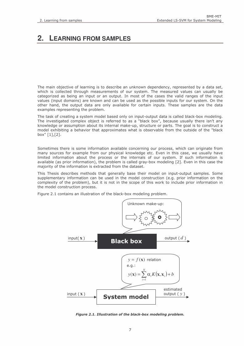
The task of creating a system model based only on input-output data is called black-box modeling. The investigated complex object is referred to as a “black box”, because usually there isn’t any knowledge or assumption about its internal make-up, structure or parts. The goal is to construct a model exhibiting a behavior that approximates what is observable from the outside of the "black box" [1],[2].
Sometimes there is some information available concerning our process, which can originate from many sources for example from our physical knowledge etc. Even in this case, we usually have limited information about the process or the internals of our system. If such information is available (as prior information), the problem is called gray-box modeling [2]. Even in this case the majority of the information is extracted from the dataset.
This Thesis describes methods that generally base their model on input-output samples. Some supplementary information can be used in the model construction (e.g. prior information on the complexity of the problem), but it is not in the scope of this work to include prior information in the model construction process.
Figure 2.1 contains an illustration of the black-box modeling problem.
Figure 2.1. Illustration of the black-box modeling problem.
Unknown make-up:
Black box input(x ) output ( d )
)(xfy = relation
e.g.:
( ) bKy i
N
i
i +α=∑=
xxx ,)(1
System model input (x )
estimated output ( y )

2. Learning from samples BME-MIT
Extended LS-SVM for System Modeling
8
The purpose of estimating the dependency between the input and output variables is to be able to determine the values of output variables for any input. Depending on the number of inputs and the number of outputs four different cases can be distinguished:
SISO – Single Input Single Output
SIMO – Single Input Multiple Output
MISO – Multiple Input Single Output
MIMO – Multiple Input Multiple Output
but the implementation of these problems can all be derived from a MISO model, therefore (if not stated otherwise) the discussion is limited to this class of problems, without loosing generality.
Let Χ and Υ denote input and the output space respectively. Given the Χx ∈i input vectors and
the corresponding Υ∈id output variables ( Ni ,...,1= ), the full set of sample data is
NidS ii ,...,1),( =Υ×∈= Χx ,
where N is the number of all available data. The measured output d represents the true output of the system; therefore it is often referred to as the desired value. Throughout this work, the known output of a system (the outputs provided by the sample dataset), and the predicted output (the outputs predicted by a model) will be distinguished by a different notation using:
d for the true system output ( Υ∈d ),
y for the predicted output ( Υ∈y ).
There are two major types of tasks discussed in this Thesis:
Classification – the output variable(s) takes discrete values, often called labels or class
labels. ( 1,1−=y )
Regression – the output variable(s) takes real number values ( ℜ∈y ).
For the purposes of building (training) and then validating (testing) a model the data samples are usually split into two subsets:
Training samples – The set of known input-output data couples used in training the model (train
S ).
Test samples – A subset of the data samples used for testing the quality of the trained
model ( testS ).
The ),( ii dx data samples are assumed to be drawn identically and independently from ),( ΥΧP ,
which is an unknown but fixed probability distribution over the space Υ×Χ .
The relationship between the input and the output variables is an Υ→Χ:f function. To decide,
which of the many possible functions describes best the dependency observed in the training sample, the concept of a loss function L is introduced:
ℜ→Υ×Υ:L . (2.1)
The loss function defines the cost of the predicted value’s ( )( ii fy x= ) deviation from the true
value. The loss ( il ) calculated for the ie error value
)( iii fde x−= , (2.2)
)),(()( iiii dfLeLl x== (2.3)
describes the cost of the error in estimating id for the i
x input.
2. Learning from samples BME-MIT
Extended LS-SVM for System Modeling
9
Our f function should minimize the risk functional defined as
( ) ddPdfLfR dd),(),()( xxx∫= (2.4)
wherein unfortunately the ( )dP ,x joint probability density function is not known. Under certain
conditions, defined in [3],[4] )( fR may be estimated by an empirical risk functional:
( )∑=
=N
i
iiemp dfLN
fR1
),(1
)( x (2.5)
For this, the following three steps are necessary. First, a class of functions F needs to be defined. Second, a suitable loss L is to be fixed. Finally, a method has to be provided to find the function
Ff ∈ which minimizes the risk [ ]fRemp .
2.1. Problem formulations
According to the above described data set specification, this section defines the specific problem formulations. In both cases the input and output may be disturbed by some noise or the dataset may contain errors (e.g. outliers).
Classification
A data set N
iii
traind
1,
==Ζ x is obtained, where
Pi R∈x represents a P-dimensional input vector
and 1,1−∈id is the scalar target output (desired class).
In case of noise, the data set becomes: N
iiiitrain
d 1, =∗+=Ζ zx , where
Pi R∈z is the noise
corrupting the input and ∗id represent the output which may indicate the wrong class.
Regression
A data set N
iiitrain
d 1, ==Ζ x is obtained, where P
i R∈x represents a p-dimensional input vector
and Rdi ∈ is the scalar target output (desired response).
In case of noise the data set becomes: N
i
o
iiii
trainzd
1,
=++=Ζ zx , where
Pi R∈z and Rz
o
i ∈
stand for the input- and the output noise respectively..
For the sake of simplicity I do not formally include the additive noise when such a problem is described, but it is always stated if the samples (input and/or output) should be considered noisy. These notations are used only in case the amounts of noise added to the input and output samples are considered in the discussion.
2.2. Dynamic problems
Most of the real life systems are dynamic, where the output depends not only on the inputs, but the current state – resulting from past events - of the system. In this case it is assumed, that the response of the system depends on the previous inputs, outputs and/or on the system state, thus the system has a memory (e.g. it contains feedback connections). This case can also be handled as a regression (function approximation), but the input variables are extended to include earlier inputs and/or outputs [1],[2].
A special kind of dynamic problem that should be mentioned is the time series prediction problem, which is very common in the field of industrial system modeling. Time series prediction is the use of a model to predict future events based on known past events. This means that the input and output data must have an ordering and the model constructed should represent the timely dynamics of the process. This problem can be generalized, since the prediction may be done along any variable (not only the time), but in a time series prediction problem a series of output values
2. Learning from samples BME-MIT
Extended LS-SVM for System Modeling
10
changing in time must be predicted, based on some earlier values and sometimes some other inputs.
Since most of the basic modeling tools –that are simple, thus easy to handle – are originally static (for example SVMs), there is a need to extend these systems to handle dynamic problems as well. The following method shows a very simple way to extend the capabilities of static support vector models to handle dynamic problems, such as the industrial problem described in section 7.
2.2.1. Creating a data set for dynamic problems
The easiest way to achieve a dynamic model is to take a (usually nonlinear) static model and extend it with some dynamic components (e.g. delays or feedback paths). The representation of such systems can be done by a state-space model or by defining the function of the system as done in the sequel.
To create a correct black-box model first the model class, then the actual structure of the model must be chosen. The model class may only include past inputs, but besides these the previous outputs may also be considered. The input-output relation of a general nonlinear dynamic system model –in discrete time- is given by
)),(()( Θ= kfky ϕϕϕϕ , (2.6)
where )(kϕϕϕϕ is the regressor vector, k is the time index and Θ is the vector of the model
parameters. The regressor vector defines which delayed input and output data are used in calculating the next output.
Below are the major model classes that should be accounted for [2]:
NFIR (Non-Linear Finite Inpulse Response Model) models, include only the past inputs:
( ) ( ) ( ) ( )[ ]Nkxkxkxk −−−= ,...,2,1ϕϕϕϕ (2.7)
NARX (Non-Linear Autoregressive Model with Exogeneous Input) models, include both the inputs and the system outputs (d ):
( ) ( ) ( ) ( ) ( ) ( )[ ]MkdkdNkxkxkxk −−−−−= ,...,1,,...,2,1ϕϕϕϕ (2.8)
NOE (Non-Linear Output Error Model) models are like the NARX models, but in this case the output of the model ( y )(the estimation) is used, instead of the true system output (the
desired output):
( ) ( ) ( ) ( ) ( ) ( )[ ]MkykyNkxkxkxk −−−−−= ,...,1,,...,2,1ϕϕϕϕ (2.9)
NARMAX (Non-Linear Auto-Regressive Moving Average with Exogeneous Input) models extend the
NARX model by incorporating the previous modeling errors ( )ik −ε in the structure:
( )( ) ( ) ( ) ( ) ( )
−
−−−−−−=
)(ε,
),...1(ε,,...,1,,...,2,1
Lk
kMkykyNkxkxkxk
Kϕϕϕϕ (2.10)
NBJ (Nonlinear Box Jenkins Model) models are the nonlinear Box-Jenkins models, where the NARMAX model is extended to use a new type of error term uε . This error is the simulated
error term, obtained by using the simulated output ( uy ), which is obtained from (2.6) by
using the same structure, but replacing ε and uε by zeros in the regression vector:
( ) ( ) ( ) ( ) ( ) ( ) ( )( ) ( ) ( )],...,1,...,
,...1,,...,1,,...,2,1[
KkεkεLkε
kεMkykyNkxkxkxk
uu −−−
−−−−−−=ϕϕϕϕ (2.11)

2. Learning from samples BME-MIT
Extended LS-SVM for System Modeling
11
In the dynamic experiments of this work the NARX model is used, since the samples include the actual system outputs which can thus easily be used. The build up of a NARX model (and our experiments) is detailed below.
To create such a model tapped delay lines are used. This construction is probably the most common solution for adding external dynamic components (see Figure 2.2).
Figure 2.2. A static system that is made dynamic by delays (NARX).
As it can be seen on the figure, the static system is made dynamic, by extending the inputs with delays. The N dimensional x vectors are expanded, by incorporating certain past input and output values in the new model input.
( ) [ ( ) ( ) ( )( ) ( ) ( ) ( ) ( ) ]DKDiKiiii
K
YTkdTkdTkxTkxkx
TkxTkxkxk
−−−−
−−=
,,,...,,..,,,
,,..,,
11
111111
1
1
KK
Kϕϕϕϕ (2.12)
where
)(kxi is the i -th input in the k -th time step,
( )ii Tkx 1− is the i -th input in the iTk 1− time step,
][ ...1 iKi iTT is the collection of delays ( Ni ...1= ) for the i -th input,
iK is the number of delays for the i -th input,
( )kϕϕϕϕ is the increased dimensional vector at time step k ,
][ ...1 DKD YTT is the collection of delays for the d desired output,
DK is the number of delays for the d desired output,
d is the desired output.
The method described above is very general, since it allows different delays for all inputs and the output. In practice this is usually simplified by the using the same delays for all input components.
With the use of this extended input vector, the originally dynamic problem can be handled by a static regression, as described in 2.2.1. The time series prediction problem can thus be handled as a special regression problem. This way a proper model can continue a data series by predicting the future values.
∆
∆
∆
∆
∆
∆
)(kx
)(kd
)(ku
)(ky
Static regression
2. Learning from samples BME-MIT
Extended LS-SVM for System Modeling
12
After training in the recall phase the model’s output is also calculated based on an extended input vector.
Depending on the requirements of the modeling task, two testing schemes may be used:
One step forward prediction. In this case only the next output must be given at any time, which means, that the actual system output is known and can be used. This means that the NARX model may be used in the recall phase.
More than one step prediction. In this case not only the next but many more future outputs are to be given. This means, that the result must be predicted stepwise iteratively, since the previous results may be needed as an input to predict the next output. Since in this case the estimated output is reused, this corresponds to a NOE model (in case of larger –more than one time step- delays, this is partly NARX since actual values may also be used).
2.3. Generalization (inductive principles)
The goal of learning in our setup is to find an algorithm that, given a training sample set trainΖ ,
finds a function Ff ∈ that minimizes [ ]fRemp for testΖ and of course for trainΖ . This will not
necessarily result in a unique solution.
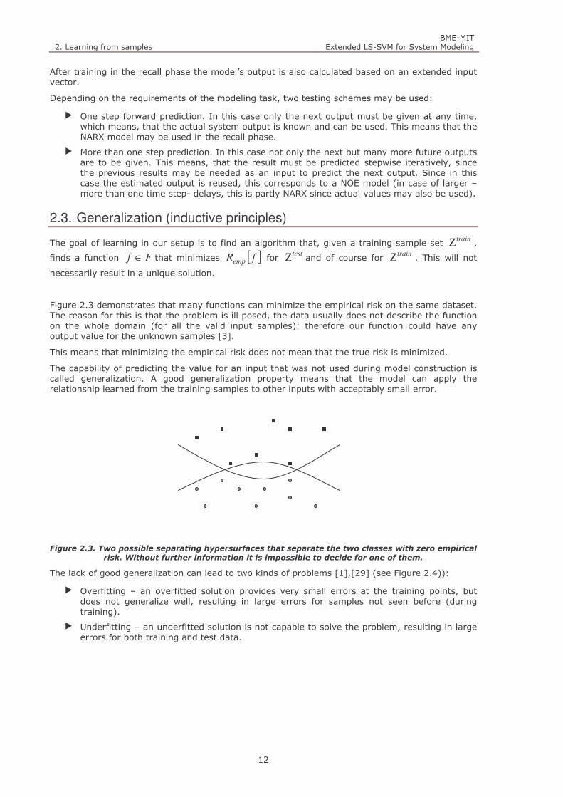
Figure 2.3 demonstrates that many functions can minimize the empirical risk on the same dataset. The reason for this is that the problem is ill posed, the data usually does not describe the function on the whole domain (for all the valid input samples); therefore our function could have any output value for the unknown samples [3].
This means that minimizing the empirical risk does not mean that the true risk is minimized.
The capability of predicting the value for an input that was not used during model construction is called generalization. A good generalization property means that the model can apply the relationship learned from the training samples to other inputs with acceptably small error.
Figure 2.3. Two possible separating hypersurfaces that separate the two classes with zero empirical
risk. Without further information it is impossible to decide for one of them.
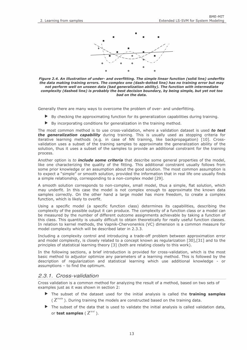
The lack of good generalization can lead to two kinds of problems [1],[29] (see Figure 2.4)):
Overfitting – an overfitted solution provides very small errors at the training points, but does not generalize well, resulting in large errors for samples not seen before (during training).
Underfitting – an underfitted solution is not capable to solve the problem, resulting in large errors for both training and test data.
2. Learning from samples BME-MIT
Extended LS-SVM for System Modeling
13
Figure 2.4. An illustration of under- and overfitting. The simple linear function (solid line) underfits
the data making training errors. The complex one (dash-dotted line) has no training error but may
not perform well on unseen data (bad generalization ability). The function with intermediate
complexity (dashed line) is probably the best decision boundary, by being simple, but yet not too
bad on the data.
Generally there are many ways to overcome the problem of over- and underfitting.
By checking the approximating function for its generalization capabilities during training.
By incorporating conditions for generalization in the training method.
The most common method is to use cross-validation, where a validation dataset is used to test the generalization capability during training. This is usually used as stopping criteria for iterative learning methods (e.g. in case of NN training, like backpropagation) [10]. Cross-validation uses a subset of the training samples to approximate the generalization ability of the solution, thus it uses a subset of the samples to provide an additional constraint for the training process.
Another option is to include some criteria that describe some general properties of the model, like one characterizing the quality of the fitting. This additional constraint usually follows from some prior knowledge or an assumption about the good solution. The most common assumption is to expect a “simple” or smooth solution, provided the information that in real life one usually finds a simple relationship, corresponding to a non-complex model [29].
A smooth solution corresponds to non-complex, small model, thus a simple, flat solution, which may underfit. In this case the model is not complex enough to approximate the known data samples correctly. On the other hand a large model has more freedom, to create a complex function, which is likely to overfit.
Using a specific model (a specific function class) determines its capabilities, describing the complexity of the possible output it can produce. The complexity of a function class or a model can be measured by the number of different outcome assignments achievable by taking a function of this class. This quantity is usually difficult to obtain theoretically for really useful function classes. In relation to kernel methods, the Vapnik-Chervonenkis (VC) dimension is a common measure for model complexity which will be described later in 2.3.3.
Including a complexity control and introducing a trade-off problem between approximation error and model complexity, is closely related to a concept known as regularization [30],[31] and to the principles of statistical learning theory [3] (both are relating closely to this work).
In the following sections, a brief introduction is provided for cross-validation, which is the most basic method to adjustor optimize any parameters of a learning method. This is followed by the description of regularization and statistical learning which use additional knowledge - or assumptions – to find the optimum.
2.3.1. Cross-validation
Cross validation is a common method for analyzing the result of a method, based on two sets of examples just as it was shown in section 2:
The subset of the dataset used for the initial analysis is called the training samples
( trainΖ ). During training the models are constructed based on the training data.
The subset of the data that is used to validate the initial analysis is called validation data,
or test samples ( testΖ ).
2. Learning from samples BME-MIT
Extended LS-SVM for System Modeling
14
The most common types of cross-validation differ on the way they split the available dataset into the two subsets during the iterative process [29]:
Data samples are selected randomly from the initial as test samples, while the remaining ones are retained as the training samples. Usually less than half of the initial sample set is used as validation data.
K-fold cross-validation - In K-fold cross-validation, the original dataset is partitioned into K subsets. In each iteration one of the subsets is retained as the validation data and the remaining K-1 subsets are used as training data. The cross-validation process is then repeated K times (the folds), with each of the K subsets used exactly once as test set. The K errors from the folds then can be averaged (or otherwise combined) to produce an accumulated value.
Leave-one-out cross-validation - As the name suggests, this method uses a single sample from the original dataset as the validation data, and all other as training data. This is repeated such that each sample is used once for testing. This is the same as K-fold cross-validation where K is equal to the number of observations in the original sample.
Based on the results of cross-validation, the performance (quality) of a model can be determined. Using this, an iterative process can be built to optimize parameters of the model, where different parameter settings are tested through cross-validation and the best setup is selected. Often this whole process is referred to as cross-validation.
2.3.2. Regularization
In the previous discussion I demonstrated that generally it is not enough to find a function with minimal empirical risk, since it will most likely overfit the training samples and provide a bad generalization. When expecting to solve a problem by modeling it, one implicitly assumes that the data describe some inherent relationship between the input and the output and it is “simple” enough to be described by the dataset. Thus the output is a “smooth” function of the input. In order to achieve a smooth, simple solution an additional criterion must be included, describing this aspect. This usually concludes in an additional term in the optimization, describing the smoothness (simplicity) of the solution [29].
To produce a good estimation minimizing the true risk on all possible data points (generalization error), a complexity control term is introduced and our solution is obtained by minimizing the following objective function:
[ ] Ω+Ζ CfRemp , (2.13)
This equation shows a regularization approach. A penalty term is added to make the trade-off between the complexity of the function class and the empirical error.
Since this work concerns SVMs, the following section describes the choice inspired by the work of Vapnik. In case of SVMs, the additional term –the regularization controlling the complexity of result- is derived from a more general theory, called statistical learning theory [5].
2.3.3. Statistical learning theory
Statistical learning theory was mainly developed by Vapnik over the last 30 years and it is probably the best available theory for finite sample statistical estimation and predictive learning [29]. This section summarizes the main ideas behind this theory which consists of three parts [3],[5],[32]:
1. The use and consistency of the Empirical Risk Minimization (ERM) principle.
ERM principle gives the very basic grounds for this learning theory, since it connects the (known) empirical risk (see (2.4)) and the (unknown) true risk (see (2.5)). This result is very important since one may only use the samples available, thus only the empirical risk can be accounted for. The result concerning the consistency states that as the number of samples N grows, the empirical estimation becomes more and more accurate.
2. Learning from samples BME-MIT
Extended LS-SVM for System Modeling
15
2. The definition of the VC dimension.
VC dimension is a complexity measure for a function class which can be used to find a model that provides a good solution even in case of a smaller sample set N , thus a good generalization.
3. Structural Risk Minimization.
To utilize these results a method for model construction one must construct a learning method that is able to reduce the VC dimension and the empirical risk at the same time. The structural risk minimization principle provides the backgrounds for controlling the VC dimension (of a model, thus a function class). Finally, in order to construct such models, the SVM (and the other related methods) give constructional, algorithmic solutions for learning problems incorporating these results.
Relying on each other, these principles provide the basic background of statistical learning theory. They are also important from the viewpoint of the propositions of this Thesis, since the propositions of this work reach back to these roots of theory and intend to preserve the advantages of statistical learning.
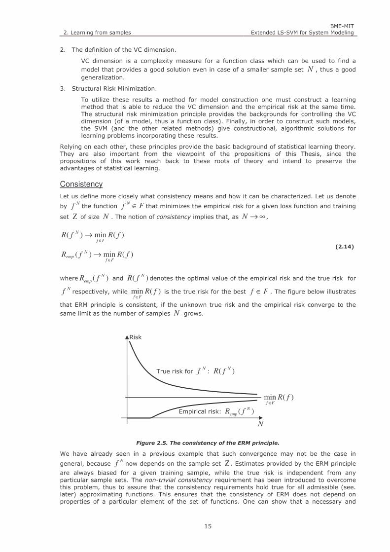
Consistency
Let us define more closely what consistency means and how it can be characterized. Let us denote
by N
f the function FfN ∈ that minimizes the empirical risk for a given loss function and training
set Ζ of size N . The notion of consistency implies that, as ∞→N ,
)(min)( fRfRFf
N
∈→
)(min)( fRfRFf
Nemp
∈→
(2.14)
where )( N
emp fR and )( NfR denotes the optimal value of the empirical risk and the true risk for
Nf respectively, while )(min fR
Ff ∈ is the true risk for the best Ff ∈ . The figure below illustrates
that ERM principle is consistent, if the unknown true risk and the empirical risk converge to the same limit as the number of samples N grows.
Figure 2.5. The consistency of the ERM principle.
We have already seen in a previous example that such convergence may not be the case in
general, because N
f now depends on the sample set Ζ . Estimates provided by the ERM principle
are always biased for a given training sample, while the true risk is independent from any particular sample sets. The non-trivial consistency requirement has been introduced to overcome this problem, thus to assure that the consistency requirements hold true for all admissible (see. later) approximating functions. This ensures that the consistency of ERM does not depend on properties of a particular element of the set of functions. One can show that a necessary and
N
Empirical risk: )( N
emp fR
True risk for N
f : )( NfR
)(min fRFf ∈
Risk

2. Learning from samples BME-MIT
Extended LS-SVM for System Modeling
16
sufficient condition for consistency is the uniform convergence, of the difference between the expected and the empirical risk to zero, over all functions in F . This insight is summarized in the following theorem [3]:
Two-sided uniform convergence in probability, i.e.
0)()(suplim =
>−
∈∞→εfRfRP emp
FfN (2.15)
for all 0>ε , is a necessary and sufficient condition for (non-trivial) consistency of empirical risk
minimization.
More detail on uniform convergence and definition for non-trivial consistency can be found in refs. [3],[4].
It is clear that the rate of this convergence is also important, thus a fast rate of convergence means that even in case of a “smaller” sample set, the empirical risk can be utilized. The rate of convergence can be assured by using a model f from a model class F of proper complexity,
which is characterized by the VC dimension. Knowing that the empirical risk and the true risk for N
f converges to the )(min fRFf ∈
as the number of samples N grow, there is a need to achieve a
fast rate of convergence and at the same time minimize the generalization error for a specific N . These measures are based on the VC dimension:
A finite VC dimension implies a fast rate of convergence.
For a given N the true risk is upper bounded by a formula depending on the VC dimension, thus minimizing it increases the generalization capabilities (minimizes the true error).
Since the condition in the theorem is not only sufficient but also necessary it seems reasonable that any ''good'' learning machine implementing a specific function class should satisfy it. To assure consistency and a fast rate of convergence, a complexity measure, the VC dimension can be utilized.
VC dimension
The VC dimension is a capacity measure for a function set (or a model class), which was originally defined by Vladimir Vapnik and Alexey Chervonenkis [3]-[5]. The notion of this capacity is usually described in the context of classification, because it is more straightforward, but this measure can be used more generally.
Informally, the capacity of a function class -represented by a certain classification model- measures the complexity of the separating surface its functions can make. A function class has a higher capacity, if it can make a versatile separating surface, enabling it to solve more complicated problems. On the other hand, a lower capacity means a simpler surface and therefore a less flexible solution. A good example may be the difference between a high-degree polynomial, and a linear function. It is easy to see that compared to a linear function, a high-degree polynomial can adapt to more complex problems.
To define the capacity of a classifier, first the meaning of shattering is defined: Consider a classification model ),( αZf with some parameter vector α . The model f can shatter a set of
data points ( N
ii 11,1, =−=Ζ x ) if, for each possible labeling of the data points, there exists an α
such that the model ),( αZf evaluates to 1,1− for that set of data points ( f can separate
them).
Probably the simplest example is to consider a linear separating surface as the classification model, which corresponds to the model used by a perceptron. When there are only three points in two dimensions, a line can shatter them, no matter how they are placed or labeled. However, all possible labelings of four points cannot be separated using linear functions.
Usually this is presented as a coloring problem, where the arrangement of the points can be chosen, but then it cannot be changed as the labels on the points are permuted. On the figure below only 2 of the 8 possible permutations are shown for the 3 points, but it is easy to see, that
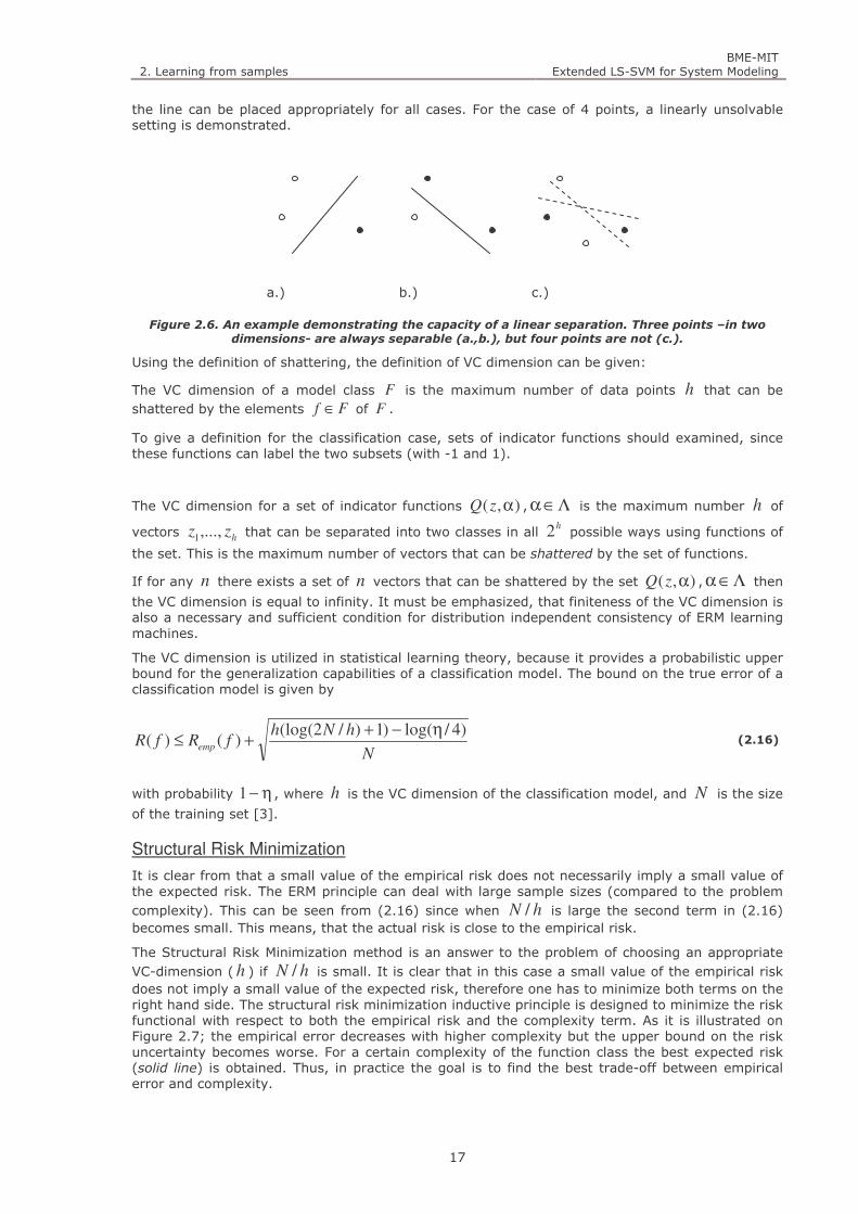
2. Learning from samples BME-MIT
Extended LS-SVM for System Modeling
17
the line can be placed appropriately for all cases. For the case of 4 points, a linearly unsolvable setting is demonstrated.
a.) b.) c.)
Figure 2.6. An example demonstrating the capacity of a linear separation. Three points –in two
dimensions- are always separable (a.,b.), but four points are not (c.).
Using the definition of shattering, the definition of VC dimension can be given:
The VC dimension of a model class F is the maximum number of data points h that can be shattered by the elements Ff ∈ of F .
To give a definition for the classification case, sets of indicator functions should examined, since these functions can label the two subsets (with -1 and 1).
The VC dimension for a set of indicator functions ),( αzQ , Λ∈α is the maximum number h of
vectors hzz ,...,1 that can be separated into two classes in all h2 possible ways using functions of
the set. This is the maximum number of vectors that can be shattered by the set of functions.
If for any n there exists a set of n vectors that can be shattered by the set ),( αzQ , Λ∈α then
the VC dimension is equal to infinity. It must be emphasized, that finiteness of the VC dimension is also a necessary and sufficient condition for distribution independent consistency of ERM learning machines.
The VC dimension is utilized in statistical learning theory, because it provides a probabilistic upper bound for the generalization capabilities of a classification model. The bound on the true error of a classification model is given by
N
hNhfRfR emp
)4/log()1)/2(log()()(
η−++≤ (2.16)
with probability η−1 , where h is the VC dimension of the classification model, and N is the size
of the training set [3].
Structural Risk Minimization
It is clear from that a small value of the empirical risk does not necessarily imply a small value of the expected risk. The ERM principle can deal with large sample sizes (compared to the problem complexity). This can be seen from (2.16) since when hN / is large the second term in (2.16) becomes small. This means, that the actual risk is close to the empirical risk.
The Structural Risk Minimization method is an answer to the problem of choosing an appropriate VC-dimension (h ) if hN / is small. It is clear that in this case a small value of the empirical risk does not imply a small value of the expected risk, therefore one has to minimize both terms on the right hand side. The structural risk minimization inductive principle is designed to minimize the risk functional with respect to both the empirical risk and the complexity term. As it is illustrated on Figure 2.7; the empirical error decreases with higher complexity but the upper bound on the risk uncertainty becomes worse. For a certain complexity of the function class the best expected risk (solid line) is obtained. Thus, in practice the goal is to find the best trade-off between empirical error and complexity.
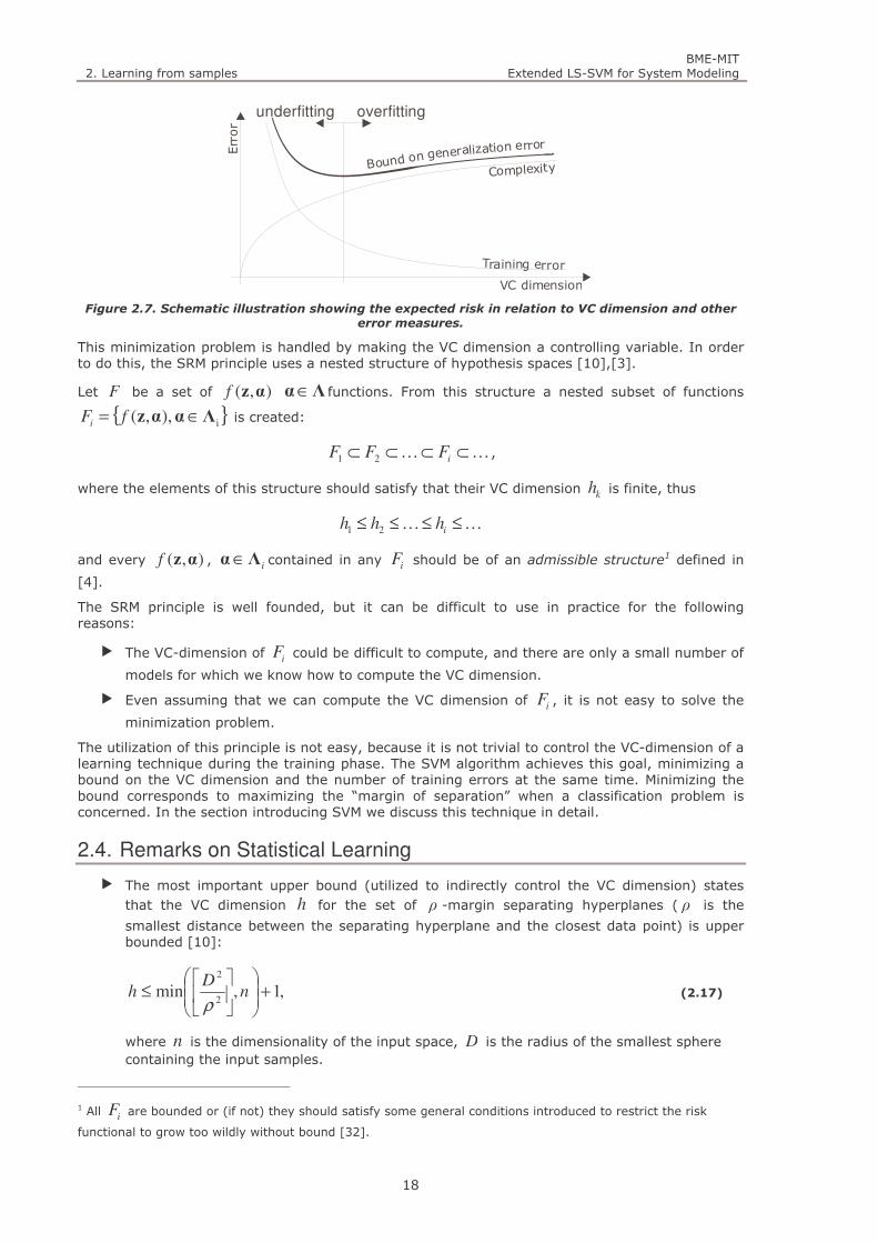
2. Learning from samples BME-MIT
Extended LS-SVM for System Modeling
18
Boen
u n gnd oeralization err
or
Compl tyexi
Training error
Error
VC dimension
underfitting overfitting
Figure 2.7. Schematic illustration showing the expected risk in relation to VC dimension and other
error measures.
This minimization problem is handled by making the VC dimension a controlling variable. In order to do this, the SRM principle uses a nested structure of hypothesis spaces [10],[3].
Let F be a set of ),( αzf Λα∈ functions. From this structure a nested subset of functions
i ),,( Λααz ∈= fFi is created:
KK ⊂⊂⊂⊂ iFFF 21 ,
where the elements of this structure should satisfy that their VC dimension kh is finite, thus
KK ≤≤≤≤ ihhh 21
and every ),( αzf , iΛα∈ contained in any iF should be of an admissible structure1 defined in
[4].
The SRM principle is well founded, but it can be difficult to use in practice for the following reasons:
The VC-dimension of iF could be difficult to compute, and there are only a small number of
models for which we know how to compute the VC dimension.
Even assuming that we can compute the VC dimension of iF , it is not easy to solve the
minimization problem.
The utilization of this principle is not easy, because it is not trivial to control the VC-dimension of a learning technique during the training phase. The SVM algorithm achieves this goal, minimizing a bound on the VC dimension and the number of training errors at the same time. Minimizing the bound corresponds to maximizing the “margin of separation” when a classification problem is concerned. In the section introducing SVM we discuss this technique in detail.
2.4. Remarks on Statistical Learning
The most important upper bound (utilized to indirectly control the VC dimension) states that the VC dimension h for the set of ρ -margin separating hyperplanes ( ρ is the
smallest distance between the separating hyperplane and the closest data point) is upper bounded [10]:
,1,min2
2
+
≤ n
Dh
ρ (2.17)
where n is the dimensionality of the input space, D is the radius of the smallest sphere containing the input samples.
1 All iF are bounded or (if not) they should satisfy some general conditions introduced to restrict the risk
functional to grow too wildly without bound [32].

2. Learning from samples BME-MIT
Extended LS-SVM for System Modeling
19
Based on this bound it can be stated that by maximizing the margin of separation ρ , the
upper bound on the VC dimension is minimized.
The SRM principle does not define a specific function class therefore a structure with a controllable VC dimension must be used [29]. This Thesis involves the following two common structures:
In the first structure, the number of basis functions (m ) is reduced:
∑=
α=m
i
iim gf0
),(),,( vxvαx (2.18)
where ),( ig vx is a basis functions with iv parameters and iα are linear coefficients.
The number of terms m specifies an element of the SRMs nested structure:
),,( vαxkmk fS = , where ...321 mmm << . (2.19)
In this case the goal is to find the optimal number of basis functions for a given dataset in order to achieve the best generalization.
SRM can also be achieved through penalization. Given a set of functions ),( wxf
where w is a parameter vector. Constraining the length of this vector ic<2
w
creates a nested structure on this set of functions:
),,(2
kk cfS <= wwx , where ...321 ccc << . (2.20)
This problem can be solved as a constrained optimization problem where for each
element of the kS structure, the empirical risk and 2
w is minimized
simultaneously.


3. Kernel Methods BME-MIT
Extended LS-SVM for System Modeling
21
3. KERNEL METHODS
In this Thesis a special class of modeling methods is investigated called kernel methods. These methods work, by mapping the data into a higher dimensional kernel space, where the problem can be handled linearly. For the mapping a special nonlinear function, namely a kernel function is used. There are several methods that use this structure but probably the most widely known and used one is the Support Vector Machine. This section introduces the SVM, where the background of kernel methods and functions (e.g. kernel trick) is also detailed (section 3.1). Following this another kernel based method the LS-SVM is also described (section 3.2), which directly provides the backgrounds for the propositions of this thesis. Section 3.3 summarizes the main properties of these methods and sets the goals for the proposed extensions.
3.1. Support Vector Machines
Merging the three ideas of statistical learning a new analytical learning method, the Support Vector Machines [10],[3]-[5],[33]-[39] – proven to be suitable for a wide range of practical applications – were built.
The main goal of this method is to find a hyperplane separating the data with the largest possible margin.
3.1.1. Linearly separable classification (margin maximization)
Let us consider a two-class classification problem (described in section 2.1) and assume that the
patterns - the class represented by the 1+=id desired output and the 1−=id counter class -
are linearly separable. This means, that the decision surface can be defined as
0=+ bT
xw . (3.1)
The adjustable parameters are w and b , the weight vector and the bias, respectively.
From the viewpoint of our training samples, the solution can be rewritten as follows ( 0>a ):
abiT ≥+xw for 1+=id
abiT −≤+xw for 1−=id
(3.2)
By combining these into a single equation and rescaling it with a we get
1)( ≥+ bd iT
i xw for Ni ,...,2,1= , (3.3)
which corresponds to the
i∀ , )sign()( by iT
i += xwx , 1,1 +−∈iy (3.4)
classifier.
Most real life problems are not separable, but these assumptions make it easy to demonstrate the main idea behind SVM. This restriction will be removed later.
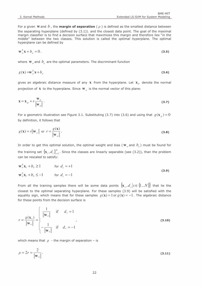
3. Kernel Methods BME-MIT
Extended LS-SVM for System Modeling
22
For a given w and b , the margin of separation ( ρ ) is defined as the smallest distance between
the separating hyperplane (defined by (3.1)). and the closest data point. The goal of the maximal margin classifier is to find a decision surface that maximizes this margin and therefore lies “in the middle” between the two classes. This solution is called the optimal hyperplane. The optimal hyperplane can be defined by
0=+ o
T
o bxw . (3.5)
where ow and ob are the optimal parameters. The discriminant function
o
T
o bg += xwx)( (3.6)
gives an algebraic distance measure of any x from the hyperplane. Let px denote the normal
projection of x to the hyperplane. Since ow is the normal vector of this plane:
o
op r
w
wxx += . (3.7)
For a geometric illustration see Figure 3.1. Substituting (3.7) into (3.6) and using that 0)( =pg x
by definition, it follows that
org wx =)( or o
gr
w
x)(= . (3.8)
In order to get this optimal solution, the optimal weight and bias ( ow and ob ) must be found for
the training set N
iii d1
,=
x . Since the classes are linearly separable (see (3.2)), than the problem
can be rescaled to satisfy:
1≥+ oiTo bxw for 1+=id
1−≤+ oiTo bxw for 1−=id
(3.9)
From all the training samples there will be some data points Nsd ss ...1, ∈x that lie the
closest to the optimal separating hyperplane. For these samples (3.9) will be satisfied with the equality sign, which means that for these samples 1)( =xg or 1)( −=xg . The algebraic distance
for these points from the decision surface is
−=−
=
==
1if1
1if1
)(
s
o
s
o
o
s
d
d
gr
w
w
w
x, (3.10)
which means that ρ - the margin of separation – is
o
rρw
22 == . (3.11)

3. Kernel Methods BME-MIT
Extended LS-SVM for System Modeling
23
Figure 3.1. The geometric interpretation of the distance to the hyperplane in two dimensions.
The training samples lying closest to the separating hyperplane are called support vectors. These samples play a very special role in the described solution, since they are the hardest to classify and also determine the maximal margin between the classes. Most importantly, the support vectors directly determine the position and orientation of the optimal separating hyperplane. As we will see later the solution of a Support Vector Machine is based on these samples.
To summarize the results described in this section, two conclusions are drawn:
The optimal separating hyperplane provides a unique result that maximizes its distance from the classes defined by the training samples.
The margin can be maximized by minimizing the Euclidean norm of the weight vector w .
According to the bound in equation (2.17) the margin maximization minimizes the VC dimension, thus minimizing the norm of the weight vector also means that the VC dimension is minimized. This bound applies for classification problems, but a similar bound exists for regression (if a proper loss function –defined in (3.47)– is used), thus minimizing the weight vector also applies in that case.
This is how the SRM principle is incorporated in the construction of SVM.
Our goal is to find an optimal hyperplane –the optimal value for w and b – that separates the
training samples N
iii
train d1
,=
=Ζ x . This plane minimizes the length of the weight vector
wwwT
F2
1)( = (3.12)
and satisfies the constraints defined by the training samples
1)( ≥+ bd iT
i xw for Ni ,...,2,1= . (3.13)
This constrained optimization problem is called the primal problem. The cost function )(wF is a
convex function of w , while the constraints are linear in w .
This constrained optimization problem can be solved by using Lagrange multipliers:
[ ]∑=
−+−=N
i
i
T
ii
TbdαbJ
1
1)(2
1),,( xwwww αααα (3.14)
where the 0≥iα parameters are the Lagrange multipliers.
This Lagrangian must be minimized with respect to w and b , and maximized with respect to the
iα multipliers:
),,(minmax,
αα
bJb
ww
. (3.15)
1x
2x
optimal hyperplane
x
r
px

3. Kernel Methods BME-MIT
Extended LS-SVM for System Modeling
24
This saddle point is the solution of the problem, which leads to the following conditions:
0w
αw=
∂
∂ ),,( bJ → ∑
=
α=N
i
iii d1
xw (3.16)
0),,(
=∂
∂
b
bJ αw → ∑
=
=αN
i
ii d1
0 (3.17)
Substituting into (3.14) we get:
∑ ∑∑= ==
α+α+α−=N
i
N
i
i
N
i
iii
T
ii
TdbdbJ
1 112
1),,( xwwwαw (3.18)
Using (3.16), the first term is
∑∑∑= ==
αα=α=N
i
N
j
j
T
ijiji
N
i
i
T
ii
Tddd
1 11
xxxwww , (3.19)
while from (3.17) the third term is zero.
The dual problem is to find N
ii 1=α Lagrange multipliers that maximize the objective function
∑∑∑= ==
αα−α=αN
i
N
j
j
T
ijiji
N
i
i ddQ1 11 2
1)( xx (3.20)
with constraints
∑=
=αN
i
ii d1
0
0≥α i for Ni ,...,2,1= .
(3.21)
If the optimal Lagrange multipliers io,α are determined, the optimal weight vector and bias can be
computed by
∑=
α=N
i
iiioo d1
, xw (3.22)
)(1 sT
oob xw−= for 1)( =sd ,where ),( )()( ss dx denotes a support vector. (3.23)
Instead of using the primal formulation (3.4), the SVM classifier can also be constructed in the dual space using the Lagrange multipliers:
+= ∑
=
oTi
N
i
ii bdy xx1
sign α . (3.24)
Again we use the notation, where id means a desired output, while y represents a predicted,
calculated value for a yet “unseen” input x .

3. Kernel Methods BME-MIT
Extended LS-SVM for System Modeling
25
3.1.2. Linearly non-separable classification
So far we have only considered linearly separable patterns, which mean a zero empirical error solution. However for most real life applications this assumption is violated.
An even more important motivation to handle such cases is that in order to get a smooth (simple) solution it is essential to allow some errors. Otherwise the separation surface would become too complex in the input space. By allowing some errors we might get better results and avoid overfitting effects. This means that a trade-off between the empirical risk and the complexity must be found. This will be explained later in the discussion of the nonlinear case.
If the data are not linearly separable then the problem has no feasible solution without error,
therefore slack-variables iξ are introduced to relax the hard-margin constraints:
iiT
i bd ξ−≥+ 1)( xw , 0≥iξ , for Ni ,...,2,1= . (3.25)
For 10 ≤< iξ the data point falls on the right side of the separation hyperplane, but it is inside
the separation margin. If 1>iξ the data sample falls on the wrong side of the separation
hyperplane, which means that it is not classified correctly (see. Figure 3.2).
a.) b.)
Figure 3.2. The use of slack variables to describe the “error” of a sample. a.) The sample falls on
the rights side of the optimal separation surface (dotted line), but it is inside the margin. b.) The
data sample is not classified correctly.
The support vectors are those training samples that exactly meet (3.25) even if 0>iξ , because if
any samples with 0>iξ would be left out, than the decision surface would change. The support
vectors are thus defined exactly the same way as they were in the separable case. In a non-separable case, the solution should not only aim at maximizing the margin, but also at minimizing
∑=
N
i
i
1
ξ . This can be done by finding the correct trade-off between these goals to define one single
optimization problem. SVM solution achieves this by
1. by minimizing the length of w (see section 3.1.1) and
2. by minimizing ∑=
N
i
i
1
ξ (thus an upper bound on the empirical risk).
The criterium function for constructing the optimal separating hyperplane (see. (3.12), (3.13)) is as follows:
1>iξ10 ≤< iξ

3. Kernel Methods BME-MIT
Extended LS-SVM for System Modeling
26
∑=
+=N
i
iT
CF12
1),( ξξ www , (3.26)
with constraints
iiT
i bd ξ−≥+ 1)( xw , 0≥iξ , for Ni ,...,2,1= . (3.27)
From this the following Lagrangian is constructed:
[ ] ∑∑==
−+−+−=N
i
ii
N
i
iiT
ii bdFbJ11
1)(),(),,,,( ξνξαξναξ xwww , 0≥iα , 0≥iν
for Ni ,...,2,1= .
(3.28)
The regularization constant 0>C determines the trade-off between the empirical error and the complexity term. This leads to the dual problem:
∑∑∑= ==
αα−α=αN
i
N
j
j
T
ijiji
N
i
i ddQ1 11 2
1)( xx (3.29)
with constraints
∑=
=αN
i
ii d1
0
Ci ≤α≤0 for Ni ,...,2,1= .
(3.30)
We must note that the only difference, that the slack variables introduced is in the Ci ≤α≤0
constraint, where the Lagrange multipliers are now upper bounded by C . Except for this
modification everything else (e.g. the computation of ow and ob ) is exactly the same as earlier.
This can be seen, by exploiting the fact that for all support vectors, the slack variable iξ is zero.
In the above described linearly non-separable case a hyper plane is used, but misclassifications are allowed. To further enhance the solution for these problems a nonlinear separation surface may be used, which allows a more flexible solution. In order to achieve such a solution, an indirect approach is used. The training samples are nonlinearly mapped to a new –usually higher dimensional- space, where a linear solution is constructed. This linear separation surface corresponds to a nonlinear surface in the primal space. Instead of mapping this back to the original space and using the nonlinear separation; the calculations are done in the space, where the problem is linear. In nonlinear SVM solutions a special “two step” nonlinear mapping is used based on the kernel trick described in the sequel.
3.1.3. Kernel trick
Using a nonlinear mapping is the key concept in handling nonlinear problems linearly. In order to gain a linear problem, first the training data is mapped into a high dimensional feature space
which can possibly be infinite dimensional. Luckily, the explicit construction of the ( )xϕ mapping,
or the resulting feature space is not needed in support vector methods.
For any symmetric, continuous function ( )yx,K that satisfies the Mercer’s condition [4], there
exists a Hilbert space H , and a mapping Hp →ℜ:ϕ , and 0>λ i numbers
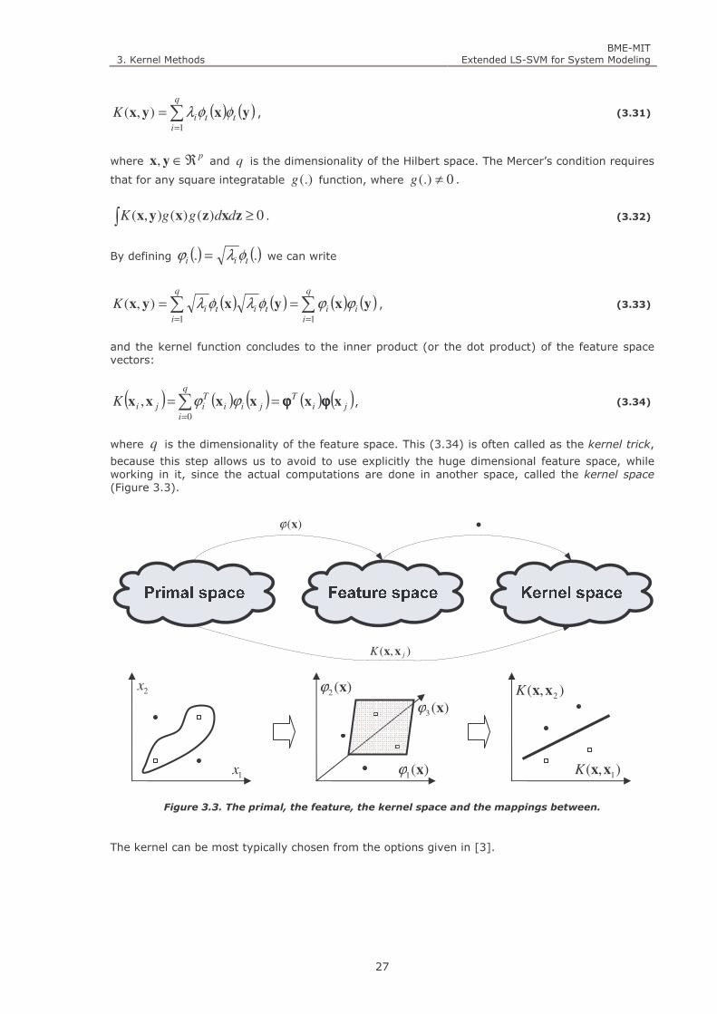
3. Kernel Methods BME-MIT
Extended LS-SVM for System Modeling
27
( ) ( )yxyx ιι φφλ∑=
=q
iiK
1
),( , (3.31)
where pℜ∈yx, and q is the dimensionality of the Hilbert space. The Mercer’s condition requires
that for any square integratable (.)g function, where 0(.) ≠g .
0)()(),( ≥∫ zxzxyx ddggK . (3.32)
By defining ( ) ( ).. ιφλϕ ii = we can write
( ) ( ) ( ) ( )∑∑==
==q
iiii
q
iiK
11
),( yxyxyx ϕϕφλφλ ιι , (3.33)
and the kernel function concludes to the inner product (or the dot product) of the feature space vectors:
( ) ( ) ( ) ( ) ( )jiT
q
ijii
TijiK xxxxxx ϕϕϕϕϕϕϕϕ==∑
=0
, ϕϕ , (3.34)
where q is the dimensionality of the feature space. This (3.34) is often called as the kernel trick,
because this step allows us to avoid to use explicitly the huge dimensional feature space, while working in it, since the actual computations are done in another space, called the kernel space (Figure 3.3).
)(xϕ
),( jK xx
•
Figure 3.3. The primal, the feature, the kernel space and the mappings between.
The kernel can be most typically chosen from the options given in [3].
1x
2x
)(1 xϕ
)(2 xϕ
),( 1xxK
),( 2xxK
)(3 xϕ

3. Kernel Methods BME-MIT
Extended LS-SVM for System Modeling
28
Table 3.1. The most common kernel functions.
LINEAR SVM ( ) xxxx TiiK =,
POLYNOMIAL SVM OF
DEGREE d ( ) ( )dT
iiK 1, += xxxx
GAUSSIAN SVM ( ) 22exp, σiiK xxxx −−= , where σ is a constant.
MLP SVM ( ) )tanh(, θ+= xxxx Tii kK , k and θ are properly chosen constants, since
not all combinations may be used.
From the kernel function values usually a matrix is built, called the kernel matrix, which contains all combinations of the N training samples.
=
),(),(),(
),(),(),(
),(),(),(
1
1
1111
NNNiN
iNiii
Ni
KKK
KKK
KKK
xxxxxx
xxxxxx
xxxxxx
Ω
LL
MOMOM
LL
MOMOM
LL
, (3.35)
An important property of this matrix is that it is an NN × symmetric matrix.
3.1.4. Nonlinear Support Vector classifier
The extension from the linear case to the nonlinear one is pretty straightforward. The data samples are mapped to a higher dimensional feature space - where they are linearly separable –
and separated linearly. This is simply done by replacing ix with )( ixϕ and proceed as described
in section 3.1.2.. Thus a maximal margin linear separation is done in the feature space. The feature space dimensionality must be as high as needed to achieve such separation. In case of RBF networks this dimensionality is predefined, but in case of SVM the feature space – as the kernel trick is applied – is not used directly, thus the dimensionality of this space is “automatically”
(implicitly) derived. It is important to mention, that )( ixϕ and consequently w can be arbitrary
high (even infinite) dimensional. This is especially important, because it makes it impossible to solve the primal problem for w , which could be done in the linear SVM. In this case the problem is solved for its finite dimensional dual result α .
The nonlinear SVM can be derived as follows. The linear separation surface in the feature space can be defined according to the mapped points.
iiT
i bd ξ−≥+ 1))(( xw ϕϕϕϕ , 0≥iξ , for Ni ,...,2,1= . (3.36)
The qp ℜ→ℜ:(.)ϕϕϕϕ mapping is not defined explicitly at this point, because later we will change to
a kernel function, by applying the kernel trick. The criterion function becomes:
∑=
+=N
i
iT
CF12
1),( ξξ www , (3.37)
with constraints
iiT
i bd ξ−≥+ 1))(( xw ϕϕϕϕ , 0≥iξ , for Ni ,...,2,1= . (3.38)

3. Kernel Methods BME-MIT
Extended LS-SVM for System Modeling
29
The constructed Lagrangian is
[ ] ∑∑==
−+−+−=N
i
ii
N
i
iiT
ii bdFbJ11
1))((),(),,,,( ξνξαξναξ xwww ϕϕϕϕ , (3.39)
with Lagrange multipliers 0≥iα , 0≥iν for Ni ,...,2,1= . The saddle point is calculated as
),,,,(minmax,,,
ναξξνα
bJb
ww
. (3.40)
The partial derivates:
0w
w=
∂
ναξ∂ ),,,,( bJ → ∑
=
=N
i
iiid1
)(xw ϕϕϕϕα (3.41)
0),,,,(
=∂
ναξ∂
b
bJ w → ∑
=
=N
i
iid1
0α (3.42)
0),,,,(
=∂
∂
i
bJ
ξ
ναξw → Ci ≤≤ α0 , Ni ,...,2,1= (3.43)
Using the kernel trick (3.1.3) ( ) ( ) ( )ji
T
jiK xxxx ϕϕϕϕϕϕϕϕ=, , this leads to the dual problem:
∑∑∑= ==
αα−α=αN
i
N
j
j
T
ijiji
N
i
i KddQ1 11
)(2
1)( xx (3.44)
with constraints
∑=
=αN
i
ii d1
0 , Ci ≤α≤0 for Ni ,...,2,1= . (3.45)
Finally the nonlinear SVM classifier is formulated
( )
+= ∑
=
bKdy i
N
i
ii xx,sign1
α (3.46)
3.1.5. Support Vector Regression
In this section the Support Vector Regression (SVR) formulation is presented. The general background of this method is similar to the classification case therefore the final nonlinear SVR formulation is presented in the sequel.
A training data set is as described in section 2.1. The N
iii d 1, =x sample set is obtained, where
pi R∈x represents a p-dimensional input vector and Rd i ∈ is the scalar target output.
A loss function is also defined, representing the cost of the deviation from the target output id for
each ix input. In most cases it is the ε –insensitive loss function ( εL ), but one can use other
(e.g. non–linear) loss functions, such as given in [37].
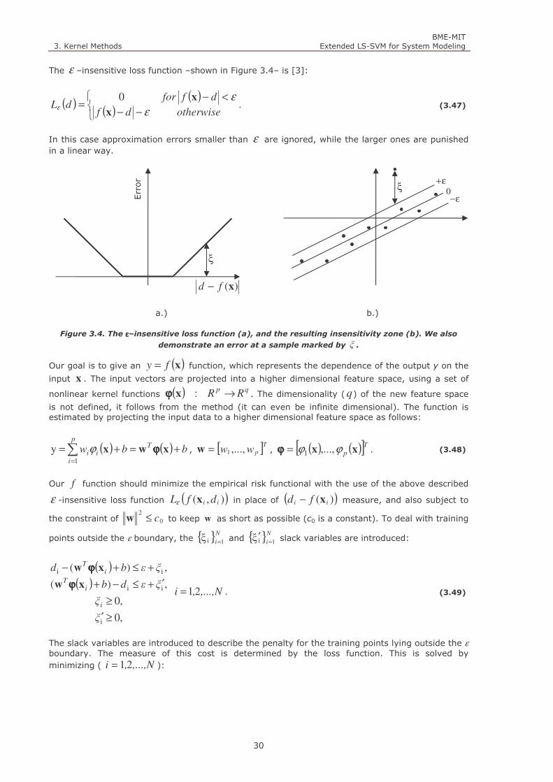
3. Kernel Methods BME-MIT
Extended LS-SVM for System Modeling
30
The ε –insensitive loss function –shown in Figure 3.4– is [3]:
( )( )
( )
−−
<−=
otherwisedf
dffordL
ε
εε
x
x 0. (3.47)
In this case approximation errors smaller than ε are ignored, while the larger ones are punished in a linear way.
a.) b.)
Figure 3.4. The εεεε–insensitive loss function (a), and the resulting insensitivity zone (b). We also
demonstrate an error at a sample marked by ξ .
Our goal is to give an ( )xfy = function, which represents the dependence of the output y on the
input x . The input vectors are projected into a higher dimensional feature space, using a set of
nonlinear kernel functions ( ) qpRR →:xϕϕϕϕ . The dimensionality (q) of the new feature space
is not defined, it follows from the method (it can even be infinite dimensional). The function is estimated by projecting the input data to a higher dimensional feature space as follows:
( ) ( ) bbw Ti
p
ii +=+=∑
=
xwx ϕϕϕϕϕ1
y , [ ]T
pww ,...,1=w , ( ) ( )[ ]Tp xx ϕϕ ,...,1=ϕϕϕϕ . (3.48)
Our f function should minimize the empirical risk functional with the use of the above described
ε -insensitive loss function ( )),( ii dfL xε in place of ( ))( ii fd x− measure, and also subject to
the constraint of 0
2c≤w to keep w as short as possible (c0 is a constant). To deal with training
points outside the ε boundary, the N
i 1iξ = and N
i 1iξ =′ slack variables are introduced:
( )( )
,...,N,i
ξ
ξ
ξεdb
ξεbd
i
iT
iT
21
,0
,0
,)(
,)(
i
ii
ii
=
≥′
≥
′+≤−+
+≤+−
xw
xw
ϕϕϕϕ
ϕϕϕϕ
. (3.49)
The slack variables are introduced to describe the penalty for the training points lying outside the ε boundary. The measure of this cost is determined by the loss function. This is solved by minimizing ( ,...,N,i 21 = ):
0
ε+
ε−
ξ
)(xfd −
ξ
Error

3. Kernel Methods BME-MIT
Extended LS-SVM for System Modeling
31
( ) ( )
′++=′ ∑
=
N
i
TCF
1
ii ξξ2
1ξξ,, www ,
( )( )
.0ξ,ξ)(
,0ξ ,ξ)(
iii
iii
≥+≤−+
≥′′+≤+−
εdb
εbd
iT
iT
xw
xw
ϕϕϕϕ
ϕϕϕϕ (3.50)
The first term stands for the minimization of w , while the C constant is the trade–off parameter between this and the minimization of training data errors. This constrained optimization can be defined as a Lagrangian function, which can be solved by Quadratic Programming (QP) in its dual form.
Primal problem:
( ) ( ) [ ]
[ ] ( )∑∑
∑∑
==
==
′′+−′++−−′−
++−+−+′+=′′′
N
iii
N
iii
Ti
N
iii
Ti
TN
iii
bd
dbCJ
1ii
1i
1i
1
)(
)(2
1,,,,ξξ,,
ξγξγξεα
ξεαξξγγαα
xw
xwwww
ϕϕϕϕ
ϕϕϕϕ
(3.51)
The primal problem deals with convex cost function and linear constraint; therefore from this constrained optimization problem a dual problem can be constructed. To do this the Karush–Kuhn–Tucker (KKT) conditions [4] are used.
Dual problem:
( ) ( ) ( )
( )( ) ( )ji
N
i
N
j
N
i
i
N
i
i
K
dQ
xx ,2
1
,
1 1
jjii
1
ii
1
ii
∑∑
∑∑
= =
==
′−′−−
′+−′+=′
αααα
αααεαααα
(3.52)
with constraints:
( ) NiCCN
i
,....,2,1 ,0 ,0 ,0 ii
1
ii =≤′≤≤≤=′+∑=
αααα (3.53)
Finally our function f is calculated from equation (3.54), where iα and iα′ are the Lagrange
multipliers and based upon the Mercer condition ( ) ( ) ( )jiT
jiK xxxx ϕϕ=, is the inner–product
kernel function.
( ) ( ) bKy i
N
i
ii +′−=∑=
xx,1
αα (3.54)
The nonzero multipliers ( ( ) 0≠′− ii αα ) mark their corresponding input data points as support
vectors. The bias b follows from the KKT conditions [10],[3]-[5].
The user defined parameters C and ε control the smoothness of the resulting function. We must also choose the parameters of the kernel function. In our Gaussian kernel based structure it means the selection of a suitable σ or a σσσσ vector. In practice, it’s very hard to determine the optimal values for these three parameters, because no universal approach is available. This Thesis does not discuss these problems, but some results can be found in refs. [40]-[45].
3.1.6. Fast SVM solutions
The main problem with this method is its high algorithmic complexity (caused by the Quadratic Programming involved), namely its slow construction and extensive memory requirements. To overcome these problems, several modifications and extensions of the method has been proposed. These solutions can be categorized into two major solution schemes:

3. Kernel Methods BME-MIT
Extended LS-SVM for System Modeling
32
Ones that solve the original SVM problem more effectively. These methods are developed to give a more efficient solution for the QP problem.
Ones that “slightly” change the original SVM formulation to achieve a simpler problem that can be solved more effectively.
Although the solutions presented in this Thesis are somewhat related to providing a more effective support vector based model, the primary goal –namely to get a robust, sparse LS-SVM- is different. Therefore only a brief overview is presented for these methods. As it will be shown, some ideas presented will be used later in the constriction of the extended LS-SVM.
Efficient QP solvers
These algorithms are mostly iterative methods that decompose the large problem into smaller optimization tasks [46]–[57]. These methods are commonly known as “chunking” algorithms, where the methods mainly differ in the way they determine the decomposed sub–problems. The traditional “chunking” [46] may not reduce the problem enough, therefore different modifications are available.
The chunking algorithm starts from a randomly selected subset (called working set) of the data, which is modified iteratively, until all samples meet the KKT optimality conditions:
1)(
1)(0
1)(0
≤⇒==⇒<<≥⇒=
iii
iii
iii
fdC
fdC
fd
x
x
x
αα
α (3.55)
The main problem with the original chunking method is that the size of the solvable QP problem depends from the number of SVs. To overcome this problem, the working set size is limited. The main chunking techniques are Osuna’s algorithm and Sequential Minimal Optimization (SMO) [51]. Osuna et all. suggest maximizing the reduced QP sub–problems of a fixed size. To achieve the greatest reduction, a special case of SMO brakes up the large quadratic problem into a series of smallest possible QP problems, consisting working sets of size 2 is used. This set can be solved analytically [47],[48], since it consists of only two Lagrange multipliers, which are jointly optimized at every iteration. Successive overrelaxation (SOR) has also been applied to large SVM problems [49].
Figure 3.5. The different chunking strategies. The thin line represents the sample set, while the
thick line shows, the actual working set. Three iterations are illustrated.
Reformulating the optimization problem
The two methods described in the sequel are the works of Mangasarian who created the Generalized Support Vector Machine (GSVM) [58], which generalizes the optimization problem of SVM. Based on this a smoothing method is applied to the traditional SVM to achieve a fast reformulation called Smooth Support Vector Machines (SSVM) [59]. This smooth SVM is further extended with a special reduction method that concludes to a much smaller optimization problem providing an even faster calculation. This modeling approach is called Reduced Support Vector Machine (RSVM) [60]. Changing the optimization problem, the QP can be changed to more effective optimizations, such as linear programming, or simple gradient methods. The reduction of RSVM speeds the calculations even more, by reducing the size of the optimization problem.
Chunking
Osuna
SMO
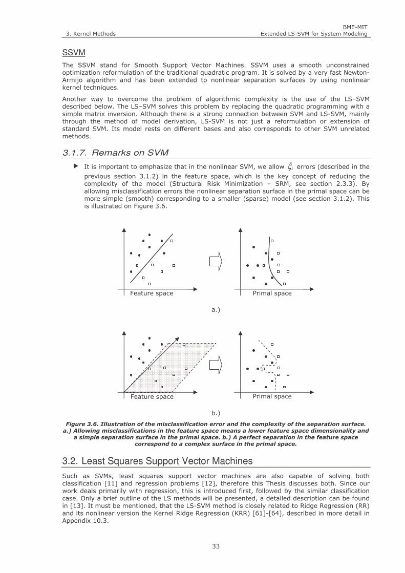
3. Kernel Methods BME-MIT
Extended LS-SVM for System Modeling
33
SSVM
The SSVM stand for Smooth Support Vector Machines. SSVM uses a smooth unconstrained optimization reformulation of the traditional quadratic program. It is solved by a very fast Newton-Armijo algorithm and has been extended to nonlinear separation surfaces by using nonlinear kernel techniques.
Another way to overcome the problem of algorithmic complexity is the use of the LS–SVM described below. The LS–SVM solves this problem by replacing the quadratic programming with a simple matrix inversion. Although there is a strong connection between SVM and LS-SVM, mainly through the method of model derivation, LS-SVM is not just a reformulation or extension of standard SVM. Its model rests on different bases and also corresponds to other SVM unrelated methods.
3.1.7. Remarks on SVM
It is important to emphasize that in the nonlinear SVM, we allow iξ errors (described in the
previous section 3.1.2) in the feature space, which is the key concept of reducing the complexity of the model (Structural Risk Minimization – SRM, see section 2.3.3). By allowing misclassification errors the nonlinear separation surface in the primal space can be more simple (smooth) corresponding to a smaller (sparse) model (see section 3.1.2). This is illustrated on Figure 3.6.
a.)
b.)
Figure 3.6. Illustration of the misclassification error and the complexity of the separation surface.
a.) Allowing misclassifications in the feature space means a lower feature space dimensionality and
a simple separation surface in the primal space. b.) A perfect separation in the feature space
correspond to a complex surface in the primal space.
3.2. Least Squares Support Vector Machines
Such as SVMs, least squares support vector machines are also capable of solving both classification [11] and regression problems [12], therefore this Thesis discusses both. Since our work deals primarily with regression, this is introduced first, followed by the similar classification case. Only a brief outline of the LS methods will be presented, a detailed description can be found in [13]. It must be mentioned, that the LS-SVM method is closely related to Ridge Regression (RR) and its nonlinear version the Kernel Ridge Regression (KRR) [61]-[64], described in more detail in Appendix 10.3.
Feature space Primal space
Feature space Primal space

3. Kernel Methods BME-MIT
Extended LS-SVM for System Modeling
34
3.2.1. LS-SVM regression
Our regression problem is the same as earlier, defined in section 2.1. Let’s define the solution in the following form:
bbwy Ti
q
i
i +=+=∑=
)()()(1
xwxx ϕϕϕϕϕ ,
Tqwww ],...,,[ 21=w , T
q ],...,,[ 21 ϕϕϕ=ϕϕϕϕ .
(3.56)
The q
ii 1)( =xϕ is a set of given linearly independent basis functions, which maps the input data
into an q –dimensional feature space. The dimension of the feature space may be very large, even
infinite.
The main difference from the standard SVM is in the constraints. LS-SVM applies equality constraints, so the constrained optimization task will be:
∑=
+=N
i
iT
beCJ
1
2
,, 2
1
2
1),(min wwew
ew (3.57)
with constraints:
( ) iiT
i ebd ++= xw ϕϕϕϕ , Ni ,...,1= . (3.58)
The first term is responsible for finding a smooth solution, while the second one minimizes the training errors (C is the trade–off parameter between the terms). From this, the following Lagrangian can be formed:
( ) ∑=
−++−=N
i
iiiT
i debJbL1
),();,,( xwewαew ϕϕϕϕα (3.59)
where the iα parameters are the Lagrange multipliers. The conditions for optimality are the followings:
( ) NidebL
NieCe
Lb
L
L
iiiT
i
ii
i
N
i
i
N
i
ii
,...,100
,...,1 0
00
)(
1
1
==−++→=∂
∂
==→=∂
∂
=→=∂
∂
=→=∂
∂
∑
∑
=
=
xw
xw0w
ϕϕϕϕ
ϕϕϕϕ
α
α
α
α
(3.60)
The corresponding linear equation set (a linear Karush–Kuhn–Tucker system [13]) is:
=
+ − dαIΩ1
1 001
b
C
T
r
r
, T
Nddd ],...,,[ 21=d , T
N ],..,,[ 21 ααα=α , T]1,...,1[=1r
,
( ) ( )ji
T
jiji K xxxx ϕϕϕϕϕϕϕϕ==Ω ),(, .
(3.61)
3. Kernel Methods BME-MIT
Extended LS-SVM for System Modeling
35
where ),( jiK xx is a kernel function, +ℜ∈C is a positive constant, b is the bias and the
response of the LS-SVM can be obtained in the form:
( )∑ =+=
N
iii bKαy
1,)( xxx . (3.62)
It must also be mentioned that LS-SVM regression is closely related to Gaussian processes and regularization networks in that the obtained linear systems are equivalent [11].
3.2.2. LS-SVM classification
The main idea is exactly the same as shown above. Given the N
iii ,d 1=x training data set, where
pi ℜ∈x represents a p –dimensional input vector with 1,1 +−∈id labels, a classifier of form
[ ]bbwyT
i
q
ii +=
+= ∑
=
)(sign)(sign)(1
xwxx ϕϕϕϕϕ ,
Tqwww ],...,,[ 21=w , T
q ],...,,[ 21 ϕϕϕ=ϕϕϕϕ .
(3.63)
is constructed. The optimization problem is ( Ni ,...,1= ):
∑=
+=N
i
iT
pb
eCJ1
2
,, 2
1
2
1),(min wwew
ew, with constraints: ( )[ ] ii
Ti ebd −=+ 1xw ϕϕϕϕ . (3.64)
The Lagrangian is the following:
( )[ ] ∑=
+−+−=N
i
iiT
ii ebdJbL1
1),();,,( xwewαew ϕϕϕϕα (3.65)
where iα are the Lagrange multipliers.
The conditions for optimality –similarly to the regression case– can be given by the partial derivatives:
( )[ ] NiebdL
NieCe
L
db
L
dL
iiT
i
i
ii
i
N
i
ii
N
i
iii
,...,1010
,...,1 0
00
)(
1
1
==+−+→=∂
∂
==→=∂
∂
=→=∂
∂
=→=∂
∂
∑
∑
=
=
xw
xw0w
ϕϕϕϕ
ϕϕϕϕ
α
α
α
α
. (3.66)
So the linear equation set of the classification case is:
=
+ − 1αIΩdd r00
1b
C
T
, T
Nddd ],...,,[ 21=d , T
N ],..,,[ 21 ααα=α , T]1,...,1[=1r
,
),(, jijiji Kdd xx=Ω .
(3.67)
where +ℜ∈C is again a positive constant, b is the bias.
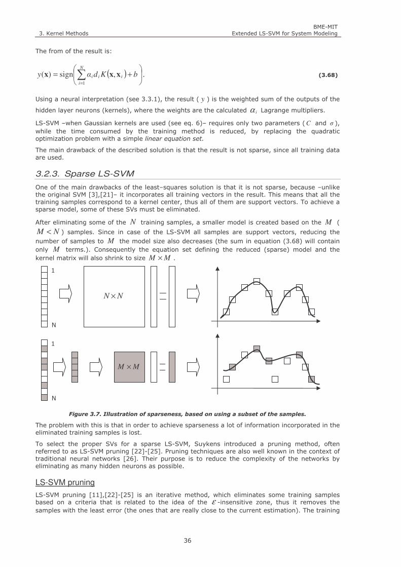
3. Kernel Methods BME-MIT
Extended LS-SVM for System Modeling
36
The from of the result is:
( )
+= ∑
=
N
i
iii bKdαy1
,sign)( xxx . (3.68)
Using a neural interpretation (see 3.3.1), the result ( y ) is the weighted sum of the outputs of the
hidden layer neurons (kernels), where the weights are the calculated iα Lagrange multipliers.
LS-SVM –when Gaussian kernels are used (see eq. 6)– requires only two parameters (C and σ ), while the time consumed by the training method is reduced, by replacing the quadratic optimization problem with a simple linear equation set.
The main drawback of the described solution is that the result is not sparse, since all training data are used.
3.2.3. Sparse LS-SVM
One of the main drawbacks of the least–squares solution is that it is not sparse, because –unlike the original SVM [3],[21]– it incorporates all training vectors in the result. This means that all the training samples correspond to a kernel center, thus all of them are support vectors. To achieve a sparse model, some of these SVs must be eliminated.
After eliminating some of the N training samples, a smaller model is created based on the M (
NM < ) samples. Since in case of the LS-SVM all samples are support vectors, reducing the number of samples to M the model size also decreases (the sum in equation (3.68) will contain only M terms.). Consequently the equation set defining the reduced (sparse) model and the kernel matrix will also shrink to size MM × .
Figure 3.7. Illustration of sparseness, based on using a subset of the samples.
The problem with this is that in order to achieve sparseness a lot of information incorporated in the eliminated training samples is lost.
To select the proper SVs for a sparse LS-SVM, Suykens introduced a pruning method, often referred to as LS-SVM pruning [22]-[25]. Pruning techniques are also well known in the context of traditional neural networks [26]. Their purpose is to reduce the complexity of the networks by eliminating as many hidden neurons as possible.
LS-SVM pruning
LS-SVM pruning [11],[22]-[25] is an iterative method, which eliminates some training samples based on a criteria that is related to the idea of the ε -insensitive zone, thus it removes the samples with the least error (the ones that are really close to the current estimation). The training
1
N
1
N
NN ×
MM ×
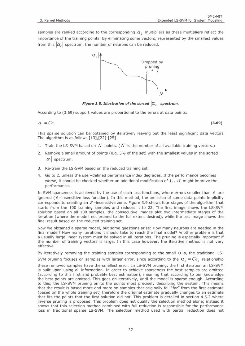
3. Kernel Methods BME-MIT
Extended LS-SVM for System Modeling
37
samples are ranked according to the corresponding kα multipliers as these multipliers reflect the
importance of the training points. By eliminating some vectors, represented by the smallest values
from this kα spectrum, the number of neurons can be reduced.
Figure 3.8. Illustration of the sorted kα spectrum.
According to (3.69) support values are proportional to the errors at data points:
ii Ce=α . (3.69)
This sparse solution can be obtained by iteratively leaving out the least significant data vectors The algorithm is as follows [13],[22]-[25]
1. Train the LS-SVM based on N points. ( N is the number of all available training vectors.)
2. Remove a small amount of points (e.g. 5% of the set) with the smallest values in the sorted
iα spectrum.
3. Re-train the LS-SVM based on the reduced training set.
4. Go to 2, unless the user–defined performance index degrades. If the performance becomes worse, it should be checked whether an additional modification of C , σ might improve the performance.
In SVM sparseness is achieved by the use of such loss functions, where errors smaller than ε are ignored (ε –insensitive loss function). In this method, the omission of some data points implicitly corresponds to creating an ε –insensitive zone. Figure 3.9 shows four stages of the algorithm that starts from the 100 training samples and reduces it to 22. The first image shows the LS-SVM solution based on all 100 samples, the consecutive images plot two intermediate stages of the iteration (where the modell not pruned to the full extent desired), while the last image shows the final result based on the reduced training set.
Now we obtained a sparse model, but some questions arise: How many neurons are needed in the final model? How many iterations it should take to reach the final model? Another problem is that a usually large linear system must be solved in all iterations. The pruning is especially important if the number of training vectors is large. In this case however, the iterative method is not very effective.
By iteratively removing the training samples corresponding to the small α -s, the traditional LS-
SVM pruning focuses on samples with larger error, since according to the kk Ce=α relationship
these removed samples have the smallest error. In LS-SVM pruning, the first iteration an LS-SVM is built upon using all information. In order to achieve sparseness the best samples are omitted (according to this first and probably best estimation), meaning that according to our knowledge the best points are omitted. This goes on iteratively, until the model is sparse enough. According to this, the LS-SVM pruning omits the points most precisely describing the system. This means that the result is based more and more on samples that originally fall “far” from the first estimate (based on the whole training set) therefore the original estimate gradually changes to an estimate that fits the points that the first solution did not. This problem is detailed in section 4.5.2 where inverse pruning is proposed. This problem does not qualify the selection method alone; instead it shows that this selection method combined with full reduction is responsible for the performance loss in traditional sparse LS-SVM. The selection method used with partial reduction does not
kα
N
Dropped by pruning
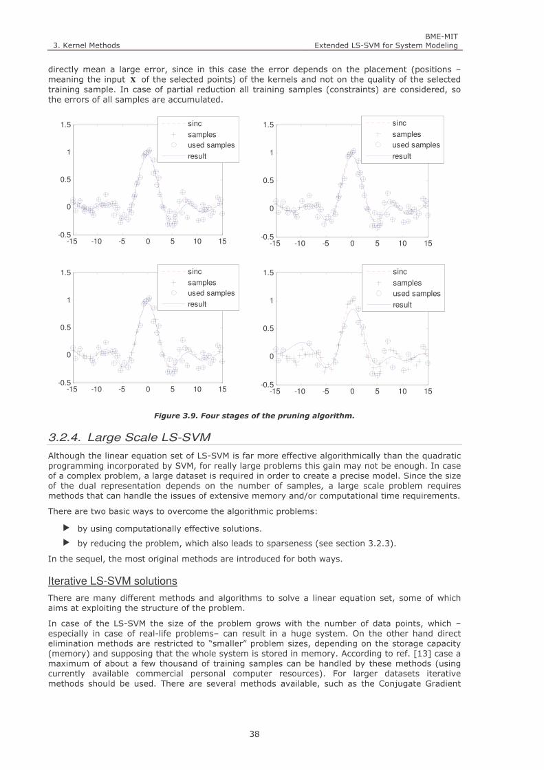
3. Kernel Methods BME-MIT
Extended LS-SVM for System Modeling
38
directly mean a large error, since in this case the error depends on the placement (positions – meaning the input x of the selected points) of the kernels and not on the quality of the selected training sample. In case of partial reduction all training samples (constraints) are considered, so the errors of all samples are accumulated.
Figure 3.9. Four stages of the pruning algorithm.
3.2.4. Large Scale LS-SVM
Although the linear equation set of LS-SVM is far more effective algorithmically than the quadratic programming incorporated by SVM, for really large problems this gain may not be enough. In case of a complex problem, a large dataset is required in order to create a precise model. Since the size of the dual representation depends on the number of samples, a large scale problem requires methods that can handle the issues of extensive memory and/or computational time requirements.
There are two basic ways to overcome the algorithmic problems:
by using computationally effective solutions.
by reducing the problem, which also leads to sparseness (see section 3.2.3).
In the sequel, the most original methods are introduced for both ways.
Iterative LS-SVM solutions
There are many different methods and algorithms to solve a linear equation set, some of which aims at exploiting the structure of the problem.
In case of the LS-SVM the size of the problem grows with the number of data points, which –especially in case of real-life problems– can result in a huge system. On the other hand direct elimination methods are restricted to “smaller” problem sizes, depending on the storage capacity (memory) and supposing that the whole system is stored in memory. According to ref. [13] case a maximum of about a few thousand of training samples can be handled by these methods (using currently available commercial personal computer resources). For larger datasets iterative methods should be used. There are several methods available, such as the Conjugate Gradient
-15 -10 -5 0 5 10 15-0.5
0
0.5
1
1.5
sinc
samples
used samples
result
-15 -10 -5 0 5 10 15-0.5
0
0.5
1
1.5
sinc
samples
used samples
result
-15 -10 -5 0 5 10 15-0.5
0
0.5
1
1.5
sinc
samples
used samples
result
-15 -10 -5 0 5 10 15-0.5
0
0.5
1
1.5
sinc
samples
used samples
result
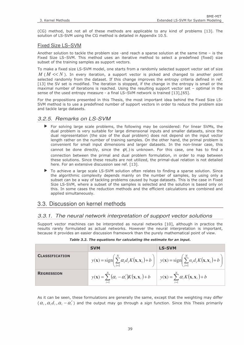
3. Kernel Methods BME-MIT
Extended LS-SVM for System Modeling
39
(CG) method, but not all of these methods are applicable to any kind of problems [13]. The solution of LS-SVM using the CG method is detailed in Appendix 10.5.
Fixed Size LS–SVM
Another solution to tackle the problem size -and reach a sparse solution at the same time – is the Fixed Size LS–SVM. This method uses an iterative method to select a predefined (fixed) size subset of the training samples as support vectors.
To make a fixed size LS-SVM model, one starts from a randomly selected support vector set of size M ( NM << ). In every iteration, a support vector is picked and changed to another point selected randomly from the dataset. If this change improves the entropy criteria defined in ref. [13] the SV set is modified. The iteration is stopped, if the change in the entropy is small or the maximal number of iterations is reached. Using the resulting support vector set – optimal in the sense of the used entropy measure - a final LS–SVM network is trained [13],[65].
For the propositions presented in this Thesis, the most important idea behind the Fixed Size LS-SVM method is to use a predefined number of support vectors in order to reduce the problem size and tackle large datasets.
3.2.5. Remarks on LS-SVM
For solving large scale problems, the following may be considered: For linear SVMs, the dual problem is very suitable for large dimensional inputs and smaller datasets, since the dual representation (the size of the dual problem) does not depend on the input vector length rather on the number of training samples. On the other hand, the primal problem is convenient for small input dimensions and larger datasets. In the non-linear case, this cannot be done directly, since the (.)ϕ is unknown. For this case, one has to find a
connection between the primal and dual problem formulation, in order to map between these solutions. Since these results are not utilized, the primal-dual relation is not detailed here. For an extensive discussion see ref. [13].
To achieve a large scale LS-SVM solution often relates to finding a sparse solution. Since the algorithmic complexity depends mainly on the number of samples, by using only a subset can be a way of tackling problems caused by huge datasets. This is the case in Fixed Size LS-SVM, where a subset of the samples is selected and the solution is based only on this. In some cases the reduction methods and the efficient calculations are combined and applied simultaneously.
3.3. Discussion on kernel methods
3.3.1. The neural network interpretation of support vector solutions
Support vector machines can be interpreted as neural networks [10], although in practice the results rarely formulated as actual networks. However the neural interpretation is important, because it provides an easier discussion framework than the purely mathematical point of view.
Table 3.2. The equations for calculating the estimate for an input.
SVM LS-SVM
CLASSIFICATION ( )
+= ∑
=
bKdy i
N
iii xxx ,sign)(
1
α ( )
+= ∑
=
N
iiii bKdαy
1
,sign)( xxx
REGRESSION ( ) ( ) bKy i
N
i
ii +′−=∑=
xxx ,)(1
αα ( ) bKy i
N
i
i +=∑=
xxx ,)(1
α
As it can be seen, these formulations are generally the same, except that the weighting may differ ( iα , ii dα , ii αα ′− ) and the output may go through a sign function. Since this Thesis primarily
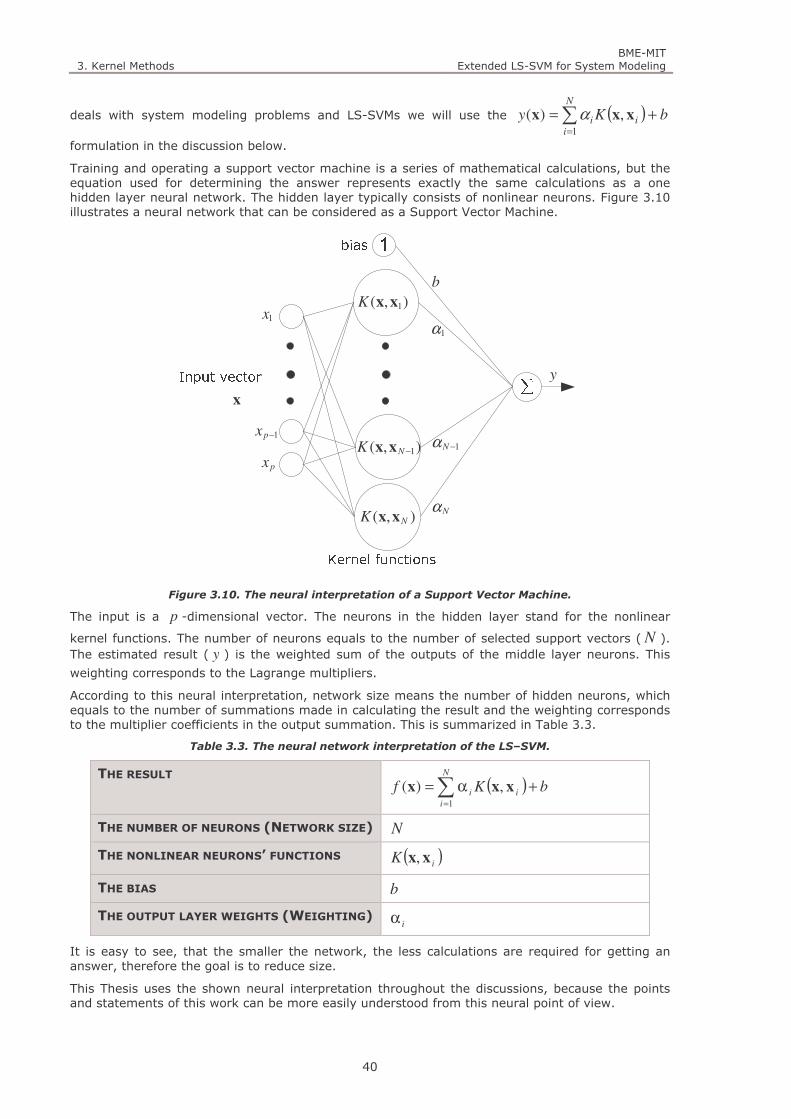
3. Kernel Methods BME-MIT
Extended LS-SVM for System Modeling
40
deals with system modeling problems and LS-SVMs we will use the ( ) bKy i
N
ii += ∑
=
xxx ,)(1
α
formulation in the discussion below.
Training and operating a support vector machine is a series of mathematical calculations, but the equation used for determining the answer represents exactly the same calculations as a one hidden layer neural network. The hidden layer typically consists of nonlinear neurons. Figure 3.10 illustrates a neural network that can be considered as a Support Vector Machine.
b
y
x
1x
px
1−px
),( 1xxK
),( 1−NK xx
),( NK xx
1α
1−Nα
Nα
Figure 3.10. The neural interpretation of a Support Vector Machine.
The input is a p -dimensional vector. The neurons in the hidden layer stand for the nonlinear
kernel functions. The number of neurons equals to the number of selected support vectors ( N ). The estimated result ( y ) is the weighted sum of the outputs of the middle layer neurons. This
weighting corresponds to the Lagrange multipliers.
According to this neural interpretation, network size means the number of hidden neurons, which equals to the number of summations made in calculating the result and the weighting corresponds to the multiplier coefficients in the output summation. This is summarized in Table 3.3.
Table 3.3. The neural network interpretation of the LS–SVM.
THE RESULT ( ) bKf i
N
i
i +α=∑=
xxx ,)(1
THE NUMBER OF NEURONS (NETWORK SIZE) N
THE NONLINEAR NEURONS’ FUNCTIONS ( )iK xx,
THE BIAS b
THE OUTPUT LAYER WEIGHTS (WEIGHTING) iα
It is easy to see, that the smaller the network, the less calculations are required for getting an answer, therefore the goal is to reduce size.
This Thesis uses the shown neural interpretation throughout the discussions, because the points and statements of this work can be more easily understood from this neural point of view.
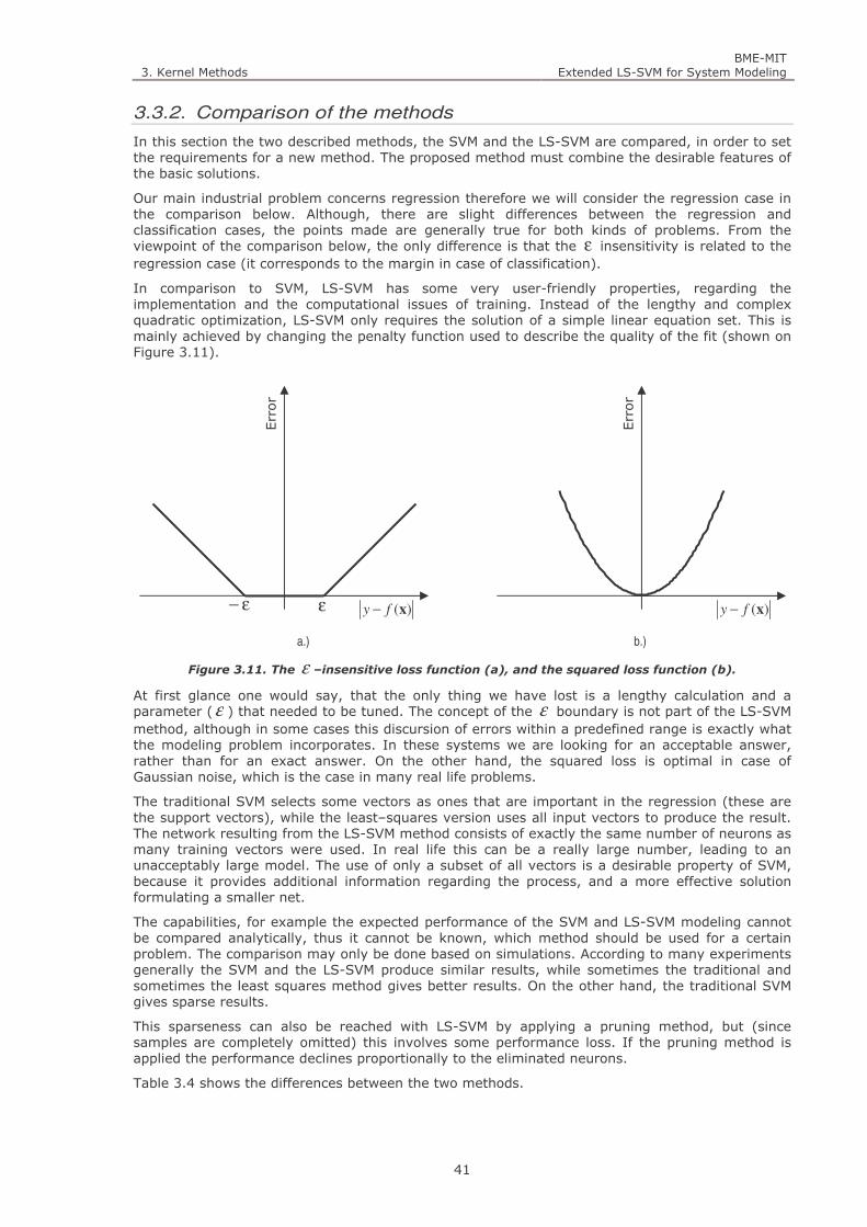
3. Kernel Methods BME-MIT
Extended LS-SVM for System Modeling
41
3.3.2. Comparison of the methods
In this section the two described methods, the SVM and the LS-SVM are compared, in order to set the requirements for a new method. The proposed method must combine the desirable features of the basic solutions.
Our main industrial problem concerns regression therefore we will consider the regression case in the comparison below. Although, there are slight differences between the regression and classification cases, the points made are generally true for both kinds of problems. From the viewpoint of the comparison below, the only difference is that the ε insensitivity is related to the regression case (it corresponds to the margin in case of classification).
In comparison to SVM, LS-SVM has some very user-friendly properties, regarding the implementation and the computational issues of training. Instead of the lengthy and complex quadratic optimization, LS-SVM only requires the solution of a simple linear equation set. This is mainly achieved by changing the penalty function used to describe the quality of the fit (shown on Figure 3.11).
a.) b.)
Figure 3.11. The ε –insensitive loss function (a), and the squared loss function (b).
At first glance one would say, that the only thing we have lost is a lengthy calculation and a parameter (ε ) that needed to be tuned. The concept of the ε boundary is not part of the LS-SVM method, although in some cases this discursion of errors within a predefined range is exactly what the modeling problem incorporates. In these systems we are looking for an acceptable answer, rather than for an exact answer. On the other hand, the squared loss is optimal in case of Gaussian noise, which is the case in many real life problems.
The traditional SVM selects some vectors as ones that are important in the regression (these are the support vectors), while the least–squares version uses all input vectors to produce the result. The network resulting from the LS-SVM method consists of exactly the same number of neurons as many training vectors were used. In real life this can be a really large number, leading to an unacceptably large model. The use of only a subset of all vectors is a desirable property of SVM, because it provides additional information regarding the process, and a more effective solution formulating a smaller net.
The capabilities, for example the expected performance of the SVM and LS-SVM modeling cannot be compared analytically, thus it cannot be known, which method should be used for a certain problem. The comparison may only be done based on simulations. According to many experiments generally the SVM and the LS-SVM produce similar results, while sometimes the traditional and sometimes the least squares method gives better results. On the other hand, the traditional SVM gives sparse results.
This sparseness can also be reached with LS-SVM by applying a pruning method, but (since samples are completely omitted) this involves some performance loss. If the pruning method is applied the performance declines proportionally to the eliminated neurons.
Table 3.4 shows the differences between the two methods.
)(xfy −
Error
)(xfy −ε
Error
ε−

3. Kernel Methods BME-MIT
Extended LS-SVM for System Modeling
42
Table 3.4. The comparison of the basic methods.
SVM LS-SVM
Support vectors are selected. All training vectors are considered.
Smaller network. Sparseness. Larger network. No sparseness.
Lengthy calculation (quadratic programming). Faster solution (linear equation set).
ε parameter. No ε parameter.
Iterative solution to make faster. Pruning method to reduce network size.
The starting point of our approach is the LS-SVM method, because our main goal is to handle large datasets, where the primary problem is the algorithmic complexity of the SVM. This is partly solved by the LS-SVM, but in case of huge datasets, even this problem formulation is too large. It is easy to see, that the kernel matrix (Ω ) must be created and stored (in the primary –not iterative- formulation) for both methods. To further reduce the complexity of the methods, the size of this matrix must be reduced!
It is easy to see, that an optimal solution should combine the desirable features of these methods.
3.3.3. Goals and exclusions
During the research, we have focused on four major issues of system modeling with LS-SVM, but there are still many related problems, research fields that are not or just merely addressed in this work. This section aims at defining the scope of this Thesis. For the issues not discussed in this work some starting points are provided too. The goals of this work:
Sparseness – create a simple model.
Good performance – to create a good, precise model.
Large scale methods – reducing algorithmic complexity.
Robust solution – reduce the effects of noise and outliers.
This work does not aim at solving the following problems:
Hyper parameter selection – Both SVM and LS-SVM construction (and of course almost all intelligent methods) involve some parameters, characterizing the model or the training process. In case of support vector methods, these hyper parameters are the following:
Kernel parameters (e.g. the σ in case of Gaussian kernel).
The C trade-off between the error and the model complexity.
ε defining the insensitivity zone for SVM regression.
Other parameters related to LS-SVM algorithms, e.g. defining the size of a pruned model in LS-SVM etc.
There are many papers concerning hyper parameter selection for both SVM and LS-SVM, for example see refs. [40]-[44].
Optimal implementation of basic methods – The methods presented in this Thesis also reduces the complexity of the LS-SVM training. The reduction described simplifies the problem formulation, by reducing the problem size. The discussion here focuses only on this problem size reduction, but it does not intend to offer the best algorithm or implementation to solve the specific problem.
Using prior information – There are many methods that aim at including some form of prior information, additional knowledge about the problem in the modeling process. In most cases this information is formulated as special kinds of rules. These rules are than built into the model construction, by applying some tricks, special methods. This Thesis focuses on traditional black-box modeling and does not examine the aspects of using prior information. There are points, where additional information is used about the complexity of the process, or the quality of the measurements, but no information is considered about the inside build-up or operation of the system.
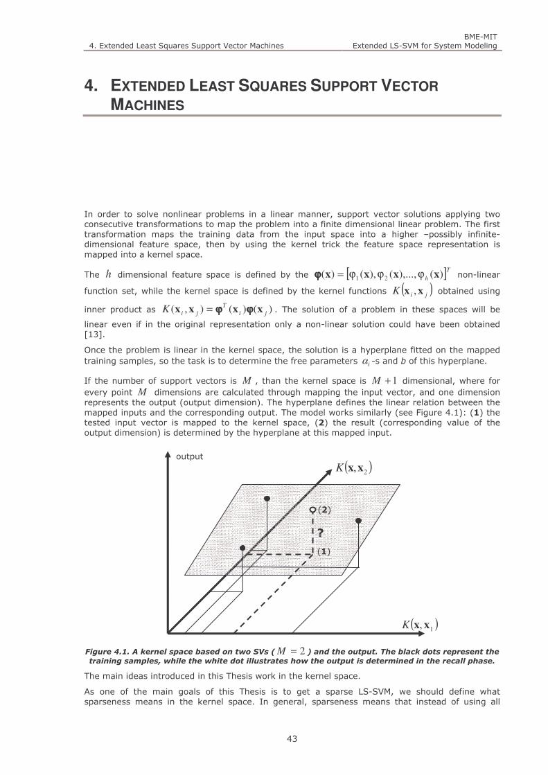
4. Extended Least Squares Support Vector Machines BME-MIT
Extended LS-SVM for System Modeling
43
4. EXTENDED LEAST SQUARES SUPPORT VECTOR
MACHINES
In order to solve nonlinear problems in a linear manner, support vector solutions applying two consecutive transformations to map the problem into a finite dimensional linear problem. The first transformation maps the training data from the input space into a higher –possibly infinite- dimensional feature space, then by using the kernel trick the feature space representation is mapped into a kernel space.
The h dimensional feature space is defined by the [ ]T
h )(),...,(),()( 21 xxxx ϕϕϕ=ϕϕϕϕ non-linear
function set, while the kernel space is defined by the kernel functions ( )jiK xx , obtained using
inner product as )()(),( ji
T
jiK xxxx ϕϕϕϕϕϕϕϕ= . The solution of a problem in these spaces will be
linear even if in the original representation only a non-linear solution could have been obtained [13].
Once the problem is linear in the kernel space, the solution is a hyperplane fitted on the mapped training samples, so the task is to determine the free parameters iα -s and b of this hyperplane.
If the number of support vectors is M , than the kernel space is 1+M dimensional, where for every point M dimensions are calculated through mapping the input vector, and one dimension represents the output (output dimension). The hyperplane defines the linear relation between the mapped inputs and the corresponding output. The model works similarly (see Figure 4.1): (1) the tested input vector is mapped to the kernel space, (2) the result (corresponding value of the output dimension) is determined by the hyperplane at this mapped input.
Figure 4.1. A kernel space based on two SVs ( 2=M ) and the output. The black dots represent the
training samples, while the white dot illustrates how the output is determined in the recall phase.
The main ideas introduced in this Thesis work in the kernel space.
As one of the main goals of this Thesis is to get a sparse LS-SVM, we should define what sparseness means in the kernel space. In general, sparseness means that instead of using all
?
( )1, xxK
( )2,xxKoutput
(2)
(1)

4. Extended Least Squares Support Vector Machines BME-MIT
Extended LS-SVM for System Modeling
44
training samples, only a subset, namely the support vectors are used. As the number of support vectors correspond to the number of kernels, this leads to a smaller model. In the kernel space the degree of sparseness is determined by the dimension of the hyperplane. If it is less than the number of training samples (this is the case in a traditional SVM) the solution will be sparse, while if the dimensionality of the hyperplane equals to the number of all training samples no sparseness is obtained. One major goal of this Thesis is to propose a new way of dimension-reduction which has only a limited effect on the performance of an LS-SVM. Another feature of the proposed approach is that it allows many different linear fitting strategies (or even a non-linear fit) in the kernel space, so the result will be not only sparse, but a simpler formulation, noise reduction and further reduction of algorithmic complexity can also be achieved while the quality is maintained. The unique feature of the propositions is that they start directly from the kernel space formulation.
When an LS-SVM is constructed from N training samples:
1. The training samples are mapped to an 1+N dimensional space, where N dimensions are defined by the kernel functions and one by the desired output.
2. In the 1+N -dimensional space an N -dimensional hyperplane is fitted on the mapped
samples. The free parameters of the hyperplane are determined by the N mapped training
points, and one additional constraint (∑=
=N
ii
1
0α ). For the sake of generalization and to
avoid overfitting the accuracy of the fit can be adjusted through regularization. To trade off between training error and a smooth solution the C (see (3.57)) regularization parameter is used, which is the same for all samples, and can be considered as a predefined, intentional error term in the kernel space fitting.
For a new sample x the response of the networks is determined by (3.62). This response is a point on the hyperplane and we expect that it will be close to the desired output. When a sparse solution is wanted only a subset of the training points are used to define the kernel space, thus the dimensions of both the kernel space and the hyperplane are reduced. However, due to this reduction some training points may fall far from the hyperplane, therefore the accuracy of the mapping decreases. The main problem is to reduce the number of dimensions without decreasing the accuracy. In dimension reduction some questions arise:
How many – and which – dimensions are needed in the kernel space? In a more definite form: can we use less than N dimensions, and how can the necessary dimensions be selected?
What is a good value of C , or more generally, how should the hyperplane be placed in the kernel space?
Having fewer dimensions in the kernel space results in a sparse solution, while an overdetermined equation set is obtained and this allows us to optimize the linear fit. This is illustrated in a simple example on Figure 4.2.

4. Extended Least Squares Support Vector Machines BME-MIT
Extended LS-SVM for System Modeling
45
a.) b.)
Figure 4.2. The image of training samples in a kernel space of different dimensions. Using all three
samples as support vectors (kernel centers), a three-dimensional kernel space guarantees exact fit
for the samples. The dashed lines represent a zone in which errors can be accepted (corresponding
to the ε -insensitivity of SVM).
Here the training points determine a hyperplane in the three-dimensional kernel space. In this kernel space all training points fit exactly the hyperplane. Reducing the dimension of this hyperplane we should select which training points will be used to define the two-dimensional hyperplane. The dimensionality of the kernel space is high enough, if samples (not used in determining this space) fall close (the error is acceptably small) to this plane after the mapping. Defining a tolerance interval one can decide if the dimension reduction can be allowed or not.
The proposed method has three main steps:
Using a special “partial reduction” technique, the LS-SVM training equation set is reformulated to describe a sparse model and algorithmically more effective problem (section 4.1).
In the second step, a new method is proposed to support the reduction, thus select the omitted data samples (section 4.5).
The reduced equation set can be solved using different ways to achieve more robust estimates (section 4.9).
4.1. Reduction methods
The starting point of our new approach is the linear equation set defined in (3.61) or (3.67) for regression or classification, respectively. The new approach may be similarly applied to both classification and regression problems, therefore we present the two versions in parallel. This section details the propositions of Thesis 1 (for the summary of the statements see section 8).
Using an overdetermined equation set
If the training set comprises N samples, then our original linear equation set consists of )1( +N
unknowns, the iα –s and the bias b , )1( +N equations and )1( +N 2 coefficients. These coefficients
are practically the values of the kernel function ( )ijK xx , . The number of training samples
therefore determines the size of the coefficient matrix, thus the number of unknowns, which has to be reduced in order to reduce network size and/or problem complexity.
Let’s take a closer look at the linear equation set describing both the classification and regression problems.
02
46
810
0
2
4
6
8
2
4
6
8
10
0 2 4 6 8 100
2
4
6
8
10
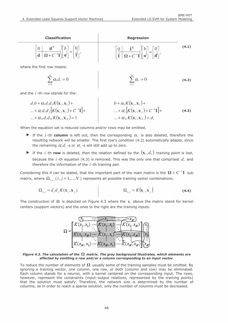
4. Extended Least Squares Support Vector Machines BME-MIT
Extended LS-SVM for System Modeling
46
Classification Regression
=
+ − 1αIΩd
dT
r00
1
b
C,
=
+ − dαIΩ1
1T 001
b
Cr
r
,
(4.1)
where the first row means:
∑=
=N
i
iid1
0α ∑=
=N
i
i
1
0α (4.2)
and the i -th row stands for the:
( )( )[ ]( ) 1,...
,...
,
1
111
=+
+++
++−
NiNiN
jijii
iii
Kdd
CKdd
Kddbd
xx
Ixx
xx
α
α
α
( )( )[ ]( ) iNiN
jii
i
dK
CK
Kb
=+
+++
++−
xx
Ixx
xx
,...
,...
,
1
11
α
α
α
(4.3)
When the equation set is reduced columns and/or rows may be omitted.
If the i -th column is left out, then the corresponding iα is also deleted, therefore the resulting network will be smaller. The first row’s condition (4.2) automatically adapts, since the remaining ii dα -s or iα -s will still add up to zero.
If the i -th row is deleted, then the relation defined by the ( )ii d,x training point is lost,
because the i -th equation (4.3) is removed. This was the only one that comprised id and therefore the information of the i -th training pair.
Considering this it can be stated, that the important part of the main matrix is the IΩ1−+ C sub
matrix, where ji ,Ω ( Nji ,...,1, = ) represents all possible training vector combinations.
),(, jijiji Kdd xx=Ω ( )jiji K xx ,, =Ω (4.4)
The construction of Ω is depicted on Figure 4.3 where the ix above the matrix stand for kernel
centers (support vectors) and the ones to the right are the training inputs.
Figure 4.3. The calculation of the Ω matrix. The gray background illustrates, which elements are
affected by omitting a row and/or a column corresponding to an input vector.
To reduce the number of elements of Ω usually some of the training samples must be omitted. By ignoring a training vector, one column, one row, or both (column and row) may be eliminated. Each column stands for a neuron, with a kernel centered on the corresponding input. The rows, however, represent the constraints (input–output relations, represented by the training points) that the solution must satisfy. Therefore, the network size is determined by the number of columns, so in order to reach a sparse solution, only the number of columns must be decreased.

4.
The following two reduction techniques can b
In order to reduce the network size and the complexity, the important samples must be kept, while the less significant ones may be omitted.
Traditional full redu
A training sample
to this sample are eliminated.
If full reduction is applied the solThe least noisy vectors seem to be the best choice. In this case however reduction also means, that the statistical characteristics owed to the numerous samples are p
The next equation demonstrates how the equation changes by fully omitting some training points. The deleted elements are
When traditional pruning pruning iteratively omits some trainipoints is entirely lost. To avoid this information loss, one may use the technique of partial reduction.
Proposed partial reduction
A training sample
but keeping the
of that row should still ad up to 1 (classification) or meat the
possible.
By selecting some (e.g. reduced, resulting in more equations than unknowns. The number of “support vectors” can be predetermined, but it can be a result of a selection method, like the one described in the next subsection. elements are
Since partial reduction is the main idea behind the extended LSpresented the method for both classification and regression. After presenting this very basic
Extended Least Squares Support Vector Machines
The following two reduction techniques can b
Full reduction
Partial reductionthe corresponding column, but keeping the row
In order to reduce the network size and the complexity, the important samples must be kept, while the less significant ones may be omitted.
Traditional full redu
training sample
to this sample are eliminated.
If full reduction is applied the solution– than these samples must be the ones representing the function as well as possible. The least noisy vectors seem to be the best choice. In this case however reduction also means, that the statistical characteristics owed to the numerous samples are p
The next equation demonstrates how the equation changes by fully omitting some training points. The deleted elements are
When traditional pruning pruning iteratively omits some trainipoints is entirely lost. To avoid this information loss, one may use the technique of partial reduction.
Proposed partial reduction
training sample
but keeping the
of that row should still ad up to 1 (classification) or meat the
possible.
By selecting some (e.g. reduced, resulting in more equations than unknowns. The number of “support vectors” can be predetermined, but it can be a result of a selection method, like the one described in the next subsection. The effect of this reduction is shown in the next equation, where the removed elements are colored
Since partial reduction is the main idea behind the extended LSpresented the method for both classification and regression. After presenting this very basic
nded Least Squares Support Vector Machines
The following two reduction techniques can b
Full reduction – a training sample
Partial reduction –
the corresponding column, but keeping the row
In order to reduce the network size and the complexity, the important samples must be kept, while the less significant ones may be omitted.
Traditional full reduction
training sample ( )ii y,x
to this sample are eliminated.
If full reduction is applied –than these samples must be the ones representing the function as well as possible.
The least noisy vectors seem to be the best choice. In this case however reduction also means, that the statistical characteristics owed to the numerous samples are p
The next equation demonstrates how the equation changes by fully omitting some training points. The deleted elements are colored
When traditional pruning [pruning iteratively omits some trainipoints is entirely lost. To avoid this information loss, one may use the technique of partial
Proposed partial reduction
training sample ( )ii y,x is only partially omit
but keeping the i -th row, which defines an input
of that row should still ad up to 1 (classification) or meat the
By selecting some (e.g. Mreduced, resulting in more equations than unknowns. The number of “support vectors” can be predetermined, but it can be a result of a selection method, like the one described in the next
The effect of this reduction is shown in the next equation, where the removed colored grey.
Since partial reduction is the main idea behind the extended LSpresented the method for both classification and regression. After presenting this very basic
nded Least Squares Support Vector Machines
The following two reduction techniques can b
a training sample
– a training sample
the corresponding column, but keeping the row
In order to reduce the network size and the complexity, the important samples must be kept, while the less significant ones may be omitted.
ction
is fully omitted, therefore both the column and the row corresponding
to this sample are eliminated.
–which means that only the remaining training samples will play part in than these samples must be the ones representing the function as well as possible.
The least noisy vectors seem to be the best choice. In this case however reduction also means, that the statistical characteristics owed to the numerous samples are p
The next equation demonstrates how the equation changes by fully omitting some training points. colored grey.
[22]-[25] is applied to the LSpruning iteratively omits some training points. The information embodied in the subset of dropped points is entirely lost. To avoid this information loss, one may use the technique of partial
Proposed partial reduction
is only partially omit
th row, which defines an input
of that row should still ad up to 1 (classification) or meat the
M , NM <reduced, resulting in more equations than unknowns. The number of “support vectors” can be predetermined, but it can be a result of a selection method, like the one described in the next
The effect of this reduction is shown in the next equation, where the removed
Since partial reduction is the main idea behind the extended LSpresented the method for both classification and regression. After presenting this very basic
nded Least Squares Support Vector Machines
47
The following two reduction techniques can be used on the regularized
a training sample ( )ii y,x
a training sample ( i ,x
the corresponding column, but keeping the row
In order to reduce the network size and the complexity, the important samples must be kept, while the less significant ones may be omitted.
is fully omitted, therefore both the column and the row corresponding
which means that only the remaining training samples will play part in than these samples must be the ones representing the function as well as possible.
The least noisy vectors seem to be the best choice. In this case however reduction also means, that the statistical characteristics owed to the numerous samples are p
The next equation demonstrates how the equation changes by fully omitting some training points. grey.
is applied to the LSng points. The information embodied in the subset of dropped
points is entirely lost. To avoid this information loss, one may use the technique of partial
is only partially omitted, by eliminating the corresponding
th row, which defines an input-output relation. It means, that the weighted sum
of that row should still ad up to 1 (classification) or meat the
) vectors as “support vectors”, the number of columns is reduced, resulting in more equations than unknowns. The number of “support vectors” can be predetermined, but it can be a result of a selection method, like the one described in the next
The effect of this reduction is shown in the next equation, where the removed
Since partial reduction is the main idea behind the extended LSpresented the method for both classification and regression. After presenting this very basic
47
e used on the regularized
) is fully omitted
)iy is only partially omitted, by only eliminating
the corresponding column, but keeping the row.
In order to reduce the network size and the complexity, the important samples must be kept,
is fully omitted, therefore both the column and the row corresponding
which means that only the remaining training samples will play part in than these samples must be the ones representing the function as well as possible.
The least noisy vectors seem to be the best choice. In this case however reduction also means, that the statistical characteristics owed to the numerous samples are p
The next equation demonstrates how the equation changes by fully omitting some training points.
is applied to the LS-SVM this is exactly the case, because ng points. The information embodied in the subset of dropped
points is entirely lost. To avoid this information loss, one may use the technique of partial
ted, by eliminating the corresponding
output relation. It means, that the weighted sum
of that row should still ad up to 1 (classification) or meat the
) vectors as “support vectors”, the number of columns is reduced, resulting in more equations than unknowns. The number of “support vectors” can be predetermined, but it can be a result of a selection method, like the one described in the next
The effect of this reduction is shown in the next equation, where the removed
Since partial reduction is the main idea behind the extended LSpresented the method for both classification and regression. After presenting this very basic
Extended LS
e used on the regularized Ω +
is fully omitted from both the column and row.
is only partially omitted, by only eliminating
In order to reduce the network size and the complexity, the important samples must be kept,
is fully omitted, therefore both the column and the row corresponding
which means that only the remaining training samples will play part in than these samples must be the ones representing the function as well as possible.
The least noisy vectors seem to be the best choice. In this case however reduction also means, that the statistical characteristics owed to the numerous samples are partially also lost.
The next equation demonstrates how the equation changes by fully omitting some training points.
SVM this is exactly the case, because ng points. The information embodied in the subset of dropped
points is entirely lost. To avoid this information loss, one may use the technique of partial
ted, by eliminating the corresponding
output relation. It means, that the weighted sum
of that row should still ad up to 1 (classification) or meat the iy (regression) goal, as closely as
) vectors as “support vectors”, the number of columns is reduced, resulting in more equations than unknowns. The number of “support vectors” can be predetermined, but it can be a result of a selection method, like the one described in the next
The effect of this reduction is shown in the next equation, where the removed
Since partial reduction is the main idea behind the extended LS-SVM the discussion above presented the method for both classification and regression. After presenting this very basic
Extended LS-SVM for System Modeling
I1−+ C matrix:
both the column and row.
is only partially omitted, by only eliminating
In order to reduce the network size and the complexity, the important samples must be kept,
is fully omitted, therefore both the column and the row corresponding
which means that only the remaining training samples will play part in than these samples must be the ones representing the function as well as possible.
The least noisy vectors seem to be the best choice. In this case however reduction also means, artially also lost.
The next equation demonstrates how the equation changes by fully omitting some training points.
SVM this is exactly the case, because ng points. The information embodied in the subset of dropped
points is entirely lost. To avoid this information loss, one may use the technique of partial
ted, by eliminating the corresponding
output relation. It means, that the weighted sum
(regression) goal, as closely as
) vectors as “support vectors”, the number of columns is reduced, resulting in more equations than unknowns. The number of “support vectors” can be predetermined, but it can be a result of a selection method, like the one described in the next
The effect of this reduction is shown in the next equation, where the removed
SVM the discussion above presented the method for both classification and regression. After presenting this very basic
BME-MITSVM for System Modeling
matrix:
both the column and row.
is only partially omitted, by only eliminating
In order to reduce the network size and the complexity, the important samples must be kept,
is fully omitted, therefore both the column and the row corresponding
which means that only the remaining training samples will play part in than these samples must be the ones representing the function as well as possible.
The least noisy vectors seem to be the best choice. In this case however reduction also means, artially also lost.
The next equation demonstrates how the equation changes by fully omitting some training points.
(4.5)
SVM this is exactly the case, because ng points. The information embodied in the subset of dropped
points is entirely lost. To avoid this information loss, one may use the technique of partial
i -th column,
output relation. It means, that the weighted sum
(regression) goal, as closely as
) vectors as “support vectors”, the number of columns is reduced, resulting in more equations than unknowns. The number of “support vectors” can be predetermined, but it can be a result of a selection method, like the one described in the next
The effect of this reduction is shown in the next equation, where the removed
(4.6)
SVM the discussion above presented the method for both classification and regression. After presenting this very basic
MIT SVM for System Modeling
both the column and row.
is only partially omitted, by only eliminating
In order to reduce the network size and the complexity, the important samples must be kept,
is fully omitted, therefore both the column and the row corresponding
which means that only the remaining training samples will play part in than these samples must be the ones representing the function as well as possible.
The least noisy vectors seem to be the best choice. In this case however reduction also means,
The next equation demonstrates how the equation changes by fully omitting some training points.
SVM this is exactly the case, because ng points. The information embodied in the subset of dropped
points is entirely lost. To avoid this information loss, one may use the technique of partial
th column,
output relation. It means, that the weighted sum
(regression) goal, as closely as
) vectors as “support vectors”, the number of columns is reduced, resulting in more equations than unknowns. The number of “support vectors” can be predetermined, but it can be a result of a selection method, like the one described in the next
The effect of this reduction is shown in the next equation, where the removed
SVM the discussion above presented the method for both classification and regression. After presenting this very basic

4. Extended Least Squares Support Vector Machines BME-MIT
Extended LS-SVM for System Modeling
48
concept, we restrict our discussion to the regression case, since our system modeling problem motivates this. The methods and extensions presented in the sequence can be applied to both cases. The discussion below basically focuses on two main topics:
How should the reduction be done? – (see section 4.2.2)
How can the reduced system be solved optimally? – (see section 4.9)
Both of these topics lead to results that work on the original or the reduced sets of equations, irrespective of their content (the problem they were derived from). Before going further to the selection problem or the possible solution schemes, some problems resulting from the proposed reduction must first be cleared. By deleting some columns from the quadratic matrices an MN ×rectangle matrix is attained, which raises the following questions:
Since the regularization is originally represented in the diagonal elements, the partial reduction results in an asymmetric matrix from this aspect. How does this effect the solution? How can this problem be resolved?
How can the constraint of the first row (4.2) be enforced in the overdetermined case (where there is no exact solution that satisfies all constraints)?
The answer to the second question is that this constraint is considered just like the others, as the solution to the overdertermined system consideres it similarly. This will of course not be exactly met, but this constraint does not seem to be extremely important. As it will be sown later, a more general formulation of this very same problem does not include this constraint.
In order to answer first questions let’s see a possible solution to the reduced problem.
Solving the partially reduced problem
As a consequence of partial reduction, our equation set becomes overdetermined, which can be solved as a linear least-squares problem (see Appendix 10.2.1), consisting of only M coefficients.
Let’s simplify the notations of our main equation as follows:
+=
redred
T
red
CIΩ1
1A 1
0r
r
,
=
red
b
αu ,
=
dv
0, (4.7)
where the index red means that the matrix is reduced ( redI also stands for a reduced unit matrix
containing an MM × unit matrix and MN − zero rows at the bottom). The solution will be:
vAu = → ( ) vAAAuTT 1−
= . (4.8)
This least squares solution is attained by multiplying this equation set
+
Ω
Ω
ΩΩ
=
∑
∑∑∑
=
=
==
2
2
1
,
1
,1
1
,
1
1,
100100
0011
110
CC
CC
CCN
N
i
iM
red
N
i
i
red
N
i
Mi
red
N
i
i
red
T
OM
L
M
L
ΩAA (4.9)
where (since red
T
redred
T
redCC
ΩIIΩ11
= )
red
T
redred
T
redC
IΩΩΩΩ1
2+= . (4.10)
4. Extended Least Squares Support Vector Machines BME-MIT
Extended LS-SVM for System Modeling
49
The right side of the equation set is
+
Ω
Ω=
∑
∑∑
=
=
=
MN
i i
Mi
red
N
i i
i
red
N
i i
T
dC
dC
d
d
d
1
1
0
1
1
,
1
1,
1
MMvA . (4.11)
It can be seen that due to the asymmetric regularization, the least squares solution takes a rather complicated form. On the other hand, if the terms affected by the regularization are handled separately, it can be seen, that the effect of the regularization is about the same as if it was
introduced after the matrix multiplication (the multiplication with TA ) as shown in ((4.12) and (4.13)). This can be justified as:
The second term of (4.9) is generally a regularization matrix, with a parameter 21
C. The
first column gives a small offset to the bias, while the first row (∑=
=N
i
i
1
0α ) disturbs the
constraint. This constraint does not really mean anything concerning the output of the model, especially in light of the fact that there is no constraint on the iα -s (any value , positive or negative is allowed). This constraint follows from the bias (see (3.60)), which is not essential to construct such a model. For example similar basis function models do not use a bias, while they are also universal approximators.
The term red
T
redC
IΩ1
in (4.10) can be considered as scaling up (weighting) the importance
of the support vectors, where the corresponding output is scaled similarly in (4.11).
To avoid this complex form the regularization term may be omitted from the kernel matrix, in which case the solution method applied to the overdetermined system should include some added constraint, most likely the minimization of the weight vector.
The most straightforward solution is to shift the regularization from the feature space to the kernel
space. This means that instead of minimizing w in the feature space, α will be minimized in
the kernel space. The linear equation set vAu = comprises
=
red
T
red
Ω1
1A r
r0
,
=α
ub
,
=
dv
0, (4.12)
and the solution will be
( ) vAIAAuTT
C1−
+= . (4.13)
The arguments above and simulation results both confirm that the regularization can be done in the kernel space, which provide a more friendly formulation. The effect of the regularization term is about the same, if the kernel space regularization term is the square of the one originally
used.(Feature space C
1 → Kernel space 21
C)
Sparse result
Now A is not a full rank matrix, as it has )1( +N rows and )1( +M columns. The deletion of
only columns with retaining the rows means that the number of neurons is reduced, but all the known constraints are taken into consideration. This is the key concept of keeping the quality,

4. Extended Least Squares Support Vector Machines BME-MIT
Extended LS-SVM for System Modeling
50
while the equation set is simplified. The answer of our model (in case of regression) takes the form:
( ) bKy i
M
i
i +α=∑=
xxx ,)(1
, svSi ∈ . (4.14)
where M is the cardinality of the support vector set svS containing the selected ix inputs.
In this way, the modified, reduced LS-SVM equation set can be solved in a least squared sense (in case of Gaussian noise), therefore we call this method Least Squares LS-SVM or shortly LS2–SVM.
The proposition presented here resembles to the basis of the Reduced Support Vector Machines (RSVM) introduced for standard SVM classification in ref. [60] (see section 3.1.6). The RSVM also selects a subset of the samples as possible delegates to be support vectors, but the selection method, the solution applied and the purpose of this reduction differs from the propositions presented. Since SVM is inherently sparse, the purpose of this selection is to reduce the algorithmic complexity, while our main goal is to achieve a sparse LS-SVM.
4.1.1. The kernel regularized LS-SVM
Let’s start from the same primal problem as described for the LS-SVM. The equation
∑=
+=N
i
iT
beCJ
1
2
,, 2
1
2
1),(min wwew
ew, (4.15)
with constraints:
( ) iiT
i ebd ++= xw ϕϕϕϕ , Ni ,...,1= . (4.16)
(see also (3.57),(3.58)) defines the problem in the feature space, where the first ww T
21 term is
the regularization term, which in case of SVM corresponds to the margin maximalization. This also means that a C trade-of parameter is also introduced in the feature space. It was shown (in section 3.2) that this parameter becomes a term in the diagonal of the main matrix of the final equation set (see equation (3.61)), which means that a quadratic kernel matrix is used. As long as the kernel matrix is quadratic our solution cannot be sparse since all training samples contribute a kernel.
If we omit the minimization of w from the feature space, thus remove the first term, the
equation becomes a classical least-squares regression:
( )∑=
−+=N
i
iiT
bdbeJ
1
2
,)(),(min xww
wϕϕϕϕ . (4.17)
Let w be of the form:
∑=
=M
j
jj
1
)(xw ϕϕϕϕα . (4.18)
where NM < vectors are the “support vectors”. Since the number of the iα variables are
reduced, this leads to more equations than unknowns.
Defining w as a linear combination of the feature vectors can be justified using equations (3.59) and (3.60) formulated for M training samples. If equation (3.59) defines the optimization
problem for the NM < samples than the 0w
=∂
∂L criteria concludes to (4.18). This means, that
4. Extended Least Squares Support Vector Machines BME-MIT
Extended LS-SVM for System Modeling
51
w is determined by a smaller sample set (the support vectors), while the constraints represent a larger training set.
If we plug this into (4.17) and apply the kernel trick we get an overdetermined linear equation set (see equation (4.21)). This equation set is detailed in the next section, where the least-squares solution is introduced.
It is easy to see, that this equation set is almost the same as the one achieved through “partial reduction”. There are two differences:
The ∑=
=N
i
i
1
0α condition is not incorporated.
As described earlier (in section 4.1) this condition is not considered to be important, but in order to include this; it can be added to the equation set afterwards.
There is no regularization in this formulation.
As we have shown earlier, the regularization can be introduced in the kernel space. If the error measure used is not a least-squares error than the overdetermined equation set is not solved in a least-squares sense, therefore in this case, the regularization is replaced by some other optimization scheme, for example weighting (this described in the section 4.9, where the robust solutions are introduced).
Limiting the number of iα weights is the key concept to get a sparse model, but as we keep all
the training samples this does not constrain our optimization to the corresponding support vector set as in traditional LS-SVM pruning. This reduces the kernel matrix, where the deletion of only columns with retaining the rows means that the number of kernels is reduced, but all the known constraints are taken into consideration. This is the key concept of keeping the quality, while the equation set is simplified.
This method is called partial reduction, since it reduces the number of support vectors, but keeps all the samples as constraints (see (4.6)). From this viewpoint it can also be seen, why the regularization was removed. If we remove a column from the kernel matrix, the regularization term will be missing from the i -th row, which results in an asymmetric formulation. By removing
the regularization (the wwT
2
1 term) this asymmetry is eliminated.
4.1.2. The least-squares solution (LS2-SVM)
The least-squares solution presented in this section has already been introduced when partial reduction was described. The reason to describe this solution in that context was to show that the overdetermined equation set resulting from the proposed reduction can be solved. It is also shown, that the regularization may be shifted from the feature space to the kernel space. This lead to a forward derivation of the same method, namely to the kernel regularized LS-SVM.
The least squares solution is detailed here because this is the most basic and most important solution method for the introduced sparse (partially reduced) LS-SVM formulations. It must also be emphasized, if no reduction is used, this method is exactly equivalent with the original LS-SVM solution.
Usually there are two important assumptions that are made about the noise ( z ):
The noise exists only on the output.
The noise is random and follows a normal (Gaussian) distribution with zero mean and
constant variance 2σ .
In this case the summed square of the residuals must be minimized:
∑=
+−=M
j
ijjii bKde1
),( xxα , (4.19)

4. Extended Least Squares Support Vector Machines BME-MIT
Extended LS-SVM for System Modeling
52
∑ ∑∑= ==
+−==N
i
M
j
ijji
N
i
bKdeS i
1
2
11
2 )),(( xxα . (4.20)
The solution of equation (4.20) can be formulated as
=
α
α
N
M
NMN
M
d
db
KK
KK
MM
L
MOMM
L 1
1
1
111
),(),(1
),(),(1
xxxx
xxxx
. (4.21)
Let’s simplify the notations as follows:
[ ]Ω1A = ,
=α
ub
, dv = . (4.22)
Than the least squares solution is:
vAuAA TT =)( . (4.23)
Instead of this, the regularized least-squares solution is used, to minimize the α :
vAuIAA TTC =+ − )( 1
. (4.24)
The modified matrix A has )(N rows and )1( +M columns. After the matrix multiplications the
results are obtained from a reduced equation set, incorporating AAT , which is of size
)1()1( +×+ MM only. The result of this matrix multiplication may be interpreted as a mapping,
which maps the problem into a hyper kernel space.
4.1.3. Sparseness and performance
On the performance of a model (modeling approach) we mean the quality of the estimation, thus the true risk. The sparseness and performance properties of a model are still related. It is likely that a sparser model (containing less SVs) has worse performance than a larger one.
As discussed earlier in section 3.2.3 the sparse LS-SVM is achieved by disregarding some of the training samples, and using only a subset as training set. This method has been discussed as full reduction in section 4.1. By using only part of the training samples, some information is lost, consequently the model performance may decline, errors may grow. The proposed partial reduction enables us to create a sparse model, while all available training samples are considered. This improves model performance, since the result is based on all the information.
The sparseness and performance properties of a model are still related. A sparser model (containing less support vectors) is likely to have worse performance than a larger one.
Comparing the traditional pruning method (full reduction) to partial reduction, there are two statements that can be made:
The partial reduction can produce similar performance with smaller network.
With the same network size, the partially reduced solution can provide better performance.
In most practical applications these differences are very significant, that would lead to unacceptably large errors if the model is created using full reduction. This will be demonstrated in the experiments section (see section 5).

4. Extended Least Squares Support Vector Machines BME-MIT
Extended LS-SVM for System Modeling
53
4.2. Related works concerning reduction
In this section we summarize two methods from the literature, that use similar reduction as proposed.
The first method is the Reduced Support Vector Machine (RSVM) [60] which uses a random support vector selection method to reduce algorithmic complexity of the SVM. Since the SVM is inherently sparse, the only goal of this method is to provide a fast -but still good- solution.
The Reduced Rank Kernel Ridge Regression (RRKRR) [63],[64] aims at a sparse result and introduces the same idea as partial reduction. Although this method almost exactly corresponds to our proposition, there are some important differences (see the remarks in section 4.4).
4.2.1. Reduced Support Vector Machines
The RSVM method generates the separating surface such, that the model is based on as little as 1% of a large dataset. To generate this nonlinear surface, the entire dataset is used as a constraint in an optimization problem with a small number of variables corresponding to the data kept. This is achieved by making use of a rectangular NM × kernel matrix Ω (see equation (3.35)) that greatly reduces the size of the quadratic program to be solved and simplifies the characterization of the nonlinear separating surface. Here, the N rows of Ω represent the original n data points while the M columns stand for the greatly reduced data points taken as SV delegates. The data points used for generating the columns are selected randomly. In order to solve such a rectangular system, the SVM problem is converted into an equivalent SSVM which is an unconstrained optimization problem.
Experimental results indicate that test set correctness for the reduced support vector machine (RSVM), with a nonlinear separating surface that depends on a small randomly selected portion of the dataset, is better than that of a conventional support vector machine (SVM) with a nonlinear surface that explicitly depends on the entire dataset, and much better than a conventional SVM using a small random sample of the data. Both time and memory complexity are much smaller for RSVM than those of a conventional SVM using the entire dataset.
4.2.2. Reduced Rank Kernel Ridge Regression
In the original ridge regression the kernel matrix is quadratic which means, that the final result is based on as many support vectors, as many training samples are used (see equation (10.25)), thus it is not sparse. The Reduced Rank Kernel Ridge Regression published in 2002 proposes a way to solve this problem by reducing the dimensionality of the kernel space. The results are presented with the bias, similarly to the LS-SVM formulation.
The model implemented by the LS-SVM is given by
The optimal values for the weight vector and the bias are obtained by determining the minimum of
By defining the corresponding dual formulation the solution – the α and the bias b – is calculated from a set of linear equations.
To achieve a sparse solution one has to reduce the number of kernels. This can be obtained by using only the important subspace of the feature space, which can be used to generate the kernel
space. The feature space – or it’s “important” subspace – is span by the feature vectors )( ixϕϕϕϕ ,
therefore by selecting a basis from these vectors, a compact representation is gained.
bKfN
i
ii
T +α== ∑=1
),()()( xxxwx ϕϕϕϕ . (4.25)
∑=
−−+=N
i
iT
i bdCbJ1
22))((
2
1),( xwww ϕϕϕϕ . (4.26)
4. Extended Least Squares Support Vector Machines BME-MIT
Extended LS-SVM for System Modeling
54
If the weight vector w can be represented as a weighted sum of the basis vectors (the set S contains the indices of the input samples comprised in the basis):
then the objective function of RRKRR becomes:
Setting the partial derivatives by β and b to zero and dividing by C2 the conditions of optimality
are:
and for Sr ∈∀
Equations (4.29) and (4.30) lead to the a linear equation set of size )1()1( +×+ SS .
The result of this equation set leads to a reduced rank – sparse - solution, since it only contains
the sum of S kernels and the bias. It can be seen that this method (besides the form of the final
equation set) corresponds to the kernel regularized LS-SVM described in section 4.1.1.
4.3. Discussion on reduction methods
To discuss the motivations to use partial reduction and its advantages over traditional methods, a short overview of the main idea and sparse LS-SVM must be given, from some new perspectives.
If the problem can be solved with M ( NM << ) kernels (neurons) than the model constructed should not contain more. In the case of LS-SVM the model size equals to the number of training
∑∈
=Si
ii )(xw ϕϕϕϕβ (4.27)
∑ ∑∑= ∈∈
−−+=N
i Sj
jiji
Sji
jiji bKdCKbJ1
2
,
)),((),(2
1),( xxxxβ βββ . (4.28)
∑∑ ∑=∈ =
=+N
j
j
Si
N
j
jii dbK11
),( xxβ (4.29)
∑∑∑ ∑==∈ =
=+
+
N
j
rij
N
i
ri
Si
N
j
ijrjrii KdKbKKKC 111
),(),(),(),(),(2
1xxxxxxxxxxβ . (4.30)
=
∑ =
N
kkdbN
1
cβΦ
ΦΩ,
where the SS ×
Ω matrix, Φ and c vectors (of S elements) are built from the
elements:
∑=
+=ΩN
j
ijrjriir KKKC 1
, ),(),(),(2
1xxxxxx , Sri ∈,
∑=
=N
irir KΦ
1
),( xx , Si ∈∀
∑=
=N
j
rijr Kdc1
),( xx Si ∈∀
(4.31)
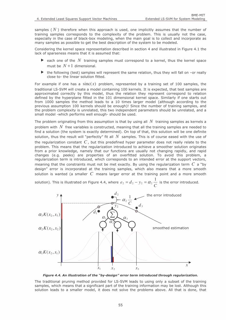
4. Extended Least Squares Support Vector Machines BME-MIT
Extended LS-SVM for System Modeling
55
samples ( N ) therefore when this approach is used, one implicitly assumes that the number of training samples corresponds to the complexity of the problem. This is usually not the case, especially in the case of black-box modeling, when the main goal is to collect and incorporate as many samples as possible to get the best description of the system to be modeled.
Considering the kernel space representation described in section 4 and illustrated in Figure 4.1 the lack of sparseness means that it is assumed that:
each one of the N training samples must correspond to a kernel, thus the kernel space
must be 1+N dimensional.
the following (test) samples will represent the same relation, thus they will fall on –or really close to- the linear solution fitted.
For example if one has a )sinc(x problem, represented by a training set of 100 samples, the
traditional LS-SVM will create a model containing 100 kernels. It is expected, that test samples are approximated correctly by this model, thus the relation they represent correspond to relation defined by the hyperplane fitted in the 101 dimensional kernel space. Similarly if one starts out from 1000 samples the method leads to a 10 times larger model (although according to the previous assumption 100 kernels should be enough)! Since the number of training samples, and the problem complexity is unrelated, this two independent parameters should be unrelated, and a small model -which performs well enough- should be used.
The problem originating from this assumption is that by using all N training samples as kernels a
problem with N free variables is constructed, meaning that all the training samples are needed to find a solution (the system is exactly determined). On top of that, this solution will be one definite solution, thus the result will “perfectly” fit all N samples. This is of course eased with the use of
the regularization constant C , but this predefined hyper parameter does not really relate to the problem. This means that the regularization introduced to achieve a smoother solution originates from a prior knowledge, namely that our functions are usually not changing rapidly, and rapid changes (e.g. peeks) are properties of an overfitted solution. To avoid this problem, a regularization term is introduced, which corresponds to an intended error at the support vectors, meaning that the constraints must not be met exactly. By using the regularization term C a “by design” error is incorporated at the training samples, which also means that a more smooth solution is wanted (a smaller C means larger error at the training point and a more smooth
solution). This is illustrated on Figure 4.4, where C
yde1
2222 α=−= is the error introduced.
Figure 4.4. An illustration of the “by-design” error term introduced through regularization.
The traditional pruning method provided for LS-SVM leads to using only a subset of the training samples, which means that a significant part of the training information may be lost. Although this solution leads to a smaller model, it does not solve the problems above. All that is done, that
1α2α
3α
C
12α
smoothed estimation
the error introduced
1x 2x 3x
1d
2d
3d2y
x
y
),( 121 xxKα
),( 222 xxKα
),( 323 xxKα ∑
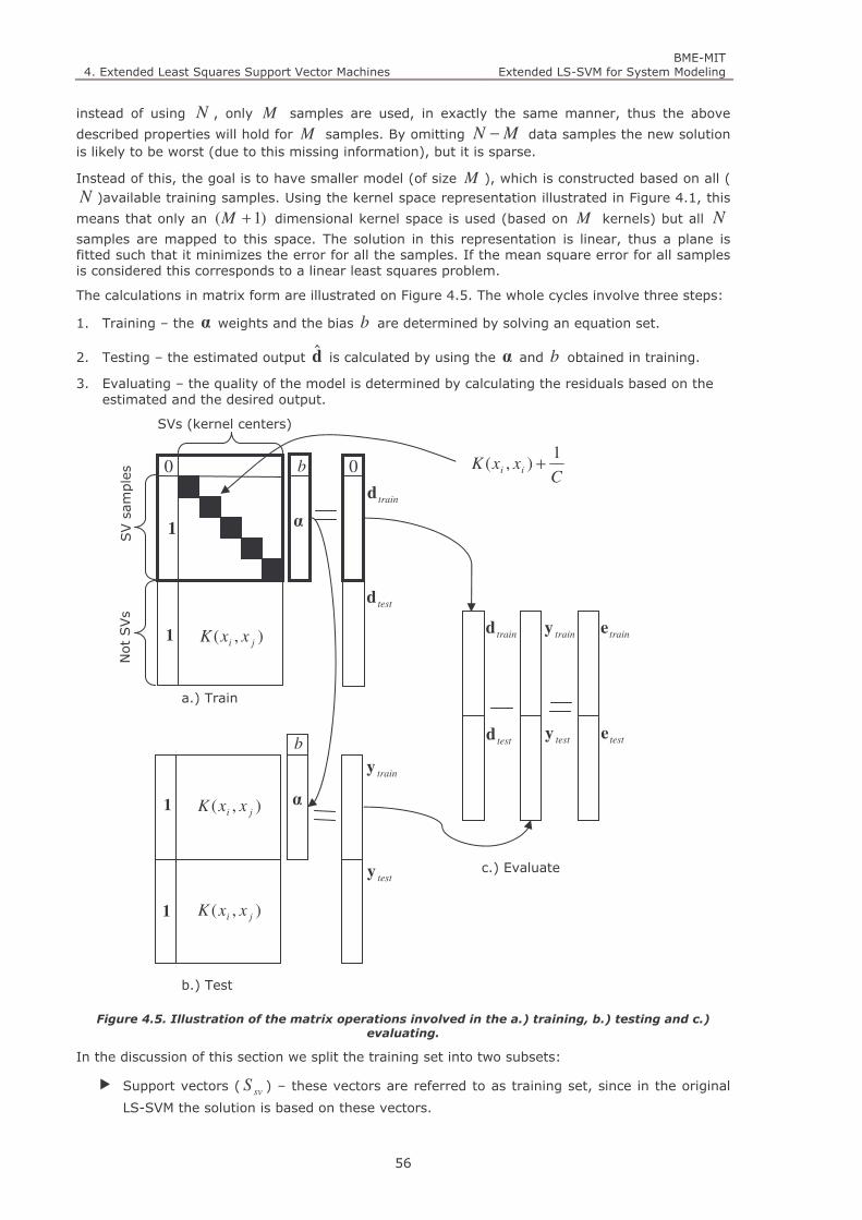
4. Extended Least Squares Support Vector Machines BME-MIT
Extended LS-SVM for System Modeling
56
instead of using N , only M samples are used, in exactly the same manner, thus the above
described properties will hold for M samples. By omitting MN − data samples the new solution is likely to be worst (due to this missing information), but it is sparse.
Instead of this, the goal is to have smaller model (of size M ), which is constructed based on all (N )available training samples. Using the kernel space representation illustrated in Figure 4.1, this
means that only an )1( +M dimensional kernel space is used (based on M kernels) but all N
samples are mapped to this space. The solution in this representation is linear, thus a plane is fitted such that it minimizes the error for all the samples. If the mean square error for all samples is considered this corresponds to a linear least squares problem.
The calculations in matrix form are illustrated on Figure 4.5. The whole cycles involve three steps:
1. Training – the α weights and the bias b are determined by solving an equation set.
2. Testing – the estimated output d is calculated by using the α and b obtained in training.
3. Evaluating – the quality of the model is determined by calculating the residuals based on the estimated and the desired output.
Figure 4.5. Illustration of the matrix operations involved in the a.) training, b.) testing and c.)
evaluating.
In the discussion of this section we split the training set into two subsets:
Support vectors ( svS ) – these vectors are referred to as training set, since in the original
LS-SVM the solution is based on these vectors.
testd
a.) Train
b.) Test
SV sam
ples
Not SVs
SVs (kernel centers)
c.) Evaluate
b
b
α
α
traind
testd
trainy
testy
CxxK ii
1),( +
),( ji xxK
),( ji xxK
),( ji xxK
traind trainy
testy
traine
teste
00
1
1
1
1

4. Extended Least Squares Support Vector Machines BME-MIT
Extended LS-SVM for System Modeling
57
Non support vectors ( svnonS − )– these samples can be considered as test samples, since in
the original LS-SVM these samples can only be used for testing. These test samples are not the same as the ones originally in the test set described in section 2.
If partial reduction is applied, the rows of the reduced kernel matrix can be rearranged to have the rows corresponding to the support vectors on the top and in the proper order. This way, the regularization is moved to the upper part of the rectangular kernel as shown in Figure 4.5.
In case of the original LS-SVM, only the square upper part is used (marked with a thick line on Figure 4.5) and training means that this equation set is solved. Since this equation set is quadratic, there is one exact solution where the error for a given sample (support vector) corresponds to
kkC
e α= 1
. (4.32)
The results for the non-support vectors can be determined by
( ) bKy i
M
i
i +α=∑=
xxx ,)(1
, svSi ∈ , (4.33)
thus by matrix multiplication for the bottom part of the matrix on Figure 4.5 a.) and b.).
Experiments show that usually –if C is not determined properly – the errors ( iii yde −= ,
svnonSi −∈ ) for the non-SVs (test vectors) are usually larger than the errors for the support vectors. This is the consequence of having an exactly determined system containing only the SVs as training information. If only the selected M constraints are considered (see section 3.2.3 and Figure 3.7 for details), the C hyper parameter must be chosen such that according to (4.32) the errors correspond to the errors for the test samples (the non support vectors). Thus by a proper selection of C overfitting can be omitted, since this regularization parameter can introduce errors at the training samples, since it disturbs the constraints of the training equation set. Since the whole training set is available for creating the model, it is reasonable to have a model satisfying all the samples equally well (have about the same error for the training and test samples). This can be done through tuning C using cross validation (see section 2.3.1), which is generally a very lengthy process requiring many training and testing iterations.
The idea of partial reduction can be viewed as doing cross-validation in one step, optimizing for the support vectors (as a training set) and the non support vectors (as a test set) at the same time. Instead of solving the upper LS-SVM square equation set with different C settings validated
on the bottom part of the equation set (the non support vectors) iteratively, until a proper C is found (e.g. the error equals for the upper-training and bottom-testing part), this is done in one step, by solving the overdetermined equation set in a least squares sense. This way the resulting α weights and the bias b will be optimal for the whole equation set (more precisely the mean square error will be minimal for the whole training sample set, thus for the union of the SVs and non SVs).In this case the summed square of the residuals for the whole training set is minimized:
∑ ∑∑= ==
+−==N
i
M
j
ijji
N
i
bKdeS i
1
2
11
2 )),(( xxα . (4.34)
The least squares approximation provides the optimal solution, thus it minimizes this error (see Appendix 10.2.1), therefore - as far as this error is considered - this solution guaranties the best approximation.
It is also important to emphasize, that by baseing the solution on only a subset of the samples the solution can only satisfy the constraints defined by these samples. To avoid overfitting to this training set a smoothing regularization term (C ) is introduced. This can lead to having a larger error at the support vectors and a smaller error for the non support vectors, but if an important training sample is omitted, this information cannot be recovered (see Figure 4.6).

4. Extended Least Squares Support Vector Machines BME-MIT
Extended LS-SVM for System Modeling
58
Figure 4.6. Illustration of information loss in case of full reduction The effect of regularization is
also illustrated. For the dotted line a larger regularization (smaller C ) is used.
This means, that by adjusting the regularization the errors may be equilibrated for the SV and non-SV samples, but this error cannot be less – and if a significant sample is dropped (marked with a “!” in Figure 4.6), it is necessarily larger – than the error of the least squares approximation, based on the overdetermined equation set, which mathematically provides a true minimum (for the error defined in equation (4.34)).
4.4. Remarks on reduction
Partial reduction uses a combination of two possible SRM structures (2.17) and (2.19) (see section 2.4), since the reduction (aimed at achieving sparseness) uses the first SRM structure, since it eliminates basis functions, while (after having a fixed kernel number) in the latter steps it also minimizes the parameter vector corresponding to w .
The reduced rank kernel ridge regression formulation was developed and published parallel to the proposed partial reduction (LS2-SVM) in 2002. These methods lead to almost the same results, although they where derived from two different aspects. The RRKRR is based on an effective representation of the feature space, the LS2-SVM achieves a sparse model by reducing the equivalent kernel space representation. Another important difference is that the two models were derived from different theoretical backgrounds.
While most known methods work in the primal, or –when the problem is nonlinear- in the feature space propositions of this Thesis work primarily in the kernel space. This is emphasized throughout this work, because the basic idea is to take the kernel based formulation of the problem – consider it equivalent to the primal problem- and try optimizing this according to the goals (e.g. sparseness, robustness). The way of achieving a sparse model requires two steps:
The model size must be reduced, by selecting support vectors.
The corresponding optimization problem must be formed and solved.
The task of selecting some vectors as support vectors, can be done successfully in the primal-, the feature- and in the kernel space, since the result of this selection can be used even after the next transformation.
If the second task is formed in the feature space, like in the RRKRR case, the optimization problem leads to a quadratic kernel space formulation – a quadratic linear problem- allowing only one solution. In the RRKRR case the error norm (least squares error) is determined in the feature space formulation, which leads to only one unique solution which minimizes this error. In case the reduction is done directly on the kernel space formulation, the resulting optimization problem –formed as an overdetermined linear equation set- is in the kernel space, therefore arbitrary error measures (e.g. loss functions) may be used –and a corresponding optimal solution may be found- without rewriting the problem in the feature space. The details on this will be discussed in section 4, where we propose to use this approach, and describe methods based on this formulation. It is also shown, that the least squares solution, applied to the kernel space problem, can be related to RRKRR (which achieves this through a feature space formulation).
If the training set comprises N points, than the equation set consists of 1+N equations,
meaning that the size of the matrix to be manipulated is )1()1( +×+ NN . As usually
1>>N , to keep the formulas simple we will consider a matrix of size NN × .
1C
2C
12 CC <
!
4. Extended Least Squares Support Vector Machines BME-MIT
Extended LS-SVM for System Modeling
59
Considering one multiplication and one addition as an operation. The complexity of solving the partially reduced system [66]-[69]:
Multiplying of the left side by TA ( AA
T in eq. (4.8)): NM2
Multiplying of the right side by TA ( vAT in eq. (4.8)): NM
Solving the linear equation set using the LU decomposition: 23
3
1MM + . Where the
LU decomposition means 3
3
1M steps, while the back substitution to determine the
unknowns costs 2M . (The currently available best algorithm for matrix inversion is
)( 376,2MO [68]. In this case the result is calculated from a matrix multiplication (
bA 1− ) requiring an additional 2M steps.)
Therefore for a fixed M ( NM << ) the solution is linear in N , supposing that the reduction (support vector selection) requires no computation (e.g. random selection). It is important to emphasize, that the primary goal of the described method is not an algorithmic gain, rather to achieve a sparse, and still precise solution.
4.5. Support Vector selection
In the neural interpretation, every Lagrange multiplier )( kα belongs to a neuron –representing
it’s weight– and each of the M selected training vectors will become a centre of a kernel function, therefore the selected inputs must be chosen accordingly. If the above described overdetermined solution is used, than the following question must be answered: How many and which vectors are needed?
Standard SVM automatically marks a subset of the training points as support vectors. With LS-SVM one has a linear equation set which has to be reduced to an overdetermined equation set in such a way, that the solution of this reduced problem is the closest to what the original solution would be. For this purpose two new methods are proposed, a Reduced Rank Echelon Form (RREF) based method, and the inverse pruning method.
The selection methods described in this section are summarized by Thesis 2 (see section 8).
4.5.1. The RREF method for SV selection
The problem is to find a selection method to determine the vectors for the reduced equation set. The whole reduction method can be interpreted in the following way.
As the matrix is formed from columns we can select a linearly independent subset of column vectors and omit all others, which can be formed as linear combinations of the selected ones. This can be done by finding a “basis” (the quote indicates, that this basis is only true under certain conditions defined later) of the coefficient matrix, because the basis is by definition the smallest set of vectors that can solve the problem. This basis can be found by a slight modification of a common mathematical method used for bringing the matrix to the reduced row echelon form (see Appendix 10.4), using Gauss-Jordan elimination with partial pivoting [66],[69]. This is discussed in more detail in the sequel.
The basic idea of doing a feature selection in the kernel space is not new. The nonlinear principal component analysis technique, the Kernel Principal Component Analysis (Kernel PCA) uses a similar idea [70]-[73]. One difference should be emphasized. Most of the methods formulate the problem and the optimization in he primal or in the feature space, and then solve it in the kernel space. The propositions of this Thesis consider the kernel space formulation of the problem as a new transformed, but equivalent representation of the original problem and solve this problem directly. The selection of a basis to represent the linearized (feature) space has been shown in ref. [74]. This paper operates in the kernel space, to construct the basis of the feature space (see section 4.6.2).

4. Extended Least Squares Support Vector Machines BME-MIT
Extended LS-SVM for System Modeling
60
This reduced input set (the support vectors) is (are) selected automatically by determining a
“basis” of the Ω (or the IΩ1−+ C ) matrix. Let’s examine this a little closer!
An vAu = linear equation set may be viewed as follows: if we consider the columns of A , than v is formed as the weighted sum of these vectors. The equation set has a solution if and only if v is in the span of the columns of A . Every solution (u ) means a possible decomposition of v into these vectors, but an LS-SVM problem requires only one(!). The solution is unique if and only if the columns of A are linearly independent. This means that by determining a basis of A –any set of vectors, that are linearly independent, and span the same space as A – the problem can be reduced to a weighted sum of fewer vectors.
In this proposed solution however, a columnvector is considered to be linearily dependent of the others it can be constructed with only a small error as a linear combination of them. This is
illustrated on Figure 4.7, where the 5u vector can be constructed from the first four columns (a.),
but if some error is acceptable, the first three vectors may be enough (b.).
Figure 4.7. Constructing a vector as a linear combination.
In order to achieve this, the method uses an adjustable tolerance parameter when determining the “resemblance” of the column vectors. The use of this tolerance value is essential, because none of the columns of Ω will likely be exactly dependent of the others, especially if the selection is
applied to the regularized IΩ1−+ C matrix. This tolerance ( ε′ ) can be related to the ε
parameter of the standard SVM, because it has similar effects. The larger the tolerance, the fewer vectors the algorithm will select. If the tolerance is chosen too small, than a lot of vectors will seem to be independent, resulting in a larger network. As stated earlier the standard SVM’s sparseness is due to the ε –insensitive loss function, which allows the samples falling inside this insensitive zone to be neglected. It may not be very surprising to find, that an additional parameter is needed to achieve sparseness in LS-SVM. This parameter corresponds to ε , which was originally left when changing from the SVM to the standard least-squares solution.
This selection process incorporates a parameter which indirectly controls the number of resulting basis vectors (M ). This number does not really depend on the number of training samples ( N ), but only on the problem, since M only depends on the number of linearly independent columns. In practice it means that if the problem’s complexity requires M neurons, than no matter how many training samples are presented, the size of the resulting network does not change.
The reduction is achieved as a part of transforming the TA matrix into reduced row echelon form
[69],[76]. The tolerance is used in the rank tests. The algorithm uses elementary row operations:
1. Interchange of two rows.
2. Multiply one row by a nonzero number.
3. Add a multiple of one row to a different row.
The algorithm is a slight modification of the Gauss-Jordan elimination with partial pivoting and goes as follows ( i -row index, j -column index) [66],[67]:
1. Loop over the entire matrix, working down the main diagonal starting at row one, column one.
2. Determine the largest element p in column j with row index ji ≥ .
a.) b.)
5u1u
2u
3u4u
5u1u
2u
3u

4. Extended Least Squares Support Vector Machines BME-MIT
Extended LS-SVM for System Modeling
61
3. If ε ′≤p (where ε′ is the tolerance parameter) then zero out the remainder of the column
(elements in the j -th column with index ji ≥ );
else remember the column index because we found a basis vector (support vector), exchange the rows to have the largest element in the working (pivot) position (in the main diagonal), divide the row with the pivot element p (to have 1-at the working position) and
subtract multiples of the row from all other rows, to attain 0-s in the column (above and bellow, the working position).
4. Step forward to 1+= ii and 1+= jj . Go to step 1.
∗
∗∗∗∗∗∗∗∗∗∗
LL
MOMMMM
L
L
L
L
mp
p
p
00
00
001001
2
1
Figure 4.8. An intermediate step of the Gaussian elimination with partial pivoting (the ip elements
are the delegates to become the next pivot element).
This method returns a list of the column vectors which are linearly independent form the others considering tolerance ε′ . The problem of choosing a proper ε′ resembles the selection of the
other SVM hyper–parameters, like of C , σ and ε . One possibility is to use cross–validation, but as it will be seen later in the experiments, it is a trade–off problem between network size and performance.
4.5.2. Inverse LS-SVM pruning
To achieve a sparse LS-SVM solution Suykens introduced a pruning method detailed in section 3.2.3. This iterative method removes the training samples corresponding to the small α -s.
According to the kk Ce=α relationship, this means that the traditional LS-SVM pruning focuses
on samples with larger error, since the dropped samples have the smallest error (they fall close to the estimate).
This is originally motivated by the ε -insensitive zone involved in the traditional SVM regression, thinking that the samples falling within this zone do not affect the result. But this interpretation is a bit misleading, since the result really depends on these samples: the approximation (and thus the zone) is in fact positioned there, because this way these samples are within the zone, which means that their error is zero. In the case of the original SVM, these points where used (in the QP problem) to produce the result, since if the optimization led to another solution, these constraints would kick in by increasing the error! This means that although samples within the zone do not increase the error they are very important in the solution! The problem is that if these points are entirely left out; therefore the best information is lost.
As described earlier in section 3.2.3, LS-SVM pruning is a heuristic method based on the assumption, that the first –and then the consecutive- solution represents the desired outcome and that kernels with small weights (thus samples with small error) do not significantly contribute to the solution, so they may be omitted. In LS-SVM pruning, the first iteration an LS-SVM is built upon using all information. In order to achieve sparseness the best samples are omitted (according to the model – which is our best shot at the real function), meaning that according to our best knowledge the best points are omitted. This goes on iteratively, until the model is sparse enough. According to this, the LS-SVM pruning omits the points that the most precisely describe the system, and gradually bases its solution on the samples that seem to be worst.
Another option is to do exactly the opposite! By keeping the samples corresponding to the small α -s and removing the large ones, the solution will focus on the samples that seem to be the best according to the current solution.

4. Extended Least Squares Support Vector Machines BME-MIT
Extended LS-SVM for System Modeling
62
The iterative procedure described in section 3.2.3 is exactly the same for both the traditional and the inverse pruning, but the conditions for selecting the removed samples are the opposite. The
removed samples are selected from the opposite end of the sorted kα spectrum.
Figure 4.9. Illustration of the sorted kα spectrum and the different pruning strategies .
Figure 4.10 shows four stages of the inverse pruning going from 80 to 22 samples.
Figure 4.10. Four stages of the inverse pruning algorithm.
Inverse pruning basis its method on the assumption that the first (and probably the best) approximation has the largest error at the worst samples. This is usually true if only the errors at the data samples are considered (and a large dataset is available, to suppress -average- the noise) while the smoothness constraint is not taken into account. In this case, the approximation follows the mean of the samples thus it is far from samples comprising larger error. If smoothness is also considered, this is not the case. A smooth solution is more likely to miss a sample for example at peaks of the function. In this case inverse pruning is likely to drop these samples, meaning that this information is lost.
-15 -10 -5 0 5 10 15-0.5
0
0.5
1
1.5
sinc
samples
used samples
result
-15 -10 -5 0 5 10 15-0.5
0
0.5
1
1.5
sinc
samples
used samples
result
-15 -10 -5 0 5 10 15-0.5
0
0.5
1
1.5
sinc
samples
used samples
result
-15 -10 -5 0 5 10 15-0.5
0
0.5
1
1.5
sinc
samples
used samples
result
kα
N
Dropped by inverse pruning
Dropped by pruning

4. Extended Least Squares Support Vector Machines BME-MIT
Extended LS-SVM for System Modeling
63
The effects described above are illustrated on the next figure. The solution in this illustration uses a moderate regularization, to be able to present the drawback of the inverse pruning. The problem also contains an outlier, to also present the problems of traditional pruning.
First the original function is shown (a.) which is followed by the first approximation (b.). It can be seen that this approximation is slightly corrupted by an outlier, while due to the regularization (smoothness constraint), the first maximum and the minimum of the function are missed slightly. Based on this approximation first the samples with small error are omitted, as described by traditional pruning, which results in a larger error -especially due to the noise- thus the outlier deviates the solution even more as earlier (c.). On the other hand, if the inverse pruning is used (d.), the peeks of the functions are missed, due to the originally smoothed solution, but the effects of noise (e.g. the outlier) is reduced.
Figure 4.11. The effects of pruning and inverse pruning.
Based on this, one might consider using the combination of the methods. For example, an inverse pruning step may be used to drop the outliers, and then traditional pruning may be used to reduce complexity further.
In this Thesis it is not examined further, since these effects (effects of leaving out samples) involves full reduction, therefore it does not fit in the main flow of the proposition. In the case of partial reduction (where all training samples are considered) these effects slightly change. On the other hand, the method is interesting as a possible support vector selection method. As inverse pruning is an interesting approach, it is definetly scope of future research.
According to this the use of pruning methods can be summarized as follows (separating the different effects):In case of a smoothed solution (larger regularization – small C ) the traditional pruning should be used (if the function is not smooth originally).
If regularization is not aiming at smoothness (large C ), rather than to fit the data samples, the inverse pruning offers a good solution, while the traditional pruning solution degrades.
In case there is noise, especially outliers, the inverse pruning should be applied, since it omits outliers.
If there is no significant noise, traditional pruning should be used.
4.5.3. Fixed Size Reduced LS-SVM
Based on the proposed partial reduction it is straightforward to build a Fixed Size Reduced LS-SVM. If a Fixed Size LS-SVM is constructed, the number of support vectors is defined prior to training (including selection) based on some prior knowledge or some –e.g. hardware realization- constraint. If the number of support vectors is predefined, the selection method used must end up with exactly this amount. In the case of the RREF method, the tolerance parameter must be determined accordingly, to have the proper number of columns left. The tolerance value must be grown until the proper number or slightly less of SV-s (columns) are selected. The fixed size
a.) b.)
c.) d.)

4. Extended Least Squares Support Vector Machines BME-MIT
Extended LS-SVM for System Modeling
64
solution can than be built upon this set (maybe adding some random SVs to have the exact number). The other selection methods can all be changed by extending or replacing the stopping criterion with another one, namely that the SV number is reached. Since all selection methods use a bottom up approach, iteratively extending the SV set, by adding the “most needed” – in the sense of the fitness measure defined by the selection method– sample, this stopping criteria will terminate the process at an appropriate subset –the actual best set from the viewpoint of the method.
This basic idea of fixing the network size also appeared in Fixed Size LS-SVM with very different theoretical background (in this case the whole process is done in the dual formulation, the method is not iterative etc.).
4.6. Related works concerning support vector selection
The problem of support vector selection has been investigated by researchers both in relation with sparseness and large scale solution. In this section the most common methods are summarized:
LS-SVM pruning – a support vector selection method proposed to achieve sparseness.
Fixed Size LS-SVM – this solution is only referred here, since it is proposed to handle large scale problems, but also results in a sparse LS-SVM.
The Feature Vector Selection (FVS) [74],[75] algorithm – proposed to select kernel centers for the Reduced Rank Kernel Ridge Regression (see section 4.2.2).
4.6.1. Fixed Size LS-SVM
The Fixed Size LS-SVM is originally introduced to tackle large scale problems, but on the other hand it also results in a sparse solution. In this case the “degree of sparseness”, namely the number of support vectors is predefined, but the actual support vectors are selected based on an entropy measure, which leads to a more sophisticated SV selection and better results. More details on this method can be found in section 3.2.4.
4.6.2. The Feature Vector Selection (FVS) algorithm for RRKRR
In order to minimize the error of the reduced rank kernel ridge regression algorithm, first the set
of S vectors must be determined that form an approximate or in the best case a complete basis
describing the training data in the feature space F . Usually only a sub-space of F is spanned by these feature vectors. The term feature vector corresponds to the support vectors, but in this context this naming emphasizes that it is a feature space vector, while the support vector is used for the primal space vector describing that this sample is important for the result (because a kernel is based on it). For constructing a “good” basis of this subspace, the RRKRR algorithm uses a greedy selection algorithm proposed by Baudat and Anuar [74].
The dimensionality of the data subspace depends on the rank of K , which is in practice usually inferior to N , NKrank ≤)( . The aim of the Feature Vector Selection (FVS) algorithm is to create
such a reduced basis, that can represent the data subspace of F . The FVS is based on a geometrical approach by searching for the vectors that are sufficient to express all the remaining data (in the feature space) as their linear combination of those selected.
Let L be the number of selected vectors ( LS = , NL < ). For a set of selected vectors
,..., 1 sLsS xx= (the si index shows that the sample is selected into S ), an ix vector
can be reconstructed as a linear combination of the vectors in S, which is a dot product:
where SΦ is the matrix of the selected vectors and T
Laa ],...,[ 1=a is the coefficient vector, that
gives the coordinates of the approximate )(ˆiS xϕϕϕϕ in this basis. )(ˆ
iS xϕϕϕϕ stands for the optimal
aΦxx ∑∈
==Si
SSiiiS a )()(ˆ ϕϕϕϕϕϕϕϕ (4.35)
4. Extended Least Squares Support Vector Machines BME-MIT
Extended LS-SVM for System Modeling
65
reconstruction! The goal is to find a basis set S and coefficients ia such that the estimated
mapping )(ˆixϕϕϕϕ is as close to the real mapping )( ixϕϕϕϕ as possible. To do this the normalized
Euclidean distance given by the ratio:
is minimized. Rewriting this in a matrix form and putting, the derivatives (by ia ) to zero; the
minimum (for a given S) can be expressed with dot products, leading to:
Where SSK is a square matrix of dot products of the selected L vectors ( ),( jiK xx , Sji ∈, ) ,
and SiK is the vector of dot product between )( ixϕϕϕϕ and the selected vector set S ( )( iS xΦ ϕϕϕϕ ).
The goal now is to find the set S that minimizes (4.37) over all data samples, therefore the mean
reconstruction error iδ is minimized over all data. This corresponds to maximizing the fitness
function:
Note that for Si ∈x , (4.37) is zero, and the maximum of (4.38) is one.
The selection algorithm is an iterative process, which is a sequential forward selection: at each step we look for the sample that, when combined with the previously selected vectors, gives the
maximum fitness function SJ . The algorithm stops when SSK is no longer invertible, which means
that S is an exact basis for the data into F . One can also stop when the fitness reaches a given value or when a predefined number of selected vectors is reached.
This approach leads to the extracting a submatrix of K , thus reduces the required memory for storage and algorithmic complexity significantly. From the viewpoint of the kernel matrix the selection of some feature vectors (support vectors) corresponds to deleting some columns of the matrix.
As the speed of the selection methods is also important, a more effective implementation of this method has been proposed by Cawley and Talbot [75].
4.6.3. Pruning, inverse pruning and FVS for SV selection in extended LS-SVM
Any known method that selects a subset of the training samples, such as
the Feature Vector Selection method introduced for reduced rank kernel ridge regression,
the traditional pruning of LS-SVM,
the inverse pruning method,
the fixed LS-SVM construction method,
can all be used as support vector selection algorithms. To match the final modeling to the selection criteria a minor change is required in the last three –the LS-SVM related- algorithms. The only difference is in the model construction during and after the selection method. In every iteration
2
2
)(
)(ˆ)(
i
iSi
i
x
xx
ϕϕϕϕ
ϕϕϕϕϕϕϕϕ −=δ (4.36)
),(1min
ii
SiSS
T
Si
iK
KKK
xx−=δ (4.37)
∑=
−
=N
i ii
SiSS
T
SiS
K
KKK
NJ
1
1
),(
1
xx (4.38)

4. Extended Least Squares Support Vector Machines BME-MIT
Extended LS-SVM for System Modeling
66
the kα weighting is done according to the proposed partially reduced, or kernel regularized
solution. With this change the support vector selection and the final modeling is done on the same, partially reduced basis.
4.7. Discussion on selection methods
This section discusses the properties of the different selection methods that can be used to reduce the problem. It is hard to compare the selection methods alone, since these are always proposed –and therefore examined- in the context of a certain solution. In this Thesis an extended view of the (least squares) kernel methods are given, separating the different tasks constituting to the final solution. This means, that “sub methods” of other solutions are taken and used more generally in relation with many techniques. According to this many combinations of SV selection and model construction shown in this section does not exist in the literature, thus their combined use can be considered as a new method.
There are many ways to determine which input vectors should be used as support vectors. The goal of this selection method is to reduce the model complexity by constructing a support vector set, that provides good results. It is easy to see, that the quality of the result depends on the selected SV set. In case of partial reduction, all training samples are used -irrespective of the SV selection- therefore the result depends on the positioning of the support vectors. In case of full reduction, not only the distribution, but the quality of the selected (thus used) samples is also very important! Since partial reduction is used, the goal is to provide a SV selection, thus kernel positioning that minimizes the error and of course the model complexity.
In this section we compare the main properties of the selection methods used in this field, which are:
LS-SVM pruning: The pruning algorithm (described in section 3.2.3) is used to select a subset of the training vectors to achieve a sparse LS-SVM. Originally this method is used with full reduction, by entirely omitting some of the training samples. The method can be modified to work with partial reduction by using the LS2-SVM in every iteration.
Inverse pruning: The inverse (LS-SVM) pruning algorithm is proposed in this Thesis (in section 4.5.2). The main idea is to do the selection according to a condition that is the opposite of the one used in normal pruning. While the normal pruning omits points with small weights, inverse pruning keeps these and drops the ones with large weights. The iteration goes exactly the same. The inverse pruning is compared to normal pruning (with full reduction) in section 4.5.2. Experiments show, that in case of a large C, thus small regularization, this method is superior to the traditional "normal" pruning.
Feature Vector Selection (FVS): This method is introduced for the reduced rank kernel ridge regression method (see section 4.6.2).
RREF based method: The method proposed by this Thesis (see section 4.5.1). This method constructs an approximate basis in the kernel space based on the RREF method that is modified to consider a tolerance value that controls the size of this basis.
Greedy algorithm: The greedy algorithm works similar to the RREF method, but instead of searching for a basis in the kernel space, the aim of this method is to select a minimal set of vectors, that can be combined to produce the desired output. The method works iteratively, by always taking the vector (kernel matrix column) that points to the direction needed for a precise approximation. In the first iteration, the vector most parallel to the output vector is selected. With the SV set of every iteration we calculate the best least squares approximate of the output and calculate an error vector. The next chosen vector is the one most parallel to the error vector, thus the one pointing to the direction needed. The iteration may be stopped after having M vectors, or after reaching an acceptable error (by using all the vectors of the quadratic kernel matrix even a zero error can be reached).
Random selection: The support vectors are selected randomly from the training samples. This is the simplest possible way to select the kernel centers. This algorithm is used in the experiments to show, that a more sophisticated selection method can lead to better results. Mangasarian's RSVM method described in section 4.2.1 uses a random selection to determine the SVs [60].

4. Extended Least Squares Support Vector Machines BME-MIT
Extended LS-SVM for System Modeling
67
Using every n-th input: This method is a very simple selection method distributes the kernel centers according to the training input distribution. This method works, if the training samples are distributed uniformly in the input domain. It must also be mentioned, that this straightforward method is trivial in a one dimensional case, but in case of two or more dimensional input vectors, this method is much harder to interpret (similar selection may be achieved e.g. by using a grid and selecting a sample from each region). Due to these problems this method is not used in our experiments.
The following methods can also be used to place the kernel centers, but these methods cannot be considered as support vector selection methods, since these methods do not choose the centers from the training samples:
Even, uniform distribution: The kernels are distributed evenly in the domain of the function. This method cannot be considered as a support vector selection method, since the kernel centers are not chosen input samples.
K-means clustering: Kernel centers can be determined using clustering methods. The K-means method places K support vectors in the kernel centers of K clusters determined.
In section 6.2 a generalized LS-SVM formulation is presented, which extends the kernel space representation towards RBF networks. These methods are used in that section.
In the traditional formulations these methods originate in the following setup:
The FVS method is used for the RRKRR, which means a partial reduction and a least squares solution.
The LS-SVM pruning is only used for traditional LS-SVM, which corresponds to a full reduction and an exact linear solution.
The other methods (random, inverse pruning, RREF and the greedy algorithm) are introduced here, thus used freely in the proposed extended framework. It must be emphasized again, that in this section we aim at evaluating the support vector selection capabilities of these methods. We focus at using them for the LS2-SVM solution therefore this model construction method is applied to the selected support vectors. The most important characteristics of these methods are:
Computational complexity.
The quality of the result based on the selection.
Implementation issues.
Theoretical background. The following table (Table 4.1) gives a brief comparison of the methods based on these properties. The quality of the results will be analised in the experiments section (section 5.2.3), which concludes, that the FVS and the RREF method provides the best performance.
Table 4.1. The comparison of the different reduction methods.
METHOD COMP. COMPLEXITY
IMPLEMENTATION THEORY
Random small easy (a very simple method) Tries to “equally”
distribute the kernels
Feature Vector
Selection (FVS) medium hard (requires the implementation of a
method)
Feature space based
Pruning large medium (once the LS-SVM solver is
available, it is a simple iteration)
Heuristics, partly
based on SVM theory
Inverse pruning large medium (once the LS-SVM solver is
available, it is a simple iteration)
Heuristics
RREF medium hard (requires the implementation of a
method)
Kernel space based
Greedy algorithm medium hard (requires the implementation of a
method)
Kernel space based
4. Extended Least Squares Support Vector Machines BME-MIT
Extended LS-SVM for System Modeling
68
The RREF method has one more important feature that is not covered by the table above (Table 4.1), namely that it automatically determines the number of SVs. By using an additional tolerance value a trade off between the generalization error and model complexity is controlled. It is shown later, that the tolerance determines the model complexity irrespective of the number of samples (see section 5.2). This means, that this method provides an effective way to control model complexity. It is shown, that for a given tolerance, this model size depends on the complexity of the problem, irrespective of the training set cardinality.
Based on experiments (see section 5.2.2) and the above described criteria, the proposed RREF method is superior to both pruning methods, by providing better results, and a quicker, algorithmically more effective selection. According to our experiments, the greedy algorithm and the random method don’t provide really good results. The FVS and RREF method is similar in almost all characteristics. Experiments show, that in some cases, the RREF method is likely to provide a better selection than the FVS method. It must be emphasized that even if there are cases, when another method provides better SVs, an additional method that may be used is important by providing one more opportunity to search for a better solution.
4.8. Remarks on selection methods
To analyze the algorithmic complexity of the RREF method, and the LS2-SVM utilizing it, let’s assume that the reduction leads to M selected vectors. The reduced row echelon form
of a matrix can be reached in 3
3
1N steps each containing one multiplication and one
addition [66]-[69]:. With the modification proposed, where only M vectors are kept, it
reduces to 2
3
1MN steps. The overall complexity of creating the LS2-SVM contains:
The RREF based section method: 2
3
1MN
The solution of the linear least squares system )(NO (see section 4.4).
So the total algorithmic complexity of the proposed algorithm is )( 2MNO .
If NM << this means a smaller complexity compared to that of traditional LS-SVM. It is important to mention, that even if there is no algorithmic gain, or it is rather small, this calculation provides a sparse solution, with a good performance. If –in order to reach sparseness– the iterative pruning algorithm is applied to the traditional LS-SVM, than an equation set –slowly decreasing in size– must be solved in every step, which multiplies the complexity, whilst the errors may grow.
In case of a very large dataset, one may know that the number of required kernels is much smaller than the cardinality of this training set. In this case, the SV selection can be faster, if a subset of the training samples is selected by a simple (e.g. random) method, and the selection (e.g. the RREF) method is applied to this reduced set. In this case the complexity required by the selection greatly decreases.
The biggest problem with the currently available SV selection methods is that none of them considers the desired output when the selection is made. This is a great problem, since it is easy to see, that more SV should be placed around rapidly changing regions, while only a few kernels are required at regions of flat, smooth output. Unfortunately it is very hard to create such a selection. The first problem is that the output should be known, or at least a good estimate should be available, in order to have some information about the function approximated. This could be done, by achieving a first complex solution –using all training inputs- to have an approximation, and reducing the model size afterwards. The first problem with this is the high algorithmic complexity of the starting approximation. In case of a noisy, unevenly distributed sample set, this problem is even harder, since the first approximation’s error may be amplified, by using this imprecise result in consecutive steps (see later in section 4.5.2). In our case, the model complexity - the number of SVs - is used to control model complexity to avoid overfitting, therefore the model construction and the reduction phase -support vector selection- cannot really be separated.

4. Extended Least Squares Support Vector Machines BME-MIT
Extended LS-SVM for System Modeling
69
4.9. Solving the overdetermined system - Robust solutions
By having an overdetermined equation set, we have means to analyze this information set statistically. The solution of this equation set corresponds to a linear fitting problem, where we have to fit an M+1–dimensional linear hyperplane on the points defined by the N rows of the matrix. Since N>>M+1, this can be done in several ways.
The propositions concerning the possible solutions of the overdetermined system, including the robust methods are summarized by Thesis 3 (see section 8).
The residual for the i-th data point
iii yde −= . (4.39)
is identified as the error associated with the data. In the geometric interpretation, the residual is the distance of the data sample from the fitted hyperplane.
The solutions differ in the way they calculate the accumulated error – which is then minimized – from the residuals. The optimal solution depends on the statistical properties of the dataset. (The term statistical here does not necessarily mean a large number of samples, but it means “more than one” which is the case in the original formulations.)
Some possible solutions [77]-[79]:
Linear least squares - In case of Gaussian noise, the reduced linear equation set can optimally be solved by a least squares method. This solution is described in section 4.1.2 to justify that after partial reduction, the resulting overdetermined equation set can be solved.
Weighted linear least squares - If the assumption that the random errors have constant variance does not hold, weighted least squares regression may be used. Instead of averaging out the errors statistically, it is assumed that the weights used in the fitting represent the differing quality of data samples. The weights are used to adjust the amount of influence each data point has on the estimated linear fit to an appropriate level.
Custom weighting
Robust methods
Least absolute residuals (LAR)
Bisquare weights
Least Trimmed Squares (LTS)
Nonlinear fitting
It is important to emphasize, that the proposed partial reduction is essential, since it allows us to have more samples than dimensions in the kernel space, which allows us to optimize further in this space.
4.9.1. Weighted methods
The weighted version of the standard LS-SVM method has been introduced to deal with noisy datasets, especially datasets containing outliers2. This section shows a similar weighting method for the Least–Squares LS–SVM.
The problem is that the considered input–output relations, namely the rows of the bAx =equation set should be weighted according to their significance (the quality of the sample), and the solution of the equation set must reflect the effects of this. Since the relations represented in the training samples are formulated as rows in the equation set, we have to weight the importance of the rows, such that when minimizing for the mean–square–errors, the effect of the rows (equations) reflect their importance in the final summation. This means, that the errors for the more exact equations (samples) have a larger effect in the linear least–squares problem, than the noisier ones.
It is assumed that the weights used in the fitting represent the differing quality of data samples.
2 The weighted LS-SVM focuses on outliers, because the weighting coefficients are determined according to previous estimations and not according to prior information (e.g. known noise measures).

4. Extended Least Squares Support Vector Machines BME-MIT
Extended LS-SVM for System Modeling
70
The error term is:
∑∑==
−==N
i
iii
N
i
ii ydwewS1
2
1
2 )( . (4.40)
The weighted solution can be formulated as:
WvAWAuATT = . (4.41)
where W is a diagonal weight matrix built from the iw weights. The weights are used to adjust
the amount of influence each data point has on the estimated linear fit to an appropriate level.
In a quadratic –exactly defined- case this formulation is similar to what was reached by Suykens in the Weighted LS-SVM but the way it is derived differs greatly. Suykens introduces different regularization parameters (C -s) for the samples, which concludes to the same weighted equation set.
For the overdetermined system this weighting can also be illustrated as follows. Since the constraints represented by the training samples form the rows of the kernel matrix (A ), the importance of the rows must be controlled. The most straightforward way to do this is to multiply
the rows by weights corresponding to their importance. The AAT matrix is the sum of the dyadic
products of the row vectors. By weighting this sum, the effect of each row –training sample– can be controlled. The least–squares equation of the weighted equation set becomes:
TNNii
TTNNN
Tiii
TTbvbvbv
bvvvv ],...,,...,[)......( 11222111 A
αaaaaaaaa =
+++++ , (4.42)
where the iv -s are the weights and the Tia -s are the row vectors of A . The solution of this
weighted equation set reflects the accuracy of the samples. There are two things to determine:
the relative importance of the points,
a weighting strategy to calculate the actual weight factors for each points.
The relative importance means, that the exact samples should have larger, while the noisy ones should have smaller weights. The weights corresponding to each row can be determined using some prior knowledge (e.g. about the amount of noise for each sample), based on the statistical properties of the samples (shown later) or iteratively like in the original weighted LS-SVM (see section 4.10.1).
To determine the iv multipliers a weighting strategy must be chosen. This strategy specifies how errors should be penalized through weighting. It can be as simple as a linear function of the errors, but some more sophisticated strategies (from the field of statistics) can also be found in [79].
Custom weighting
The custom weighting method can be used if one has prior knowledge about the quality of the samples. If so, weights can be defined, to determine how much each learning sample influences the fit. Samples known to have less noise are expected to fit more, than low-quality ones.
If the variances of the data are known, the weights are given by:
2
1
i
iwσ
= . (4.43)
If the assumption that the random errors have constant variance does not hold, this weighted least squares regression may be used.
This weighting is somewhat similar to the Errors In Variables (EIV) method, which similarly aims at reducing the effects of noise [80].

4. Extended Least Squares Support Vector Machines BME-MIT
Extended LS-SVM for System Modeling
71
4.9.2. Robust methods
In the proposed weighted method the weights can also be calculated from the statistical properties of the points in the kernel space. Since the solution is sparse, the weighting can be determined from the distribution of many points. This can be done utilizing the robust methods described in the sequel.
LEAST ABSOLUTE RESIDUALS (LAR) – this method finds a solution that minimizes the absolute value of the residuals, instead of their squares. This means that extreme values have less influence on the fit.
BISQUARE WEIGHTS – a method that minimizes a weighted sum of squares, where the weight of each data point depends on its distance from the fitted line. The farther away is the point, the less weight it gets. This method fits the hyperplane to the bulk of the data with the least squares approach, while it minimizes the effect of outliers (see Figure 4.12).
LEAST TRIMMED SQUARES (LTS) – this method defines a trimming constant h
( NhN
≤<2
) and takes only the h smallest residuals into consideration [77]. This means
that hN − observations with the largest residuals do not affect the estimator that minimizes:
∑=
=h
iieS
1
2 . (4.44)
More details on robust regression can be found in [77]-[79].
Figure 4.12. The least squares and the robust (bisquare) fitting in two dimensions.
From the above described methods, in our experiments, we will illustrate the bisquare weights method, because this method was found the most useful (considering implementation, computational, and of course performance issues) during our experiments.
4.9.3. Locally linear and nonlinear fitting in kernel space
All methods shown earlier apply a linear regression in the kernel space. Generally, our goal is to map our data to a higher dimensional (kernel) space, where it can be approximated (or separated - in case of classification) linearly. If the dimensionality of the kernel space is not large enough, the data cannot be fit by a linear hyper plane. This can be a result of being “too sparse”, which may be the result of an extensive reduction. Or the number of samples are much smaller than required. In this case the data cannot be approximated accurately by a linear hyper surface in the kernel space.
This possibility of using a locally linear and a non-linear approximation in the kernel space is only mentioned to give a more general feel of the method.
1 2 3 4 5 6 7 8 9 10-10
-5
0
5
10
data samples
least squares fitt
roboust fitt

4. Extended Least Squares Support Vector Machines BME-MIT
Extended LS-SVM for System Modeling
72
Interpolation techniques
The approximation of a complicated function by a simple function is closely related to interpolation. Interpolation techniques (linear, polynomial, spline), are mentioned here because they allow us to have an exact answer for the training samples even in case of a sparse solution. This may be important in certain cases, e. g. if there is no noise, but a sparse solution is required. Another advantage of these methods is that they can be local, in a sense that a new sample can be inserted, without recalculating the whole system.
For example in case of linear interpolation, a new training sample can be inserted with only local effect as illustrated on Figure 4.13. Linear interpolation corresponds to having many different weighting sets on the output, which depends on the input (or more directly the corresponding point in the kernel space). Nonlinear fitting means the same, but in that case, the weights change continuously.
Figure 4.13. Linear interpolation and incremental learning.
Nonlinear fitting
All methods shown earlier apply a linear regression in the kernel space. Generally, our goal is to map our data to a higher dimensional (kernel) space, where it can be approximated (or separated - in case of classification) linearly. In some cases the mapped training samples in the kernel space cannot be fit by a hyperplane. This means that any linear solution would result in large errors. In this case the data can be fitted more accurately, by a nonlinear surface in the kernel space. The approximation results can still be calculated, but in this case it will be a result of a nonlinear function of the kernels, instead of the –linear– weighted sum, shown in (4.19). If this nonlinear solution is constructed using a LS-SVM, or an SVM, we get a multi-layer LS-SVM, which corresponds to an LS-SVM with a “hyper-kernel”. This “hyper kernel” is a kernel function of vectors, containing the kernel values of the previous (first) map.
This possibility is only mentioned to give a more general feel of the method. The nonlinear fitting is not discussed further, since many questions arise about the applicability, effect, and use of this solution. The main question is, whether it makes sense to “oversparsify” the problem and then search for a nonlinear solution, or aim at having the needed SV number, thus a linear problem on the first place. This question is not investigated in this Thesis, but the options of nonlinear solutions are within the scope of future work.
-15 -10 -5 0 5 10 150.85
0.9
0.95
1
1.05
1.1
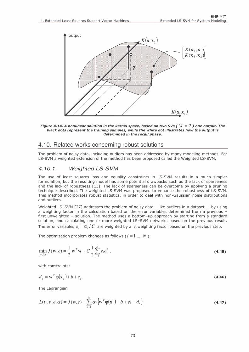
4. Extended Least Squares Support Vector Machines BME-MIT
Extended LS-SVM for System Modeling
73
Figure 4.14. A nonlinear solution in the kernel space, based on two SVs ( 2=M ) one output. The
black dots represent the training samples, while the white dot illustrates how the output is
determined in the recall phase.
4.10. Related works concerning robust solutions
The problem of noisy data, including outliers has been addressed by many modeling methods. For LS-SVM a weighted extension of the method has been proposed called the Weighted LS-SVM.
4.10.1. Weighted LS-SVM
The use of least squares loss and equality constraints in LS-SVM results in a much simpler formulation, but the resulting model has some potential drawbacks such as the lack of sparseness and the lack of robustness [13]. The lack of sparseness can be overcome by applying a pruning technique described. The weighted LS-SVM was proposed to enhance the robustness of LS-SVM. This method incorporates robust statistics, in order to deal with non-Gaussian noise distributions and outliers.
Weighted LS–SVM [27] addresses the problem of noisy data – like outliers in a dataset –, by using a weighting factor in the calculation based on the error variables determined from a previous – first unweighted – solution. The method uses a bottom–up approach by starting from a standard solution, and calculating one or more weighted LS–SVM networks based on the previous result.
The error variables Ce ii /α= are weighted by a iv weighting factor based on the previous step.
The optimization problem changes as follows ( Ni ,...,1= ):
∑=
+=N
i
iiT
ebevCeJ
1
2
,, 2
1
2
1),(min www
w. (4.45)
with constraints:
( ) ii
T
i ebd ++= xw ϕϕϕϕ . (4.46)
The Lagrangian
( ) ∑=
−++−=N
i
iiiT
i debewJebwL1
),();,,( xw ϕϕϕϕαα (4.47)
?
( )1, xxK
( )2,xxKoutput
),(
),(
24
14
xx
xx
K
K
4. Extended Least Squares Support Vector Machines BME-MIT
Extended LS-SVM for System Modeling
74
leads to the following equation set:
=
+ dαΩ1
1T 00 b
VC
r
r
. (4.48)
where
=
Ni
CCvCvCv
diagV1
;...;1
;...;1
1
. (4.49)
The values of the weights iv are determined according to the resulting ie -s (or Ci /α ) of the
previous (first unweighted) solution as follows:
≤≤−
−
≤
=
− otherwise
cseccc
sec
cse
v k
k
k
k
if10
ˆ/ifˆ/
ˆ/if1
4
21
12
2
1
(4.50)
where s is a robust estimate of the standard deviation of the ie error variables:
6745.02ˆ
×=
IQRs . (4.51)
As defined earlier (in section 10.1.2), the interquartile range (IQR) is the difference between the third and first quartiles and is a stable measure of statistical dispersion. The value s gives a measure describing the deviation of the estimated error distribution from a Gaussian distribution. The squared cost function of the unweighted LS-SVM is optimal if the ie error is of Gaussian distribution. For other cases, the described weighting is designed such that the results improve in view of robust statistics. Large ie –s mean small weights and vice versa. The small weight
corresponds to a stronger regularization at the sample. The constants 1c and 2c are usually set to
5,21 =c and 32 =c , which follow from the properties of the Gaussian distribution [13]. The 1c
and 2c can also be determined from the density estimation of the error ( ie ) distribution.
The weighted LS-SVM algorithm:
1. Train an unweighted LS-SVM and compute the Ce ii / α= error values from the solution.
2. Compute a robust estimate of the standard deviation s based on the empirical ie distribution.
3. Calculate the weights iv from ie and s according to (4.51).
4. Solve a new Weighted LS-SVM using the iv values in (4.50).
This algorithm results in a robust solution, through iteratively reducing the effect of samples with the largest error compared to actual estimation.
4.11. Remarks on robust solutions
There are several methods in statistics aiming at noise reduction and outlier detection that can also be used. On the other hand, the propositions presented here for robustness are integrated within the solution method, whilst they use the prior information following also from the method, namely that the solution is linear in the kernel space. This way the

4. Extended Least Squares Support Vector Machines BME-MIT
Extended LS-SVM for System Modeling
75
modeling method itself is extended to pose a robust solution, without requiring any additional analysis of the data
The weighted solutions presented in this section correspond to using a special regularization, where the regularization term is adjusted according to the quality of the sample. This is exactly the same as the original weighted LS-SVM (see section 4.10.1) where the weighted solution of the linear equation set is derived from the idea of using noise sensitive regularization. The other methods proposed from robust statistics do the same thing, but in this case the weighting (or the context sensitive regularization) is determined through a –mostly iterative- method.
According to the propositions, weighting and regularization is closely related to each other. Along with using the least-squares solution to the partially reduced equation set, the regularization term is omitted, but according to this discussion it is introduced through the solution method used – or more specifically through the weighting it determines. This means, that the overdetermined system enables us to use methods that incorporate an “automatic” regularization based on the statistical properties of the training samples.
Just as pruning, this robust method is an iterative process, where every step is based on the result of an LS-SVM solution. This means that the entire large problem must be solved at least once, and a relatively large one in every further iteration step. Another drawback is that pruning and weighting cannot be easily combined, because the methods favor contradictory types of points. While pruning drops the training points belonging to small
iα -s, the weighted LS–SVM increases the effects of these points.

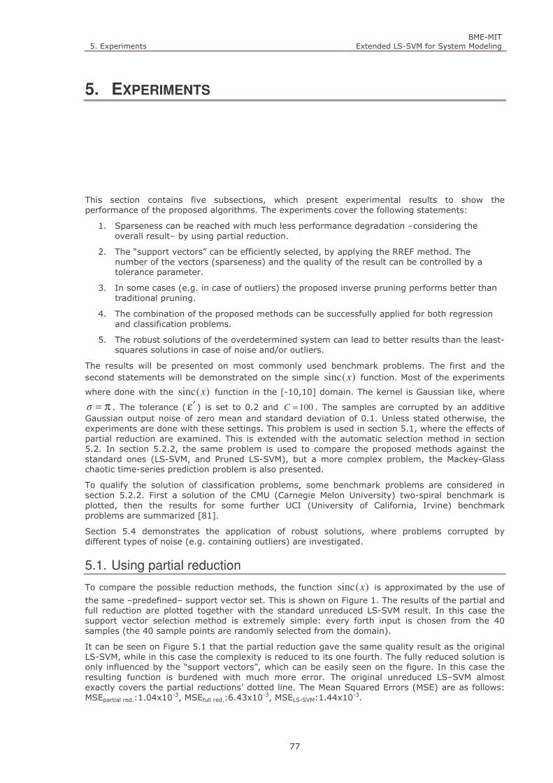
5. Experiments BME-MIT
Extended LS-SVM for System Modeling
77
5. EXPERIMENTS
This section contains five subsections, which present experimental results to show the performance of the proposed algorithms. The experiments cover the following statements:
1. Sparseness can be reached with much less performance degradation –considering the overall result– by using partial reduction.
2. The “support vectors” can be efficiently selected, by applying the RREF method. The number of the vectors (sparseness) and the quality of the result can be controlled by a tolerance parameter.
3. In some cases (e.g. in case of outliers) the proposed inverse pruning performs better than traditional pruning.
4. The combination of the proposed methods can be successfully applied for both regression and classification problems.
5. The robust solutions of the overdetermined system can lead to better results than the least-squares solutions in case of noise and/or outliers.
The results will be presented on most commonly used benchmark problems. The first and the second statements will be demonstrated on the simple )(sinc x function. Most of the experiments
where done with the )(sinc x function in the [-10,10] domain. The kernel is Gaussian like, where
π=σ . The tolerance (ε′ ) is set to 0.2 and 100=C . The samples are corrupted by an additive Gaussian output noise of zero mean and standard deviation of 0.1. Unless stated otherwise, the experiments are done with these settings. This problem is used in section 5.1, where the effects of partial reduction are examined. This is extended with the automatic selection method in section 5.2. In section 5.2.2, the same problem is used to compare the proposed methods against the standard ones (LS-SVM, and Pruned LS-SVM), but a more complex problem, the Mackey-Glass chaotic time-series prediction problem is also presented.
To qualify the solution of classification problems, some benchmark problems are considered in section 5.2.2. First a solution of the CMU (Carnegie Melon University) two-spiral benchmark is plotted, then the results for some further UCI (University of California, Irvine) benchmark problems are summarized [81].
Section 5.4 demonstrates the application of robust solutions, where problems corrupted by different types of noise (e.g. containing outliers) are investigated.
5.1. Using partial reduction
To compare the possible reduction methods, the function )(sinc x is approximated by the use of
the same –predefined– support vector set. This is shown on Figure 1. The results of the partial and full reduction are plotted together with the standard unreduced LS-SVM result. In this case the support vector selection method is extremely simple: every forth input is chosen from the 40 samples (the 40 sample points are randomly selected from the domain).
It can be seen on Figure 5.1 that the partial reduction gave the same quality result as the original LS-SVM, while in this case the complexity is reduced to its one fourth. The fully reduced solution is only influenced by the “support vectors”, which can be easily seen on the figure. In this case the resulting function is burdened with much more error. The original unreduced LS–SVM almost exactly covers the partial reductions’ dotted line. The Mean Squared Errors (MSE) are as follows: MSEpartial red.:1.04x10
-3, MSEfull red.:6.43x10⁻³, MSELS-SVM:1.44x10
-3.

5. Experiments BME-MIT
Extended LS-SVM for System Modeling
78
Figure 5.1. The different reduction methods plotted together.
5.2. Selection Methods
This section summarizes the experiments concerning the proposed selection methods.
5.2.1. The automatic (RREF) selection method
The “support vectors” may be selected automatically, by the use of the RREF selection method.
Figure 5.2. A partially reduced LS–SVM, where the support vectors were selected by the proposed
method (tolerance= 0.2).
-10 -8 -6 -4 -2 0 2 4 6 8 10-0.4
-0.2
0
0.2
0.4
0.6
0.8
1
1.2
input data points
support vectors
partial reduction
-10 -8 -6 -4 -2 0 2 4 6 8 10-0.4
-0.2
0
0.2
0.4
0.6
0.8
1
1.2
1.4
input data points
support vectors
partial reduction
full reduction LS-SVM

5. Experiments BME-MIT
Extended LS-SVM for System Modeling
79
Figure 5.2 shows, a solution that is based on the automatically selected support vector set. Since 40 samples were provided, the original network would have 40 nonlinear kernels, while the reduced net incorporates only 9.
Figure 5.3. The RREF method distributes the kernel centers correctly, even if the data samples are
not distributed evenly (tolerance= 0.001).
Figure 5.3 shows an example to illustrate, how the proposed RREF method distributes the support vectors evenly. The )(sinc x problem is described by 44 data samples, but these are artificially
distributed by selecting 4 points from 11 -evenly placed- small regions. It can be seen, that the RREF method positions the support vectors in the groups, in order to represent each region of the function. This simulation confirms that by omitting the columns that are “nearly” linearly dependent, the RREF method really focuses on creating a sparse representation of the whole problem (equation set).
An even more appealing property of the proposed solution is that the cardinality of the support vector set is indeed independent from the number of training samples. If the problem can be solved with N kernels, then no matter how many inputs are presented, the network size should not change. Table 5.1 shows the number of “support vectors” calculated by the algorithm for different training set sizes of exactly the same problem ( )(sinc x with matching noise etc.
parameters). The mean square errors tested for 100 noise-free samples are also shown. It can be seen that by increasing the number of training samples, the error decreases –as expected–, but the network size does not change significantly.
Table 5.1. The number of support vectors, and the mean squared error (MSE) calculated for
different training set sizes of the same problem using the proposed methods (the tolerance was set
to 0.25).
NUMBER OF TRAINING SAMPLES
(THIS WOULD ALSO BE THE NETWORK
SIZE FOR STANDARD LS-SVM)
NUMBER OF SUPPORT VECTORS
(NETWORK SIZE USING THE RREF METHOD)
MSELS2-SVM
40 8 1.890×10⁻³
80 9 0.877×10⁻³
800 9 0.155×10⁻³
1600 9 0.029×10⁻³
-10 -8 -6 -4 -2 0 2 4 6 8 10-0.4
-0.2
0
0.2
0.4
0.6
0.8
1
1.2
data
SV
LS-LS-SVM
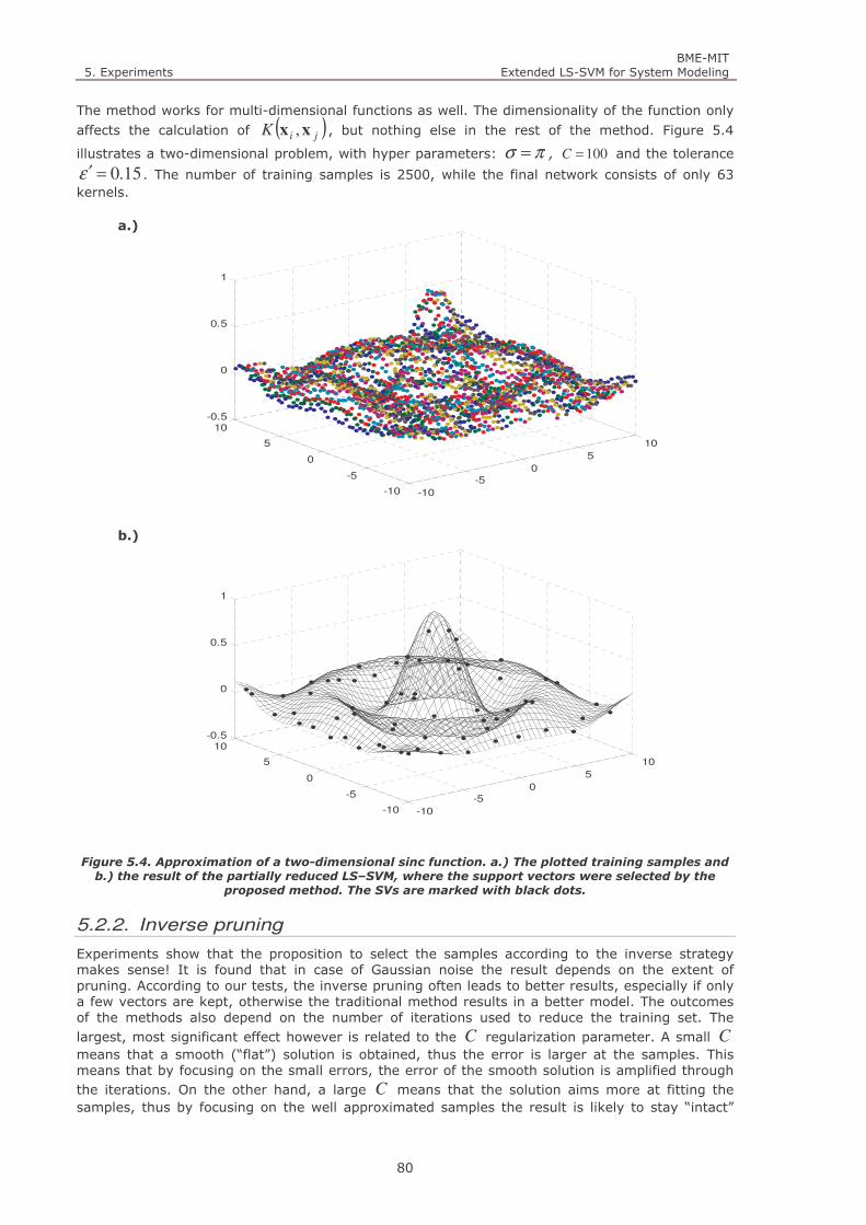
5. Experiments BME-MIT
Extended LS-SVM for System Modeling
80
The method works for multi-dimensional functions as well. The dimensionality of the function only
affects the calculation of ( )jiK xx , , but nothing else in the rest of the method. Figure 5.4
illustrates a two-dimensional problem, with hyper parameters: πσ = , 100=C and the tolerance
15.0=′ε . The number of training samples is 2500, while the final network consists of only 63 kernels.
a.)
b.)
Figure 5.4. Approximation of a two-dimensional sinc function. a.) The plotted training samples and
b.) the result of the partially reduced LS–SVM, where the support vectors were selected by the
proposed method. The SVs are marked with black dots.
5.2.2. Inverse pruning
Experiments show that the proposition to select the samples according to the inverse strategy makes sense! It is found that in case of Gaussian noise the result depends on the extent of pruning. According to our tests, the inverse pruning often leads to better results, especially if only a few vectors are kept, otherwise the traditional method results in a better model. The outcomes of the methods also depend on the number of iterations used to reduce the training set. The largest, most significant effect however is related to the C regularization parameter. A small C means that a smooth (“flat”) solution is obtained, thus the error is larger at the samples. This means that by focusing on the small errors, the error of the smooth solution is amplified through the iterations. On the other hand, a large C means that the solution aims more at fitting the samples, thus by focusing on the well approximated samples the result is likely to stay “intact”
-10
-5
0
5
10
-10
-5
0
5
10-0.5
0
0.5
1
-10
-5
0
5
10
-10
-5
0
5
10-0.5
0
0.5
1

5. Experiments BME-MIT
Extended LS-SVM for System Modeling
81
after reduction. This means that inverse pruning provides better performance in case of good quality (not very noisy) samples, when a large C should be used. The problem is exactly the same from the viewpoint of the traditional pruning. In case of a large regularization, the model tries to fit the samples as accurately as it can. By keeping the erroneous samples, the error of the approximation is amplified. Figure 5.5 box plots the MSE distributions and illustrates the results by showing the result of one experiment.
a.) C=10
b.) C=100
c.) C=100000
normal pr. inverse pr.
0
0.05
0.1
0.15
0.2
Valu
es
-15 -10 -5 0 5 10 15-0.5
0
0.5
1
1.5
sinc
normal pr.
normal sampl.
inverse pr.
inverse sampl.
normal pr. inverse pr.
0
0.05
0.1
0.15
0.2
0.25
Valu
es
-15 -10 -5 0 5 10 15-0.5
0
0.5
1
1.5
sinc
normal pr.
normal sampl.
inverse pr.
inverse sampl.
normal pr. inverse pr.
0
0.1
0.2
0.3
0.4
Valu
es
-15 -10 -5 0 5 10 15-0.5
0
0.5
1
1.5
sinc
normal pr.
normal sampl.
inverse pr.
inverse sampl.
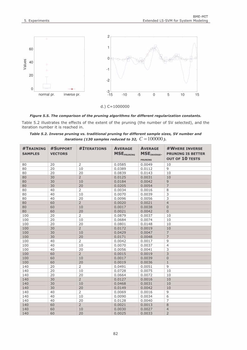
5. Experiments BME-MIT
Extended LS-SVM for System Modeling
82
d.) C=1000000
Figure 5.5. The comparison of the pruning algorithms for different regularization constants.
Table 5.2 illustrates the effects of the extent of the pruning (the number of SV selected), and the iteration number it is reached in.
Table 5.2. Inverse pruning vs. traditional pruning for different sample sizes, SV number and
iterations (130 samples reduced to 32, 100000=C ).
#TRAINING SAMPLES
#SUPPORT VECTORS
#ITERATIONS AVERAGE MSEPRUNING
AVERAGE MSEINVERSE-
PRUNING
#WHERE INVERSE
PRUNING IS BETTER
OUT OF 10 TESTS
80 20 2 0.0585 0.0049 10 80 20 10 0.0389 0.0112 9 80 20 20 0.0839 0.0143 10 80 30 2 0.0125 0.0031 10 80 30 10 0.0184 0.0042 9 80 30 20 0.0205 0.0054 7 80 40 2 0.0034 0.0016 8 80 40 10 0.0070 0.0039 3 80 40 20 0.0096 0.0056 3 80 60 2 0.0020 0.0021 4 80 60 10 0.0017 0.0038 0 80 60 20 0.0021 0.0042 0 100 20 2 0.0879 0.0037 10 100 20 10 0.0684 0.0074 10 100 20 20 0.0801 0.0148 10 100 30 2 0.0172 0.0019 10 100 30 10 0.0429 0.0047 7 100 30 20 0.0171 0.0048 7 100 40 2 0.0042 0.0017 9 100 40 10 0.0070 0.0037 4 100 40 20 0.0056 0.0041 3 100 60 2 0.0015 0.0019 3 100 60 10 0.0017 0.0039 0 100 60 20 0.0019 0.0036 1 140 20 2 0.0491 0.0051 9 140 20 10 0.0728 0.0075 10 140 20 20 0.0664 0.0072 10 140 30 2 0.0127 0.0016 10 140 30 10 0.0468 0.0031 10 140 30 20 0.0149 0.0042 10 140 40 2 0.0069 0.0016 9 140 40 10 0.0090 0.0034 6 140 40 20 0.0128 0.0040 7 140 60 2 0.0021 0.0013 8 140 60 10 0.0030 0.0027 4 140 60 20 0.0025 0.0033 2
normal pr. inverse pr.
0
20
40
60
Valu
es
-15 -10 -5 0 5 10 15-3
-2
-1
0
1
2
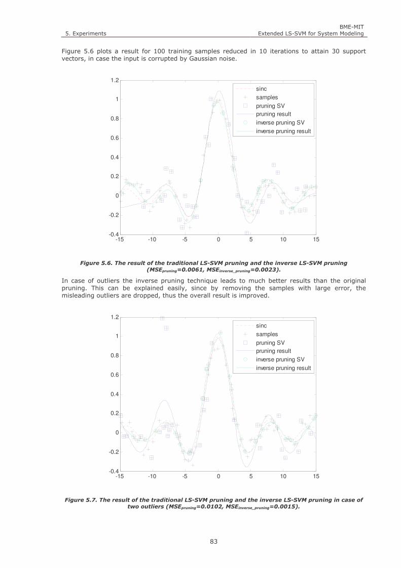
5. Experiments BME-MIT
Extended LS-SVM for System Modeling
83
Figure 5.6 plots a result for 100 training samples reduced in 10 iterations to attain 30 support vectors, in case the input is corrupted by Gaussian noise.
Figure 5.6. The result of the traditional LS-SVM pruning and the inverse LS-SVM pruning
(MSEpruning=0.0061, MSEinverse_pruning=0.0023).
In case of outliers the inverse pruning technique leads to much better results than the original pruning. This can be explained easily, since by removing the samples with large error, the misleading outliers are dropped, thus the overall result is improved.
Figure 5.7. The result of the traditional LS-SVM pruning and the inverse LS-SVM pruning in case of
two outliers (MSEpruning=0.0102, MSEinverse_pruning=0.0015).
-15 -10 -5 0 5 10 15-0.4
-0.2
0
0.2
0.4
0.6
0.8
1
1.2
sinc
samples
pruning SV
pruning result
inverse pruning SV
inverse pruning result
-15 -10 -5 0 5 10 15-0.4
-0.2
0
0.2
0.4
0.6
0.8
1
1.2
sinc
samples
pruning SV
pruning result
inverse pruning SV
inverse pruning result

5. Experiments BME-MIT
Extended LS-SVM for System Modeling
84
It must also be noted, that the inverse pruning technique eliminates the contradiction between traditional pruning and weighting methods described in the last remark of section 4.11. The problem originates in that traditional LS-SVM pruning removes the samples with small error, the ones that the weighting method would favor. If inverse pruning is applied the two methods are “synchronized”, since the pruning omits the points that the weighting would suppress (reducing its influence, by allowing large error at this point). Figure 5.7 shows a result calculated in case of two outliers. The experimental setup is the same as in the previous illustration.
5.2.3. Comparison of selection methods
To evaluate the reduction methods (summarized in section 4.7) several experiments have been done. Due to the infinite number of possible problems and the large number of parameters, it is very hard to construct a representative experiment.
First a noisy )sinc(x is approximated based on 120=N , with parameters πσ = , 100=C ,
01.0=′ε (RREF tolerance) which concludes to 19 support vectors. The number of support vectors is determined by the RREF method (using the given tolerance), and all other methods are configured to achieve the same size. The results are potted in the following box plot, where the MSE of 30 different sampling –the difference is due to the random sampling and error- is plotted for each selection method.
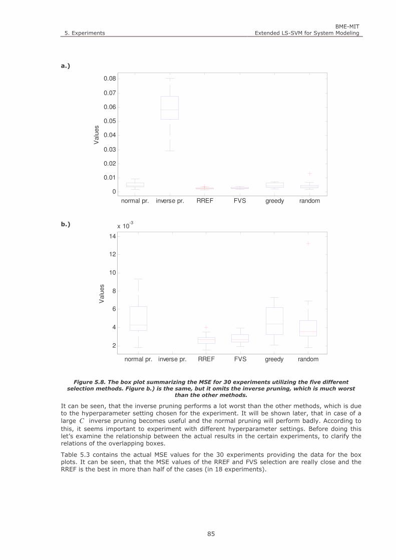
5. Experiments BME-MIT
Extended LS-SVM for System Modeling
85
a.)
b.)
Figure 5.8. The box plot summarizing the MSE for 30 experiments utilizing the five different
selection methods. Figure b.) is the same, but it omits the inverse pruning, which is much worst
than the other methods.
It can be seen, that the inverse pruning performs a lot worst than the other methods, which is due to the hyperparameter setting chosen for the experiment. It will be shown later, that in case of a large C inverse pruning becomes useful and the normal pruning will perform badly. According to this, it seems important to experiment with different hyperparameter settings. Before doing this let’s examine the relationship between the actual results in the certain experiments, to clarify the relations of the overlapping boxes.
Table 5.3 contains the actual MSE values for the 30 experiments providing the data for the box plots. It can be seen, that the MSE values of the RREF and FVS selection are really close and the RREF is the best in more than half of the cases (in 18 experiments).
normal pr. inverse pr. RREF FVS greedy random
0
0.01
0.02
0.03
0.04
0.05
0.06
0.07
0.08
Valu
es
normal pr. inverse pr. RREF FVS greedy random
2
4
6
8
10
12
14
x 10-3
Valu
es
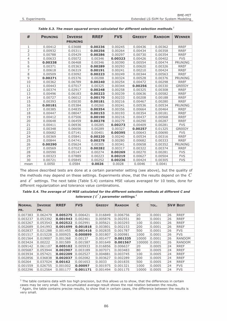
5. Experiments BME-MIT
Extended LS-SVM for System Modeling
86
Table 5.3. The mean squared errors calculated for different selection methods.3
# PRUNING INVERSE PRUNING
RREF FVS GREEDY RANDOM WINNER
1 0.00412 0.03688 0.00236 0.00245 0.00436 0.00362 RREF 2 0.00932 0.05311 0.00256 0.00264 0.00434 0.00358 RREF 3 0.00788 0.05429 0.00286 0.00297 0.00730 0.00354 RREF 4 0.00633 0.05072 0.00346 0.00323 0.00426 0.00402 FVS 5 0.00338 0.06468 0.00346 0.00390 0.00554 0.00474 PRUNING 6 0.00371 0.05363 0.00289 0.00293 0.00620 0.00326 RREF 7 0.00618 0.06319 0.00191 0.00241 0.00210 0.00424 RREF 8 0.00509 0.03092 0.00223 0.00249 0.00344 0.00563 RREF 9 0.00271 0.05376 0.00288 0.00324 0.00528 0.00376 PRUNING 10 0.00362 0.06789 0.00240 0.00254 0.00472 0.00298 RREF 11 0.00443 0.07017 0.00325 0.00344 0.00256 0.00330 GREEDY 12 0.00374 0.02917 0.00248 0.00258 0.00325 0.00308 RREF 13 0.00496 0.06183 0.00223 0.00239 0.00636 0.00582 RREF 14 0.00727 0.06012 0.00170 0.00233 0.00208 0.00188 RREF 15 0.00393 0.05030 0.00181 0.00216 0.00467 0.00280 RREF 16 0.00181 0.05384 0.00260 0.00241 0.00536 0.00534 PRUNING 17 0.00385 0.04835 0.00354 0.00356 0.00664 0.00464 RREF 18 0.00447 0.08047 0.00153 0.00193 0.00354 0.00181 RREF 19 0.00412 0.07506 0.00190 0.00216 0.00437 0.00568 RREF 20 0.00648 0.06459 0.00278 0.00279 0.00290 0.00287 RREF 21 0.00411 0.06936 0.00285 0.00273 0.00409 0.00281 FVS 22 0.00348 0.06656 0.00289 0.00327 0.00257 0.01325 GREEDY 23 0.00682 0.07141 0.00401 0.00395 0.00643 0.00690 FVS 24 0.00369 0.05841 0.00220 0.00240 0.00534 0.00316 RREF 25 0.00844 0.04741 0.00278 0.00280 0.00682 0.00333 RREF 26 0.00290 0.05624 0.00305 0.00341 0.00658 0.00352 PRUNING 27 0.00569 0.07023 0.00282 0.00317 0.00322 0.00374 RREF 28 0.00590 0.05147 0.00274 0.00269 0.00270 0.00281 FVS 29 0.00323 0.07889 0.00223 0.00219 0.00627 0.00504 FVS 30 0.00721 0.05845 0.00252 0.00236 0.00424 0.00305 FVS
mean 0.0050 0.0584 0.0026 0.0028 0.0046 0.0041
The above described tests are done at a certain parameter setting (see above), but the quality of the methods may depend on these settings. Experiments show, that the results depend on the C
and ε ′ settings. The next table (Table 5.4) contains MSE values averaged for 10 tests, done for different regularization and tolerance value combinations.
Table 5.4. The average of 10 MSE calculated for the different selection methods at different C and
tolerance (ε ′ ) parameter settings.4
NORMAL
PR.
INVERSE
PR.
RREF FVS GREEDY RANDOM C TOL. SV# BEST
0.007383 0.062479 0.005275 0.006421 0.016849 0.006756 20 0.0001 26 RREF 0.003237 0.053392 0.001943 0.002461 0.005876 0.002551 80 0.0001 26 RREF 0.003267 0.053543 0.002522 0.002991 0.005621 0.003293 100 0.0001 26 RREF 0.002689 0.041993 0.001699 0.001818 0.003801 0.002153 200 0.0001 26 RREF 0.002837 0.021288 0.001455 0.001416 0.002835 0.001787 500 0.0001 26 FVS 0.001517 0.015228 0.000925 0.000899 0.001807 0.000981 1000 0.0001 26 FVS 0.001564 0.019007 0.001368 0.00137 0.001477 0.001335 10000 0.0001 26 RANDOM 0.003424 0.00222 0.001589 0.001587 0.001649 0.001567 100000 0.0001 26 RANDOM 0.009142 0.061107 0.005102 0.005933 0.016856 0.006637 20 0.0005 24 RREF 0.005687 0.053944 0.002907 0.003189 0.007071 0.003483 80 0.0005 24 RREF 0.003934 0.057421 0.002209 0.002527 0.004881 0.003745 100 0.0005 24 RREF 0.002856 0.036838 0.002037 0.002082 0.003627 0.002289 200 0.0005 24 RREF 0.00264 0.037024 0.00162 0.001653 0.0033 0.001835 500 0.0005 24 RREF 0.001559 0.026755 0.001002 0.00097 0.001975 0.001321 1000 0.0005 24 FVS 0.002296 0.012564 0.001177 0.001171 0.001494 0.001175 10000 0.0005 24 FVS
3 The table contains data with too high precision, but this allows us to show, that the differences in certain cases may be very small. The accumulated average result shows the real relation between the results. 4 Again, the table contains precise results, to show that in certain cases, the difference between the results is very small.
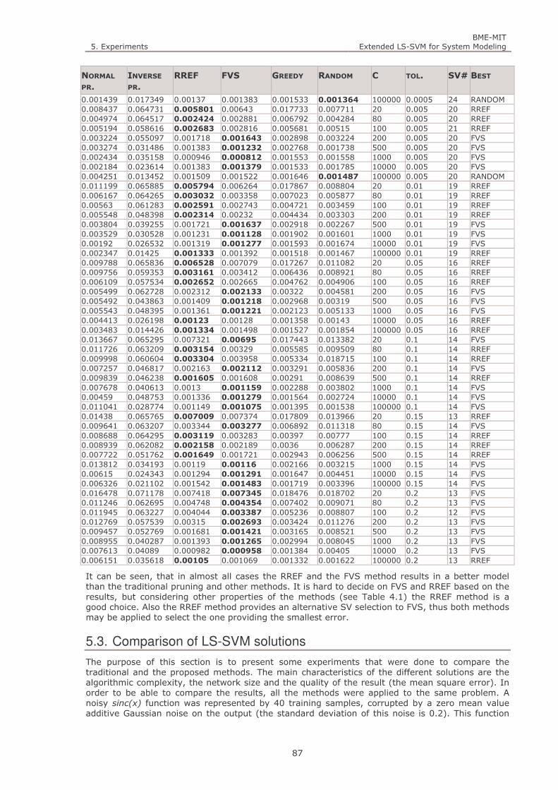
5. Experiments BME-MIT
Extended LS-SVM for System Modeling
87
NORMAL
PR.
INVERSE
PR.
RREF FVS GREEDY RANDOM C TOL. SV# BEST
0.001439 0.017349 0.00137 0.001383 0.001533 0.001364 100000 0.0005 24 RANDOM 0.008437 0.064731 0.005801 0.00643 0.017733 0.007711 20 0.005 20 RREF 0.004974 0.064517 0.002424 0.002881 0.006792 0.004284 80 0.005 20 RREF 0.005194 0.058616 0.002683 0.002816 0.005681 0.00515 100 0.005 21 RREF 0.003224 0.055097 0.001718 0.001643 0.002898 0.003224 200 0.005 20 FVS 0.003274 0.031486 0.001383 0.001232 0.002768 0.001738 500 0.005 20 FVS 0.002434 0.035158 0.000946 0.000812 0.001553 0.001558 1000 0.005 20 FVS 0.002184 0.023614 0.001383 0.001379 0.001533 0.001785 10000 0.005 20 FVS 0.004251 0.013452 0.001509 0.001522 0.001646 0.001487 100000 0.005 20 RANDOM 0.011199 0.065885 0.005794 0.006264 0.017867 0.008804 20 0.01 19 RREF 0.006167 0.064265 0.003032 0.003358 0.007023 0.005877 80 0.01 19 RREF 0.00563 0.061283 0.002591 0.002743 0.004721 0.003459 100 0.01 19 RREF 0.005548 0.048398 0.002314 0.00232 0.004434 0.003303 200 0.01 19 RREF 0.003804 0.039255 0.001721 0.001637 0.002918 0.002267 500 0.01 19 FVS 0.003529 0.030528 0.001231 0.001128 0.001902 0.001601 1000 0.01 19 FVS 0.00192 0.026532 0.001319 0.001277 0.001593 0.001674 10000 0.01 19 FVS 0.002347 0.01425 0.001333 0.001392 0.001518 0.001467 100000 0.01 19 RREF 0.009788 0.065836 0.006528 0.007079 0.017267 0.011082 20 0.05 16 RREF 0.009756 0.059353 0.003161 0.003412 0.006436 0.008921 80 0.05 16 RREF 0.006109 0.057534 0.002652 0.002665 0.004762 0.004906 100 0.05 16 RREF 0.005499 0.062728 0.002312 0.002133 0.00322 0.004581 200 0.05 16 FVS 0.005492 0.043863 0.001409 0.001218 0.002968 0.00319 500 0.05 16 FVS 0.005543 0.048395 0.001361 0.001221 0.002123 0.005133 1000 0.05 16 FVS 0.004413 0.026198 0.00123 0.00128 0.001358 0.00143 10000 0.05 16 RREF 0.003483 0.014426 0.001334 0.001498 0.001527 0.001854 100000 0.05 16 RREF 0.013667 0.065295 0.007321 0.00695 0.017443 0.013382 20 0.1 14 FVS 0.011726 0.063209 0.003154 0.00329 0.005585 0.009509 80 0.1 14 RREF 0.009998 0.060604 0.003304 0.003958 0.005334 0.018715 100 0.1 14 RREF 0.007257 0.046817 0.002163 0.002112 0.003291 0.005836 200 0.1 14 FVS 0.009839 0.046238 0.001605 0.001608 0.00291 0.008639 500 0.1 14 RREF 0.007678 0.040613 0.0013 0.001159 0.002288 0.003802 1000 0.1 14 FVS 0.00459 0.048753 0.001336 0.001279 0.001564 0.002724 10000 0.1 14 FVS 0.011041 0.028774 0.001149 0.001075 0.001395 0.001538 100000 0.1 14 FVS 0.01438 0.065765 0.007009 0.007374 0.017809 0.013966 20 0.15 13 RREF 0.009641 0.063207 0.003344 0.003277 0.006892 0.011318 80 0.15 14 FVS 0.008688 0.064295 0.003119 0.003283 0.00397 0.00777 100 0.15 14 RREF 0.008939 0.062082 0.002158 0.002189 0.0036 0.006287 200 0.15 14 RREF 0.007722 0.051762 0.001649 0.001721 0.002943 0.006256 500 0.15 14 RREF 0.013812 0.034193 0.00119 0.00116 0.002166 0.003215 1000 0.15 14 FVS 0.00615 0.024343 0.001294 0.001291 0.001647 0.004451 10000 0.15 14 FVS 0.006326 0.021102 0.001542 0.001483 0.001719 0.003396 100000 0.15 14 FVS 0.016478 0.071178 0.007418 0.007345 0.018476 0.018702 20 0.2 13 FVS 0.011246 0.062695 0.004748 0.004354 0.007402 0.009071 80 0.2 13 FVS 0.011945 0.063227 0.004044 0.003387 0.005236 0.008807 100 0.2 12 FVS 0.012769 0.057539 0.00315 0.002693 0.003424 0.011276 200 0.2 13 FVS 0.009457 0.052769 0.001681 0.001421 0.003165 0.008521 500 0.2 13 FVS 0.008955 0.040287 0.001393 0.001265 0.002994 0.008045 1000 0.2 13 FVS 0.007613 0.04089 0.000982 0.000958 0.001384 0.00405 10000 0.2 13 FVS 0.006151 0.035618 0.00105 0.001069 0.001332 0.001622 100000 0.2 13 RREF
It can be seen, that in almost all cases the RREF and the FVS method results in a better model than the traditional pruning and other methods. It is hard to decide on FVS and RREF based on the results, but considering other properties of the methods (see Table 4.1) the RREF method is a good choice. Also the RREF method provides an alternative SV selection to FVS, thus both methods may be applied to select the one providing the smallest error.
5.3. Comparison of LS-SVM solutions
The purpose of this section is to present some experiments that were done to compare the traditional and the proposed methods. The main characteristics of the different solutions are the algorithmic complexity, the network size and the quality of the result (the mean square error). In order to be able to compare the results, all the methods were applied to the same problem. A noisy sinc(x) function was represented by 40 training samples, corrupted by a zero mean value additive Gaussian noise on the output (the standard deviation of this noise is 0.2). This function
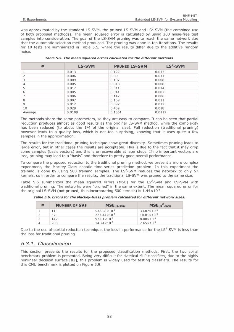
5. Experiments BME-MIT
Extended LS-SVM for System Modeling
88
was approximated by the standard LS-SVM, the pruned LS-SVM and LS2-SVM (the combined use of both proposed methods). The mean squared error is calculated by using 200 noise-free test samples into consideration. The goal of the LS-SVM pruning was to reach the same network size that the automatic selection method produced. The pruning was done in ten iterations. The results for 10 tests are summarized in Table 5.5, where the results differ due to the additive random noise.
Table 5.5. The mean squared errors calculated for the different methods.
# LS-SVM PRUNED LS-SVM LS2-SVM
1 0.013 0.122 0.017 2 0.006 0.09 0.011 3 0.009 0.107 0.008 4 0.005 0.018 0.008 5 0.017 0.311 0.014 6 0.005 0.041 0.007 7 0.006 0.147 0.006 8 0.007 0.169 0.011 9 0.012 0.097 0.012 10 0.029 0.459 0.018 Average 0.0109 0.1561 0.0112
The methods share the same parameters, so they are easy to compare. It can be seen that partial reduction produces almost as good results as the original LS-SVM method, while the complexity has been reduced (to about the 1/4 of the original size). Full reduction (traditional pruning) however leads to a quality loss, which is not too surprising, knowing that it uses quite a few samples in the approximation.
The results for the traditional pruning technique show great diversity. Sometimes pruning leads to large error, but in other cases the results are acceptable. This is due to the fact that it may drop some samples (basis vectors) and this is unrecoverable at later steps. If no important vectors are lost, pruning may lead to a “basis” and therefore to pretty good overall performance.
To compare the proposed reduction to the traditional pruning method, we present a more complex experiment, the Mackey-Glass chaotic time-series prediction problem. In this experiment the training is done by using 500 training samples. The LS2-SVM reduces the network to only 57 kernels, so in order to compare the results, the traditional LS-SVM was pruned to the same size.
Table 5.6 summarizes the mean squared errors (MSE) for the LS2-SVM and LS-SVM with traditional pruning. The networks were “pruned” in the same extent. The mean squared error for the original LS-SVM (not pruned, thus incorporating 500 kernels) is 1.44×10⁻⁵.
Table 5.6. Errors for the Mackey-Glass problem calculated for different network sizes.
# NUMBER OF SVS MSELS-SVM MSELS2-SVM
1 11 532.58×10⁻⁵ 33.07×10⁻⁵ 2 57 223.44×10⁻⁵ 10.81×10⁻⁵ 3 142 97.01×10⁻⁵ 8.08×10⁻⁵ 4 208 14.74×10⁻⁵ 7.65×10⁻⁵
Due to the use of partial reduction technique, the loss in performance for the LS2-SVM is less than the loss for traditional pruning.
5.3.1. Classification
This section presents the results for the proposed classification methods. First, the two spiral benchmark problem is presented. Being very difficult for classical MLP classifiers, due to the highly nonlinear decision surface [82], this problem is widely used for testing classifiers. The results for this CMU benchmark is plotted on Figure 5.9.

5. Experiments BME-MIT
Extended LS-SVM for System Modeling
89
a.) b.)
Figure 5.9. The classification boundaries obtained for the standard LS–SVM a.) and the LS2–SVM
b.).
Both LS-SVM and LS2-SVM obtains zero error on the training samples and good generalization properties. The traditional method uses all 194 samples, while the proposed least squares solution solves this problem with only 137 support vectors. If the tolerance is chosen to be larger, then the complexity may be even further reduced, but in that case the generalization ability degrades.
Table 5.7 summarizes the results for some UCI benchmarks. The results described here may not be the ones achieved for optimal hyper–parameter settings, but it is not that important in the comparison of LS-SVM (no pruning is applied) and LS2-SVM, especially in the light of their equivalence if 0 tolerance is used. Of course, in the experiments we were aiming at using nearly optimal hyper parameter settings. The datasets were split to train and test sets as seen in Table 5.7 which corresponds to the experiments of ref. [13].
Table 5.7. Results achieved for benchmark problems. Where NTR is the number of training inputs
and NTS is the number of test samples. The NLS-SVM and NLS2-SVM columns contain the network size of
the solutions respectively. The hit/miss classification rates are also shown for both methods the
test sets.
BENCHMARK NTR NTST NLS-SVM LS-SVM NLS2-SVM LS2-SVM
HIT% MISS% HIT% MISS%
Bupa liver
disorders
230 115 230 67.82 32.18 37 70.44 29.56
Pima Indians
diabetes
512 256 512 67.97 32.03 379 68.36 31.64
Tic–tac–toe
endgame
638 320 638 97.19 2.81 136 94.37 5.63
Statlog heart
disease
180 90 180 72.23 27.77 168 70.00 30.00
It can be seen that for simple problems consisting many samples, the gain is high, since a lot of samples may be pruned (e.g. Bupa liver disorders), while for hard problems, with a small sample set (e.g. Statlog heart disease) the network size cannot be reduced. Sometimes performance may degrade with reduction; therefore the degree of reduction must be determined according to a trade–off between size and performance.
5.3.2. Dynamic problems/Time series prediction
The next figure (Figure 5.10) shows a solution to the widely used Mackey-Glass time series prediction problem. In the prediction we have used the [-6,-12,-18,-24] delays, thus the x(t) value of the t -th time instant is approximated by four past values (in Mackey-Glass process, there is no input – the output only depends on the past values). In this experiment the training is done by using 500 training samples.
-8 -6 -4 -2 0 2 4 6 8-6
-4
-2
0
2
4
6
8
-8 -6 -4 -2 0 2 4 6 8-6
-4
-2
0
2
4
6
8

5. Exp
erim
ents
BME-M
IT
Exten
ded
LS-SVM for System M
odeling
90
a.)
b.)
c.)
Figure 5.10. The predicte
d values and the errors for the M
ackey-Glass prediction problem. a.) The results for the traditional LS–SVM b.) the result of LS–
SVM w
ith traditional pruning c.) the result for the proposed m
eth
ods. The pruned, and the LS
2-SVM results conta
in only 68 support vecto
rs.
0200
400
600
800
1000
1200
0
0.51
1.5
0200
400
600
800
1000
1200
-0.4
-0.20
0.2
0.4
Train data
Test data
0200
400
600
800
1000
1200
0
0.51
1.5
0200
400
600
800
1000
1200
-0.4
-0.20
0.2
0.4
0200
400
600
800
1000
1200
0
0.51
1.5
0200
400
600
800
1000
1200
-0.4
-0.20
0.2
0.4

5. Experiments BME-MIT
Extended LS-SVM for System Modeling
91
This experiment shows that the above/described solution along with LS-SVM regression is applicable to solve time series prediction problems. In the presented solution, the traditional LS–SVM uses 500 neurons, while the LS2–SVM reduces the network to only 68 neurons (the traditional LS-SVM b.) was pruned to the same size).
With a larger tolerance value, we can achieve much smaller networks, but consequently the error of the estimation grows. It is easy to see, that the selection of the ε ′ tolerance is a trade–off problem between network size and performance. Due to the use of partial reduction technique, the loss in performance for the LS2–SVM is less, than the loss for traditional pruning.
The next table (Table 5.8.) summarizes the mean squared errors (MSE) for the LS2–SVM, and LS–SVM with traditional pruning. The networks were “pruned” in the same extent. The mean squared error for the full (not pruned) LS–SVM is 1.44x10⁻⁵.
Table 5.8. Errors for the Mackey-Glass problem calculated for different network sizes.
NUMBER OF NEURONS MSEPRUNED LS-SVM MSELS2-SVM
1 11 532.58x10⁻⁵ 33.07 x10⁻⁵ 2 57 223.44 x10⁻⁵ 10.81 x10⁻⁵ 3 142 97.01 x10⁻⁵ 8.08 x10⁻⁵ 4 208 14.74 x10⁻⁵ 7.65 x10⁻⁵
5.4. Robust methods
The next figure (Figure 5.11) plots the result of the bisquare weights method applied to the same problem.
Figure 5.11. The continuous black line plots the result for a partially reduced LS-SVM solved by the
bisquare weights method. (MSEbisquare-SVM= 1.89*10-3, MSELS-SVM= 6.86*10-2).
The next example (Figure 5.12) presents another robust solution, the least trimmed squares solution (LTS LS-SVM) which completely discards some samples (with the largest error), from the optimization problem.
-10 -8 -6 -4 -2 0 2 4 6 8 10-1.5
-1
-0.5
0
0.5
1
1.5
2
input data points
support vectors
bisquare-SVM
LS-SVM
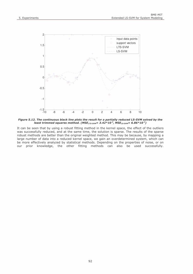
5. Experiments BME-MIT
Extended LS-SVM for System Modeling
92
Figure 5.12. The continuous black line plots the result for a partially reduced LS-SVM solved by the
least trimmed squares method. (MSELTS-SVM= 3.42*10-3, MSELS-SVM= 6.86*10-2)
It can be seen that by using a robust fitting method in the kernel space, the effect of the outliers was successfully reduced, and at the same time, the solution is sparse. The results of the sparse robust methods are better than the original weighted method. This may be because, by mapping a large number of data into a reduced kernel space, we gain an overdetermined system, which can be more effectively analyzed by statistical methods. Depending on the properties of noise, or on our prior knowledge, the other fitting methods can also be used successfully.
-10 -8 -6 -4 -2 0 2 4 6 8 10-1.5
-1
-0.5
0
0.5
1
1.5
2
input data points
support vectors
LTS-SVM
LS-SVM

6. Other LS-SVM extensions BME-MIT
Extended LS-SVM for System Modeling
93
6. OTHER LS-SVM EXTENSIONS
This section contains some further extensions to LS-SVM that do not fit directly into the framework of extended LS-SVM described above:
A heuristic outlier detection method is described.
A generalized LS-SVM formulation is given.
6.1. Outlier detection
This section discusses a noise reduction technique for the case when the training samples contain some outliers (due to some non–Gaussian noise). This solution is based on the fact that once our equation set is overdetermined some ( MN − ) rows (constraints) may be removed and the equation set can still be solved. But which rows should be removed? Let’s define some (M ) vectors as support vectors. Every training sample, input–output pair, defines a constraint, which is represented by an equation. Provided that enough training points are available to learn the function, than the addition of new samples –equations– should not change the solution. This means, that this equation linearly dependent from the others. Our goal is to remove some equations, such that the error of the least–squares solution is minimized. This can be done by using a “linearly dependent” subset of equations and leaving out the most linearly independent ones. Just like in the SV selection method, the linear dependence discussed here, does not mean exact linear dependence, only in a sense of a “resemblance” (parallelism) measure. The removed equations are the ones that are the least resembling to the others.
The selection can be illustrated as follows.
1. Fit an 1+N –dimensional hyperplane on the points defined by the rows of the matrix [ ]dΩ .
2. Calculate the distance of every point from this plane.
3. Leave out the points with the largest distance.
If the number of the kernel functions is M , and the training set has N samples, than at most
MN − equations may be removed, otherwise the equation set will become underdetermined. In most cases it is unnecessary to leave out that many points, since the more constraints are considered; the better results can be expected.
In the next experiment 5 input points are changed to outliers. These outliers are detected by the use of the described noise reduction method. The support vectors are selected from the training samples with the use of the RREF based method. The input points are plotted, where the detected outliers are marked with large dots.

6. Other LS-SVM extensions BME-MIT
Extended LS-SVM for System Modeling
94
Figure 6.1. The grey dashed line is the original LS-SVM’s result, while the continuous black line
plots the result for the proposed method.
It is important to mention that the results are based on a much smaller network (11 neurons) , since the number of columns was also reduced.
6.2. Generalized LS-SVM formulation
The described extended LS-SVM technique shows that the columns and rows may be handled independently, therefore the equation set may be generalized further.
Each column (j) stands for a neuron, with a kernel centered on the corresponding input ( jx ).
However in a generalized case:
The kernels may be centered around any point (not just input samples), so the columns may be represented by any chosen jc vector. For example the most simple construction of
a fixed LS–SVM is to define the centers (e.g. M uniformly positioned vectors in the input space), and solve the equation set (4.21) –or originally (4.6)- formulated accordingly.
The kernel functions may be different form column to column.
The formulation of Ω and the equation set changes as follows:
( )jijji K cx ,, =Ω (6.1)
and the result will be calculated from:
( )∑ =+=
M
i iii bKαy0
,cx , (6.2)
where M is the number of kernels used and iK is the i-th kernel function.
Just as earlier in the partial reduction case, there is a slight problem with the regularization parameter C , since it can only be inserted in the first M rows. This doesn’t exactly reflect the same theoretical meaning as in the original equation (4.6), but it is enough to ensure M linearly independent rows, so the equation set can be solved (see section 4.1).
-20 -15 -10 -5 0 5 10 15 20-3
-2
-1
0
1
2
3
4
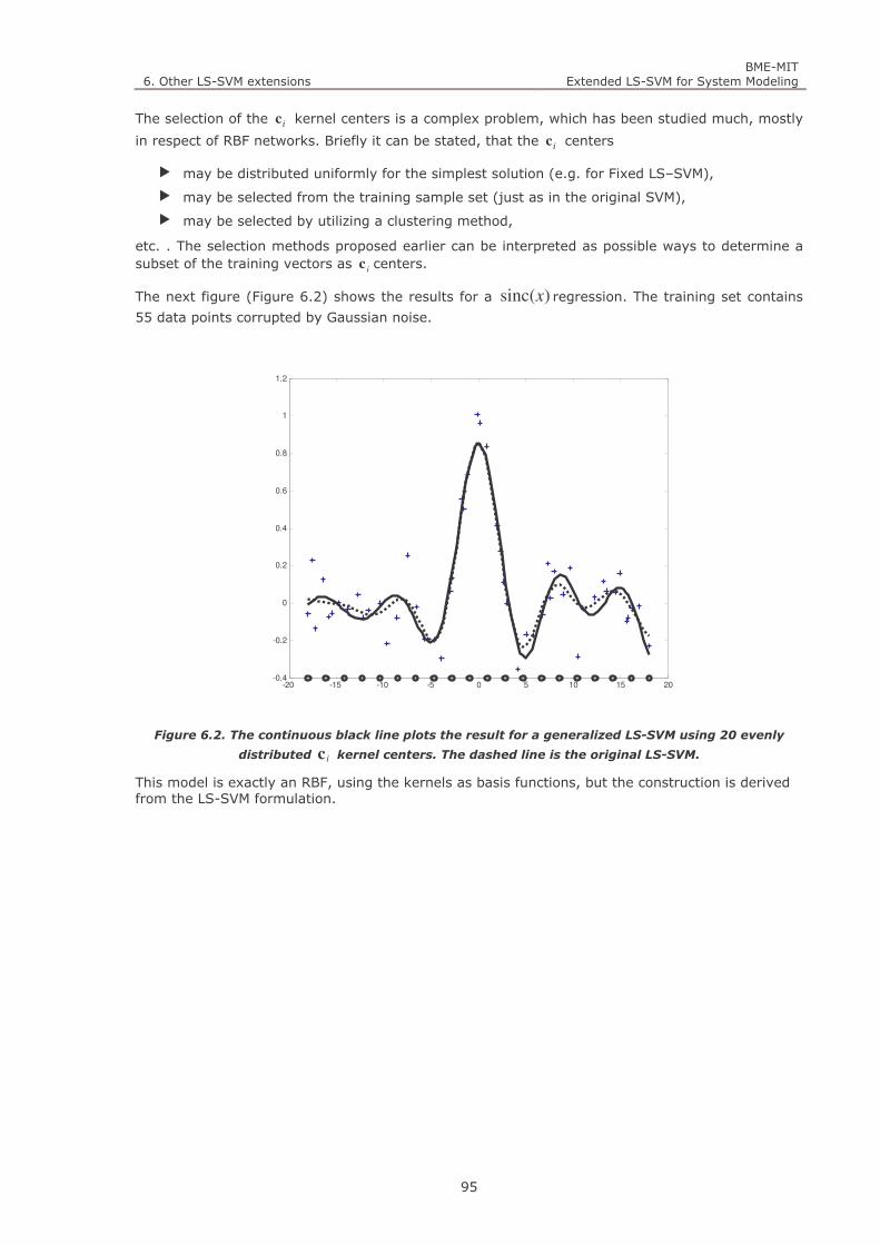
6. Other LS-SVM extensions BME-MIT
Extended LS-SVM for System Modeling
95
The selection of the ic kernel centers is a complex problem, which has been studied much, mostly
in respect of RBF networks. Briefly it can be stated, that the ic centers
may be distributed uniformly for the simplest solution (e.g. for Fixed LS–SVM),
may be selected from the training sample set (just as in the original SVM),
may be selected by utilizing a clustering method,
etc. . The selection methods proposed earlier can be interpreted as possible ways to determine a subset of the training vectors as ic centers.
The next figure (Figure 6.2) shows the results for a )sinc(x regression. The training set contains
55 data points corrupted by Gaussian noise.
Figure 6.2. The continuous black line plots the result for a generalized LS-SVM using 20 evenly
distributed ic kernel centers. The dashed line is the original LS-SVM.
This model is exactly an RBF, using the kernels as basis functions, but the construction is derived from the LS-SVM formulation.
-20 -15 -10 -5 0 5 10 15 20-0.4
-0.2
0
0.2
0.4
0.6
0.8
1
1.2


7. Industrial system modeling – a steelmaking process BME-MIT
Extended LS-SVM for System Modeling
97
7. INDUSTRIAL SYSTEM MODELING – A STEELMAKING
PROCESS
In this section the extended LS-SVM methods are applied to model a real-life industrial process, namely the steelmaking with a Linz-Donawitz converter. This process is believed to be a typical example of complex industrial processes where many parameters are noisy and imprecise due to the harsh industrial environment and the extreme circumstances (Figure 7.1).
Figure 7.1. Photo of an LD steel converter.
7.1. Background
The Linz-Donawitz (LD) converter steelmaking problem was a large project of the Department of Measurement and Information Systems. The research project lasted for four years between 1996 and 2000. This Thesis gives a short description of this problem, describing the most important characteristics, experiences, and some results utilizing the work done during this project. The overview is based on previous articles on the subject [28], [84]-[85].
As a result of the advanced research, this industrial process was thoroughly analyzed, thus created great bases for testing a new modeling approach on a real-life problem. The main advantage of using this problem is that a large number of knowledge concerning the problem can be reused, such as the modeling approach, the validation scheme, the preprocessing results etc.. Another

7. Industrial system modeling – a steelmaking process BME-MIT
Extended LS-SVM for System Modeling
98
benefit of using this problem is that the results can be compared to the results of other approaches.
7.2. The problem description
Steelmaking with a Linz-Donawitz (LD) converter is a complex physical-chemical process where the quality of the resulted steel depends on many variables.
The main steps of the process are the followings (see Figure 7.2):
1. A large (~150-ton) converter is filled with waste iron, molten pig iron and many additives.
1. First about 30 tons of solid waste iron is filled into the converter.
2. After the waste iron, about 100-120 tons of molten pig iron is loaded, whose temperature is around 1400-1450 °C.
2. The converter is blasted through with pure oxygen to burn out the unwanted contamination (e.g. carbon, silicon etc.). During blasting the temperature of the melted material is increased by about 200 °C, while the carbon content is decreased to about one hundredth of its starting value. The blasting with pure oxygen is the main part of the whole process. This is done through a water-cooled lancelet. During blasting - that takes about 20-25 minutes - some additives are supplemented. The additives help to progress the physical-chemical process, help to oxidize (burn out) the contamination.
3. At the end of the blasting the quality of the steel is tested and its temperature is measured that should be around 1670 °C. If the main parameters are within the acceptable range the process is finished, the slag and the steel are tapped off into containers for further processing.
Figure 7.2. The main steps of the steel making process. a.) The solid waste iron is filled. b.) The
molten pig iron is loaded. c.) Blasting with oxygen. d.) Additives are supplemented. e.) Quality
testing. f.) Steel is tapped off.
A converter is used many times, which means that these steps are subsequently repeated for many steelmaking iterations called loads or charges, thus the production is divided into campaigns. In a campaign - which takes about 2000-3000 charges - steelmaking is contiguous. Although the essential process is the same, the main characteristics of the converter may change from campaign to campaign. The processing of a load is also called a batch. After several loads, the converter is renewed (rebuilt). This also means that this process has some dynamics, since the

7. Industrial system modeling – a steelmaking process BME-MIT
Extended LS-SVM for System Modeling
99
effects of previous loads affect the following loads. This is mainly caused by some contamination, slag left in the converter and more importantly the starting temperature of the converter.
During each load, there are about 30-50 input and 2 output parameters recorded. The input parameters originate from the values:
of the temperature and the mass values of the components (pig iron, waste iron) and
the mass values of the different additives (lime, fluorite, etc.).
The two essentially important output parameters:
the carbon content of the steel and
its temperature at the end of the blasting process.
The output parameters -determining the quality of the resulted steel- mainly depend on the amount of pure oxygen used during blasting. In order to obtain the desired quality steel the output parameters must fall into a rather narrow range, therefore it is an important and rather hard task to create a reliable predictor that determines the amount of oxygen necessary.
To give a reliable prediction one has to know the relation between the input and the output parameters of a charge. This means that the steel production process must be modeled, based on the input and output parameters.
The real need for a good predictor can be seen if financial consequences are examined. Due to a wrong prediction the following problems may occur:
Using too much oxygen the final temperature will be too high and the carbon content too low.
In the other case using less oxygen than required, the temperature will be below the predetermined value.
If the parameters are rather far from the required values some correction can be made. Any correction consumes extra energy and time significantly increasing the production cost. Moreover, even with the use of an extra correcting process, the quality of the steel will often differ from what was originally desired. For example, if too much oxygen is used, not only the contamination, but some amount of iron will be burnt out. The iron oxide content of the melted material is increased, that increases the waste of the whole process. Therefore there is a great demand for estimating (predicting) the amount of oxygen as accurately as possible. However, the complexity of the whole process and the fact that there are many effects - e.g. the indirect effects of the environment, the waiting time between two consecutive charges, etc. - that cannot be taken into consideration exactly, make this task difficult, where conventional methods (mathematical models based on physical and chemical laws, or even expert systems) fail. What is known, that only that there is probably a nonlinear relation between the input parameters and the output temperature. Lacking a reliable mathematical model, some experimental model has to be used.
7.3. Modeling approach
At the time of the project, the control of the plant was based on human personnel, who possess a large amount of knowledge an experience about this process. According to consultations with the steel factory personnel, it turned out that it is much easier to achieve the desired carbon content, than to reach the final temperature fall within a limited and rather narrow range. According to this, the carbon content is not taken into consideration and the developed model focuses only on the output temperature. Using this model of the process – called temperature model –another one called oxygen model can build. From the point of view of the required amount of oxygen this model can be regarded as the inverse model of the process (see Figure 7.3).
The goal of the modeling problem is to predict the amount of oxygen that should be used in a batch, thus the real purpose of the work is to develop the inverse model. In order to construct this model however, a reliable forward model has to be created first.
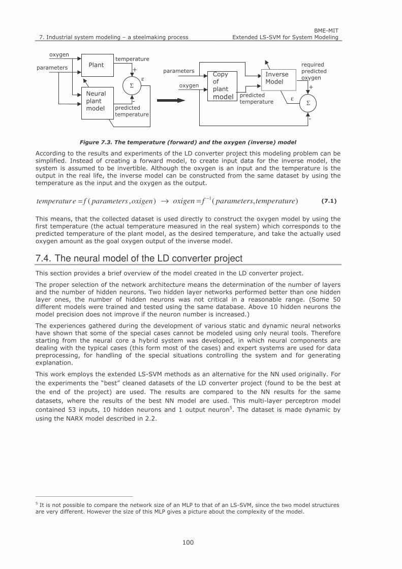
7. Industrial system modeling – a steelmaking process BME-MIT
Extended LS-SVM for System Modeling
100
Figure 7.3. The temperature (forward) and the oxygen (inverse) model
According to the results and experiments of the LD converter project this modeling problem can be simplified. Instead of creating a forward model, to create input data for the inverse model, the system is assumed to be invertible. Although the oxygen is an input and the temperature is the output in the real life, the inverse model can be constructed from the same dataset by using the temperature as the input and the oxygen as the output.
),( oxigenparametersfetemperatur = → ),(1etemperaturparametersfoxigen
−= (7.1)
This means, that the collected dataset is used directly to construct the oxygen model by using the first temperature (the actual temperature measured in the real system) which corresponds to the predicted temperature of the plant model, as the desired temperature, and take the actually used oxygen amount as the goal oxygen output of the inverse model.
7.4. The neural model of the LD converter project
This section provides a brief overview of the model created in the LD converter project.
The proper selection of the network architecture means the determination of the number of layers and the number of hidden neurons. Two hidden layer networks performed better than one hidden layer ones, the number of hidden neurons was not critical in a reasonable range. (Some 50 different models were trained and tested using the same database. Above 10 hidden neurons the model precision does not improve if the neuron number is increased.)
The experiences gathered during the development of various static and dynamic neural networks have shown that some of the special cases cannot be modeled using only neural tools. Therefore starting from the neural core a hybrid system was developed, in which neural components are dealing with the typical cases (this form most of the cases) and expert systems are used for data preprocessing, for handling of the special situations controlling the system and for generating explanation.
This work employs the extended LS-SVM methods as an alternative for the NN used originally. For the experiments the “best” cleaned datasets of the LD converter project (found to be the best at the end of the project) are used. The results are compared to the NN results for the same datasets, where the results of the best NN model are used. This multi-layer perceptron model contained 53 inputs, 10 hidden neurons and 1 output neuron5. The dataset is made dynamic by using the NARX model described in 2.2.
5 It is not possible to compare the network size of an MLP to that of an LS-SVM, since the two model structures are very different. However the size of this MLP gives a picture about the complexity of the model.
Plant
Neural plant model
Σ ε
parameters
temperature
predicted temperature
+
-
oxygen
oxygen
parameters
Σ ε
-
+
Inverse Model
predicted temperature
Copy of plant model
required predicted oxygen

7. Industrial system modeling – a steelmaking process BME-MIT
Extended LS-SVM for System Modeling
101
7.5. Validation method
After building the model –according to 7.3- from the measured dataset, the results must be validated. There are several options to do it, but the most important aspect of constructing a validation scheme is to simulate the real system and the real problem as close as possible.
In the real life situation, when the model is used the parameters collected at the end of the process are unknown. Only their desired values describing the steel required are known. This is an important difference, since in the training phase, the actual parameter values could be used, while in the validation phase (testing) the desired values of the same parameters are to be used. In the current modeling task, this distinction only stands for the steel temperature measured at the end of the production. In the model construction, the actual measured output temperature is used (
etemperaturfirst _ ); while in the model validation the originally desired goal temperature is
used. Of course this two temperature value is unlikely to be the same, since the personnel could not determine the optimal value of oxygen when the training data were collected. As it will be shown, the “small” difference between these temperatures will be accounted for in a linear manner. This is done, because according to prior knowledge provided by the steel making experts, a locally linear approximation can be used at this working point stating that an added 400 m3 oxygen results in +30 Celsius in the first temperature.
The temperature error of the model can be calculated according as follows:
1. The model is validated on loads, where the goal temperature is used as the temperature input.
2. The model provides an advised oxygen amount advised
O2 .
3. This advised oxygen amount is compared to the oxygen originally used, and the difference is converted into temperature using the locally linear approximation.
4. The calculated temperature difference is then added to the actual output temperature (first temperature) of the load. This value is the estimated temperature.
5. The estimated temperature is then compared to the goal temperature, ant the error is calculated.
The estimated temperature is calculated as follows:
etemperaturfirstOO
etemperaturestimatedadvised
_30400
_ 22 +−
= . (7.2)
To calculate the temperature error ( e_errortemperaturestimated_ ) for the advised oxygen (advised
O2 ) the estimated temperature ( etemperaturestimated _ ) should be compared to the
desired temperature goal ( etemperaturgoal _ ).
etemperaturgoaletemperaturestimatederroretemperaturestimated ____ −= (7.3)
It must be noted that there is a much simpler way to calculate the error, but it differs more from the actual real life situation. In this case the model is validated with the same temperature, namely the actual temperature measured ( etemperaturfirst _ ). This means that the
temperature parameter is not changed between the training and the validation phase which means, that the resulting oxygen estimation should meet the oxygen value of the sample. The oxygen error can be converted to a temperature error according to the locally linear rule described earlier.
Again it must be emphasized that in real life, the model can only be provided with the etemperaturgoal _ as an input – since there is no previously known etemperaturfirst _ in the
real life –, therefore the real capabilities of the inverse model are determined more precisely if the testing is done according to the previously described scheme, involving the temperature change between training and testing.

7. Industrial system modeling – a steelmaking process BME-MIT
Extended LS-SVM for System Modeling
102
In the experiments both error measures are used and they called simply:
With change (change) – The first temperature is changed to the goal temperature (aimed originally) when the error is calculated.
Without change (no change) – The first temperature is not changed to the goal temperature when the model is validated. The oxygen error is converted into temperature error.
It is clear that the error will be larger in the first case due to the use of the goal temperature. The change creates a sample where –if the first temperature is not the same as the goal- the linear model must be used, since the oxygen value of this sample corresponds to the first temperature. In most of the experiments both error measures are presented, but in case the error is not detailed, the more lifelike error measure, the one with the change is used.
7.6. Experiments
In this section the previously introduced industrial problem is used for testing the properties of the extended LS-SVM. It will be shown that the LS-SVM can produce better results than the traditional neural network based solution. The propositions of this paper for achieving sparseness and robustness are also tested and the results are compared to traditional LS-SVM and the neural results.
For the experiments the largest, most representative dataset of the LD converter project is used. This datasets were found as the most representative during the neural modeling, since it includes a large number of samples (even after filtering out the wrong samples) and also the best neural models where achieved for this dataset.
The dataset was collected, created, filtered and scaled during the original project. The dataset contains the data of three campaigns of the same converter as shown in Table 7.1.
Table 7.1. The LD converter dataset contains the data of three campaigns.
CAMPAIGN NUMBER OF SAMPLES
1 973
2 1859
3 1767
ΣΣΣΣ 4599
From the data of this three campaigns, two datasets where formed. The full dataset contains all the data collected. There are two samples missing, which where obvious errors and where filtered before normalization. From this dataset a filtered dataset is crated, which is filtered based on a large number of complex knowledge concerning the steelmaking process. In this case special loads (e.g. loads made to create special kinds of steel), and many other samples found somehow suspicious where removed. The filtering process and thus the datasets are the results of the former project.
Table 7.2. The normalized LD converter datasets used in the experiments.
DATASET NUMBER OF SAMPLES
Full dataset (filtered during normalization) 4597
Filtered dataset (leaving the samples that seem to have “large
error” based on prior knowledge)
2821
Based on this two dataset, the three experiments defined in Table 7.3 are made (based on the experiments available for the neural model).

7. Industrial system modeling – a steelmaking process BME-MIT
Extended LS-SVM for System Modeling
103
Table 7.3. Experimental setups used in the LD steel making problem.
SCHEME # METHOD TRAIN TEST DESCRIPTION
#1 Train and test for the split
full dataset.
3000 1597 The dataset is split to a train and test set, containing
3000 and 1597 samples respectively. Before splitting,
the dataset it is permuted (mixed) to have a random
train and test selection; therefore –due to this different
the train and test sets- there may be slight differences
in different experiments even for the same settings.
#2 Train and test for the split
filtered dataset.
2102 719 The dataset is split to a train and test set, containing
2102 and 719 samples respectively. The dataset was
split during the original project, thus this experiment is
exactly the same as the one used for the NN.
The original project created a neural model and the achieved best results are available for these datasets. Other research from literature concerning LD steel converter is available, but the results are very hard to compare mainly due to the differences of the used technology, the datasets (e.g. measured and used inputs, measurement precision etc.) and experimental setups (e.g. interpretation of error etc.). In general it can be stated, that any result around a 60% hit ratio is considered to be very good!
Due to the large number of samples, the experiments of this section take a very long time. In fact this was the original reason for starting to search for possible reduction methods. Due to this large algorithmic complexity, standard SVM cannot be used directly only if an iterative QP solver –such as SMO (see section 3.1.6)– is used. The experiments presented do not include SVM solutions, since this Thesis concerns LS-SVM and its extensions. Although LS-SVM and its extensions are significantly faster, such large datasets still have large memory and time requirements. This must be considered in designing the experiments in the sequel.
Since the LD converter project is finished already, our goal is not to create one optimal model for the problem, but to demonstrate the use and the main properties of the introduced methods on this real-life industrial problem.
In the experiments, it is shown; that the LS-SVM solution can be just as good as the results obtained with neural networks and are better than the 60% hit ratio known from literature. It is also shown, that LS2-SVM can also provide good results but with a sparse model. We also demonstrate that the robust solution can further improve the results on a dataset containing outliers.
It must be emphasized, that performance is not the only important aspect in selecting a modeling tool. Many other circumstances must be considered, such as
training time,
the difficulties of model construction,
the resulting model complexity and structure,
implementation issues etc..
As described in this Thesis, kernel methods and support vector based solutions have many advantages concerning these issues, thus they provide an important alternative to solve such problems.
To illustrate the LS-SVM and especially the extended LS-SVM on the LD converter problem, the following experiments are done:
The “optimal” hyper parameters (C and σ ) are determined.
The LS-SVM and LS2-SVM solutions are presented.
The trade of between sparseness and performance is demonstrated, thus the effect of the ε ′ tolerance value of the selection method proposed in 4.5.1 is examined.
The use of robust estimation is investigated on the dataset.

7. Industrial system modeling – a steelmaking process BME-MIT
Extended LS-SVM for System Modeling
104
7.6.1. Hyperparameter selection
This Thesis does not intend to provide methods for hyper parameter selection, but in order to solve the problem some good settings must be found. This is done by using cross validation.
The optimal parameters might be different for datasets collected from different campaigns and especially for ones collected from different (or rebuilt) converters. Since future steel production must be optimized, the goal of the original project was to create one model for all data (a general model of the whole process) one hyper parameter setting must be used for all the datasets.
The dataset used comes from three different campaigns of the same converter, but the model must work for all converters and campaigns. The best approach would be to use as many known data as possible –the whole sample set, containing 4597 samples– to optimize the settings, but that would mean a huge dataset, thus a very lengthy calculation. As cross-validation requires a large number of trials, this cannot be done. On the other hand, for demonstration it is enough to determine a setting that is “good enough”; therefore only 1000 data –selected randomly from the whole dataset- is used (this corresponds to scheme #1 described in Table 7.3 with less training vectors).
The optimal hyper-parameters are not the same for the LS-SVM and the LS2-SVM, since the sparse model is based on less Gaussians, which usually presumes a larger sigma (so that the kernels overlap), and a larger C (to have better generalization ability). In case of LS2-SVM, the optimal hyper parameter setting also depends on the degree of sparseness, thus the number of support vectors used. If the RREF based selection method is applied, this means, that the hyper parameters also depend on the ε ′ tolerance value used. The hyper parameters of the LS2-SVM is determined with a tolerance value of 0.01, which means a significant reduction, with only a small growth in the error (the exact values are shown later in section 7.6.2).
The C and σ hyper parameters are determined through cross validation in several steps (searches):
1. First a larger range of the parameters are searched.
2. Than several finer searches are run iteratively in the region around the previous minima.
Figure 7.4 shows the misclassification error surfaces for both LS-SVM and LS2-SVM. It can be seen, that the region of interest is more detailed due to the second search.
a.) b.)
Figure 7.4. The misclassification error rate plotted for different combinations of C and σ . The best
settings are at the minimum of these surfaces. a.) LS-SVM , b.) LS2-SVM.
The minima of these surfaces provide the estimations for of the hyper parameters.
0
5000
10000 0
5
1040
50
60
sigmaC
0
5000
10000 0
5
1040
50
60
70
sigmaC
σ σ

7. Industrial system modeling – a steelmaking process BME-MIT
Extended LS-SVM for System Modeling
105
The checked values are:
000,10000]100,2000,5900,1000,1
,550,800,90,500,510,200,400,420,150,180,100,110,11,10,80,90[∈C (7.4)
and
10]5,6,7,8,9,5,4.6,4.7,4.3,4.4,4.6,3.7,4.0,3.4,3.5,3.1,2,3,3.3,[∈σ . (7.5)
Table 7.4. The estimates for σ and C based on 1000 training samples.
LS-SVM LS2-SVM
ε ′ - 0.01
C 100 500
σ 3 3.7
Support vector # 1000 73
Misclassification error rate 41.7 % 41.7 %
The following figures (Figure 7.5 and Figure 7.6) show the misclassification error rates as a function of each of the hyper parameters, while the other parameter is fixed. This shows how the error depends on changing either one of the hyper parameters.
a.) b.)
Figure 7.5. The misclassification error rate of the original not pruned LS-SVM plotted for different
values of C and σ . The other parameter is fixed at the optimum a.) 3 =σ , b.) 100 C =
0 2000 4000 6000 8000 1000040
42
44
46
48
50
C0 2 4 6 8 10
41.5
42
42.5
43
43.5
44
44.5
sigmaσ
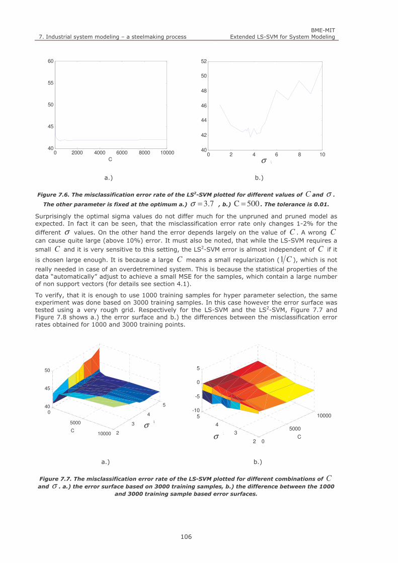
7. Industrial system modeling – a steelmaking process BME-MIT
Extended LS-SVM for System Modeling
106
a.) b.)
Figure 7.6. The misclassification error rate of the LS2-SVM plotted for different values of C and σ .
The other parameter is fixed at the optimum a.) 3.7 =σ , b.) 500 C = . The tolerance is 0.01.
Surprisingly the optimal sigma values do not differ much for the unpruned and pruned model as expected. In fact it can be seen, that the misclassification error rate only changes 1-2% for the different σ values. On the other hand the error depends largely on the value of C . A wrong C can cause quite large (above 10%) error. It must also be noted, that while the LS-SVM requires a small C and it is very sensitive to this setting, the LS2-SVM error is almost independent of C if it
is chosen large enough. It is because a large C means a small regularization ( C1 ), which is not
really needed in case of an overdetremined system. This is because the statistical properties of the data “automatically” adjust to achieve a small MSE for the samples, which contain a large number of non support vectors (for details see section 4.1).
To verify, that it is enough to use 1000 training samples for hyper parameter selection, the same experiment was done based on 3000 training samples. In this case however the error surface was tested using a very rough grid. Respectively for the LS-SVM and the LS2-SVM, Figure 7.7 and Figure 7.8 shows a.) the error surface and b.) the differences between the misclassification error rates obtained for 1000 and 3000 training points.
a.) b.)
Figure 7.7. The misclassification error rate of the LS-SVM plotted for different combinations of Cand σ . a.) the error surface based on 3000 training samples, b.) the difference between the 1000
and 3000 training sample based error surfaces.
0 2000 4000 6000 8000 1000040
45
50
55
60
C0 2 4 6 8 10
40
42
44
46
48
50
52
sigma
0
5000
10000 2
3
4
540
45
50
sigma
C
0
5000
10000
2
3
4
5-10
-5
0
5
Csigma
σ
σ
σ
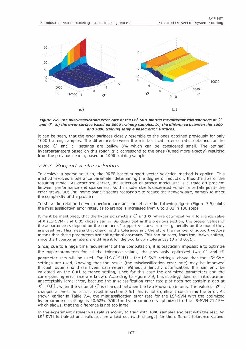
7. Industrial system modeling – a steelmaking process BME-MIT
Extended LS-SVM for System Modeling
107
a.) b.)
Figure 7.8. The misclassification error rate of the LS2-SVM plotted for different combinations of Cand σ . a.) the error surface based on 3000 training samples, b.) the difference between the 1000
and 3000 training sample based error surfaces.
It can be seen, that the error surfaces closely resemble to the ones obtained previously for only 1000 training samples. The difference between the misclassification error rates obtained for the tested C and σ settings are bellow 8% which can be considered small. The optimal hyperparameters based on this rough grid correspond to the ones (tuned more exactly) resulting from the previous search, based on 1000 training samples.
7.6.2. Support vector selection
To achieve a sparse solution, the RREF based support vector selection method is applied. This method involves a tolerance parameter determining the degree of reduction, thus the size of the resulting model. As described earlier, the selection of proper model size is a trade-off problem between performance and sparseness. As the model size is decreased –under a certain point- the error grows. But until some point it seems reasonable to reduce the network size, namely to meet the complexity of the problem.
To show the relation between performance and model size the following figure (Figure 7.9) plots the misclassification error rates, as tolerance is increased from 0 to 0.02 in 100 steps.
It must be mentioned, that the hyper parameters C and σ where optimized for a tolerance value of 0 (LS-SVM) and 0.01 chosen earlier. As described in the previous section, the proper values of these parameters depend on the number of support vectors, or more generally on the model they are used for. This means that changing the tolerance and therefore the number of support vectors means that these parameters are not optimal anymore. This can be seen, from the known optima, since the hyperparameters are different for the two known tolerances (0 and 0.01).
Since, due to a huge time requirement of the computation, it is practically impossible to optimize the hyperparameters for all the tolerance values, the previously optimized two C and σ
parameter sets will be used. For 01.00 ≤′≤ ε , the LS-SVM settings, above that the LS2-SVM settings are used, knowing that the result (the misclassification error rate) may be improved through optimizing these hyper parameters. Without a lengthy optimization, this can only be validated on the 0.01 tolerance setting, since for this case the optimized parameters and the corresponding error rate are known. According to Figure 7.9, this strategy does not introduce an unacceptably large error, because the misclassification error rate plot does not contain a gap at
01.0=′ε , when the value of C is changed between the two known optimums. The value of σ is changed as well, but as discussed in section 7.6.1 this is not significant concerning the error. As shown earlier in Table 7.4. the misclassification error rate for the LS2-SVM with the optimized hyperparameter settings is 20.62%. With the hyperparameters optimized for the LS-SVM 21.15% which shows, that the difference is not too large.
In the experiment dataset was split randomly to train with 1000 samples and test with the rest. An LS2-SVM is trained and validated on a test set (with change) for the different tolerance values.
0
5000
10000 23
45
40
45
50
55
60
sigmaC
0
5000
10000
2
3
4
5-10
-5
0
5
C
sigma
σ σ
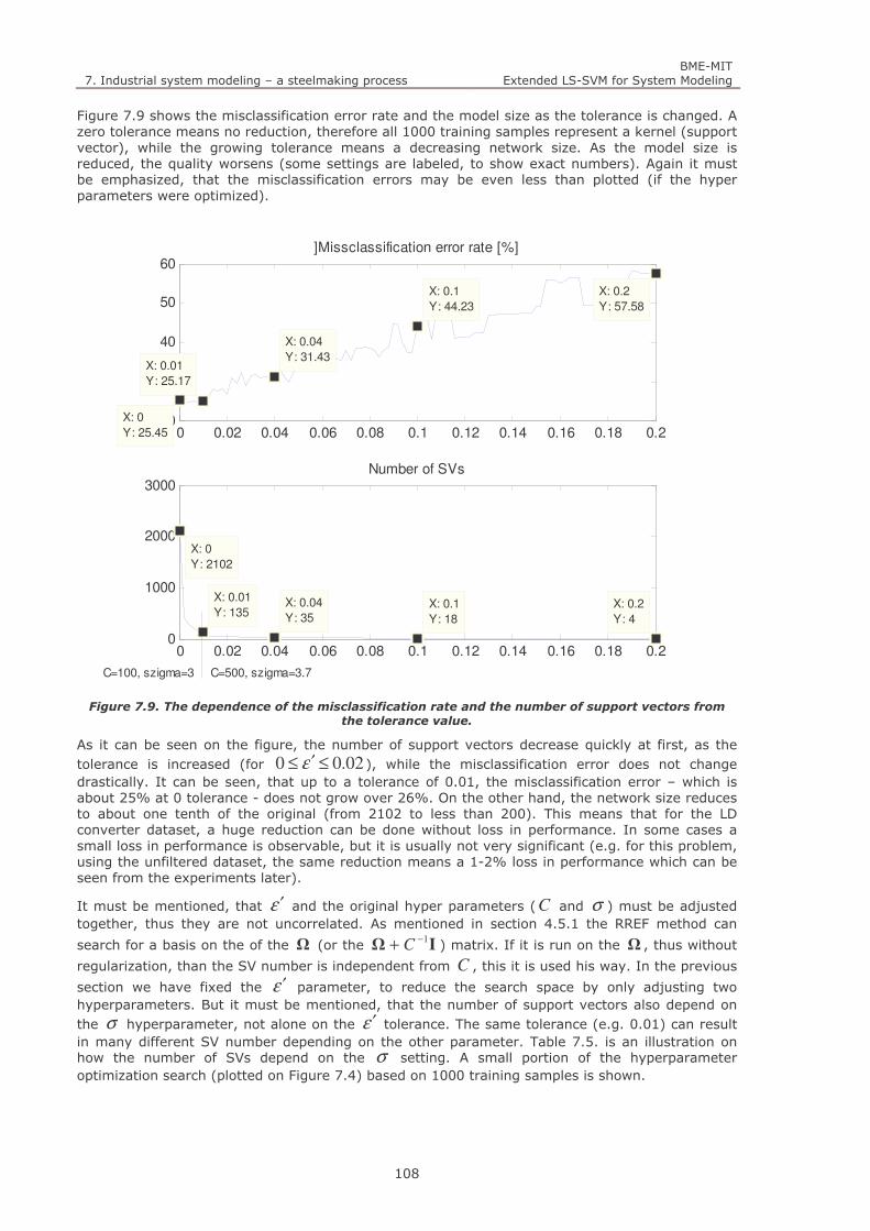
7. Industrial system modeling – a steelmaking process BME-MIT
Extended LS-SVM for System Modeling
108
Figure 7.9 shows the misclassification error rate and the model size as the tolerance is changed. A zero tolerance means no reduction, therefore all 1000 training samples represent a kernel (support vector), while the growing tolerance means a decreasing network size. As the model size is reduced, the quality worsens (some settings are labeled, to show exact numbers). Again it must be emphasized, that the misclassification errors may be even less than plotted (if the hyper parameters were optimized).
Figure 7.9. The dependence of the misclassification rate and the number of support vectors from
the tolerance value.
As it can be seen on the figure, the number of support vectors decrease quickly at first, as the tolerance is increased (for 02.00 ≤′≤ ε ), while the misclassification error does not change drastically. It can be seen, that up to a tolerance of 0.01, the misclassification error – which is about 25% at 0 tolerance - does not grow over 26%. On the other hand, the network size reduces to about one tenth of the original (from 2102 to less than 200). This means that for the LD converter dataset, a huge reduction can be done without loss in performance. In some cases a small loss in performance is observable, but it is usually not very significant (e.g. for this problem, using the unfiltered dataset, the same reduction means a 1-2% loss in performance which can be seen from the experiments later).
It must be mentioned, that ε ′ and the original hyper parameters (C and σ ) must be adjusted together, thus they are not uncorrelated. As mentioned in section 4.5.1 the RREF method can
search for a basis on the of the Ω (or the IΩ1−+ C ) matrix. If it is run on the Ω , thus without
regularization, than the SV number is independent from C , this it is used his way. In the previous
section we have fixed the ε ′ parameter, to reduce the search space by only adjusting two hyperparameters. But it must be mentioned, that the number of support vectors also depend on the σ hyperparameter, not alone on the ε ′ tolerance. The same tolerance (e.g. 0.01) can result in many different SV number depending on the other parameter. Table 7.5. is an illustration on how the number of SVs depend on the σ setting. A small portion of the hyperparameter optimization search (plotted on Figure 7.4) based on 1000 training samples is shown.
0 0.02 0.04 0.06 0.08 0.1 0.12 0.14 0.16 0.18 0.220
30
40
50
60
X: 0
Y: 25.45
X: 0.2
Y: 57.58
X: 0.1
Y: 44.23
X: 0.04
Y: 31.43X: 0.01
Y: 25.17
]Missclassification error rate [%]
0 0.02 0.04 0.06 0.08 0.1 0.12 0.14 0.16 0.18 0.20
1000
2000
3000
X: 0
Y: 2102
X: 0.01
Y: 135X: 0.04
Y: 35X: 0.1
Y: 18
X: 0.2
Y: 4
Number of SVs
C=100, szigma=3 C=500, szigma=3.7
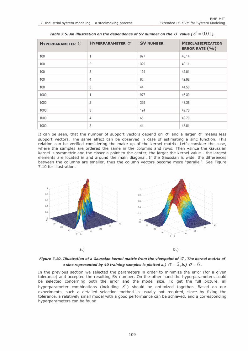
7. Industrial system modeling – a steelmaking process BME-MIT
Extended LS-SVM for System Modeling
109
Table 7.5. An illustration on the dependence of SV number on the σ value ( 01.0=′ε ).
HYPERPARAMETER C HYPERPARAMETER σ SV NUMBER MISCLASSIFICATION
ERROR RATE (%)
100 1 977 46.14
100 2 329 43.11
100 3 124 42.81
100 4 66 42.98
100 5 44 44.50
1000 1 977 46.39
1000 2 329 43.36
1000 3 124 42.73
1000 4 66 42.70
1000 5 44 43.81
It can be seen, that the number of support vectors depend on σ and a larger σ means less support vectors. The same effect can be observed in case of estimating a sinc function. This relation can be verified considering the make up of the kernel matrix. Let’s consider the case, where the samples are ordered the same in the columns and rows. Then –since the Gaussian kernel is symmetric and the closer a point to the center, the larger the kernel value - the largest elements are located in and around the main diagonal. If the Gaussian is wide, the differences between the columns are smaller, thus the column vectors become more “parallel”. See Figure 7.10 for illustration.
a.) b.)
Figure 7.10. Illustration of a Gaussian kernel matrix from the viewpoint of σ . The kernel matrix of
a sinc represented by 40 training samples is plotted a.) 2=σ ,b.) 6=σ .
In the previous section we selected the parameters in order to minimize the error (for a given tolerance) and accepted the resulting SV number. On the other hand the hyperparameters could be selected concerning both the error and the model size. To get the full picture, all hyperparameter combinations (including ε ′ ) should be optimized together. Based on our experiments, such a detailed selection method is usually not required, since by fixing the tolerance, a relatively small model with a good performance can be achieved, and a corresponding hyperparameters can be found.
0
10
20
30
40
0
10
20
30
400
0.2
0.4
0.6
0.8
1
0
10
20
30
40
0
10
20
30
400
0.2
0.4
0.6
0.8
1
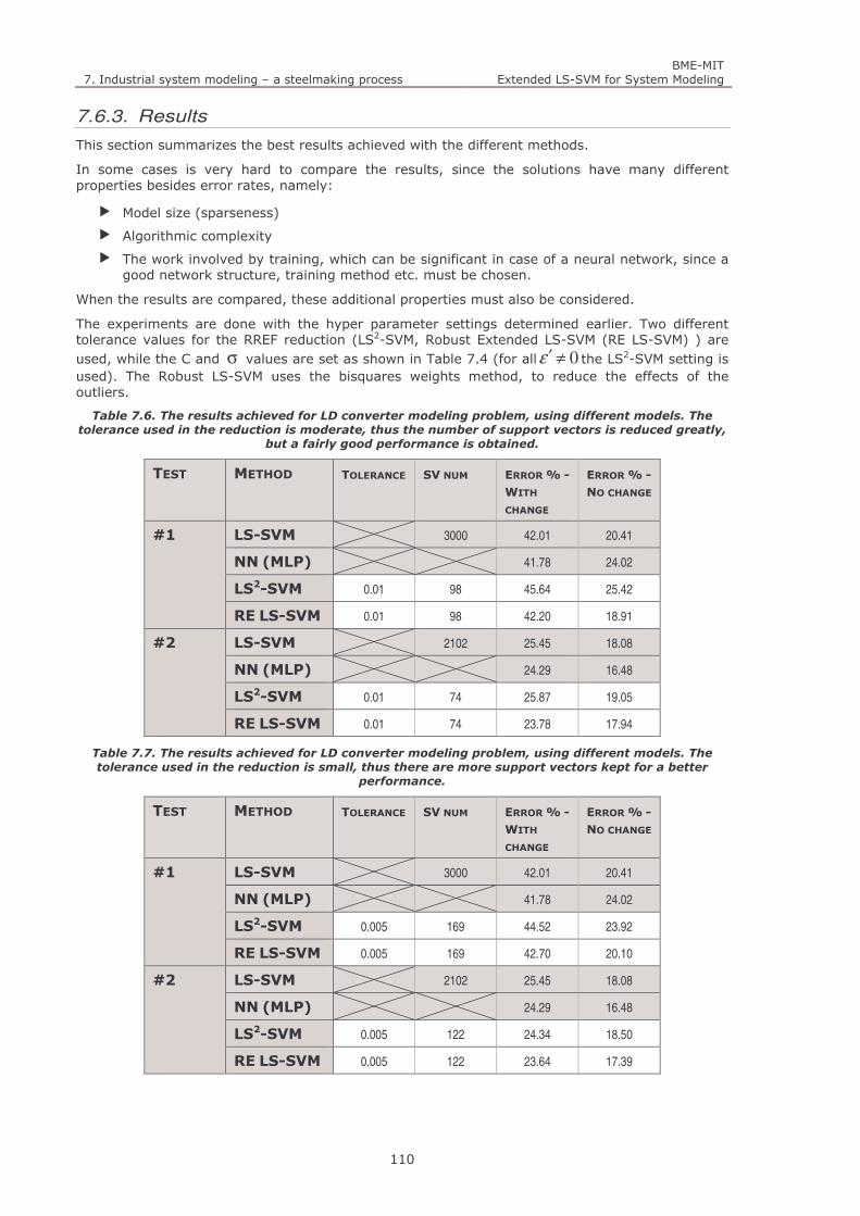
7. Industrial system modeling – a steelmaking process BME-MIT
Extended LS-SVM for System Modeling
110
7.6.3. Results
This section summarizes the best results achieved with the different methods.
In some cases is very hard to compare the results, since the solutions have many different properties besides error rates, namely:
Model size (sparseness)
Algorithmic complexity
The work involved by training, which can be significant in case of a neural network, since a good network structure, training method etc. must be chosen.
When the results are compared, these additional properties must also be considered.
The experiments are done with the hyper parameter settings determined earlier. Two different tolerance values for the RREF reduction (LS2-SVM, Robust Extended LS-SVM (RE LS-SVM) ) are used, while the C and σ values are set as shown in Table 7.4 (for all 0≠′ε the LS2-SVM setting is used). The Robust LS-SVM uses the bisquares weights method, to reduce the effects of the outliers.
Table 7.6. The results achieved for LD converter modeling problem, using different models. The
tolerance used in the reduction is moderate, thus the number of support vectors is reduced greatly,
but a fairly good performance is obtained.
TEST METHOD TOLERANCE SV NUM ERROR % -
WITH
CHANGE
ERROR % -
NO CHANGE
#1 LS-SVM 3000 42.01 20.41
NN (MLP) 41.78 24.02
LS2-SVM 0.01 98 45.64 25.42
RE LS-SVM 0.01 98 42.20 18.91
#2 LS-SVM 2102 25.45 18.08
NN (MLP) 24.29 16.48
LS2-SVM 0.01 74 25.87 19.05
RE LS-SVM 0.01 74 23.78 17.94
Table 7.7. The results achieved for LD converter modeling problem, using different models. The
tolerance used in the reduction is small, thus there are more support vectors kept for a better
performance.
TEST METHOD TOLERANCE SV NUM ERROR % -
WITH
CHANGE
ERROR % -
NO CHANGE
#1 LS-SVM 3000 42.01 20.41
NN (MLP) 41.78 24.02
LS2-SVM 0.005 169 44.52 23.92
RE LS-SVM 0.005 169 42.70 20.10
#2 LS-SVM 2102 25.45 18.08
NN (MLP) 24.29 16.48
LS2-SVM 0.005 122 24.34 18.50
RE LS-SVM 0.005 122 23.64 17.39

7. Industrial system modeling – a steelmaking process BME-MIT
Extended LS-SVM for System Modeling
111
Table 7.8. The results achieved for LD converter modeling problem, using different models. In this
case the tolerance is too large, resulting in a very few SVs and consequently unacceptable large
errors.
TEST METHOD TOLERANCE SV NUM ERROR % -
WITH
CHANGE
ERROR % -
NO CHANGE
#1 LS-SVM 3000 42.01 20.41
NN (MLP) 41.78 24.02
LS2-SVM 0.1 23 53.48 39.39
RE LS-SVM 0.1 23 51.9 35.13
#2 LS-SVM 2102 25.45 18.08
NN (MLP) 24.29 16.48
LS2-SVM 0.1 18 44.23 40.47
RE LS-SVM 0.1 18 40.61 35.46
It can be seen, that the LS2-SVM can produce good results with significantly smaller models. The robust versions bring a slight improvement in the result. To have a robust solution it is necessary to reduce complexity, therefore this result should be primarily compared to the LS2-SVM. On the other hand, if outliers are present in the dataset, that affects the LS-SVM result as well, therefore even this result may be improved by using a robust method. This is even more conspicuous if the “no change” error measure is considered, since in this case, the error of the dataset –the difference between goal first and the achieved first temperature- does not alter the results.
Since there is limited information about the dataset concerning the amount of noise, in order to demonstrate the robust method, some outliers are inserted into the dataset. Table 7.9 shows the result obtained for this modified a dataset, where 10 training samples are corrupted. The tables do not contain NN results, since the goal of these experiments is to show, how the outliers corrupt the results if there is no robustness incorporated in the solution, but with robust methods, the effects of these corrupted samples are suppressed. Again the LS-SVM results do not change for the different tolerance settings, but the results are repeated in each table for convenient comparison. The experiments follow the ones above, but the too large tolerance setting is not included, since due to the extensive reduction, the results are too bad in the first place.
Table 7.9. The results achieved for a corrupted LD converter modeling dataset, using different
models. The tolerance used for reduction is moderate: 01.0=′ε .
TEST METHOD TOLERANCE SV NUM ERROR % -
WITH
CHANGE
ERROR % -
NO CHANGE
#1 LS-SVM 3000 43.14 21.91
LS2-SVM 0.01 98 46.71 26.29
RE LS-SVM 0.01 98 42.20 18.85
#2 LS-SVM 2102 28.37 21.14
LS2-SVM 0.01 74 29.21 20.44
RE LS-SVM 0.01 74 23.5 17.80
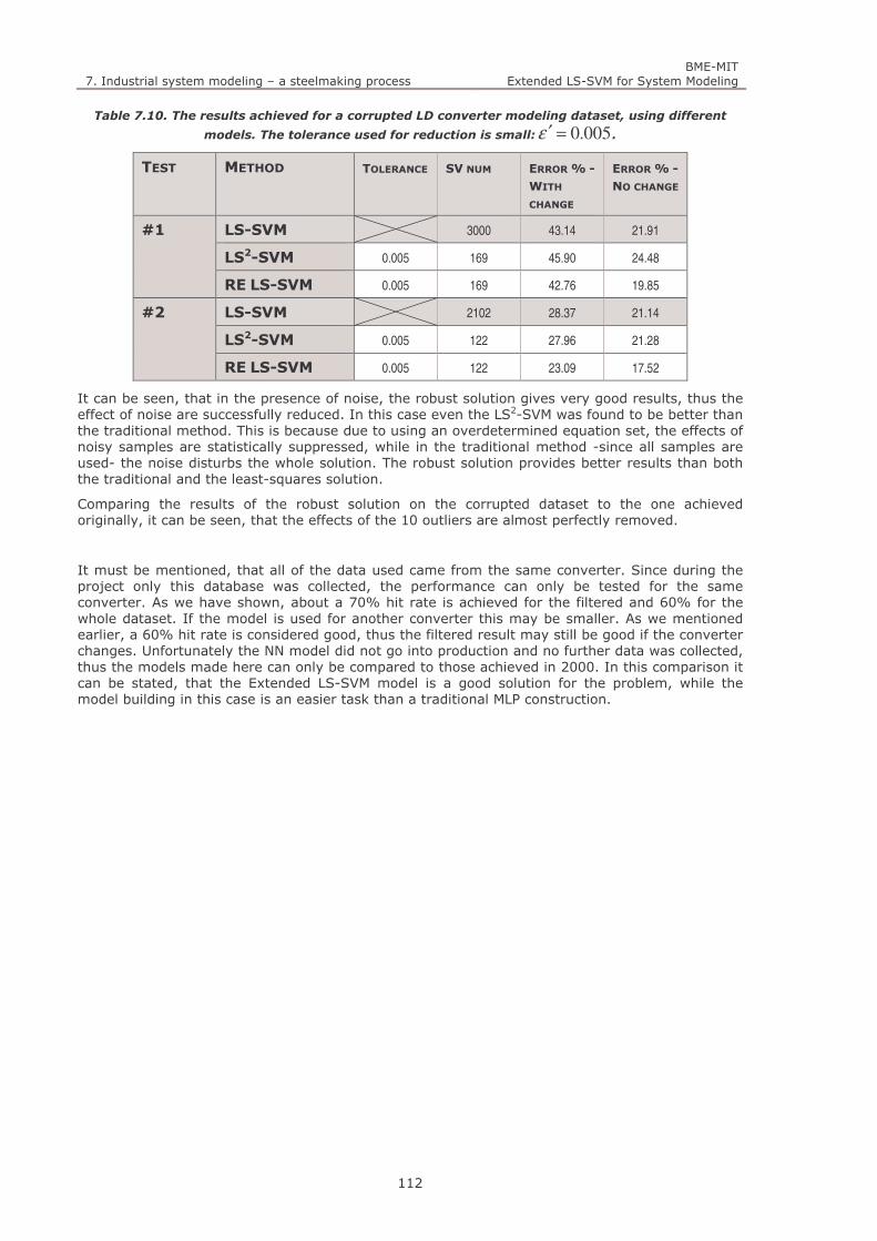
7. Industrial system modeling – a steelmaking process BME-MIT
Extended LS-SVM for System Modeling
112
Table 7.10. The results achieved for a corrupted LD converter modeling dataset, using different
models. The tolerance used for reduction is small: 005.0=′ε .
TEST METHOD TOLERANCE SV NUM ERROR % -
WITH
CHANGE
ERROR % -
NO CHANGE
#1 LS-SVM 3000 43.14 21.91
LS2-SVM 0.005 169 45.90 24.48
RE LS-SVM 0.005 169 42.76 19.85
#2 LS-SVM 2102 28.37 21.14
LS2-SVM 0.005 122 27.96 21.28
RE LS-SVM 0.005 122 23.09 17.52
It can be seen, that in the presence of noise, the robust solution gives very good results, thus the effect of noise are successfully reduced. In this case even the LS2-SVM was found to be better than the traditional method. This is because due to using an overdetermined equation set, the effects of noisy samples are statistically suppressed, while in the traditional method -since all samples are used- the noise disturbs the whole solution. The robust solution provides better results than both the traditional and the least-squares solution.
Comparing the results of the robust solution on the corrupted dataset to the one achieved originally, it can be seen, that the effects of the 10 outliers are almost perfectly removed.
It must be mentioned, that all of the data used came from the same converter. Since during the project only this database was collected, the performance can only be tested for the same converter. As we have shown, about a 70% hit rate is achieved for the filtered and 60% for the whole dataset. If the model is used for another converter this may be smaller. As we mentioned earlier, a 60% hit rate is considered good, thus the filtered result may still be good if the converter changes. Unfortunately the NN model did not go into production and no further data was collected, thus the models made here can only be compared to those achieved in 2000. In this comparison it can be stated, that the Extended LS-SVM model is a good solution for the problem, while the model building in this case is an easier task than a traditional MLP construction.

8. Summary of new scientific results BME-MIT
Extended LS-SVM for System Modeling
113
8. SUMMARY OF NEW SCIENTIFIC RESULTS
The first Thesis proposes a special “partial reduction” technique, where the LS-SVM training equation set is reformulated to describe a sparse, but precise model and algorithmically more effective problem. In Thesis 2 some methods are proposed to support the reduction, thus to select the support vectors. It is also shown, that traditional methods can also be used in conjunction with the partial reduction method. The reduced equation set can be solved using different techniques to achieve more general, e.g. robust estimates. These possible solution methods are summarized by Thesis 3.
1. Thesis: I have developed a new partially reduced LS-SVM formulation, which provides a sparse solution (reduced model complexity), but still uses all training
samples to construct the model; therefore the reduction infers minimal performance degradation, compared to the unreduced (full sized) LS-SVM.
1.1. I have shown that partial reduction leads to a sparse LS-SVM model, but at the same time preserves all known information (constraints), provided by the training dataset, to construct the solution.
1.2. I have shown that the sparse solution constructed by partial reduction –since all samples are considered- can perform better, than the model constructed by traditional pruning, which entirely omits some samples. On the other hand, the same performance can be achieved by a smaller model.
1.3. Simulations show that in case of partial reduction the effect of regularization is changed, because it is not the only term responsible for avoiding overfitting (thus to achieve good generalization).
1.4. I have shown that the partially reduced LS-SVM, which is derived from the original LS-SVM formulation, corresponds to a model that applies the regularization in the kernel space (instead of the feature space).
2. Thesis: I have proposed new methods that can be used to select the support vectors of the partially reduced model and I have shown that other known methods can also
be utilized –with only slight changes– for this task.
2.1. I have proposed a new effective support vector selection method. Similarly to the traditional SVM, this algorithm incorporates a tolerance parameter which controls the trade off between the model size (sparseness) and performance. The proposed method is algorithmically effective compared to the known –mostly iterative– methods. Using simulations, I have shown that this method leads to good results concerning model performance.
2.2. I have shown that previously published selection methods (such as FVS, traditional LS-SVM pruning etc.) can be applied to select the support vectors with only a slight change.
2.3. I have shown that in correspondence with the traditional Fixed Size LS-SVM, partial reduction can also be utilized to create a fixed size LS-SVM model, whilst the good properties of this method are preserved.
2.4. I have shown that a new inverse pruning method can be achieved by using the opposite of the selection criteria used by the traditional pruning method. Using simulations, I have shown that in case of certain hyper parameter settings this method leads to better results than the traditional pruning method.
3. Thesis: I have shown that since the partially reduced LS-SVM leads to an
overdetermined system –in the kernel space- the problem can be further analyzed,

8. Summary of new scientific results BME-MIT
Extended LS-SVM for System Modeling
114
and optimized solutions (especially ones that reduce the effects of noise) can be found.
3.1. I have shown that, if the noise corrupting each training sample is known, than a weighted least-squares solution can provide the optimal solution.
3.2. I have shown that traditional pruning and weighting – although their goals do not rule out each other – cannot be used at the same time, because they work in opposition. The extended LS-SVM is capable of achieving both goals (thus a sparse and robust solution) simultaneously.
3.3. I have shown that applying linear regression methods of robust statistics in the kernel space can reduce, or remove the effects of noise, especially the effects of outliers.
3.4. I have shown that the approximation problem in the kernel space can be further generalized, by allowing locally linear or even nonlinear solutions. The locally linear models permit incremental learning, while the nonlinear solution, in the case when an LS-SVM or SVM is used for the kernel space regression, can lead to a multi layer LS-SVM.
9. Conclusions, Future Research BME-MIT
Extended LS-SVM for System Modeling
115
9. CONCLUSIONS, FUTURE RESEARCH
This Thesis extended the formulation of LS-SVMs in order to make them more applicable for large and erroneous datasets, thus real-life industrial problems. It also provides some viewpoints, and new approaches that can help to enlighten the similarities, special features and common grounds behind kernel based approaches like Ridge Regression, Kernel Ridge Regression, LS-SVM and SVMs. The modifications proposed are based on simple mathematical backgrounds and relate many existing and new ideas to create extended LS-SVM formulations to exploit the potentials of this field.
At the end of this Thesis, this chapter gives a brief overview of open questions and some new ideas that remained unexplored and can be addressed in future works.
The most important and interesting research areas considered currently:
The selection of hyper parameters, including the ε ′ tolerance introduced by the proposed SV selection method.
Custom weighted approaches for robust solutions of the overdetermined system, that guarantee good results, for different problem scenarios.
Bounds for the generalization error of LS-SVM and LS2-SVM solutions.
The relation between sparseness and expected error.
The properties of inverse pruning.
Support vector selection methods, focusing on a method that also considers the desired output when selecting SVs.
The possibilities of using a nonlinear approximation in the kernel space.

10. Appendix BME-MIT
Extended LS-SVM for System Modeling
116
10. APPENDIX
10.1. Properties of datasets
As described in the introduction the data set, describing the problem, may pose several problems to the user [28]:
noisy data – which means that the samples are unreliable and may be misleading.
non-uniformly distributed samples – resulting in under and overrepresented regions in the problem domain.
missing data – the data vectors may contain missing elements or whole samples may be missing.
too small or too large datasets – causing training difficulties.
etc..
As the dataset should describe the whole process thoroughly and precisely, almost all real-life problems contain these difficulties.
These problems are usually dealt with using preprocessing methods (filtering, data cleaning etc.), but in most cases the applied modeling method must also be able to handle such problems. This Thesis aim at reducing or eliminating the effects of noise.
When a black-box modeling method is described, it is very important to characterize our data concerning its quality. In most cases – e.g. in industrial modeling – the data are usually measured, therefore corrupted by noise. In order to minimize the undesirable effects of the noise one must consider it when building the model. Sometimes there is some prior information about the noise, but there are cases, when assumptions must be made.
Besides having noisy measurements, the training dataset may include some “totally” wrong samples, called outliers. In statistics, an outlier is a single observation “far away” from the rest of the data.
The methods discussed in this Thesis aim at reducing the effects of noise, in the following situations:
There is no knowledge about the noise. In this case the noise is usually assumed to be of a zero mean normal distribution (see later in 10.1.1).
There is some prior information available about the noise. This knowledge can be used in model construction.
There are some outliers in the training samples. As it will be shown, the most interesting problem is to detect outliers among the desired outputs (see 10.1.2).
For successful system modeling both the effects of noise (from a certain distribution) and the effects of outliers must be reduced!
10.1.1. Noisy data
When the properties of noise corrupting the training data are unknown, one can assume that there is not a unique significant source or cause of it. This means that the noise is originating in many different sources and the resulting noise is the sum of these. In system modeling problems, the noise is mostly considered to be of Gaussian, because -according to the central limit theorem- under certain conditions, the distribution of a sum of a large number of independent variables is approximately normal.
10. Appendix BME-MIT
Extended LS-SVM for System Modeling
117
In some cases however there are some prior information available regarding the noise. When the training data are collected, many different input and output values are measured, collected, by various methods. The amount of noise, corrupting a certain input or output, is often known or can be estimated from the physical properties of the used method. In these cases this additional information should be used in the model construction. This additional information is usually embodied in a weighted dataset, where the weighting factor iw reflects the quality (and thus the importance) of each sample. The more precise (less noisy) samples should have large weights, as being important. On the contrary, samples with large errors should have small weights, as they are more misleading and therefore should be considered as being less important.
N
iiii
traindw
1,,
==Ζ x . (10.1)
In some cases the standard deviation of the noise corrupting the input iσ is available (which is
motivated by similar reasons described above)
N
iiiitrain d 1,, ==Ζ σx . (10.2)
10.1.2. Outliers
In most datasets, some data points will be further away from their expected values than what seems reasonable.
An observation (or measurement) that is unusually large or small relative to the other
values in a data set is called an outlier.
Outliers can be detected on the uncorrelated, independent input components, since mostly there is some domain knowledge available about the specific measurement (e.g. valid values, range, measurement errors etc.). On the other hand, the output of the system cannot be handled similarly, since it is correlated to the inputs by definition. As long as the input-output relationship is unknown, it is very hard to determine which samples are outliers on the output, since it can only be interpreted in the context of the result (estimated model).
Outliers defined
In statistics, the precise definition of an outlier is based on the term inter quartile range, which is defined as follows.
In descriptive statistics the data set is sorted, and then split to four equal parts, so that each part represents one fourth of the samples. A quartile is any of the three values which divide the data set into four equal parts.
Thus:
first quartile ( 1Q )= lower quartile = cuts off lowest 25% of the data
second quartile ( 2Q )= median = cuts data set in half
third quartile ( 3Q )= upper quartile = cuts off highest 25% of the data, or the lowest
75%
The difference between the upper and lower quartiles is called the inter quartile range (IQR).
Mild Outliers
Using the definitions above, 1L and 1U define the so-called inner fences:
IQRQL ×−= 5.111 and IQRQU ×+= 5.131 , (10.3)
beyond which ( 1L< or 1U> ) an observation would be labeled as a mild outlier.
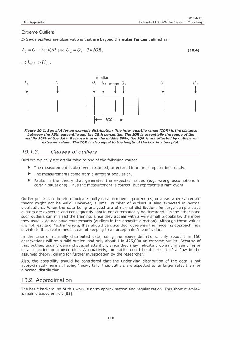
10. Appendix BME-MIT
Extended LS-SVM for System Modeling
118
Extreme Outliers
Extreme outliers are observations that are beyond the outer fences defined as:
IQRQL ×−= 312 and IQRQU ×+= 332 , (10.4)
( 2L< or 2U> ).
Figure 10.1. Box plot for an example distribution. The inter quartile range (IQR) is the distance
between the 75th percentile and the 25th percentile. The IQR is essentially the range of the
middle 50% of the data. Because it uses the middle 50%, the IQR is not affected by outliers or
extreme values. The IQR is also equal to the length of the box in a box plot.
10.1.3. Causes of outliers
Outliers typically are attributable to one of the following causes:
The measurement is observed, recorded, or entered into the computer incorrectly.
The measurements come from a different population.
Faults in the theory that generated the expected values (e.g. wrong assumptions in certain situations). Thus the measurement is correct, but represents a rare event.
Outlier points can therefore indicate faulty data, erroneous procedures, or areas where a certain theory might not be valid. However, a small number of outliers is also expected in normal distributions. When the data being analyzed are of normal distribution, for large sample sizes outliers are expected and consequently should not automatically be discarded. On the other hand such outliers can mislead the training, since they appear with a very small probability, therefore they usually do not have counterparts (outliers in the opposite direction). Although these values are not results of “extra” errors, they should be discarded, otherwise the modeling approach may deviate to these extremes instead of keeping to an acceptable “mean” value.
In the case of normally distributed data, using the above definitions, only about 1 in 150 observations will be a mild outlier, and only about 1 in 425,000 an extreme outlier. Because of this, outliers usually demand special attention, since they may indicate problems in sampling or data collection or transcription. Alternatively, an outlier could be the result of a flaw in the assumed theory, calling for further investigation by the researcher.
Also, the possibility should be considered that the underlying distribution of the data is not approximately normal, having "heavy tails, thus outliers are expected at far larger rates than for a normal distribution.
10.2. Approximation
The basic background of this work is norm approximation and regularization. This short overview is mainly based on ref. [83].
median
2Q 2U2L 1L
IQR
mean 3Q 1U1Q
10. Appendix BME-MIT
Extended LS-SVM for System Modeling
119
The simplest norm approximation problem is an unconstrained problem of the form
bAx −min (10.5)
where MN×ℜ∈A and Nℜ∈b are the data describing the problem (in our scenario they are the
N training inputs and the corresponding desired outputs respectively), Mℜ∈x is the variable
(in our case it is usually the weight vector) and . is a norm on Mℜ .
The vector
bAx −=r (10.6)
is the residual for the problem. The components of this vector are the residuals for x .
The norm approximation problem is a solvable convex optimization problem, with at least one optimal solution. The residual of the optimal solution is zero if and only if b can be produced as the linear combination of the columns of A , otherwise the error –the residuals- must really be minimized.
If NM = the optimal solution is bAx 1−= . If MN > we will assume that the columns of A are independent, without loss of generality.
The problem can be expressed as follows:
MMxx aaAx ++= L11 (10.7)
where M
n R∈aa ,...,1 are the columns of A ant the ix -s are the components of x . It can be
seen, that the norm approximation problem is can be interpreted as expressing the vector b as the linear combination of the column vectors of A . In this case, the columns of A are the repressors, and the result of (10.6) is the regression of b .
This regression problem interpretation will be used throughout this Thesis since this fits the best to the contents.
10.2.1. Least-squares approximation (linear regression)
The most common norm used by approximation problems is the 2l -norm. This norm squares our
objective and leads to a least-squares approximation problem.
∑=
==−N
i
irr1
22
2
2
2min bAx (10.8)
The optimal x solution of this problem must satisfy the normal equations
bAAxATT = . (10.9)
Since we assume, that the columns of A are independent, there is one unique solution:
bAAAx TT 1)( −= . (10.10)
The dimensionality of A is MN × , but AAT is MM × , and bAT is 1×M .
10. Appendix BME-MIT
Extended LS-SVM for System Modeling
120
10.2.2. Weighted approximation
The weighted norm approximation problem involves a weighting matrix, which modifies the optimization problem:
)(min bAxW − (10.11)
where the NN×ℜ∈W is often diagonal and in this case expresses the relative importance of the different components of the residual vector. This can be interpreted as a norm approximation
problem, with norm . , and data WAA =′ and Wbb =′ .
10.2.3. Regularization
Regularization is a very common method, to handle problems, where an added optimization criteria should also be considered. To scalarize the problem often the weighted sum of the objectives is minimized:
bAxx -C+ minimize , (10.12)
where 0>C is a trade of parameter between the goals. Another common method (especially when Euclidean norm is used) is to use squared norms in the weighted sum:
22 minimize bAxx -C+ , (10.13)
These regularization methods allow us to find a solution where the approximation error bAx-
and 2
x are optimized simultaneously.
10.2.4. Tikhonov regularization
Tikhonov regularization [61],[62] is the most commonly used method of regularization of ill-posed problems. It is based on (10.13), with Euclidean norms:
bbAxbxIAAxbAxx TTTT
C-C +−+=+ 2)
1(
2
1 minimize
22, (10.14)
where I is the NN × identity matrix. This problem has the following analytical solution:
In case A is quadratic this can be reduced to a simpler form:
Thanks to the 0>C regularization parameter, this least-squares solution always exists without any assumptions on the rank of A (like being nonsingular).
For 0=C this problem reduces to the least-squares approximation (shown in section 10.2.1) if
MN > .
bAIAAx TT
C
1)1
( −+= . (10.15)
bIAx 1)1
( −+=C
. (10.16)
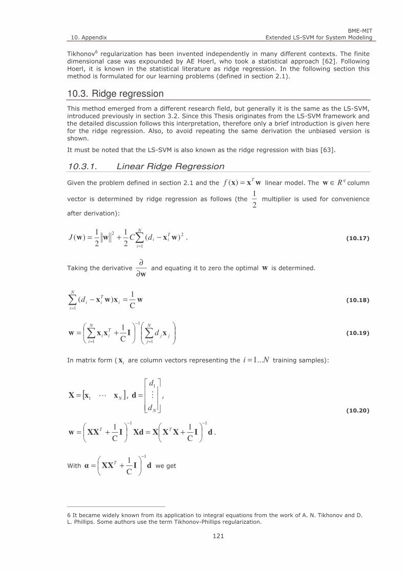
10. Appendix BME-MIT
Extended LS-SVM for System Modeling
121
Tikhonov6 regularization has been invented independently in many different contexts. The finite dimensional case was expounded by AE Hoerl, who took a statistical approach [62]. Following Hoerl, it is known in the statistical literature as ridge regression. In the following section this method is formulated for our learning problems (defined in section 2.1).
10.3. Ridge regression
This method emerged from a different research field, but generally it is the same as the LS-SVM, introduced previously in section 3.2. Since this Thesis originates from the LS-SVM framework and the detailed discussion follows this interpretation, therefore only a brief introduction is given here for the ridge regression. Also, to avoid repeating the same derivation the unbiased version is shown.
It must be noted that the LS-SVM is also known as the ridge regression with bias [63].
10.3.1. Linear Ridge Regression
Given the problem defined in section 2.1 and the wxx Tf =)( linear model. The q
R∈w column
vector is determined by ridge regression as follows (the 2
1 multiplier is used for convenience
after derivation):
Taking the derivative w∂
∂ and equating it to zero the optimal w is determined.
In matrix form ( ix are column vectors representing the Ni ...1= training samples):
With dIXXα
1
C
1−
+= T we get
6 It became widely known from its application to integral equations from the work of A. N. Tikhonov and D. L. Phillips. Some authors use the term Tikhonov-Phillips regularization.
∑=
−+=N
i
TiidCJ
1
22)(
2
1
2
1)( wxww . (10.17)
wxwxC
1 )(
1
=−∑=
N
i
i
T
iid (10.18)
+= ∑∑
=
−
=
N
j
jj
N
i
T
ii d1
1
1 C
1xIxxw (10.19)
[ ]NxxX L1= ,
=
Nd
d
M
1
d ,
dIXXXXdIXXw
11
C
1
C
1−−
+=
+= TT .
(10.20)
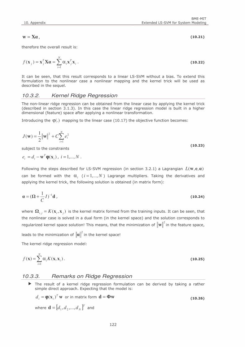
10. Appendix BME-MIT
Extended LS-SVM for System Modeling
122
therefore the overall result is:
It can be seen, that this result corresponds to a linear LS-SVM without a bias. To extend this formulation to the nonlinear case a nonlinear mapping and the kernel trick will be used as described in the sequel.
10.3.2. Kernel Ridge Regression
The non-linear ridge regression can be obtained from the linear case by applying the kernel trick (described in section 3.1.3). In this case the linear ridge regression model is built in a higher dimensional (feature) space after applying a nonlinear transformation.
Introducing the (.)ϕ mapping to the linear case (10.17) the objective function becomes:
Following the steps described for LS-SVM regression (in section 3.2.1) a Lagrangian ),,( αewL
can be formed with the iα ( Ni ,...,1= ) Lagrange multipliers. Taking the derivatives and
applying the kernel trick, the following solution is obtained (in matrix form):
where ),(, jiji K xxΩ = is the kernel matrix formed from the training inputs. It can be seen, that
the nonlinear case is solved in a dual form (in the kernel space) and the solution corresponds to
regularized kernel space solution! This means, that the minimization of 2
w in the feature space,
leads to the minimization of 2
α in the kernel space!
The kernel ridge regression model:
10.3.3. Remarks on Ridge Regression
The result of a kernel ridge regression formulation can be derived by taking a rather simple direct approach. Expecting that the model is:
where [ ]T
Nddd ,...,, 21=d and
Xαw = , (10.21)
∑=
α==N
i
i
T
ji
T
jjf1
)( xxXαxx . (10.22)
∑=
+=N
i
ieCJ1
22
2
1)( ww
subject to the constraints
)( i
T
ii de xw ϕϕϕϕ−= , Ni ,...,1= .
(10.23)
dΩα1)
1( −+= I
C, (10.24)
∑=
α=N
i
ii Kf1
),()( xxx . (10.25)
wxT
iid )(ϕϕϕϕ= or in matrix form Φwd = (10.26)
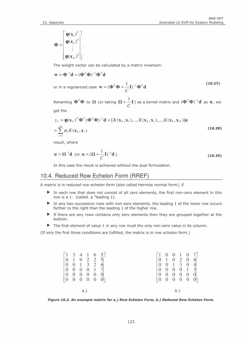
10. Appendix BME-MIT
Extended LS-SVM for System Modeling
123
=
T
N
T
T
)(
)(
)(
2
1
x
x
x
Φ
ϕϕϕϕ
ϕϕϕϕ
ϕϕϕϕ
M.
The weight vector can be calculated by a matrix inversion:
Renaming ΦΦT to Ω (or taking IΩ
C
1+ ) as a kernel matrix and dΦΦ
1)( −T as α , we
get the
result, where
In this case the result is achieved without the dual formulation.
10.4. Reduced Row Echelon Form (RREF)
A matrix is in reduced row echelon form (also called Hermite normal form), if
In each row that does not consist of all zero elements, the first non-zero element in this row is a 1. (called. a "leading 1).
In any two successive rows with non-zero elements, the leading 1 of the lower row occurs farther to the right than the leading 1 of the higher row.
If there are any rows contains only zero elements then they are grouped together at the bottom.
The first element of value 1 in any row must the only non-zero value in its column.
(If only the first three conditions are fulfilled, the matrix is in row echelon form.)
000000000000710000623100522910561431
000000000000310000403100602010701001
a.) b.)
Figure 10.2. An example matrix for a.) Row Echelon Form, b.) Reduced Row Echelon Form.
dΦΦΦdΦw TT 11 )( −− ==
or in a regularized case dΦIΦΦw TT
C
1)1
( −+= (10.27)
∑=
−
=
==N
i
iki
NkikkTTT
kk
K
KKKy
1
11
),(
)],(),...,,(),...,,([)()(
xx
αxxxxxxdΦΦΦx
α
ϕϕϕϕ
(10.28)
dΩα1−= (or dIΩα
1)1
( −+=C
). (10.29)

10. Appendix BME-MIT
Extended LS-SVM for System Modeling
124
10.5. Iterative solution to LS-SVM
In case of large datasets, iterative solutions, such as the conjugate gradient algorithm may be used to construct the LS-SVM model as described in section 3.2.4.
The conjugate gradient method requires the matrix to be positive definite. To iteratively solve an bAx = linear system, with a positive definite A the
bxAxxx TTJ −=
2
1)( (10.30)
cost function is used, where the solution of the corresponding equation set can be found by
)(minarg xx
J . (10.31)
In the Heistens-Stiefel conjugate gradient algorithm (its use is proposed by Suykens [13]), one
starts from an initial 0x and then )( iJ x is decreased iteratively. The details of this algorithm
can be found in ref. [13].
The use of iterative algorithms to solve large scale linear systems is preferred over the use of
direct methods, since they would involve a computational complexity of )( 3NO and memory
requirements of )( 2NO . The computational complexity of the CG algorithm is at most )( 2NrO c
when A is stored, where cr is the rank of C from CIA += . The number of required
iterations is typically smaller than cr , an additional reduction in the computational requirements
is obtained. When the matrix A is too large to be stored in memory, it can be recomputed in
each iteration, which costs an additional )( 2NO operations per step, but on the other hand
reduces the memory requirements to )(NO [14].
To apply the CG methods the equation set must first be modified, to reach a linear system with a positive definite matrix.
The LS-SVM system –in case of classification– is:
=
+ − 1αIΩdd r00
1b
C
T
, T
Nddd ],...,,[ 21=d , T
N ],..,,[ 21 ααα=α , T]1,...,1[=1r
,
),(, jijiji Kdd xx=Ω .
(10.32)
This can be transformed into:
=
+
−
−1
1HddHαH0
0 r
r1
1
T
bbs
(10.33)
where 0>= HddTs ( IΩH 1−+= C , 0>= THH ). Because 0>s and H is positive definite,
the overall matrix is positive definite and therefore a proper formulation for iterative methods requiring such a problem. The conjugate gradient algorithm is applied as:
1. Use conjugate gradient algorithm to solve for ηηηη
,νννν
from dH =ηηηη
and 1Hr
=νννν
.
2. Calculate ηηηη
Ts d= .
3. Find solution sbT /1r
ηηηη
= and bηηηη
−= να

10. Appendix BME-MIT
Extended LS-SVM for System Modeling
125
There are other iterative numerical solutions for efficient LS-SVM training, which shows, that there is a great demand for a faster solution, which is mostly done through computational advances [15]-[20].
10.6. Steelmaking database
In the sequell the main characteristics of the database and the used parameters are descried.
10.6.1. Database characteristics
In order to create a black box model for the steel making problem, one of the most important task is to create a database, that consist of reliable samples containing the required parameters. To create such a database the most important tasks are:
Determine the required parameters that describe the process. All samples should include “good” measurements of these values.
Create a clean database by filtering the samples to exclude those that are misleading due to measurement errors or other types of errors; or represent special cases. This filtering should really focus on the parameters used.
According to the LD converter project, one of the most important – and probably general – experiences is that the data collection, building and cleaning of an appropriate database is a crucial step of the model building process. Due to the complexity of that type of tasks, the harsh industrial environment and the extreme circumstances the registered data are frequently inaccurate and unreliable; therefore several problems have to be solved even before the model can be built. The most important problems of the database creation were the followings:
The problem of unreliable data: the original database of some 5,000 records had to be thoroughly checked and cleaned because several records contained bad data. First an initial filtering was performed based on the physical limits of the parameters and on the investigation of the parameter histograms. But throughout the model building process permanent filtering of the database was performed investigating the outliers of every neural model training process.
The high dimensionality of the data space, which causes the need of very large training data set, which is neither available nor can be collected in a reasonable time. Therefore some reduction of the number of the used input parameters was suggested. The dimensionality reduction could be effectively achieved by two means. First using domain knowledge the obviously less important input parameters were cancelled. After that initial reduction an iterative process of database building, neural network model training and sensitivity analysis was used. Using the results some further parameters could be omitted. As a result of these reduction steps the initial input vector dimension of circa 50 was reduced to 17. Taking into account that the size of the training set depends exponentially on the dimension of the space this reduction is very important.
The selection of the relevant parameters: The proper selection of the input parameters is probably the most important step, since the model will be based on these measurements. It will approximate a function that describes the dependence of the output from these input parameters. All the available input parameters cannot be used because of the dimensionality problem. It is easy to see that the relevant parameter set should include a limited number parameters that are the most important concerning the process.
The uneven parameter distribution problem: some of the important parameters have uneven distribution over their possible ranges. That causes local overtraining and poor generalization in some areas. The possible solution to that problem is to use cooperative models approximating separate areas of the data space. This enhancement has not yet been implemented in the solution presented.
The problem of missing data: In an industrial environment, the data collection task is rather hard. Sometimes some parameter values cannot be measured, or the measurements are trivially wrong. Even the measured values may get lost before they are entered into the output database. Problems like these (and of course several other circumstances) lead to missing parameter values or completely missing samples that must be handled when using the dataset. Samples with missing values may be omitted or these values may be approximated somehow. Another solution is to use methods that are not vulnerable to these effects.

10. Appendix BME-MIT
Extended LS-SVM for System Modeling
126
The problem of building training database for dynamical models: the original database is discontinuous in time, because quite high number of the records (containing wrong data or caused by extreme situations) have to be cleared from the database. There are two possible solutions to that problem: first one can utilize the fact that the data of the previous records have no direct effect on the current process, they rather characterize the changing state of the converter. Second possibility is to replace the bad records with estimated ones. The estimation of the missing data is based on some knowledge of the technology and some statistical analysis of the consecutive data records.
The next table (Table 10.1) describes the results of the LD converter project. According to this, the most important task affecting the quality of the model is the proper database creation. The proper selection of neural architecture is also very important (see section 7.4). The static models provide worst performance than the sequential ones, but the price of this improvement is increased development time and computation. If the gaps in the database are filled in with properly estimated data the final precision of the model can be further increased.
Table 10.1. Estimated impact of the different choices made during the modeling.
ESTIMATED IMPACT ON THE TOTAL
IMPROVEMENT THAT CAN BE ACHIEVED
Proper selection of the relevant parameters 60-80%
Proper selection of the NN architecture (number of layers, etc.) 15%
Using sequential models instead of static ones 10%
Filling in the gaps in the database with estimated data 10%
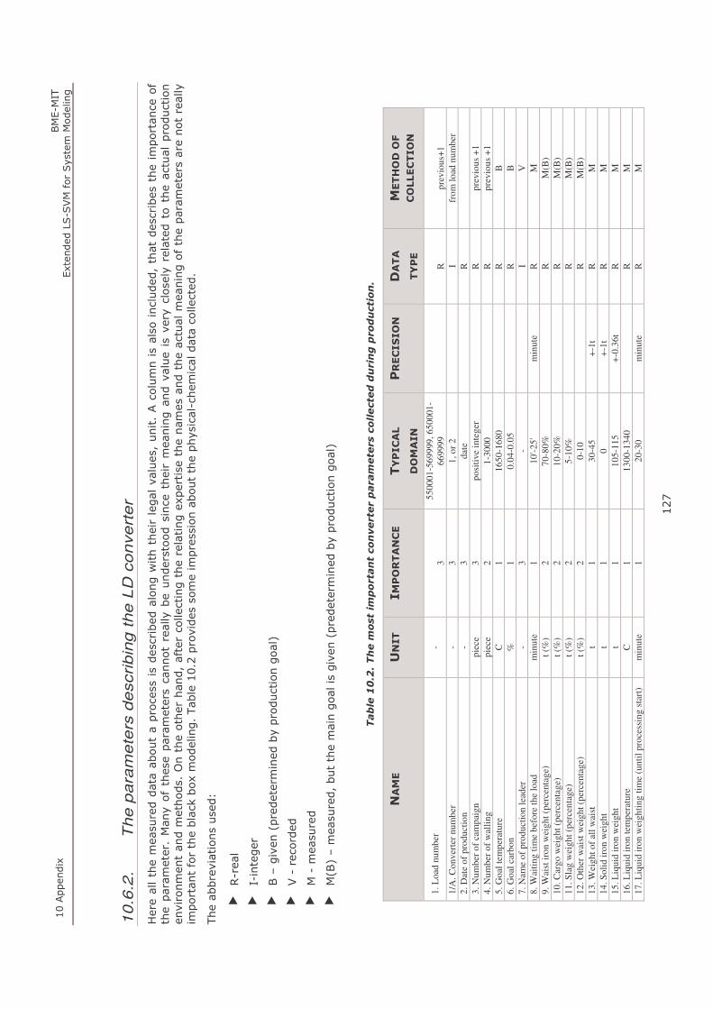
10 Appen
dix
BME-M
IT
Exten
ded
LS-SVM for System M
odeling
127
10
.6.2
. T
he
pa
ram
ete
rs d
escri
bin
g t
he
LD
co
nve
rte
r
Here all the mea
sured data about a process is described
along w
ith their legal values, unit. A column is also included
, that describes the im
portan
ce of
the param
eter. Man
y of these param
eters cannot really be understood since their mea
ning and value is very closely related
to the actual production
environmen
t an
d m
ethods. On the other han
d, after collecting the relating exp
ertise the nam
es and the actual m
eaning of the param
eters are not really
importan
t for the black box modeling. Tab
le 10.2 provides some im
pression about the physical-chem
ical data collected
.
The ab
breviations used:
R-rea
l
I-integer
B – given
(predetermined
by production goal)
V - recorded
M - m
easured
M(B) – m
easured, but the main goal is given
(predetermined
by production goal)
Table 10.2. The m
ost im
porta
nt converte
r paramete
rs collecte
d during production.
NAME
UNIT
IMPORTANCE
TYPICAL
DOMAIN
PRECISION
DATA
TYPE
METHOD OF
COLLECTION
1. L
oad
nu
mb
er
- 3
55
000
1-5
69
999
, 6
50
001
-
66
999
9
R
p
rev
iou
s+1
1/A
. C
on
ver
ter
nu
mb
er
- 3
1
, o
r 2
I fr
om
lo
ad n
um
ber
2. D
ate
of
pro
du
ctio
n
- 3
d
ate
R
3. N
um
ber
of
cam
pai
gn
pie
ce
3
po
siti
ve
inte
ger
R
pre
vio
us
+1
4. N
um
ber
of
wal
lin
g
pie
ce
2
1-3
00
0
R
p
rev
iou
s +
1
5. G
oal
tem
per
atu
re
C
1
16
50
-16
80
R
B
6. G
oal
car
bo
n
%
1
0.0
4-0
.05
R
B
7. N
ame
of
pro
du
ctio
n l
ead
er
- 3
-
I
V
8. W
aiti
ng
tim
e b
efo
re t
he
load
m
inu
te
1
10
'-2
5'
min
ute
R
M
9. W
aist
iro
n w
eig
ht
(per
cen
tag
e)
t (%
) 2
7
0-8
0%
R
M(B
)
10
. C
arg
o w
eig
ht
(per
cen
tag
e)
t (%
) 2
1
0-2
0%
R
M(B
)
11
. S
lag
wei
gh
t (p
erce
nta
ge)
t
(%)
2
5-1
0%
R
M(B
)
12
. O
ther
wai
st w
eig
ht
(per
cen
tag
e)
t (%
) 2
0
-10
R
M
(B)
13
. W
eig
ht
of
all
wai
st
t 1
3
0-4
5
+-1
t R
M
14
. S
oli
d i
ron
wei
gh
t t
1
0
+-1
t R
M
15
. L
iqu
id i
ron
wei
gh
t t
1
10
5-1
15
+-0
.36
t R
M
16
. L
iqu
id i
ron
tem
per
atu
re
C
1
13
00
-13
40
R
M
17
. L
iqu
id i
ron
wei
gh
tin
g t
ime
(un
til
pro
cess
ing
sta
rt)
min
ute
1
2
0-3
0
min
ute
R
M

10 Appen
dix
BME-M
IT
Exten
ded
LS-SVM for System M
odeling
128
NAME
UNIT
IMPORTANCE
TYPICAL
DOMAIN
PRECISION
DATA
TYPE
METHOD OF
COLLECTION
18
. L
iqu
id i
ron
co
mp
osi
tio
n:
C
%
1
4
-4.5
2
%
R
M
Si
%
1
0.6
-1.0
2
%
R
M
Mn
%
2
0
.4-0
.8
1%
R
M
P
%
3
0.0
5-0
.08
4%
R
M
S
%
3
0.0
15
-0.0
30
10
%
R
M
19
. S
lag
cle
anin
g (
yes
/no
) -
3
-
B
V
20
. C
aO a
dd
ed i
n t
he
firs
t 5
min
ute
s o
f th
e m
ain
blo
w
kg
1
60
00
-90
00
+-5
0
R
M
21
. C
aO a
dd
ed d
uri
ng
th
e m
ain
blo
w
kg
2
60
00
-90
00
+-5
0
R
M
22
. C
aF2
ad
ded
in
th
e fi
rst
5 m
inu
tes
of
the
mai
n b
low
k
g
3
15
0-2
50
+-1
0
R
M
23
. C
aF2
ad
ded
duri
ng
th
e m
ain
blo
w
kg
3
15
0-2
50
+-1
0
R
M
24
LD
sla
g a
dd
ed d
uri
ng
th
e m
ain
blo
w
kg
3
0
+-1
0
R
M
25
. O
xyg
en a
dd
ed d
uri
ng
th
e m
ain
blo
w
m3
1
7
50
0-8
50
0
R
M
26
Ar
add
ed d
uri
ng
th
e m
ain
blo
w
m3
3
ab
ou
t 1
0,o
r 0
R
M
27
N2
ad
ded
du
ring
th
e m
ain
blo
w
m3
3
ab
ou
t 2
5, o
r 0
R
M
28
. T
emp
erat
ure
at
the
end
of
the
mai
n b
low
C
1
1
65
0-1
69
0
R
M
29
. T
ime
du
rati
on
bef
ore
tem
per
atu
re m
easu
rem
ent
min
ute
3
3
-5'
min
ute
R
M
30
. T
este
d c
om
po
siti
on
at
the
end
of
mai
n b
low
:
C
%
1
0
.03
-0.0
5
10
%
R
M
Mn
%
3
0
.10
-0.2
5
3%
R
M
S
%
3
0.0
15
-0.0
25
10
%
R
M
P
%
3
0.0
10
-0.0
20
10
%
R
M
31
. S
lag
at
the
end
of
blo
w:
S
iO2
%
3
1
5-2
0
5%
R
M
CaO
%
3
4
8-5
2
3%
R
M
FeO
%
2
1
5-2
5
4%
R
M
Mg
O
%
3
1-2
%
8%
R
M
Mn
O
%
3
4-7
%
? R
M
Al2
O3
%
3
2
-3%
1
0%
R
M
szu
mm
a S
%
3
0
.07
-0.1
?
R
M
P2
O5
%
3
1
-1.2
5%
?
R
M
Baz
icit
y
- 2
2
.6-2
.9
R
M
32
. T
app
ed s
teel
wei
gh
t t
2
12
9-1
35
R
M
(B)
33
. E
nv
iro
nm
ent
tem
per
atu
re
C
1
-10
+3
0
R
N
OT
AV
AIL
AB
LE
34
. C
aO C
O2
co
nte
nt
%
3
R
M(B
)
35
. C
aO 2
min
ute
rea
ctiv
ity
( s
ame
as C
O2
) m
l 3
R
M
(B)

11 References
129
11. REFERENCES
[1] Altrichter Márta, Horváth Gábor, Pataki Béla, Strausz György, Takács Gábor, Valyon József, „Neurális hálózatok”, Panem, 2007.
[2] J. Sjöberg, Q. Zhang, L. Ljung, A. Benveniste, B. Delyon, P.Y. Glorennec, H. Hjalmarsson, A. Juditsky, “Non linear black box modeling in system identification: an unified overview”, Automatica 33, pp. 1691 –1724, 1997.
[3] V. Vapnik, "The Nature of Statistical Learning Theory", New–York: Springer–Verlag., 1995.
[4] V. Vapnik, “Statistical Learning Theory”, John Wiley, NY, 1998.
[5] V. Vapnik, “An overview of statistical learning theory”, IEEE transactions on Neural Networks, Vol. 10(5), pp. 988-1000, 1999.
[6] K. Hornik and M. Stinchcombe, H. White, "Multilayer Feedforward Networks are Universal Approximators", Neural Networks, Vol. 2., pp. 359-366., 1989.
[7] G. Cybenko, "Approximation by Superpositions of a Sigmoidal Function" Mathematics of Control, Signals and Systems, Vol. 3. pp. 303-314, 1989.
[8] J. Park and I. W. Sandberg, "Approximation and Radial-Basis-Function Networks", Neural Computation, 5(2): 305-316., 1993.
[9] N. Cristianini and J. Shawe-Taylor, “An Introduction to Support Vector Machines (and other kernel-based learning methods)”, Cambridge University Press, Cambridge, U.K., 2000.
[10] S. Haykin, "Neural networks. A comprehensive foundation", Prentice Hall, N. J., 1999.
[11] J. A. K. Suykens and J. Vandewalle, “Least squares support vector machine classifiers”, Neural Processing Letters, Vol. 9 (3):293-300, 1999.
[12] J. A. K. Suykens, “Nonlinear Modeling and Support Vector Machines”, IEEE Instrumentation and Measurement Technology Conference, Budapest, Hungary. 2001.
[13] J. A. K. Suykens, V. T. Gestel, J. De Brabanter, B. De Moor, J. Vandewalle, “Least Squares Support Vector Machines”, World Scientific, 2002.
[14] T. Van Gestel, J. A. K. Suykens, B. Baesens, S Viaene, J. Vanthienen, G. Dedene, B. De Moor, and J. Vandewalle, “Benchmarking least squares support vector machine classifiers”, Machine Learning, 2002.
[15] J. A. K. Suykens, L. Lukas, P. Van Dooren, B. De Moor, and J. Vandewalle, “Least squares support vector machine classifiers : a large scale algorithm”, In Proceedings of the European Conference on Circuit Theory and Design (ECCTD-99), pages 839–842, Stresa, Italy, September 1999.
[16] G. C. Cawley, N. L. C. Talbot, “A Greedy Training Algorithm for Sparse Least-Squares Support Vector Machines”, ICANN, pp: 681-686, 2002
[17] W. Chu, C. J. Ong and S.S. Keerthi, “An Improved Conjugate Gradient Scheme to the Solution of Least Squares SVM”, IEEE Transactions on Neural Networks, 16(2), pp. 498-501, 2003.
[18] K. S. Chua, “Efficient computations for large least square support vector machine classifiers”, Pattern Recognition Letters, Vol. 24, 1-3 ,pp. 75 - 80, 2003.
[19] S. S. Keerthi, S. K. Shevade, “SMO algorithm for least-squares SVM formulations”, Neural Computation, Vol. 15 (2), pp. 487 – 507, 2003.

11 References Extended LS
130
[20] B. Hamers, J.A.K. Suykens, B. De Moor, “A comparison of iterative methods for least squares support vector machine classifiers”, Internal Report 01-110, ESAT-SISTA, K.U.Leuven (Leuven, Belgium), 2001.
[21] F. Girosi, “An equivalence between sparse approximation and support vector machines,” Neural Computation, 10 (6),1455–1480, 1998.
[22] J. A. K. Suykens, L. Lukas, and J. Vandewalle, “Sparse least squares support vector machine classifiers”, ESANN'2000 European Symposium on Artificial Neural Networks, pp. 37–42. 2000.
[23] J. A. K. Suykens, L. Lukas, and J. Vandewalle, “Sparse approximation using least squares support vector machines”, IEEE International Symposium on Circuits and Systems ISCAS'2000, 2000.
[24] L. Hoegaerts, J.A.K. Suykens, J. Vandewalle and B. De Moor, “A Comparison of Pruning Algorithms for Sparse Least Squares Support Vector Machines”, Book Lecture Notes in Computer Science, ISBN 978-3-540-23931-4, Springer Berlin / Heidelberg, Volume 3316/2004, pp. 1247-1253, 2004.
[25] B. J. de Kruif and T. J. A. de Vries, “Pruning error minimization in least squares support vector machines,” IEEE Transactions on Neural Networks, vol. 14, no. 3, pp. 696–702, 2003.
[26] R. Reed, “Pruning algorithms – a survey,” IEEE Transactions on Neural Networks, Vol. 4, no. 5, pp. 740–747, 1993.
[27] J. A. K. Suykens, J. De Brabanter, L. Lukas, and J. Vandewalle, “Weighted least squares support vector machines : robustness and sparse approximation”, Neurocomputing, 48(1–4):85–105, 2002.
[28] Gy. Strausz, G. Horváth and B. Pataki: “Effects of database characteristics on the neural modeling of an industrial process” Proc. of the International ICSC/IFAC Symposium on Neural Computation/NC’98, Vienna pp. 834-840, 1998.
[29] R. O. Duda, P. E. Hart and D. G. Stork, “Pattern Classification” (2nd ed.), Wiley Interscience, ISBN: 0-471-05669-3, 2001
[30] C. Bishop, “Improving the generalisation properties of radial basis function neural networks. Neural Computation”, 3(4):579-588, 1991.
[31] J. E. Moody, “The effective number of parameters: An analysis of generalisation and regularisation in nonlinear learning systems” In J.E. Moody, S.J. Hanson, and R.P. Lippmann, editors, Neural Information Processing Systems 4, Morgan Kaufmann, San Mateo CA, pp: 847-854, 1992.
[32] V. S. Cherkassky, F. Mulier, "Learning from Data: Concepts, Theory, and Methods", ISBN:0471154938, John Wiley & Sons Inc., New York, USA, 1998.
[33] B. Schölkopf, and A. Smola. “Learning with Kernels”, MIT Press, Cambridge, MA, 2002.
[34] B. Schölkopf, C. Burges, and A. Smola (eds). “Advances in Kernel Methods - Support Vector Learning”, MIT Press, Cambridge, MA, 1999.
[35] H. Drucker, C. J. C. Burges, L. Kaufman, A. Smola, and V. Vapnik, “Support vector regression machines”, In M. Mozer, M. Jordan, and T. Petsche, editors, Advances in Neural Information Processing Systems 9, pages 155-161, MIT Press, Cambridge, MA, 1997.
[36] C. J. C. Burges. “A Tutorial on Support Vector Machines for Pattern Recognition” Knowledge Discovery and Data Mining, 2(2), 1998.
[37] S. Gunn, “Support Vector Machines for Classification and Regression”, ISIS Technical Report, 1998.
[38] A. J. Smola and B. Schölkopf, “A Tutorial on Support Vector Regression”, NeuroCOLT2 Technical Report Series NC2–TR–1998–030, October, 1998.
[39] E. Osuna, R. Freund, and F. Girosi. “Support vector machines: Training and applications”, Technical Report AIM-1602, MIT A.I. Lab., 1996.
[40] O. Chapelle and V. Vapnik, “Model selection for support vector machines”, In Sara A. Solla, Todd K. Leen, and Klaus-Robert Müller, editors, Advances in Neural Information Processing Systems 12. Cambridge, Mass: MIT Press, 2000.

11 References
131
[41] O. Chapelle, V. Vapnik, O. Bousquet, and S. Mukherjee, “Choosing multiple parameters for support vector machines”, Machine Learning, 2002.
[42] O. Chapelle and V. Vapnik, “Choosing Kernel Parameters for Support Vector Machines”, Machine Learning, 46(1): 131-1569, 2002
[43] O. Chapelle, V. Vapnik and Y. Bengio , “Model Selection for Small Sample Regression”, Machine Learning, 48(1): 9-13, Jul. 2001
[44] N. Cristianini, C. Campbell, and J. Shawe-Taylor. “Dynamically adapting kernels in support vector machines” NeuroCOLT Technical Report NC-TR-98-017, Royal Holloway College, University of London, UK, 1998.
[45] H. Fröhlich, O. Chapelle, B. Schölkopf, “Feature Selection for Support Vector Machines Using Genetic Algorithms”, International Journal on Artificial Intelligence Tools 13(4): 791-800, 2004.
[46] B. E. Boser, I. M. Guyon, V. N. Vapnik, "A training algorithm for optimal margin classifiers", Proceedings of the fifth annual workshop on Computational learning theory, pp. 144 - 152, 1992.
[47] J. Platt, “Fast Training of Support Vector Machines using Sequential Minimal Optimization”, in Advances in Kernel Methods - Support Vector Learning, B. Schölkopf, C. Burges, and A. Smola, eds., MIT Press, 1998.
[48] J. C. Platt, “Sequential Minimal Optimization: Fast Algorithm for Training Support Vector Machines”, Microsoft Research Technical Report MSR–TR–98–14, April 21, 1998.
[49] O. L. Mangasarian and D. R. Musicant, “Successive overrelaxation for support vector machines”, IEEE Transactions on Neural Networks, Vol 10, pp. 1032-1037, 1999.
[50] C. J. C. Burges and B. Schölkopf, “Improving speed and accuracy of support vector learning machines”, In Advances in Neural Information Processing Systems, Vol. 9, pages 375–381. MIT Press, 1997.
[51] E. Osuna, R. Freund, and F. Girosi. “An improved training algorithm for support vector machines” In J. Principe, L. Gile, N. Morgan, and E. Wilson, editors, Neural Networks for Signal Processing VII - roceedings of the 1997 IEEE Workshop, pages 276–285, New York, 1997.
[52] P. Laskov. “An improved decomposition algorithm for regression support vector machines” In S.A. Solla, T.K. Leen, and K.-R. Müller, editors, Advances in Neural Information Processing Systems 12, pp. 484–490. MIT Press, 2000.
[53] S. S. Keerthi, S. K. Shevade, C. Bhattacharyya, and K. R. K. Murthy. “Improvements to Platt's SMO algorithm for SVM classifier design”, Neural Computation Vol. 13, pp. 637-649, March 2001.
[54] S. K. Shevade, S. S. Keerthi, C. Bhattacharyya, and K. R. K. Murthy. “Improvements to the SMO algorithm for regression”, IEEE Transactions on Neural Networks, 11(5):1188-1194, 2000
[55] T. Joachims, “Making Large–Scale SVM Learning Practical”, Advances in Kernel Methods–Support Vector Learning’, MIT Press, Cambridge, USA, 1998.
[56] M. Moser, M. Jordan, & T. Petsche, eds., “Improving the Accuracy and Speed Support Vector Machines”, Neural InformationProcessing Systems Vol. 9., MIT Press, Cambridge, MA, 1997.
[57] E. Osuna and F. Girosi, “Reducing run-time complexity in SVMs”, In Proceedings of the 14th International Conf. on Pattern Recognition, Brisbane, Australia, 1998.
[58] O. L. Mangasarian, “Generalized support vector machines”, Technical Report 98-14, University of Wisconsin, Computer Sciences Department, Madison, WI, USA, Madison, 1998.
[59] Y. J. Lee and O. L. Mangasarian, “SSVM: A smooth support vector machine for classification”, Technical Report 99-03, University of Wisconsin, Data Mining Institute, Madison, 1999.
[60] Y. J. Lee and O. L. Mangasarian, “RSVM: Reduced Support Vector Machines”, Proceedings of the First SIAM International Conference on Data Mining, Chicago, 2001.

11 References Extended LS
132
[61] A.N. Tikhonov and V.Y. Arsenin, “Solutions of Ill-Posed Problems”, Winston, Washington, 1977.
[62] A. E. Hoerl and R. W. Kennard, “Ridge regression: Biased estimation for nonorthogonal problems”, Technometrics, 12(3):55-67, 1970.
[63] Gavin C. Cawley, Nicola L. C. Talbot, “Reduced Rank Kernel Ridge Regression”, Neural Processing Letters 16(3): 293-302, 2002.
[64] C. Saunders, A. Gammerman, V. Vovk, “Ridge Regression Learning Algorithm in Dual Variables”, Proc. 15th International Conf. on Machine Learning, 1998.
[65] M. Espinoza, J. A. K. Suykens and B. D. Moor, "Fixed-size Least Squares Support Vector Machines: A Large Scale Application in Electrical Load Forecasting", Computational Management Science, Springer, Vol. 3(2), pp. 113-129, 2006.
[66] “Numerical Recipes”, Cambridge University Press, Books On-Line, Web: www.nr.com
[67] W. H. Press, S. A. Teukolsky, W. T. Vetterling, and B. P. Flannery, “Numerical Recipes in C : The Art of Scientific Computing”, Cambridge University Press, Cambridge, UK, second edition, 1992.
[68] T. H. Cormen, C. E. Leiserson, R. L. Rivest, C. Stein, "Új algoritmusok", Scolar Kiadó, Budapest, 2003.
[69] G. H. Golub and C. F. Van Loan, “Matrix Computations”, Gene Johns Hopkins University Press, 1989.
[70] S. Mika, G. Rätsch, B. Schölkopf, A. Smola, J. Weston, and K.-R. Müller. „Invariant feature extraction and classification in kernel spaces”. In Advances in Neural Information Processing Systems 12, MIT Press, Cambridge, MA, 1999.
[71] S. Mika, B. Schölkopf, A. Smola, K.-R. Müller, M. Scholz, and G. Rätsch. „Kernel PCA and de-noising in feature spaces”. In M. S. Kearns, S. A. Solla, and D. A. Cohn, editors, Advances in Neural Information Processing Systems 11, MIT Press, pp. 536–542, Cambridge, MA, 1999.
[72] B. Schölkopf, S. Mika, C.J.C. Burges, P. Knirsch, K.-R. Müller, G. Rätsch, and A. Smola. „Input space vs. feature space in kernel-based methods”. IEEE Transactions on Neural Networks, 10(5):1000–1017, 1999.
[73] B. Scholkopf, A. Smola, and K. R. Muller. "Support Vector Methods in Learning and Feature Extraction." Australian Journal of Intelligent Information Processing Systems, Vol. 1, pp. 3-9, 1998.
[74] G. Baudat and F. Anouar, “Kernel-based methods and function approximation”, In Proc. IJCNN, pages 1244–1249, Washington, DC, July 2001.
[75] G. C. Cawley and N. L. C. Talbot, “Efficient formation of a basis in a kernel induced feature space”, In Proceedings of the European Symposium on Artificial Neural Networks (ESANN-2002), pages 1–6, Bruges, Belgium, April 24–26. 2002.
[76] “Matlab 5.3”, Users guide, MathWorks Inc.
[77] P. Cizek, "Asymptotics of least trimmed squares regression", Discussion Paper 72, Tilburg University, Center for Economic Research. , 2004.
[78] P. W. Holland, and R. E. Welsch, "Robust Regression Using Iteratively Reweighted Least-Squares", Communications in Statistics: Theory and Methods, A6, pp. 813-827 , 1977
[79] P. J. Huber, “Robust Statistics”, Wiley, 1981.
[80] J. Van Gorp, J. Schoukens, and R. Pintelon, “Learning neural networks with noisy inputs using, the errors-in-variables approach”, IEEE Transaction on Neural Networks, Vol. 11. No. 2. pp. 402-414. 2000.
[81] C. Blake and C. Merz, “UCI repository of machine learning databases,” [Online]. Available: http://www.ics.uci.edu/~mlearn/MLRepository.html, 1998.
[82] B. Schölkopf and A. J. Smola. “Learning with kernels. Support Vector Machines, Regularisation, Optimisation and Beyond” MIT Press, 2002.
[83] S. Boyd, L. Vandenberghe, “Convex Optimization”, Cambridge University Press, 2004.
11 References
133
[84] G. Horváth, B. Pataki, and Gy. Strausz: "Black box modeling of a complex industrial process", Proc. of the 1999 IEEE Conference and Workshop on Engineering of Computer Based Systems, Nashville, TN, USA., pp. 60-66, 1999.
[85] B. Pataki, G. Horváth, Gy. Strausz, Zs. Talata, "Inverse Neural Modeling of a Linz-Donawitz Steel Converter" e & i Elektrotechnik und Informationstechnik, Vol. 117(1), pp. 13-17. , 2000.