Exposing the Black Box: Intuitive Representation of ARTMAPNetworks

Joshua New and Jian Huang

Abstract— Interactive learning systems have long been used for directed knowledge discovery, volume segmentation, and transferfunction design. Such systems are traditionally treated as black boxes in which a concise summary of the information encoded isnot readily available, forcing professionals to leverage visualization of system weights. The inability of a user to understand learnedpatterns inhibits the ability to make sense of an agent’s exhibited behavior. In this paper, we present an online learning systembased upon Adaptive Resonance Theory which exhibits several practical strengths over traditional learning systems as well as a newmechanism to translate trained networks into intuitive compound boolean range queries. These queries can subsequently be used incombination with parallel coordinate plots to facilitate sense-making of the learned multivariate patterns. We showcase the efficacyof the system by demonstrating it on multivariate jet combustion data as well as tumor segmentation from MRI.

Index Terms—Learning systems, compound boolean range queries, large multivariate data visualization.

F

1 INTRODUCTION

As the size of modern datasets continues to grow, the problems ofknowledge discovery, feature specification and tracking, as well as hy-pothesis testing becomes increasingly intractable. Fully automated fil-tering and computational tools are useful to aid in the process, butcan rarely be used holistically within a given domain-specific context.Indeed, visualization rests upon the assumption that no matter howgood pattern recognition and automation is, the best it can be is semi-automatic within the context of the entire scientific process; there is nomagic to jump from fuzzy concepts to fully substantiated and verifi-able specifications. In this paper, we seek to leverage visualization andcognitive processing to train the computer which patterns are deemedinteresting. Furthermore, we seek to translate a traditionally blackbox learning system into a series of intuitive representations that canbe then be used to facilitate understanding and promote scientific ad-vances.

There are a wealth of learning systems which have been used withinthe visualization community for everything from autonomous patterndetection to transfer function design. While every system has its ownstrengths and weaknesses, we have elected to use a fuzzy learningsystem based upon Adaptive Resonance Theory (ART) due to sev-eral technical strengths and few weaknesses outlined in Section 3.2.ART is a mathematical model designed to address the “stability-plasticity” dilemma in which learning systems must be stable enoughto avoid castastrophic forgetting but plastic enough to continuouslylearn. ART-based learning systems accomplish this by growing in sizeas new experiences are introduced but also retains perfect memory ofpast experiences. In this paper, we present an interactive segmenta-tion system in which a user can succesively refine segmentation re-sults from a heterogeneous network of learning systems using intuitivebrushing of interesting image locations.

While codifying human knowledge into autonomous agents can bevery useful, it has often been the case that extracting learned knowl-edge from an agent has been notoriously difficult. ART-based systems,like most learning systems, are often treated as black boxes in whichthe learned properties are encoded in a nearly-indecipherable series ofedge weights. Several attempts have been made at visualizing neuralnets in order to comprehend the reasons for exhibited behavior. In thispaper, we present a method for converting SFAM networks into a rep-resentation as compound boolean range queries which can be used to

• All authors are with the Department of Electrical Engineering andComputer Science of the University of Tennessee, Knoxville. Email: {new,huangj}@cs.utk.edu.

Manuscript received 30 July 2007.Under review.

intuitively and precisely identify learned categories and also presentedin the context of multivariate relationships using parallel coordinateplots.

In the remainder of this paper, we first give a summary of relatedworks in Section 2. In Section 3 we introduce the technical details ofour contributions. Finally, our results and discussion are provided inSection 4, and then concluded in Section 5.

2 BACKGROUND

2.1 Segmentation with Learning Systems

Segmentation is defined as the act or process of dividing into seg-ments. In image segmentation, there is a feature vector per pixel lo-cation which contains multiple features corresponding to the valuesfor each of the variables available for that pixel location. Volume seg-mentation can effectively be extruded from image segmentation overmultiple slices.

Machine learning is defined as the ability of a machine to improveits performance based on previous results. Machine learning sys-tems allow automatic segmentation through “clustering” feature vec-tors into categories/classes. Machine learning systems come in threeflavors; in increasing order of capability they are unsupervised, rein-forced, and supervised. An unsupervised system is provided no hinttothe correct classification, a reinforced system is provided a good/badhint to the correct classification, and a supervised system is given thecorrect answer.

There are several common techniques and problems with segment-ing data. Segmentation techniques can be broken into two generalcategories: manual, semi-automatic, and automatic. In manual seg-mentation, users must draw the desired borders onto the raw im-age. While manual segmentation is often highly accurate, this processtakes much time, can be highly fatiguing, prone to errors, and ob-fuscate reproducibility. Automatic segmentation promises to addressmany of these issues. A short list of automatic segmentation meth-ods includes Active Shape/Contour Models, Adaptive Segmentation,Bayesian Grouping, probabilistic neural networks, and Fuzzy cluster-ing techniques. An analysis of these automatic segmentation meth-ods and related problems is beyond the scope of this work, but theinterested reader is referred to [6] showcased in the domain of brainsegmentation from MRI. All known automatic segmentation methodssuffer in varying degrees from problems such as variable imaging orsimulation parameters, signal noise, overlapping intensities for contin-uous data points mapping to an implicit grid, partial voluming effects,gradients from discontinuities between successive slices or timesteps,and many other domain-specific concerns exist which make segmen-tation a “confidence”-related task. For this reason, semi-automaticmethods are often used in which a human expert can leverage com-

putational tools to negotiate the tradeoffs between conflicting effectsto mark up data with a much-reduced workload over a fully manualsegmentation.

2.2 Adaptive Resonance Theory

Adaptive Resonance Theory (ART) is a mathematical frameworkbased upon models of the hippocampus and neocortex developed byCarpenter and Grossberg in the 70s [7]. Many connectionist networksat the time suffered from the Stability-Plasticity Dilemma, whichstates the trade-off between a learning system stable enough to pre-serve learned patterns and yet plastic enough to learn new ones [8].Adaptive Resonance Theory was developed to overcome this dilemmaand has since served as a host for a plethora of neural network archi-tectures, each demonstrating varying capabilities.

The ART1 class of architectures, developed in 1983, establishedthe first ART-based neural network and performs unsupervised learn-ing for binary input patterns [4]. The ART2 class of architectures,developed in 1987, included the ability to recognize analog vectors inwhich features are codified to a floating point between 0 and 1 [2].ART3 [3] and ARTMAP [5], developed ART3 and ARTMAP, devel-oped in 1987 and 1991 respectively, are members of the ART2 class ofarchitectures along with dozens of other modern variants. The ART2architecture variant known as Simplified Fuzzy ARTMAP is the onethat was utilized in this study due to its computational efficiency, in-teractive performance, and many other properties that will be detailedlater.

Simplified Fuzzy ARTMAP (SFAM) [12] is a fast, on-line/interactive, incremental, supervised learning system for analogsignals. Fuzzy means that SFAM utilizes fuzzy learning rules for ac-tivation and selection of simulated neurons. SFAM can learn at a cus-tom rate, but the fast learning rule is used because the simple fuzzylearning rules minimize the computation required for learning. SFAMis essentially a two-layer neural network that is specialized for patternrecognition, capable of learning every training pattern with very fewiterations. The network starts with no connection weights, grows insize to suit the problem, uses simple learning equations, and has onlyone user-selectable parameter. In this system, the input vectors corre-spond to multiple metrics which defines the relationship for each pairof attributes from a set of multivariate data. SFAM is particularly wellsuited to this problem and we circumvent the dependence on an ad-justable “vigilance” parameter and the dependence on the order of theinput by using a voting scheme of heterogeneous networks.

3 SYSTEM COMPONENTS

As the resolution and number of variables increases in modern multi-variate datasets, the ability to precisely identify interesting patterns inthe dataset becomes increasingly intractable. This is exacerbated bythe fact that one could compute a large number of derivative variables.Human cognitive ability could be overloaded in regard to remember-ing and using various combinations of metrics for a plethora of rele-vant scenarios. As is common with initial investigation of new data,experts may not even know what is important until they see it.

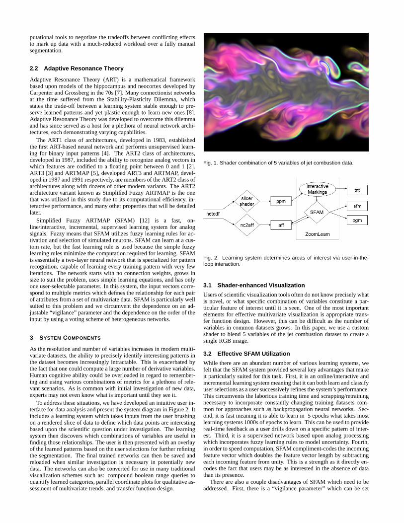
To address these situations, we have developed an intuitive user in-terface for data analysis and present the system diagram in Figure 2. Itincludes a learning system which takes inputs from the user brushingon a rendered slice of data to define which data points are interestingbased upon the scientific question under investigation. The learningsystem then discovers which combinations of variables are useful infinding those relationships. The user is then presented with an overlayof the learned patterns based on the user selections for further refiningthe segmentation. The final trained networks can then be saved andreloaded when similar investigation is necessary in potentially newdata. The networks can also be converted for use in many traditionalvisualization schemes such as: compound boolean range queries toquantify learned categories, parallel coordinate plots for qualitative as-sessment of multivariate trends, and transfer function design.

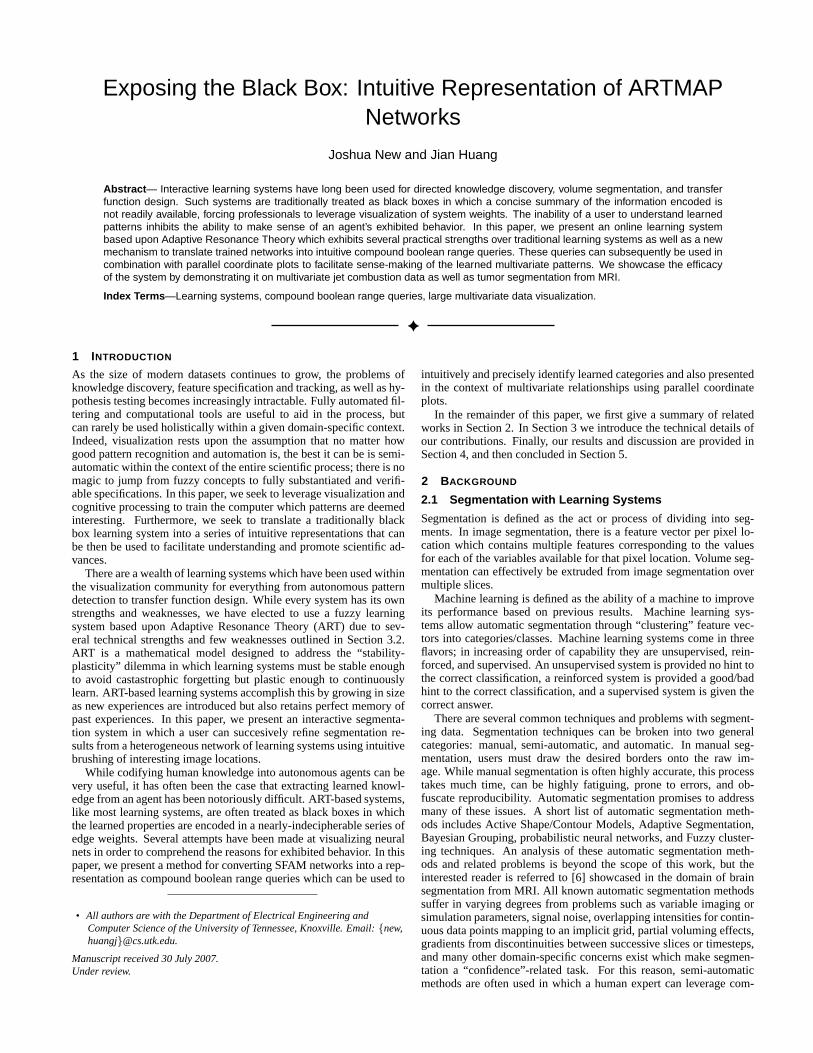
Fig. 1. Shader combination of 5 variables of jet combustion data.

Fig. 2. Learning system determines areas of interest via user-in-the-loop interaction.

3.1 Shader-enhanced Visualization

Users of scientific visualization tools often do not know precisely whatis novel, or what specific combination of variables constitute a par-ticular feature of interest until it is seen. One of the most importantelements for effective multivariate visualization is appropriate trans-fer function design. However, this can be difficult as the number ofvariables in common datasets grows. In this paper, we use a customshader to blend 5 variables of the jet combustion dataset to create asingle RGB image.

3.2 Effective SFAM Utilization

While there are an abundant number of various learning systems, wefelt that the SFAM system provided several key advantages that makeit particularly suited for this task. First, it is an online/interactive andincremental learning system meaning that it can both learn and classifyuser selections as a user successively refines the system’s performance.This circumvents the laborious training time and scrapping/retrainingnecessary to incorporate constantly changing training datasets com-mon for approaches such as backpropagation neural networks. Sec-ond, it is fast meaning it is able to learn in 5 epochs what takes mostlearning systems 1000s of epochs to learn. This can be used to providereal-time feedback as a user drills down on a specific pattern of inter-est. Third, it is a supervised network based upon analog processingwhich incorporates fuzzy learning rules to model uncertainty. Fourth,in order to speed computation, SFAM compliment-codes the incomingfeature vector which doubles the feature vector length by subtractingeach incoming feature from unity. This is a strength as it directly en-codes the fact that users may be as interested in the absence of datathan its presence.

There are also a couple disadvantages of SFAM which need to beaddressed. First, there is a “vigilance parameter” which can be set

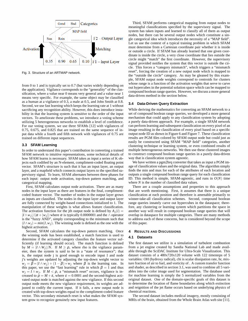
Fig. 3. Structure of an ARTMAP network.

from 0 to 1 and is typically set to 0.7 (but varies widely depending onthe application). Vigilance corresponds to the “generality” of the clas-sification, where a value near 0 means very general and a value near 1means very specific. For example, the same object may be classifiedas a human at a vigilance of 0.3, a male at 0.5, and John Smith at 0.8.Second, we use fast learning which keeps the learning rate at 1 withoutsacrificing any recognition ability. However, this does introduce insta-bility in that the learning system is sensitive to the order of the inputvectors. To ameliorate these problems, we introduce a voting schemeutilizing 5 heterogeneous networks to establish a level of confidence.For our voting system, we use three SFAMs [12] with vigilances of0.75, 0.675, and 0.825 that are trained on the same sequence of in-put data while a fourth and fifth network with vigilances of 0.75 aretrained on different input sequences.

3.3 SFAM LearningIn order to understand this paper’s contribution in converting a trainedSFAM network to intuitive representations, some technical details ofhow SFAM learns is necessary. SFAM takes as input a series of K ob-jects each codified by an N-element, compliment-coded floating pointvector. SFAM’s structure is such that it has an input layer, an outputlayer, and a mapfield which connects output layers to the specified su-pervisory signal. To learn, SFAM alternates between three phases foreach input: output node activation, top-down pattern matching, andcategorical mapping.

First, SFAM calculates output node activation. There are as manynodes in the input layer as there are features in the final, compliment-coded feature vector. The number of nodes in the output layer growsas inputs are classified. The nodes in the input layer and output layerare fully connected by weight-based connections initialized to 1. Themanipulation of these weights is what allows feature classification.The activation function for the jth output node is defined byA j (i) =|I ∧w j |/(α + |w j |) whereα is typically 0.0000001 and the∧ operatoris the “fuzzy AND”, simply corresponding to the minimum such that(I ∧w j ) = min(I ,w j). The winning node is defined as the one with thehighest activation.

Second, SFAM calculates the top-down pattern matching. Oncethe winning node has been established, a match function is used todetermine if the activated category classifies the feature vector suf-ficiently (if learning should occur). The match function is definedby M = |I ∧Wj |/N. If M ≥ ρ , where rho is the vigilance param-eter, then the system is said to be in a “state of resonance”; thatis, the output node j is good enough to encode input I and nodej’s weights are updated by adjusting the top-down weight vector tow j = β ∗ (I ∧ w j ) + (1− β ) ∗ w j where β is the learning rate. Inthis paper, we use the “fast learning” rule in whichβ = 1 and thusw j = I ∧w j . If M < ρ , a “mismatch reset” occurs, vigilance is in-creased toρ = M + ε, whereε = 0.0001 and the second-highest acti-vated output node is matched against the new vigilance. If this secondoutput node meets the new vigilance requirement, its weights are ad-justed to codify the current input. If it fails, a new output node iscreated with top-down weights equal to the compliment-coded featurevector. This secondary mismatch reset is what makes the SFAM sys-tem grow to recognize genuinely new input features.

Third, SFAM performs categorical mapping from output nodes tomeaningful classifications specified by the supervisory signal. Thesystem has taken inputs and learned to classify all of them as outputnodes, but there can be several output nodes which constitute a sin-gle categorical idea which introduces the necessity of a “MAP field”.Let us use the context of a typical training problem in which SFAMmust determine from a Cartesian coordinate pair whether it is insideor outside a circle. If SFAM has already learned that one given coor-dinate is inside the circle, a very close coordinate that lies outside thecircle might “match” the first coordinate. However, the supervisorysignal provided notifies the system that this vector is outside the cir-cle. This forces a “category mismatch”, which triggers a “mismatchreset”, forcing the creation of a new output node which is mapped tothe “outside the circle” category. As may be gleaned by this exam-ple, SFAM output node weights correspond to centroids for clusterswhose range is a function of the activation weights that serve to carveout hypercubes in the potential solution space which can be mapped tocompound boolean range queries. However, we discuss a more generaldata-driven method in the section below.

3.4 Data-Driven Query Extraction

While deriving the mathematics for converting an SFAM network to aset of compound boolean range queries, we developed a more generalmechanism that could apply to any classification system by adoptinga purely data-driven approach. For example, a single SFAM networkcan perform learning and subsequent classification on every pixel ofanimage resulting in the classification of every pixel based on a specificoutput node ID as shown in Figure 6 and Figure 7. These classificationresults are PGM files colored by SFAM output node but could just aseasily be constructed using SFAM “MAP field” categories, anotherclustering technique or learning system, or even combined results ofmultiple heterogeneous networks. We then use these clustered imagesto construct compound boolean range queries in a purely data-drivenway that is classification system agnostic.

We have written a pgm2brq converter that takes as input a PGM im-age of classification values and the original data. The algorithm simplyfinds the min and max for each of the attributes of each location andoutputs a single compound boolean range query for each classificationID. This method is simple, SFAM-agnostic, and runs inO(N) timewhereN is the number of classified data values.

There are a couple assumptions and properties to this approachthat are worth mentioning. First, it assumes that there is a uniqueclassification at each position and therefore is amenable primarily towinner-take-all classification schemes. Second, compound booleanrange queries innately carve out hypercubes in the dataspace; there-fore, any clustering or learning system which partitions the space inanother way will result in compound boolean range queries that willoverlap in dataspace for multiple categories. There are many methodsto address each of these concerns, but is considered beyond the scopeof this paper.

4 RESULTS AND DISCUSSIONS

4.1 Datasets

The first dataset we utilize is a simulation of turbulent combustionfrom a jet engine created by Sandia National Lab and made avail-able through the SciDAC Institute for Ultra-Scale Visualization. Thisdataset consists of a 480x720x120 volume with 122 timesteps of 5variables: OH (hydroxy radical), chi is scalar dissipation rate, hr, mix-ture fraction of air to fuel, and vorticity of . A custom transfer functionand shader, as described in section 3.1, was used to combine all 5 vari-ables into the color image used for segmentation. The database usedfor machine learning is simply the 5 normalized variables from theoriginal dataset. One of the domain-specific goals of this dataset isto determine the location of flame boundaries along which extinctionand reignition of the jet flame occurs based on underlying physics ofchemical reactions.

The second dataset includes medical imagery, mostly consisting ofMRIs of the brain, obtained from the Whole Brain Atlas web site [11].

Fig. 4. Segmentation of flame boundaries in the jet combustion dataset.

This dataset consists of 256x256 image slices from the brain of a pa-tient suffering from metastatic bronchogenic carcinoma. To gener-ate the database of information for the SFAM-based segmentation, wetook the spatially registered PD, T1, T2, and SPECT imaging modali-ties and used image processing with the 3D shunt operator [1] to create16 opponency values for each pixel location. A sample of 3 of theseopponencies was used as YIQ channels and then mapped to RGB chro-matic space for display of multiple modalities simultaneously. One ofthe domain-specific goals is to segment the unhealthy brain tissue forplanning of decompressive surgery.

4.2 Segmentation

The segmentation GUI is intuitive to use and capable of robustly delin-eating features in the data with only a few swipes of the mouse. In thisinterface, we use green to denote examples and red to denote coun-terexamples. Based upon these markings, the SFAM networks ana-lyze the database information and report a gray-scale image recordingthe confidence of the heterogeneous collection of learning systems ofother points similar to those selected by the user.

As can be seen in Figure 4, successful segmentation of flame bound-aries is displayed. For this segmentation task, an unusually large num-ber of disjoint points, consisting of 17 examples and 32 counterexam-ples, was utilized in order to highlight the strength of both the SFAMnetworks as well as the subsequent extraction of quantitative queries.Although 49 points were used, the SFAM networks created an averageof only 7 output nodes per network to encode the diffent material typesin the dataset. This results in data reduction and a filtered clustering ofthe dataset to aid in comprehension and attention direction.

Figure 5 showcases successful segmentation of metastatic bron-chogenic carcinoma. This segmentation task involved only 3 swipes ofthe mouse and transparent network training despite 68 training pointsencoded using an average of 40 output nodes over 32 complement-coded features. The heterogeous set of trained agents is saved and cansubsequently be utilized on a database of patients to scan for imageswhich exhibit similar risk of this disease or for use in prescreeningto direct radiologist’s attention to the most likely locations of variousdisease types.

Fig. 5. Segmentation of tumor in MRI dataset.

4.3 Transfer Function Design

Segmentation and other classification schemes can be used to createeffective transfer function designs of structure within the data. In Fig-ure 4 and Figure 5, we simply show a segmentation confidence overlay.This segmentation overlay could instead be used to modulate opacityfor different structures depending on the task at hand. Indeed, assum-ing that the learning system used provides robust segmentation acrossslices, this method could be applied to multiple slices of a volumetricdataset for identification of isosurfaces or interval volumes that couldbe made transparent or highlighted for feature tracking.

In order to learn more about the dataset, we color the datasets byoutput node of an SFAM networks trained to recognize flame bound-aries and carcinoma in Figure 6 and Figure 7. This classificationclearly shows very coherent structures in the data in a method verysimilar to the non-photorealistic technique of toonification. This sametechnique could be applied to SFAM output nodes for material types,SFAM Map field categories to reduce this knowledge down to the seg-mentation results, multiple heterogeneous networks trained for a com-mon task as in Figure 4 and Figure 5, or even multiple clustering orclassification systems trained for different tasks (such as toonified re-sults for various types of diseases visible to multiple image modali-ties).

4.4 Query Representation

While autonomous learning systems are useful in many circumstances,domain scientists are often trying to determine precisely which inter-play of variables is giving rise to a specific, visual effect. In order toopen the black box and allow the user to understand what the systemhas learned, we have developed a data-driven mechanism for mappinga set of classifications to a set of compound boolean range queries. Forthe result in Figure 4, we show the data-space centroid correspondingto each grayscale level in Table 1.

In these 10 complement-coded data centroids from the output nodesof an SFAM network, we have a strong delineation of specific types ofchemical concentrations and their corresponding location within thedataset. There are 2 example classes which codify somewhat similarchemical properties of the flame boundaries. There are 3 counterex-ample nodes in which the first cluster consists only of data points in-side the flame boundaries near the center of the simulation, the second

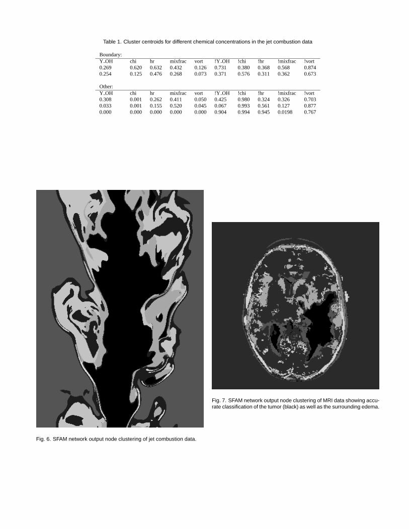
Table 1. Cluster centroids for different chemical concentrations in the jet combustion data

Boundary:Y OH chi hr mixfrac vort !YOH !chi !hr !mixfrac !vort0.269 0.620 0.632 0.432 0.126 0.731 0.380 0.368 0.568 0.8740.254 0.125 0.476 0.268 0.073 0.371 0.576 0.311 0.362 0.673

Other:Y OH chi hr mixfrac vort !YOH !chi !hr !mixfrac !vort0.308 0.001 0.262 0.411 0.050 0.425 0.980 0.324 0.326 0.7030.033 0.001 0.155 0.520 0.045 0.067 0.993 0.561 0.127 0.8770.000 0.000 0.000 0.000 0.000 0.904 0.994 0.945 0.0198 0.767

Fig. 6. SFAM network output node clustering of jet combustion data.

Fig. 7. SFAM network output node clustering of MRI data showing accu-rate classification of the tumor (black) as well as the surrounding edema.

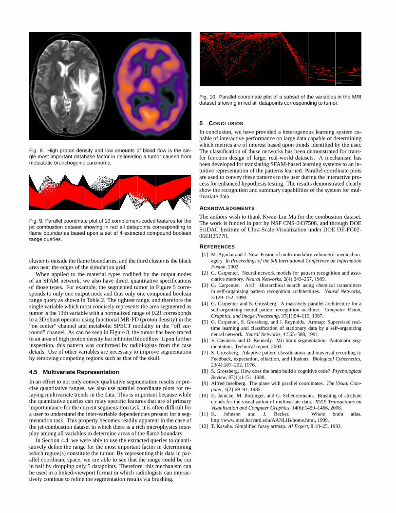
Fig. 8. High proton density and low amounts of blood flow is the sin-gle most important database factor in delineating a tumor caused frommetastatic bronchogenic carcinoma.

Fig. 9. Parallel coordinate plot of 10 complement-coded features for thejet combustion dataset showing in red all datapoints corresponding toflame boundaries based upon a set of 4 extracted compound booleanrange queries.

cluster is outside the flame boundaries, and the third cluster is the blackarea near the edges of the simulation grid.

When applied to the material types codified by the output nodesof an SFAM network, we also have direct quantitative specificationsof those types. For example, the segmented tumor in Figure 5 corre-sponds to only one output node and thus only one compound booleanrange query as shown in Table 2. The tightest range, and therefore thesingle variable which most concisely represents the area segmented astumor is the 13th variable with a normalized range of 0.21 correspondsto a 3D shunt operator using functional MR-PD (proton density) in the“on center” channel and metabolic SPECT modality in the “off sur-round” channel. As can be seen in Figure 8, the tumor has been tracedto an area of high proton density but inhibited bloodflow. Upon furtherinspection, this pattern was confirmed by radiologists from the casedetails. Use of other variables are necessary to improve segmentationby removing competing regions such as that of the skull.

4.5 Multivariate Representation

In an effort to not only convey qualitative segmentation results or pre-cise quantitative ranges, we also use parallel coordinate plots for re-laying multivariate trends in the data. This is important because whilethe quantitative queries can relay specific features that are of primaryimportantance for the current segmentation task, it is often difficult fora user to understand the inter-variable dependencies present for a seg-mentation task. This property becomes readily apparent in the case ofthe jet combustion dataset in which there is a rich microphysics inter-play among all variables to determine areas of the flame boundary.

In Section 4.4, we were able to use the extracted queries to quanti-tatively define the range for the most important factor in determiningwhich region(s) constitute the tumor. By representing this data in par-allel coordinate space, we are able to see that the range could be cutin half by dropping only 5 datapoints. Therefore, this mechanism canbe used in a linked-viewport format in which radiologists can interac-tively continue to refine the segmentation results via brushing.

Fig. 10. Parallel coordinate plot of a subset of the variables in the MRIdataset showing in red all datapoints corresponding to tumor.

5 CONCLUSION

In conclusion, we have provided a heterogenous learning system ca-pable of interactive performance on large data capable of determiningwhich metrics are of interest based upon trends identified by the user.The classification of these networks has been demonstrated for trans-fer function design of large, real-world datasets. A mechanism hasbeen developed for translating SFAM-based learning systems to an in-tuitive representation of the patterns learned. Parallel coordinate plotsare used to convey these patterns to the user during the interactive pro-cess for enhanced hypothesis testing. The results demonstrated clearlyshow the recognition and summary capabilities of the system for mul-tivariate data.

ACKNOWLEDGMENTS

The authors wish to thank Kwan-Liu Ma for the combustion dataset.The work is funded in part by NSF CNS-0437508, and through DOESciDAC Institute of Ultra-Scale Visualization under DOE DE-FC02-06ER25778.

REFERENCES

[1] M. Aguilar and J. New. Fusion of multi-modality volumetric medical im-agery. InProceedings of the 5th Inernational Conference on InformationFusion, 2002.

[2] G. Carpenter. Neural network models for pattern recognition and asso-ciative memory.Neural Networks, 2(4):243–257, 1989.

[3] G. Carpenter. Art3: Hierarchical search using chemical transmittersin self-organizing pattern recognition architectures.Neural Networks,3:129–152, 1990.

[4] G. Carpenter and S. Grossberg. A massively parallel architecture for aself-organizing neural pattern recognition machine.Computer Vision,Graphics, and Image Processing, 37(1):54–115, 1987.

[5] G. Carpenter, S. Grossberg, and J. Reynolds. Artmap: Supervised real-time learning and classification of stationary data by a self-organizingneural network.Neural Networks, 4:565–588, 1991.

[6] V. Caviness and D. Kennedy. Mri brain segmentation: Automatic seg-mentation. Technical report, 2004.

[7] S. Grossberg. Adaptive pattern classification and universal recording ii:Feedback, expectation, olfaction, and illusions.Biological Cybernetics,23(4):187–202, 1976.

[8] S. Grossberg. How does the brain build a cognitive code?PsychologicalReview, 87(1):1–51, 1980.

[9] Alfred Inselberg. The plane with parallel coordinates.The Visual Com-puter, 1(2):69–91, 1985.

[10] H. Janicke, M. Bottinger, and G. Scheurermann. Brushingof attributeclouds for the visualization of multivariate data.IEEE Transactions onVisaulization and Computer Graphics, 14(6):1459–1466, 2008.

[11] K. Johnson and J. Becker. Whole brain atlas.http://www.med.harvard.edu/AANLIB/home.html, 1999.

[12] T. Kasuba. Simplified fuzzy artmap.AI Expert, 8:18–25, 1993.

Table 2. Extracted 32-feature query for tumor in MRI data corresponding to the black region of Figure 8.

[0.245,0.990] [0.100,1.000] [0.405,0.998] [0.000,0.326] [0.114,0.991] [0.145,0.916] [0.560,1.000] [0.161,0.880][0.154,0.505] [0.208,1.000] [0.103,0.998] [0.137,0.992] [0.789,1.000] [0.000,0.405] [0.000,0.376] [0.000,0.358][0.010,0.755] [0.000,0.900] [0.002,0.595] [0.674,1.000] [0.009,0.886] [0.084,0.855] [0.000,0.440] [0.120,0.839][0.495,0.846] [0.000,0.792] [0.002,0.897] [0.008,0.863] [0.000,0.210] [0.595,1.000] [0.624,1.000] [0.642,1.000]