exposing digital forgeries through chromatic aberration
TRANSCRIPT
Exposing Digital Forgeries Through Chromatic Aberration
Micah K. JohnsonDepartment of Computer Science
Dartmouth CollegeHanover, NH 03755
Hany FaridDepartment of Computer Science
Dartmouth CollegeHanover, NH 03755
ABSTRACTVirtually all optical imaging systems introduce a variety ofaberrations into an image. Chromatic aberration, for exam-ple, results from the failure of an optical system to perfectlyfocus light of different wavelengths. Lateral chromatic aber-ration manifests itself, to a first-order approximation, as anexpansion/contraction of color channels with respect to oneanother. When tampering with an image, this aberration isoften disturbed and fails to be consistent across the image.We describe a computational technique for automatically es-timating lateral chromatic aberration and show its efficacyin detecting digital tampering.
Categories and Subject DescriptorsI.4 [Image Processing]: Miscellaneous
General TermsSecurity
KeywordsDigital Tampering, Digital Forensics
1. INTRODUCTIONMost images contain a variety of aberrations that result
from imperfections and artifacts of the optical imaging sys-tem. In an ideal imaging system, light passes through thelens and is focused to a single point on the sensor. Opticalsystems, however, deviate from such ideal models in thatthey fail to perfectly focus light of all wavelengths. Theresulting effect is known as chromatic aberration which oc-curs in two forms: longitudinal and lateral. Longitudinalaberration manifests itself as differences in the focal planesfor different wavelengths of light. Lateral aberration mani-fests itself as a spatial shift in the locations where light ofdifferent wavelengths reach the sensor – this shift is pro-portional to the distance from the optical center. In both
Permission to make digital or hard copies of all or part of this work forpersonal or classroom use is granted without fee provided that copies arenot made or distributed for profit or commercial advantage and that copiesbear this notice and the full citation on the first page. To copy otherwise, torepublish, to post on servers or to redistribute to lists, requires prior specificpermission and/or a fee.MM&Sec’06, September 26–27, 2006, Geneva, Switzerland.Copyright 2006 ACM 1-59593-493-6/06/0009 ...$5.00.
cases, chromatic aberration leads to various forms of colorimperfections in the image. To a first-order approximation,longitudinal aberration can be modeled as a convolution ofthe individual color channels with an appropriate low-passfilter. Lateral aberration, on the other hand, can be mod-eled as an expansion/contraction of the color channels withrespect to one another. When tampering with an image,these aberrations are often disturbed and fail to be consis-tent across the image.
We describe a computational technique for automaticallyestimating lateral chromatic aberration. Although we even-tually plan to incorporate longitudinal chromatic aberra-tion, only lateral chromatic aberration is considered here.We show the efficacy of this approach for detecting digitaltampering in synthetic and real images. This work providesanother tool in a growing number of image forensic tools, [3,7, 8, 10, 9, 5, 6].
2. CHROMATIC ABERRATIONWe describe the cause of lateral chromatic aberration and
derive an expression for modeling it. For purposes of expo-sition a one-dimensional imaging system is first considered,and then the derivations are extended to two dimensions.
2.1 1-D AberrationIn classical optics, the refraction of light at the boundary
between two media is described by Snell’s Law:
n sin(θ) = nf sin(θf ), (1)
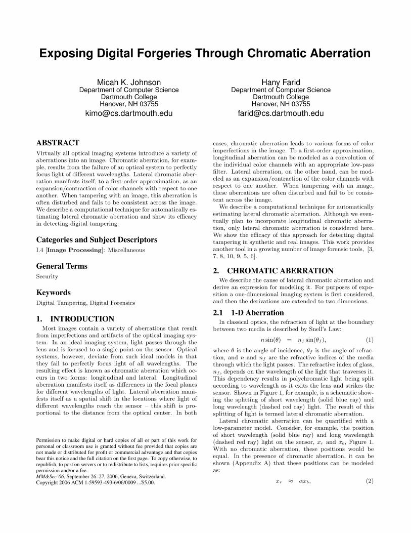
where θ is the angle of incidence, θf is the angle of refrac-tion, and n and nf are the refractive indices of the mediathrough which the light passes. The refractive index of glass,nf , depends on the wavelength of the light that traverses it.This dependency results in polychromatic light being splitaccording to wavelength as it exits the lens and strikes thesensor. Shown in Figure 1, for example, is a schematic show-ing the splitting of short wavelength (solid blue ray) andlong wavelength (dashed red ray) light. The result of thissplitting of light is termed lateral chromatic aberration.
Lateral chromatic aberration can be quantified with alow-parameter model. Consider, for example, the positionof short wavelength (solid blue ray) and long wavelength(dashed red ray) light on the sensor, xr and xb, Figure 1.With no chromatic aberration, these positions would beequal. In the presence of chromatic aberration, it can beshown (Appendix A) that these positions can be modeledas:
xr ≈ αxb, (2)
f
xr
θr
xb
θb
Lens
Sensor
θ
Figure 1: The refraction of light in one dimension.Polychromatic light enters the lens at an angle θ, andemerges at an angle which depends on wavelength.As a result, different wavelengths of light, two ofwhich are represented as the red (dashed) and theblue (solid) rays, will be imaged at different points,xr and xb.
where α is a scalar value. This model generalizes for any twowavelengths of light, where α is a function of these wave-lengths.
2.2 2-D AberrationFor a two-dimensional lens and sensor, the distortion
caused by lateral chromatic aberration takes a form sim-ilar to Equation (2). Consider again the position of shortwavelength (solid blue ray) and long wavelength (dashed redray) light on the sensor, (xr, yr) and (xb, yb). In the pres-ence of chromatic aberration, it can be shown (Appendix A)that these positions can be modeled as:
(xr, yr) ≈ α(xb, yb), (3)
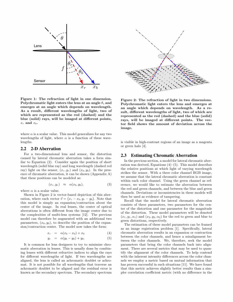
where α is a scalar value.Shown in Figure 2 is vector-based depiction of this aber-
ration, where each vector ~v =`xr − xb, yr − yb
´. Note that
this model is simply an expansion/contraction about thecenter of the image. In real lenses, the center of opticalaberrations is often different from the image center due tothe complexities of multi-lens systems [12]. The previousmodel can therefore be augmented with an additional twoparameters, (x0, y0), to describe the position of the expan-sion/contraction center. The model now takes the form:
xr = α(xb − x0) + x0 (4)
yr = α(yb − y0) + y0. (5)
It is common for lens designers to try to minimize chro-matic aberration in lenses. This is usually done by combin-ing lenses with different refractive indices to align the raysfor different wavelengths of light. If two wavelengths arealigned, the lens is called an achromatic doublet or achro-mat. It is not possible for all wavelengths that traverse anachromatic doublet to be aligned and the residual error isknown as the secondary spectrum. The secondary spectrum
Figure 2: The refraction of light in two dimensions.Polychromatic light enters the lens and emerges atan angle which depends on wavelength. As a re-sult, different wavelengths of light, two of which arerepresented as the red (dashed) and the blue (solid)rays, will be imaged at different points. The vec-tor field shows the amount of deviation across theimage.
is visible in high-contrast regions of an image as a magentaor green halo [4].
2.3 Estimating Chromatic AberrationIn the previous section, a model for lateral chromatic aber-
ration was derived, Equations (4)–(5). This model describesthe relative positions at which light of varying wavelengthstrikes the sensor. With a three color channel RGB image,we assume that the lateral chromatic aberration is constantwithin each color channel. Using the green channel as ref-erence, we would like to estimate the aberration betweenthe red and green channels, and between the blue and greenchannels. Deviations or inconsistencies in these models willthen be used as evidence of tampering.
Recall that the model for lateral chromatic aberrationconsists of three parameters, two parameters for the cen-ter of the distortion and one parameter for the magnitudeof the distortion. These model parameters will be denoted(x1, y1, α1) and (x2, y2, α2) for the red to green and blue togreen distortions, respectively.
The estimation of these model parameters can be framedas an image registration problem [1]. Specifically, lateralchromatic aberration results in an expansion or contractionbetween the color channels, and hence a misalignment be-tween the color channels. We, therefore, seek the modelparameters that bring the color channels back into align-ment. There are several metrics that may be used to quan-tify the alignment of the color channels. To help contendwith the inherent intensity differences across the color chan-nels we employ a metric based on mutual information thathas proven successful in such situations [11]. We have foundthat this metric achieves slightly better results than a sim-pler correlation coefficient metric (with no difference in the
0 5 10 15 20 25 30 350
100
200
300
400
500
600
700
Average Angular Error (degrees)
Fre
quen
cy
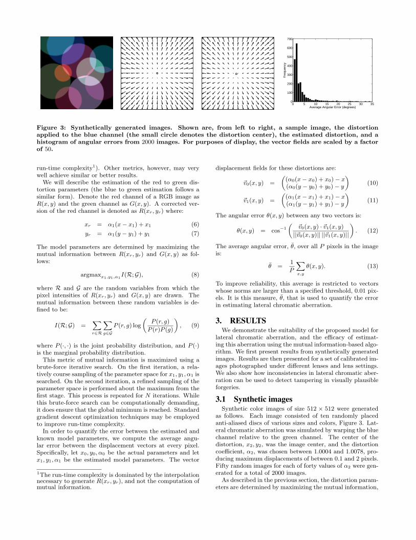
Figure 3: Synthetically generated images. Shown are, from left to right, a sample image, the distortionapplied to the blue channel (the small circle denotes the distortion center), the estimated distortion, and ahistogram of angular errors from 2000 images. For purposes of display, the vector fields are scaled by a factorof 50.
run-time complexity1). Other metrics, however, may verywell achieve similar or better results.
We will describe the estimation of the red to green dis-tortion parameters (the blue to green estimation follows asimilar form). Denote the red channel of a RGB image asR(x, y) and the green channel as G(x, y). A corrected ver-sion of the red channel is denoted as R(xr, yr) where:
xr = α1(x− x1) + x1 (6)
yr = α1(y − y1) + y1 (7)
The model parameters are determined by maximizing themutual information between R(xr, yr) and G(x, y) as fol-lows:
argmaxx1,y1,α1I(R;G), (8)
where R and G are the random variables from which thepixel intensities of R(xr, yr) and G(x, y) are drawn. Themutual information between these random variables is de-fined to be:
I(R;G) =Xr∈R
Xg∈G
P (r, g) log
„P (r, g)
P (r)P (g)
«, (9)
where P (·, ·) is the joint probability distribution, and P (·)is the marginal probability distribution.
This metric of mutual information is maximized using abrute-force iterative search. On the first iteration, a rela-tively course sampling of the parameter space for x1, y1, α1 issearched. On the second iteration, a refined sampling of theparameter space is performed about the maximum from thefirst stage. This process is repeated for N iterations. Whilethis brute-force search can be computationally demanding,it does ensure that the global minimum is reached. Standardgradient descent optimization techniques may be employedto improve run-time complexity.
In order to quantify the error between the estimated andknown model parameters, we compute the average angu-lar error between the displacement vectors at every pixel.Specifically, let x0, y0, α0 be the actual parameters and letx1, y1, α1 be the estimated model parameters. The vector
1The run-time complexity is dominated by the interpolationnecessary to generate R(xr, yr), and not the computation ofmutual information.
displacement fields for these distortions are:
~v0(x, y) =
„(α0(x− x0) + x0)− x(α0(y − y0) + y0)− y
«(10)
~v1(x, y) =
„(α1(x− x1) + x1)− x(α1(y − y1) + y1)− y
«(11)
The angular error θ(x, y) between any two vectors is:
θ(x, y) = cos−1
„~v0(x, y) · ~v1(x, y)
||~v0(x, y)|| ||~v1(x, y)||
«. (12)
The average angular error, θ, over all P pixels in the imageis:
θ =1
P
Xx,y
θ(x, y). (13)
To improve reliability, this average is restricted to vectorswhose norms are larger than a specified threshold, 0.01 pix-els. It is this measure, θ, that is used to quantify the errorin estimating lateral chromatic aberration.
3. RESULTSWe demonstrate the suitability of the proposed model for
lateral chromatic aberration, and the efficacy of estimat-ing this aberration using the mutual information-based algo-rithm. We first present results from synthetically generatedimages. Results are then presented for a set of calibrated im-ages photographed under different lenses and lens settings.We also show how inconsistencies in lateral chromatic aber-ration can be used to detect tampering in visually plausibleforgeries.
3.1 Synthetic imagesSynthetic color images of size 512 × 512 were generated
as follows. Each image consisted of ten randomly placedanti-aliased discs of various sizes and colors, Figure 3. Lat-eral chromatic aberration was simulated by warping the bluechannel relative to the green channel. The center of thedistortion, x2, y2, was the image center, and the distortioncoefficient, α2, was chosen between 1.0004 and 1.0078, pro-ducing maximum displacements of between 0.1 and 2 pixels.Fifty random images for each of forty values of α2 were gen-erated for a total of 2000 images.
As described in the previous section, the distortion param-eters are determined by maximizing the mutual information,
Equation (9), for the blue to green distortion. On the firstiteration of the brute-force search algorithm, values of x2, y2
spanning the entire image were considered, and values of α2
between 1.0002 to 1.02 were considered. Nine iterations ofthe search algorithm were performed, with the search spaceconsecutively refined on each iteration.
Shown in the second and third panels of Figure 3 are ex-amples of the applied and estimated distortion (the smallcircle denotes the distortion center). Shown in the fourthpanel of Figure 3 is the distribution of average angular er-rors from 2000 images. The average error is 3.4 degrees with93% of the errors less than 10 degrees. These results demon-strate the general efficacy of the mutual information-basedalgorithm for estimating lateral chromatic aberration.
3.2 Calibrated imagesIn order to test the efficacy of our approach on real im-
ages, we first estimated the lateral chromatic aberration fortwo lenses at various focal lengths and apertures. A 6.3mega-pixel Nikon D-100 digital camera was equipped witha Nikkor 18–35mm ED lens and a Nikkor 70–300mm EDlens2. For the 18–35 mm lens, focal lengths of 18, 24, 28,and 35 mm with 17 f -stops, ranging from f/29 to f/3.5,per focal length were considered. For the 70–300 mm lens,focal lengths of 70, 100, 135, 200, and 300 with 19 f -stops,ranging from f/45 to f/4, per focal length were considered.
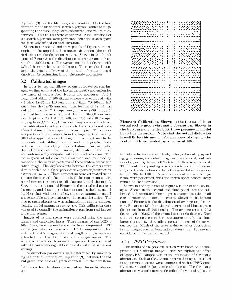
A calibration target was constructed of a peg board with1/4-inch diameter holes spaced one inch apart. The camerawas positioned at a distance from the target so that roughly500 holes appeared in each image. This target was back-illuminated with diffuse lighting, and photographed witheach lens and lens setting described above. For each colorchannel of each calibration image, the center of the holeswere automatically computed with sub-pixel resolution. Thered to green lateral chromatic aberration was estimated bycomparing the relative positions of these centers across theentire image. The displacements between the centers werethen modeled as a three parameter expansion/contractionpattern, x1, y1, α1. These parameters were estimated usinga brute force search that minimized the root mean squareerror between the measured displacements and the model.Shown in the top panel of Figure 4 is the actual red to greendistortion, and shown in the bottom panel is the best modelfit. Note that while not perfect, the three parameter modelis a reasonable approximation to the actual distortion. Theblue to green aberration was estimated in a similar manner,yielding model parameters x2, y2, α2. This calibration datawas used to quantify the estimation errors from real imagesof natural scenes.
Images of natural scenes were obtained using the samecamera and calibrated lenses. These images, of size 3020×2008 pixels, were captured and stored in uncompressed TIFFformat (see below for the effects of JPEG compression). Foreach of the 205 images, the focal length and f -stop wereextracted from the EXIF data in the image header. Theestimated aberration from each image was then comparedwith the corresponding calibration data with the same lenssettings.
The distortion parameters were determined by maximiz-ing the mutual information, Equation (9), between the redand green, and blue and green channels. On the first itera-
2ED lenses help to eliminate secondary chromatic aberra-tion.
Figure 4: Calibration. Shown in the top panel is anactual red to green chromatic aberration. Shown inthe bottom panel is the best three parameter modelfit to this distortion. Note that the actual distortionis well fit by this model. For purposes of display, thevector fields are scaled by a factor of 100.
tion of the brute-force search algorithm, values of x1, y1 andx2, y2 spanning the entire image were considered, and val-ues of α1 and α2 between 0.9985 to 1.0015 were considered.The bounds on α1 and α2 were chosen to include the entirerange of the distortion coefficient measured during calibra-tion, 0.9987 to 1.0009. Nine iterations of the search algo-rithm were performed, with the search space consecutivelyrefined on each iteration.
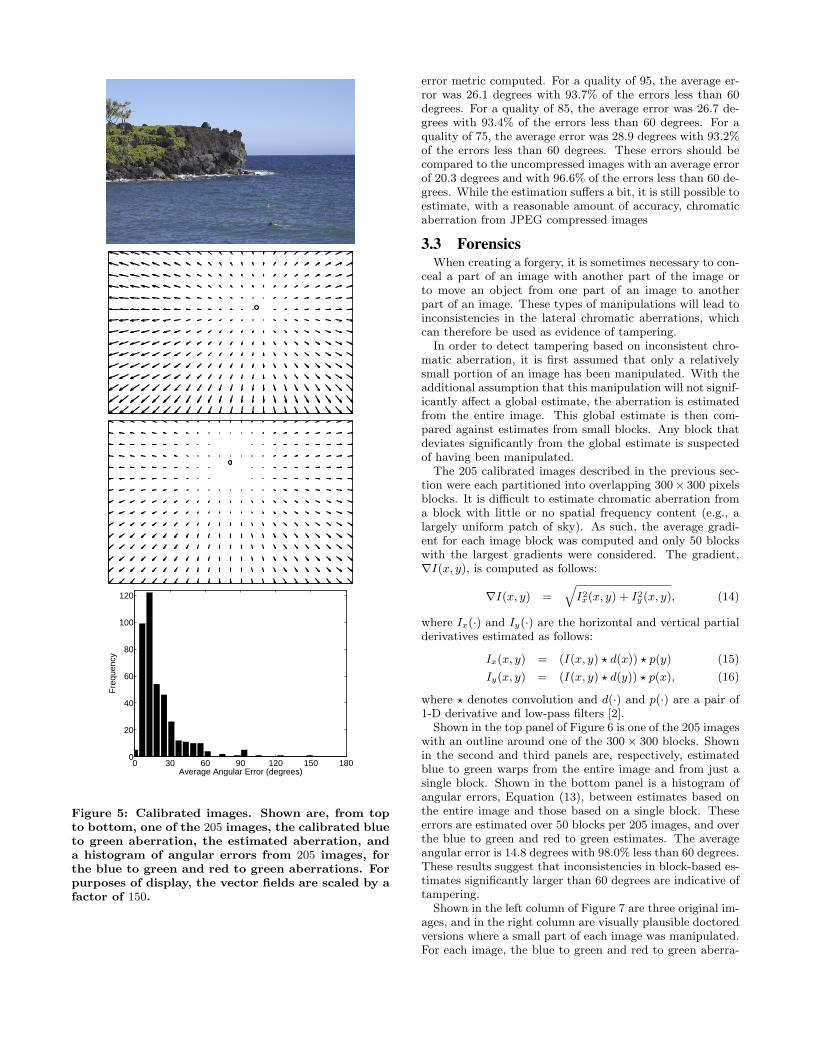
Shown in the top panel of Figure 5 is one of the 205 im-ages. Shown in the second and third panels are the cali-brated and estimated blue to green distortions (the smallcircle denotes the distortion center). Shown in the bottompanel of Figure 5 is the distribution of average angular er-rors, Equation (13), from the red to green and blue to greendistortions from all 205 images. The average error is 20.3degrees with 96.6% of the errors less than 60 degrees. Notethat the average errors here are approximately six timeslarger than the synthetically generated images of the previ-ous section. Much of the error is due to other aberrationsin the images, such as longitudinal aberration, that are notconsidered in our current model.
3.2.1 JPEG CompressionThe results of the previous section were based on uncom-
pressed TIFF format images. Here we explore the effectof lossy JPEG compression on the estimation of chromaticaberration. Each of the 205 uncompressed images describedin the previous section were compressed with a JPEG qual-ity of 95, 85, and 75 (on a scale of 1 to 100). The chromaticaberration was estimated as described above, and the same
0 30 60 90 120 150 1800
20
40
60
80
100
120
Average Angular Error (degrees)
Fre
quen
cy
Figure 5: Calibrated images. Shown are, from topto bottom, one of the 205 images, the calibrated blueto green aberration, the estimated aberration, anda histogram of angular errors from 205 images, forthe blue to green and red to green aberrations. Forpurposes of display, the vector fields are scaled by afactor of 150.
error metric computed. For a quality of 95, the average er-ror was 26.1 degrees with 93.7% of the errors less than 60degrees. For a quality of 85, the average error was 26.7 de-grees with 93.4% of the errors less than 60 degrees. For aquality of 75, the average error was 28.9 degrees with 93.2%of the errors less than 60 degrees. These errors should becompared to the uncompressed images with an average errorof 20.3 degrees and with 96.6% of the errors less than 60 de-grees. While the estimation suffers a bit, it is still possible toestimate, with a reasonable amount of accuracy, chromaticaberration from JPEG compressed images
3.3 ForensicsWhen creating a forgery, it is sometimes necessary to con-
ceal a part of an image with another part of the image orto move an object from one part of an image to anotherpart of an image. These types of manipulations will lead toinconsistencies in the lateral chromatic aberrations, whichcan therefore be used as evidence of tampering.
In order to detect tampering based on inconsistent chro-matic aberration, it is first assumed that only a relativelysmall portion of an image has been manipulated. With theadditional assumption that this manipulation will not signif-icantly affect a global estimate, the aberration is estimatedfrom the entire image. This global estimate is then com-pared against estimates from small blocks. Any block thatdeviates significantly from the global estimate is suspectedof having been manipulated.
The 205 calibrated images described in the previous sec-tion were each partitioned into overlapping 300× 300 pixelsblocks. It is difficult to estimate chromatic aberration froma block with little or no spatial frequency content (e.g., alargely uniform patch of sky). As such, the average gradi-ent for each image block was computed and only 50 blockswith the largest gradients were considered. The gradient,∇I(x, y), is computed as follows:
∇I(x, y) =q
I2x(x, y) + I2
y(x, y), (14)
where Ix(·) and Iy(·) are the horizontal and vertical partialderivatives estimated as follows:
Ix(x, y) = (I(x, y) ? d(x)) ? p(y) (15)
Iy(x, y) = (I(x, y) ? d(y)) ? p(x), (16)
where ? denotes convolution and d(·) and p(·) are a pair of1-D derivative and low-pass filters [2].
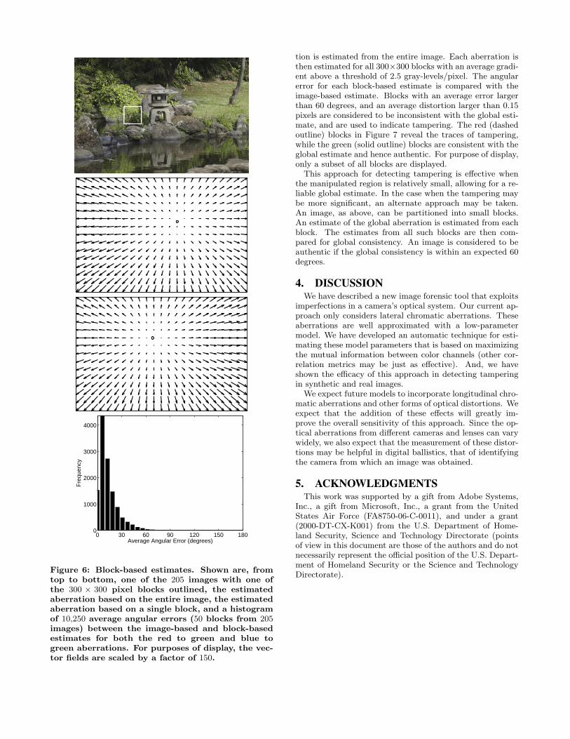
Shown in the top panel of Figure 6 is one of the 205 imageswith an outline around one of the 300× 300 blocks. Shownin the second and third panels are, respectively, estimatedblue to green warps from the entire image and from just asingle block. Shown in the bottom panel is a histogram ofangular errors, Equation (13), between estimates based onthe entire image and those based on a single block. Theseerrors are estimated over 50 blocks per 205 images, and overthe blue to green and red to green estimates. The averageangular error is 14.8 degrees with 98.0% less than 60 degrees.These results suggest that inconsistencies in block-based es-timates significantly larger than 60 degrees are indicative oftampering.
Shown in the left column of Figure 7 are three original im-ages, and in the right column are visually plausible doctoredversions where a small part of each image was manipulated.For each image, the blue to green and red to green aberra-
0 30 60 90 120 150 1800
1000
2000
3000
4000
Average Angular Error (degrees)
Fre
quen
cy
Figure 6: Block-based estimates. Shown are, fromtop to bottom, one of the 205 images with one ofthe 300 × 300 pixel blocks outlined, the estimatedaberration based on the entire image, the estimatedaberration based on a single block, and a histogramof 10,250 average angular errors (50 blocks from 205images) between the image-based and block-basedestimates for both the red to green and blue togreen aberrations. For purposes of display, the vec-tor fields are scaled by a factor of 150.
tion is estimated from the entire image. Each aberration isthen estimated for all 300×300 blocks with an average gradi-ent above a threshold of 2.5 gray-levels/pixel. The angularerror for each block-based estimate is compared with theimage-based estimate. Blocks with an average error largerthan 60 degrees, and an average distortion larger than 0.15pixels are considered to be inconsistent with the global esti-mate, and are used to indicate tampering. The red (dashedoutline) blocks in Figure 7 reveal the traces of tampering,while the green (solid outline) blocks are consistent with theglobal estimate and hence authentic. For purpose of display,only a subset of all blocks are displayed.
This approach for detecting tampering is effective whenthe manipulated region is relatively small, allowing for a re-liable global estimate. In the case when the tampering maybe more significant, an alternate approach may be taken.An image, as above, can be partitioned into small blocks.An estimate of the global aberration is estimated from eachblock. The estimates from all such blocks are then com-pared for global consistency. An image is considered to beauthentic if the global consistency is within an expected 60degrees.
4. DISCUSSIONWe have described a new image forensic tool that exploits
imperfections in a camera’s optical system. Our current ap-proach only considers lateral chromatic aberrations. Theseaberrations are well approximated with a low-parametermodel. We have developed an automatic technique for esti-mating these model parameters that is based on maximizingthe mutual information between color channels (other cor-relation metrics may be just as effective). And, we haveshown the efficacy of this approach in detecting tamperingin synthetic and real images.
We expect future models to incorporate longitudinal chro-matic aberrations and other forms of optical distortions. Weexpect that the addition of these effects will greatly im-prove the overall sensitivity of this approach. Since the op-tical aberrations from different cameras and lenses can varywidely, we also expect that the measurement of these distor-tions may be helpful in digital ballistics, that of identifyingthe camera from which an image was obtained.
5. ACKNOWLEDGMENTSThis work was supported by a gift from Adobe Systems,
Inc., a gift from Microsoft, Inc., a grant from the UnitedStates Air Force (FA8750-06-C-0011), and under a grant(2000-DT-CX-K001) from the U.S. Department of Home-land Security, Science and Technology Directorate (pointsof view in this document are those of the authors and do notnecessarily represent the official position of the U.S. Depart-ment of Homeland Security or the Science and TechnologyDirectorate).
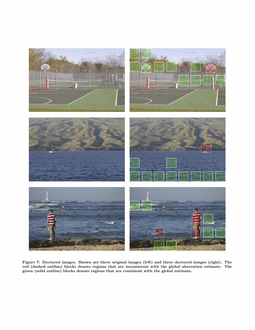
Figure 7: Doctored images. Shown are three original images (left) and three doctored images (right). Thered (dashed outline) blocks denote regions that are inconsistent with the global aberration estimate. Thegreen (solid outline) blocks denote regions that are consistent with the global estimate.
Appendix AHere we derive the 1-D and 2-D models of lateral chromaticaberration of Equations (2) and (3).
Consider in 1-D, Figure 1, where the incident light reachesthe lens at an angle θ, and is split into short wavelength(solid blue ray) and long wavelength (dashed red ray) lightwith an angle of refraction of θr and θb. These rays strikethe sensor at positions xr and xb. The relationship betweenthe angle of incidence and angles of refraction are given bySnell’s law, Equation (1), yielding:
sin(θ) = nr sin(θr) (17)
sin(θ) = nb sin(θb), (18)
which are combined to yield:
nr sin(θr) = nb sin(θb). (19)
Dividing both sides by cos(θb) gives:
nr sin(θr)/ cos(θb) = nb tan(θb)
= nbxb/f, (20)
where f is the lens-to-sensor distance. If we assume that thedifferences in angles of refraction are relatively small, thencos(θb) ≈ cos(θr). Equation (20) then takes the form:
nr sin(θr)/ cos(θr) ≈ nbxb/f
nr tan(θr) ≈ nbxb/f
nrxr/f ≈ nbxb/f
nrxr ≈ nbxb
xr ≈ αxb, (21)
where α = nb/nr.In 2-D, an incident ray reaches the lens at angles θ and
φ, relative to the x = 0 and y = 0 planes, respectively. Theapplication of Snell’s law yields:
nr sin(θr) = nb sin(θb) (22)
nr sin(φr) = nb sin(φb). (23)
Following the above 1-D derivation yields the following 2-Dmodel:
(xr, yr) ≈ α(xb, yb). (24)
6. REFERENCES[1] T. E. Boult and G. Wolberg. Correcting chromatic
aberrations using image warping. In Proceedings of theIEEE Conference on Computer Vision and PatternRecognition, pages 684–687, 1992.
[2] H. Farid and E. Simoncelli. Differentiation ofmulti-dimensional signals. IEEE Transactions onImage Processing, 13(4):496–508, 2004.
[3] J. Fridrich, D. Soukal, and J. Lukas. Detection ofcopy-move forgery in digital images. In Proceedings ofDFRWS, 2003.
[4] E. Hecht. Optics. Addison-Wesley PublishingCompany, Inc., 4th edition, 2002.
[5] M. K. Johnson and H. Farid. Exposing digitalforgeries by detecting inconsistencies in lighting. InACM Multimedia and Security Workshop, New York,NY, 2005.
[6] J. Lukas, J. Fridrich, and M. Goljan. Detecting digitalimage forgeries using sensor pattern noise. InProceedings of the SPIE, volume 6072, 2006.
[7] T. Ng and S. Chang. A model for image splicing. InIEEE International Conference on Image Processing,Singapore, 2004.
[8] A. C. Popescu and H. Farid. Exposing digital forgeriesby detecting duplicated image regions. TechnicalReport TR2004-515, Department of ComputerScience, Dartmouth College, 2004.
[9] A. C. Popescu and H. Farid. Exposing digital forgeriesby detecting traces of resampling. IEEE Transactionson Signal Processing, 53(2):758–767, 2005.
[10] A. C. Popescu and H. Farid. Exposing digital forgeriesin color filter array interpolated images. IEEETransactions on Signal Processing, 53(10):3948–3959,2005.
[11] P. Viola and W. M. Wells, III. Alignment bymaximization of mutual information. InternationalJournal of Computer Vision, 24(2):137–154, 1997.
[12] R. G. Willson and S. A. Shafer. What is the center ofthe image? Journal of the Optical Society of AmericaA, 11(11):2946–2955, November 1994.