exploring the functional composition of the human
TRANSCRIPT

Exploring the functional composition of the human microbiome using a hand‑curated microbial trait databaseJake L. Weissman1, Sonia Dogra1, Keyan Javadi1, Samantha Bolten1, Rachel Flint1, Cyrus Davati1, Jess Beattie1, Keshav Dixit1, Tejasvi Peesay1, Shehar Awan1, Peter Thielen2, Florian Breitwieser2, Philip L. F. Johnson1, David Karig3, William F. Fagan1 and Sharon Bewick4*
BackgroundMicrobial communities serve important functional roles in systems ranging from the human body [1], to rhizospheres [2], up to entire ecosystems [3]. Common goals of microbiome research are to determine factors shaping microbial community assembly,
Abstract
Background: Even when microbial communities vary wildly in their taxonomic com-position, their functional composition is often surprisingly stable. This suggests that a functional perspective could provide much deeper insight into the principles govern-ing microbiome assembly. Much work to date analyzing the functional composition of microbial communities, however, relies heavily on inference from genomic features. Unfortunately, output from these methods can be hard to interpret and often suffers from relatively high error rates.
Results: We built and analyzed a domain-specific microbial trait database from known microbe-trait pairs recorded in the literature to better understand the functional com-position of the human microbiome. Using a combination of phylogentically conscious machine learning tools and a network science approach, we were able to link particular traits to areas of the human body, discover traits that determine the range of body areas a microbe can inhabit, and uncover drivers of metabolic breadth.
Conclusions: Domain-specific trait databases are an effective compromise between noisy methods to infer complex traits from genomic data and exhaustive, expensive attempts at database curation from the literature that do not focus on any one subset of taxa. They provide an accurate account of microbial traits and, by limiting the num-ber of taxa considered, are feasible to build within a reasonable time-frame. We present a database specific for the human microbiome, in the hopes that this will prove useful for research into the functional composition of human-associated microbial communities.
Keywords: Trait database, Functional community, Random forest, Phylogenetic correction
Open Access
© The Author(s), 2021. Open Access This article is licensed under a Creative Commons Attribution 4.0 International License, which permits use, sharing, adaptation, distribution and reproduction in any medium or format, as long as you give appropriate credit to the original author(s) and the source, provide a link to the Creative Commons licence, and indicate if changes were made. The images or other third party material in this article are included in the article’s Creative Commons licence, unless indicated otherwise in a credit line to the mate-rial. If material is not included in the article’s Creative Commons licence and your intended use is not permitted by statutory regulation or exceeds the permitted use, you will need to obtain permission directly from the copyright holder. To view a copy of this licence, visit http:// creat iveco mmons. org/ licen ses/ by/4. 0/. The Creative Commons Public Domain Dedication waiver (http:// creat iveco mmons. org/ publi cdoma in/ zero/1. 0/) applies to the data made available in this article, unless otherwise stated in a credit line to the data.
RESEARCH ARTICLE
Weissman et al. BMC Bioinformatics (2021) 22:306 https://doi.org/10.1186/s12859‑021‑04216‑2
*Correspondence: [email protected] 4 Biological Sciences Department, Clemson University, Clemson, SC, USAFull list of author information is available at the end of the article

Page 2 of 21Weissman et al. BMC Bioinformatics (2021) 22:306
and also how changes in the makeup of a community lead to changes in its overall behavior. Often, it is safe to assume that organisms with similar traits may fill similar roles, even if they are only distantly related. Thus, if we want to measure the relation-ship between composition and behavior, it makes sense to prioritize functional over taxonomic composition [4]. In fact, a number of studies have shown that, across nearly identical environments, taxonomic composition can be highly variable, while functional composition is largely constant. This suggests that most habitats are dominated by a sta-ble, core functional community [5, 6].
Typically, functional analysis of microbial communities relies on genetic inference of microbial traits, specifically metabolic traits (e.g. [7]). Often, these inference meth-ods suffer from high error rates [8, 9]. Additionally, for even moderately complex traits such as aerobicity, it is extremely difficult to make inferences from genomic data [10]. Obviously, hand-curated databases such as ours have the disadvantage of being labor-intensive to construct [11]. Others have attempted to get around this problem by using automated text-mining approaches that assign confidence levels to particular traits in specific microbes [12]. At least for type strains, however, functional information avail-able in the literature is much better defined than automated text-mining databases imply [13]. Consequently, it is possible to assign traits to microbes with a quite high degree of confidence if one is willing to put in the time to curate the trait database. We take this laborious but precise approach and curate a domain-specific database for human associ-ated microbes (Additional file 1). By limiting the scope of our database, we reduce the number of microbial species that we need to consider, allowing us to compile a reason-ably large number of traits for an entire system of imminent importance.
We demonstrate the utility of our trait database with a number of analyses drawing on tools from machine learning and network science. As a first step we characterize the functional traits associated with different sites across the human body (e.g., stool, poste-rior fornix, buccal mucosa) and identify suites of traits that frequently co-occur across communities in those sites. We then build predictive models to associate specific traits with the number of body areas (e.g., gut, vagina, mouth) across which a species is found. Finally, we explore how metabolic diversity varies across sites, and predict the metabolic breadth of a species from its other traits. In all cases we adopt a phylogenetically con-scious framework in which we correct model performance measures to account for non-independence due to shared evolutionary history [14].
ResultsRevealing body‑site versus trait associations
We used three complementary approaches to reveal associations of specific traits with specific body sites: (1) pairwise comparisons of mean trait values between body sites, (2) predictive modeling of sample source sites with random forests, and (3) network-based clustering of traits.
Pairwise comparisons between body sites
As seen in Figs. 1 and 2, many traits differed between body sites, even given our restriction that differences must appear across multiple phyla (see Additional file 2: S2 Fig and S3 Fig for traits with differences shown individually across all phyla, and

Page 3 of 21Weissman et al. BMC Bioinformatics (2021) 22:306
Additional file 2: S4 Fig and S5 Fig for results on all phyla together). This is not sur-prising, given that different body sites provide very different environments (nutrients, temperature, oxygen, etc.) and are home to communities with very different taxo-nomic compositions. In keeping with pairwise results, samples clustered functionally according to body site (see Additional file 2: S1 Fig). This is similar to the results seen for taxonomic composition [15].
Some of the trends that emerged from pairwise comparisons were as expected based on knowledge of site characteristics. For example, the prevalence of anaer-obes was higher in the gut (stool), a low oxygen environment, relative to other body sites. Other trends, however, reveal novel biology. Ammonia production, for instance, is under-represented in stool, while production of hydrogen sulfide gas is
a b
Fig. 1 Pairwise differences in trait values between body sites (difference in means weighted by taxon abundance). Interactions that were not significant in at least two phyla are left blank. Traits separated into categories for readability: a qualitative with categorical values (split into dummy variables for multi-level traits) and b quantitative with continous values. For carbon substrate use traits see Fig. 2
Fig. 2 Pairwise differences in carbon substrate use frequency between body sites (difference in means weighted by taxon abundance). Interactions that were not significant in at least two phyla are left blank. Shown here are binary traits indicating the ability to grow on specific carbon sources. For other traits see Fig. 1

Page 4 of 21Weissman et al. BMC Bioinformatics (2021) 22:306
under-represented across the mouth (buccal mucosa, supragingival plaque and the tongue dorsum). Although there were no clear trends in carbon substrate metabolism across compound classes (e.g., alcohols, sugars), what did emerge from our carbon substrate analysis was the relative uniqueness of the different body sites in terms of resource use (see Fig. 2). This led us to build predictive models to identify those traits that most uniquely define the different locations on the human body.
Predictive modeling of sample source
We were able to build separate models to predict, with reasonable accuracy, if a sample came from the stool, posterior fornix, or anterior nares (Cohen’s κ from phylogeneti-cally-blocked cross validation: 0.436, 0.416, and 0.379 respectively; Table 1). By contrast, similar models for the mouth performed poorly ( κ = 0.170 ), and we were entirely una-ble to predict whether a sample came from the skin (Table 1). Difficulties with oral and skin microbiomes are likely due to the fact that trait values vary more across phyla in the mouth than at other body sites (Additional file 2: S6 Fig), and because we had very few skin samples with which to train our model (17). In fact, by restricting our analysis to only those traits that vary relatively little between phyla, we were able to increase our overall predictive ability in samples from the mouth (0.373; Additional file 2: S1 Table). To some extent, the high degree of variation in traits across phyla from the mouth prob-ably stems from the variability in site types across the oral microbiome (tongue, plaque, etc.). However, even when we considered habitats separately, we were unable to predict whether a sample was from a specific site (tongue, plaque, or buccal mucosa), suggesting that, at least for the functions considered in our database, the functional compositions of the different oral microbial communities are similar.
In all models, predictive ability varied across phyla. For example, while we were able to predict whether a sample came from stool based on resident Firmicutes, we were not able to do so based on resident Proteobacteria (Table 1). This may not come as a surprise, because while Proteobacteria do appear in the human gut microbiome, their abundance is typically low and their presence unreliable across individuals [16, 17]. This makes them sub-optimal predictors of sample source site.
Table 1 Cohen’s κ for predicting sample source site
Briefly, the trait values associated with a set of three phyla in a sample were used to train a model to predict whether a sample was from a given site on the basis of a fourth “test” phylum. Values above zero indicate predictive ability in excess of a null model accounting for the number of samples from each site
Test Mean
Actinobacteria Bacteroidetes Firmicutes Proteobacteria
Stool 0.350 0.468 0.948 − 0.021 0.436
Posterior Fornix 0.340 0.351 0.560 0.413 0.416
Anterior Nares 0.430 0.579 0.268 0.240 0.379
Retroauricular Crease 0.165 0 0.033 0.038 0.059
Tongue Dorsum 0 0 0.019 0 0.005
Supragingival Plaque 0 0 0.157 0 0.039
Buccal Mucosa 0 0 0 0 0
Mouth (All) 0 0 0.677 0.004 0.170

Page 5 of 21Weissman et al. BMC Bioinformatics (2021) 22:306
A number of variables were important for predicting the source site of a body sample, regardless of the set of phyla used (Additional file 2: S7 Fig, S8 Fig, S9 Fig, and S10 Fig). In Fig. 3, S11 Fig, S12 Fig, and S13 Fig we show plots of a selection of the strongest pre-dictors across phyla for our high-performing models (stool, fornix, nares, and mouth, respectively). For example, in keeping with our pairwise analysis, the strongest predictor of a sample being from stool was a highly anaerobic resident community. Not unexpect-edly, optimal temperature was also highest in stool and lowest in the mouth. Meanwhile, optimal pH was lowest in stool and highest in the mouth. Further, in keeping with the hypothesis that the gut is a complex environment, genome size was generally larger in stool and, accordingly, cell volume was also larger in this habitat. Importantly, our ran-dom forest identified traits associated with particular sites whose effects may be non-linear or context dependent (e.g., pH in the stool, formate in the anterior nares; Fig. 3, Additional file 2: S11 Fig, S12 Fig, S13 Fig). Mirroring the result in S6 Fig, the top predic-tors from the mouth models varied more across taxa than the top predictors for other sites (Additional file 2: S14 Fig).
��������
��
��������������������
��
������������
��
������
��
��
��
����
����
��
��������
��
��
��
��
��
��
��
��
��
��
��
��
��
��������
��
����
����
��
��
��
��
��
��
��
��
����
��
��
��
��
��
��
��
��
��
��
����
��
����
��
��
��
��
����
��
��
����
��
��
����
��
����
����
��
��
��
��
��
��
��
��
����
��
����
��
��
��
��
��
��
��
��
��������������������������������
��
��
��
����
��
������������������
������
��
��
������
��
��
��
��
��
��
��
��
��
��
��
����
��
��
����
��
��
��
��
��
��
������
��
��
��
��
����
��
����
��
��
��
��
��
��
��
��
��
��
��
��
��
��
��
����
��
��
��
��������
��
��
��
��
��
��
��
��
��
����
��
����
��
��
��
����
��
��
����
��
����
��
����
��
��
��
0.00
0.25
0.50
0.75
1.00
Anterior_nare
s
Buccal_mucosa
Posterior_forn
ix
Retroauricular_crea
seStool
Supra
gingival_plaque
Tongue_dorsum
Ana
erob
e
1
��
��
��
��
��
��
��
��
��
��
��
��
��
��
����
��
����
����
��
����
��
��
����
��
��
��
��
��
��
����
��
��
����
����
��
��
����
��
��
��
��
��
��
����������������������������������������������
��
��
����
��
��
��
��
��
��
����������
��������������������
��
��
��
����
��
����������
��
����
��
��
��
��
��
������
��
����
��
��
��
������
��
����
��
��������������
��
��
��
��
��
��������
��
��
��
��
��
��
����
������
��
��������
��
��
��
��
��
��
��
��
��
��
��
��
��������
����
����
��������
��
������
��
����
25
30
35
40
45
Anterior_nare
s
Buccal_mucosa
Posterior_forn
ix
Retroauricular_crea
seStool
Supra
gingival_plaque
Tongue_dorsum
Opt
imal
Tem
p.
2
��
������������
��
������
������������
��
��������
��
��
������������������������
��
��
��������
��
��
��������������������
��
��
��
��
��
��
����
��
��
��
��
��
��
��
��
����
����
����
��
��
��������
��
0.0
2.5
5.0
7.5
Anterior_nare
s
Buccal_mucosa
Posterior_forn
ix
Retroauricular_crea
seStool
Supra
gingival_plaque
Tongue_dorsum
Leng
thMajorAxis
3
����
��
��
��
��
��
��
��
����
��
��
��
��
��
����
��������
��
��
��
����
��
����
��������������������������������������������������������������������������������������������������������������������������������������������������������������
2e+06
3e+06
4e+06
5e+06
6e+06
7e+06
Anterior_nare
s
Buccal_mucosa
Posterior_forn
ix
Retroauricular_crea
seStool
Supra
gingival_plaque
Tongue_dorsum
Gen
ome
Leng
th
4
����������������
����
����
��
��
��
��
��
����
��
��
����
��
���� ����5
6
7
8
Anterior_nare
s
Buccal_mucosa
Posterior_forn
ix
Retroauricular_crea
seStool
Supra
gingival_plaque
Tongue_dorsum
Opt
imal
pH
5������
������������������������
������������
��
����������
��
����������
������������������
������������������������
����
������
����
30
40
50
60
Anterior_nare
s
Buccal_mucosa
Posterior_forn
ix
Retroauricular_crea
seStool
Supra
gingival_plaque
Tongue_dorsum
GC
Con
tent
6
Fig. 3 Top predictors for stool with rank shown in upper left corner. Top predictors across phyla of sample source site, for which importance scores are above the average variable importance across all predictors for all four training sets (7). Shown are mean trait values across all samples in the dataset, split up by body site. See 11, 12, and 13 for top predictors of posterior fornix, anterior nares, and mouth respectively

Page 6 of 21Weissman et al. BMC Bioinformatics (2021) 22:306
Networks linking body sites to suites of traits
We inferred a network of trait associations based on the abundance of traits across sam-ples (Additional file 2: S15 Fig). We then performed neighborhood detection to find clusters of traits that tend to covary across samples (Table 2). These clusters represent suites of traits that can be associated with a particular environment (Fig. 4, Additional file 2: S16 Fig). The combined use of butyrate and caprate, for example, are strongly neg-atively associated with the tongue and, to a lesser extent, the posterior fornix. Instead, the tongue is strongly associated with the combined use of adonitol and alanine. Mean-while, the posterior fornix is associated with a complex set of traits including use of ara-binose, propionate, rhamnose, succinate, and xylose, as well as production of indole and hydrogen sulfide. Interestingly, this suite of traits is positively associated with many body sites, including the nares, the tongue and stool.
Generalism versus trait associations
Some human-associated microbes are found in a single body area, while others are broadly distributed across the entire human body. One hypothesis for why this might be is that there are certain traits that allow generalist species to live everywhere. To explore this possibility, we attempted to predict whether species were habitat specialists or gen-eralists using trait data. For simplicity, we defined specialists as species that appeared in samples from only a single body area and generalists as species that appeared in samples from at least two body areas (see Methods). Specifically, we built random forest models and used blocked cross validation to obtain a phylogenetically corrected estimate of our prediction accuracy (Fig. 5). When using phylogenetically-blocked cross validation, folds correspond to clusters of related taxa (e.g., phyla, classes) rather than being chosen at random. Some phyla were more predictable than others. We predicted reasonably well whether members of Actinobacteria were generalists using the other phyla as a train-ing set. For other phyla (Bacteroidetes, Firmicutes, and Proteobacteria), we were less
MucosaFornix NaresSkinStool Plaque Tongue
34 5 121416 1711 15 2 7 10 18
Fig. 4 Bipartite site-cluster network, where clusters are groups of traits that frequently co-occur. Clusters are shown at the top as blue, numbered nodes. Each cluster corresponds to a group of co-occuring traits as listed in Table 2. Body sites are shown at the bottom as labeled, yellow nodes. Positive interactions (cluster common in body site) are represented by solid green lines and negative interactions (cluster uncommon in body site) are represented by dotted red lines. The strength of an interaction is represented by the with of an edge. See 16 for the same figure with positive and negative interactions separated out for ease of viewing

Page 7 of 21Weissman et al. BMC Bioinformatics (2021) 22:306
successful. However, even for most of these phyla (Firmicutes and Proteobacteria), we were able to predict across Classes (see values for Cohen’s κ ). Ironically, due to the rela-tively small number of taxa in our dataset from Actinobacteria our models performed worse when predicting within this phylum as opposed to across phyla (which requires further subdivision via cross-validation and lowers training set size).
The most important predictors varied between phyla, with little overlap (Additional file 2: S17 Fig). The exception was cell aggregation which took categorical values of chain, clump, and single, and which showed up as one of the top 5 most important pre-dictors for three out of four phyla. Overall, however, it appears that the traits important for predicting generalism vary across phyla as a rule.
We followed up our predictive approach with individual parametric tests for phy-logenetically significant trait versus generalism associations in each phylum using phylogenetic logistic regression (see Methods). Given the steep dropoff in importance
Table 2 Inferred trait clusters with positive associations between body sites
Bold and starred ( ⋆ ) site names signify that a given cluster‑site interaction is the strongest positive interaction observed for that site
Cluster Traits Positive associations
2 Use of: alaninamide, histidine, leucine, pyruvic acid methyl ester
3 OptimalpH, Facultative, Cocci, Use of:fructose, galactose, glucose, Buccal mucosa, Tongue
lactose, mannose, methyl beta D glucoside, N acetylglucosa-mine, sucrose
Anterior nares, Supragingival plaque
4 LengthMajorAxis, Enzyme Assays: esculin aesculin hydrolysis, Posterior fornix
Use of: cellobiose, glycogen, maltose, raffinose, salicin, starch, yeast extract
5 Max. Temp., Optimal NaCl, Min. NaCl, Max. NaCl, Genome Length, Anaerobe, Single, Clump, Rod,
Stool,
Enzyme Assays: urease, acid phosphatase, alkaline phosphatase, alpha galactosidase,
Posterior fornix,
beta galactosidase, acetoin, phosphatase, DNA degradation, Gas Production: indole, hydrogen sulfide,
Retroauricular crease,
Use of: arabinose, propionate, rhamnose, succinate, Tween 80, xylose
Anterior nares, Tongue
7 Use of: phenylacetate, putrescine, quinic acid Supragingival plaque10 Use of: arginine, glycine, phenylalanine, serine, threonine Tongue
11 Min. pH, Max. pH Posterior fornix
12 Enzyme Assays: tellurite reductase, Use of: citrate
14 Optimal Temp., Enzyme Assays: gelatinase, trypsin, Anterior nares,
Use of: acetate, galacturonate, glycerol, lactate, Retroauricular crease,
mannitol, melibiose, ornithine, ribose, sorbitol, trehalose Supragingival plaque, Tongue
15 Use of: butanol, caprate
16 GC Content, Min. Temp., Motile, Aerobe, Chain, Gas Production: ammonia, isovaleric acid,
Retroauricular crease,
Enzyme Assays: catalase, oxidase, arylsulfatase, phosphohydro-lase,
Supragingival plaque,
Use of: aspartate, dextrin, formate, glutamate, malate, proline, pyruvate, suberate, urea, sugars
Tongue
17 Use of: adonitol, alanine Tongue18 Use of: valerate, 2 aminethanol, 2 ketogluconate, 2 3 butanediol, Tongue
3 hydroxybenzoate, 3 hydroxybutyrate, 4 hydroxybenzoate, 5 ketogluconate

Page 8 of 21Weissman et al. BMC Bioinformatics (2021) 22:306
after the top few predictors in Additional file 2: S17 Fig, we tested the top five most important traits for predicting whether members of each phylum were specialists, and corrected for multiple testing (Benjamini-Hochberg control of FDR, α = 0.05 , p-cutoff = 0.021). For the Actinobacteria, the trait found to be a significant predic-tor of generalism was being an facultative anaerobe ( p = 0.0005 , Coefficient = 1.3), whereas being an obligate anaerobe ( p = 0.0002 , Coefficient = − 1.5) was associ-ated with body site restriction. This makes sense, since facultative anaerobes are more flexible overall, and since a large number of human body sites are exposed to oxygen. For Bacteroidetes, the significant traits associated with generalism were the abilities to use yeast extract ( p = 0.0023 , Coefficient = − 0.72) and aspartate ( p = 0.0069 , Coefficient = −0.55 ), as well as β-galactosidase ( p = 0.0101 , Coefficient = 0.73), and alkaline phosphatase ( p = 0.0014 , Coefficient = 0.83) activity. Like Act-inobacteria, generalist Firmcutes were also more likely to be facultative anaerobes ( p = 0.0102, Coefficient = 0.72 ), while specialists were more likely to be obligate anaerobes ( p = 0.0094, Coefficient = −0.75 ) Other traits predictive of generalism for Firmicutes were having a small genome length ( p = 0.0003, Coefficient = −1.4 ), and a low GC content ( p = 0.0191, Coefficient = −0.78 ). For Proteobacteria the only significant trait associated with generalism was minimum growth temperature ( p = 0.0197, Coefficient = 0.84).
Metabolism
Metabolic breadth - the number of substrates used by a particular microbiome - is a measure of the diversity of functions and the flexibility of the microbial community. As such, it reflects microbiome complexity, which may, itself, be a reflection of the
�
All
Actinob
acteria
Bac
teroidetes
Firm
icutes
Proteob
acteria
−0.5
0.0
0.5
1.0
Coh
en's
κ
����
��
��
��
��
�
�
All
Actinob
acteria
Bac
teroidetes
Firm
icutes
Proteob
acteria
0.3
0.4
0.5
0.6
0.7
0.8
0.9
1.0
AUCPR
����
��
����
��
�
All
Actinob
acteria
Bac
teroidetes
Firm
icutes
Proteob
acteria
0.0
0.2
0.4
0.6
0.8
1.0
P(S
pecialist)
��
����
��
��
��
Fig. 5 Performance of random forest models predicting generalism (binary classification, present at more than one area or not). “All” means a blocked cross-validation with each phylum as a fold (Actinobacteria: red squares, Bacteroidetes: green triangles, Firmicutes: blue diamonds, Proteobacteria: purple circles). Within each phylum we performed blocked cross-validation using classes as folds, except in the case of Bacteroidetes where all species in the dataset were in the same class and order, so that families were used as the folds. Shown are two measures of performance ( κ and area under the precision-recall curve), as well as the prevalence of specialist species in a fold ( P(Specialist) for “probability is a specialist”)

Page 9 of 21Weissman et al. BMC Bioinformatics (2021) 22:306
complexity of environmental conditions and/or resource inputs into the system. Below, we consider metabolic breadth, first across body sites, and then across microbial taxa.
Metabolic breadth across sites
Different body sites differ in the overall number of carbon substrates used by their resident microbes, with a high coverage of carbon sources in stool and the majority of oral sites and a much lower coverage of carbon sources in skin, nares and vaginal sites (Fig. 6). There are three proximate reasons why metabolic breadth could be increased in
��
����
����
����
��
��
��
��
��
������
��
1
2
3Re
troauricular_crease
Anterior_nares
Posterior_fornix
Mid_vagina
Vaginal_intro
itus
Keratinize
d_gingiva
Buccal_m
ucosa
Stool
Throat
Supragingival_plaque
Tongue_dorsum
Saliva
Subgingival_plaque
Palatine_Tonsils
Entr
opy
over
Car
bon
Met
abol
ism
s in
a S
ampl
e
��
��
��
��
��
���� ��
��
��
20
40
60
80
Retro
auricular_crease
Anterior_nares
Posterior_fornix
Mid_vagina
Vaginal_intro
itus
Keratinize
d_gingiva
Buccal_m
ucosa
Stool
Throat
Supragingival_plaque
Tongue_dorsum
Saliva
Subgingival_plaque
Palatine_TonsilsRic
hnes
s of
Car
bon
Met
abol
ism
s in
a S
ampl
e
����
��
��
����
����
����
��
���������� ��
0.2
0.4
0.6
0.8
1.0
Retro
auricular_crease
Anterior_nares
Posterior_fornix
Mid_vagina
Vaginal_intro
itus
Keratinize
d_gingiva
Buccal_m
ucosa
Stool
Throat
Supragingival_plaque
Tongue_dorsum
Saliva
Subgingival_plaque
Palatine_TonsilsPe
ilou'
s Ev
enes
s of
Car
bon
Met
abol
ism
s
��
��
��
��
����
��
��
����
��
��
0
1
2
3
Retro
auricular_crease
Anterior_nares
Posterior_fornix
Mid_vagina
Vaginal_intro
itus
Keratinize
d_gingiva
Buccal_m
ucosa
Stool
Throat
Supragingival_plaque
Tongue_dorsum
Saliva
Subgingival_plaque
Palatine_Tonsils
Entr
opy
over
Spe
cies
in a
Sam
ple
��
��
��
��
����
������
����
��
��
��
0
50
100
Retro
auricular_crease
Anterior_nares
Posterior_fornix
Mid_vagina
Vaginal_intro
itus
Keratinize
d_gingiva
Buccal_m
ucosa
Stool
Throat
Supragingival_plaque
Tongue_dorsum
Saliva
Subgingival_plaque
Palatine_Tonsils
Ric
hnes
s of
Spe
cies
in a
Sam
ple
��
��
��
��
��
��
��
����������
��
��
0.0
0.2
0.4
0.6
0.8
Retro
auricular_crease
Anterior_nares
Posterior_fornix
Mid_vagina
Vaginal_intro
itus
Keratinize
d_gingiva
Buccal_m
ucosa
Stool
Throat
Supragingival_plaque
Tongue_dorsum
Saliva
Subgingival_plaque
Palatine_Tonsils
Peilo
u's
Even
ess
of S
peci
es
��
�
��
��
��
�
����
�
��
��
��
��
��
��
��
������
�
��
��
���
��
��
��
��
��
��
�
��
��
��
��
�
��
��
��
�
��
��
��
�
�
�
��
��
� �
��
����
�
�
�
��
�
�
���
��
��
��
��
�
��
��
��
�
�
��
�
�
��
��
�
��
��
��
�
��
�
��
��
�
��
��
�
�
��
�
��
���
��
��
�
���
��
��
�
��
�
��
��
���
�
��
��
��
����
��
��
���
��
��
����
��
��
�
�
���
�
�
��
�
��
�
��
�
�
��
�
��
��
��
����
�
�
��
��
��
��
��
�� �
��
����
�
��
��
��
��
��
���
�
��
��
��
��
��
����
�
��
��
��
��
��
�
��
��
�
��
�
��
��
��
������
��
�
��
�
�
�
��
��
�
��
��
��
��
��
��
�
��
��
��
��
�
��
��
��
��
�
��
��
��
���
�
��
��
�
�
���
��
�
��
��
��
��
�
��
��
��
��
��
��
��
��
��
��
��
�
��
�
����
��
��
�
��
��
��
��
��
�
��
��
�
��
��
��
��
�
��
��
��
�
�
��
��
�
��
�
��
��
��
��
�
�
��
���
�
��
��
���
��
��
��
��
��
����
�
���
��
��
��
�
��
��
�� �
��
��
��
��
�
��
��
�
�
���
��
�
�
��
�
�
��
��
�
��
�
��
��
��
����
��
��
��
��
�
��
��
��
�
��
��
�
�
��
��
��
��
�
��
��
��
�
��
��
�
��
��
��
��
��
�
��
�
��
�
��
���
�
�
�� �
��
��
��
��
��
��
��
���
�
��
��
��
�
��
���
��
��
��
�
��
����
��
��
�
��
��
�
��
�
��
��
�� ��
��
��
��
��
��
��
��
��
��
���
�
��
��
� �
��
��
�� ��
��
�
��
�
��
��
��
��
��
��
��
��
��
�
��
��
��
��
��
�
��
��
����
�
�
��
�
��
��
�
��
��
�
���
�
�
��
�
��
��
�
��
�
���
������
������������������������������������
������������������������
�������������������������������������������������������������������������������������������������������������������������������������������������������������
��������������������������
�����������������������������
������������������������������������������������������������������������������������������������������������������������������������������������������ ����
�
�
�
�
���
�
��������
�
�
�
����
�
�
�������
��������
��������������
�
����������
���
���������
����������������������
����� �����
������������
� �������������������
���
��������������������������������
���������������������������������
��������
�������
�
����������������������������������������������������������������������������������������������������������������������������������������������
��
�����������
�
�
�
�
���
��
�������
�
����
�
����������
������������������������������������������������������������������������
�����������������������������������������������������
���������������������������������������������������������������������������������������������������������������������������
������������������������������������������������������������������������������������������
�������
����
�
�������������������������������������
�
�
�����������������������������
��������
�������������������
�������������������
r2 = 0.726r2 = 0.726r2 = 0.726r2 = 0.726r2 = 0.726r2 = 0.726r2 = 0.726r2 = 0.726r2 = 0.726r2 = 0.726r2 = 0.726r2 = 0.726r2 = 0.726r2 = 0.726r2 = 0.726r2 = 0.726r2 = 0.726r2 = 0.726r2 = 0.726r2 = 0.726r2 = 0.726r2 = 0.726r2 = 0.726r2 = 0.726r2 = 0.726r2 = 0.726r2 = 0.726r2 = 0.726r2 = 0.726r2 = 0.726r2 = 0.726r2 = 0.726r2 = 0.726r2 = 0.726r2 = 0.726r2 = 0.726r2 = 0.726r2 = 0.726r2 = 0.726r2 = 0.726r2 = 0.726r2 = 0.726r2 = 0.726r2 = 0.726r2 = 0.726r2 = 0.726r2 = 0.726r2 = 0.726r2 = 0.726r2 = 0.726r2 = 0.726r2 = 0.726r2 = 0.726r2 = 0.726r2 = 0.726r2 = 0.726r2 = 0.726r2 = 0.726r2 = 0.726r2 = 0.726r2 = 0.726r2 = 0.726r2 = 0.726r2 = 0.726r2 = 0.726r2 = 0.726r2 = 0.726r2 = 0.726r2 = 0.726r2 = 0.726r2 = 0.726r2 = 0.726r2 = 0.726r2 = 0.726r2 = 0.726r2 = 0.726r2 = 0.726r2 = 0.726r2 = 0.726r2 = 0.726r2 = 0.726r2 = 0.726r2 = 0.726r2 = 0.726r2 = 0.726r2 = 0.726r2 = 0.726r2 = 0.726r2 = 0.726r2 = 0.726r2 = 0.726r2 = 0.726r2 = 0.726r2 = 0.726r2 = 0.726r2 = 0.726r2 = 0.726r2 = 0.726r2 = 0.726r2 = 0.726r2 = 0.726r2 = 0.726r2 = 0.726r2 = 0.726r2 = 0.726r2 = 0.726r2 = 0.726r2 = 0.726r2 = 0.726r2 = 0.726r2 = 0.726r2 = 0.726r2 = 0.726r2 = 0.726r2 = 0.726r2 = 0.726r2 = 0.726r2 = 0.726r2 = 0.726r2 = 0.726r2 = 0.726r2 = 0.726r2 = 0.726r2 = 0.726r2 = 0.726r2 = 0.726r2 = 0.726r2 = 0.726r2 = 0.726r2 = 0.726r2 = 0.726r2 = 0.726r2 = 0.726r2 = 0.726r2 = 0.726r2 = 0.726r2 = 0.726r2 = 0.726r2 = 0.726r2 = 0.726r2 = 0.726r2 = 0.726r2 = 0.726r2 = 0.726r2 = 0.726r2 = 0.726r2 = 0.726r2 = 0.726r2 = 0.726r2 = 0.726r2 = 0.726r2 = 0.726r2 = 0.726r2 = 0.726r2 = 0.726r2 = 0.726r2 = 0.726r2 = 0.726r2 = 0.726r2 = 0.726r2 = 0.726r2 = 0.726r2 = 0.726r2 = 0.726r2 = 0.726r2 = 0.726r2 = 0.726r2 = 0.726r2 = 0.726r2 = 0.726r2 = 0.726r2 = 0.726r2 = 0.726r2 = 0.726r2 = 0.726r2 = 0.726r2 = 0.726r2 = 0.726r2 = 0.726r2 = 0.726r2 = 0.726r2 = 0.726r2 = 0.726r2 = 0.726r2 = 0.726r2 = 0.726r2 = 0.726r2 = 0.726r2 = 0.726r2 = 0.726r2 = 0.726r2 = 0.726r2 = 0.726r2 = 0.726r2 = 0.726r2 = 0.726r2 = 0.726r2 = 0.726r2 = 0.726r2 = 0.726r2 = 0.726r2 = 0.726r2 = 0.726r2 = 0.726r2 = 0.726r2 = 0.726r2 = 0.726r2 = 0.726r2 = 0.726r2 = 0.726r2 = 0.726r2 = 0.726r2 = 0.726r2 = 0.726r2 = 0.726r2 = 0.726r2 = 0.726r2 = 0.726r2 = 0.726r2 = 0.726r2 = 0.726r2 = 0.726r2 = 0.726r2 = 0.726r2 = 0.726r2 = 0.726r2 = 0.726r2 = 0.726r2 = 0.726r2 = 0.726r2 = 0.726r2 = 0.726r2 = 0.726r2 = 0.726r2 = 0.726r2 = 0.726r2 = 0.726r2 = 0.726r2 = 0.726r2 = 0.726r2 = 0.726r2 = 0.726r2 = 0.726r2 = 0.726r2 = 0.726r2 = 0.726r2 = 0.726r2 = 0.726r2 = 0.726r2 = 0.726r2 = 0.726r2 = 0.726r2 = 0.726r2 = 0.726r2 = 0.726r2 = 0.726r2 = 0.726r2 = 0.726r2 = 0.726r2 = 0.726r2 = 0.726r2 = 0.726r2 = 0.726r2 = 0.726r2 = 0.726r2 = 0.726r2 = 0.726r2 = 0.726r2 = 0.726r2 = 0.726r2 = 0.726r2 = 0.726r2 = 0.726r2 = 0.726r2 = 0.726r2 = 0.726r2 = 0.726r2 = 0.726r2 = 0.726r2 = 0.726r2 = 0.726r2 = 0.726r2 = 0.726r2 = 0.726r2 = 0.726r2 = 0.726r2 = 0.726r2 = 0.726r2 = 0.726r2 = 0.726r2 = 0.726r2 = 0.726r2 = 0.726r2 = 0.726r2 = 0.726r2 = 0.726r2 = 0.726r2 = 0.726r2 = 0.726r2 = 0.726r2 = 0.726r2 = 0.726r2 = 0.726r2 = 0.726r2 = 0.726r2 = 0.726r2 = 0.726r2 = 0.726r2 = 0.726r2 = 0.726r2 = 0.726r2 = 0.726r2 = 0.726r2 = 0.726r2 = 0.726r2 = 0.726r2 = 0.726r2 = 0.726r2 = 0.726r2 = 0.726r2 = 0.726r2 = 0.726r2 = 0.726r2 = 0.726r2 = 0.726r2 = 0.726r2 = 0.726r2 = 0.726r2 = 0.726r2 = 0.726r2 = 0.726r2 = 0.726r2 = 0.726r2 = 0.726r2 = 0.726r2 = 0.726r2 = 0.726r2 = 0.726r2 = 0.726r2 = 0.726r2 = 0.726r2 = 0.726r2 = 0.726r2 = 0.726r2 = 0.726r2 = 0.726r2 = 0.726r2 = 0.726r2 = 0.726r2 = 0.726r2 = 0.726r2 = 0.726r2 = 0.726r2 = 0.726r2 = 0.726r2 = 0.726r2 = 0.726r2 = 0.726r2 = 0.726r2 = 0.726r2 = 0.726r2 = 0.726r2 = 0.726r2 = 0.726r2 = 0.726r2 = 0.726r2 = 0.726r2 = 0.726r2 = 0.726r2 = 0.726r2 = 0.726r2 = 0.726r2 = 0.726r2 = 0.726r2 = 0.726r2 = 0.726r2 = 0.726r2 = 0.726r2 = 0.726r2 = 0.726r2 = 0.726r2 = 0.726r2 = 0.726r2 = 0.726r2 = 0.726r2 = 0.726r2 = 0.726r2 = 0.726r2 = 0.726r2 = 0.726r2 = 0.726r2 = 0.726r2 = 0.726r2 = 0.726r2 = 0.726r2 = 0.726r2 = 0.726r2 = 0.726r2 = 0.726r2 = 0.726r2 = 0.726r2 = 0.726r2 = 0.726r2 = 0.726r2 = 0.726r2 = 0.726r2 = 0.726r2 = 0.726r2 = 0.726r2 = 0.726r2 = 0.726r2 = 0.726r2 = 0.726r2 = 0.726r2 = 0.726r2 = 0.726r2 = 0.726r2 = 0.726r2 = 0.726r2 = 0.726r2 = 0.726r2 = 0.726r2 = 0.726r2 = 0.726r2 = 0.726r2 = 0.726r2 = 0.726r2 = 0.726r2 = 0.726r2 = 0.726r2 = 0.726r2 = 0.726r2 = 0.726r2 = 0.726r2 = 0.726r2 = 0.726r2 = 0.726r2 = 0.726r2 = 0.726r2 = 0.726r2 = 0.726r2 = 0.726r2 = 0.726r2 = 0.726r2 = 0.726r2 = 0.726r2 = 0.726r2 = 0.726r2 = 0.726r2 = 0.726r2 = 0.726r2 = 0.726r2 = 0.726r2 = 0.726r2 = 0.726r2 = 0.726r2 = 0.726r2 = 0.726r2 = 0.726r2 = 0.726r2 = 0.726r2 = 0.726r2 = 0.726r2 = 0.726r2 = 0.726r2 = 0.726r2 = 0.726r2 = 0.726r2 = 0.726r2 = 0.726r2 = 0.726r2 = 0.726r2 = 0.726r2 = 0.726r2 = 0.726r2 = 0.726r2 = 0.726r2 = 0.726r2 = 0.726r2 = 0.726r2 = 0.726r2 = 0.726r2 = 0.726r2 = 0.726r2 = 0.726r2 = 0.726r2 = 0.726r2 = 0.726p = 7.48e−139p = 7.48e−139p = 7.48e−139p = 7.48e−139p = 7.48e−139p = 7.48e−139p = 7.48e−139p = 7.48e−139p = 7.48e−139p = 7.48e−139p = 7.48e−139p = 7.48e−139p = 7.48e−139p = 7.48e−139p = 7.48e−139p = 7.48e−139p = 7.48e−139p = 7.48e−139p = 7.48e−139p = 7.48e−139p = 7.48e−139p = 7.48e−139p = 7.48e−139p = 7.48e−139p = 7.48e−139p = 7.48e−139p = 7.48e−139p = 7.48e−139p = 7.48e−139p = 7.48e−139p = 7.48e−139p = 7.48e−139p = 7.48e−139p = 7.48e−139p = 7.48e−139p = 7.48e−139p = 7.48e−139p = 7.48e−139p = 7.48e−139p = 7.48e−139p = 7.48e−139p = 7.48e−139p = 7.48e−139p = 7.48e−139p = 7.48e−139p = 7.48e−139p = 7.48e−139p = 7.48e−139p = 7.48e−139p = 7.48e−139p = 7.48e−139p = 7.48e−139p = 7.48e−139p = 7.48e−139p = 7.48e−139p = 7.48e−139p = 7.48e−139p = 7.48e−139p = 7.48e−139p = 7.48e−139p = 7.48e−139p = 7.48e−139p = 7.48e−139p = 7.48e−139p = 7.48e−139p = 7.48e−139p = 7.48e−139p = 7.48e−139p = 7.48e−139p = 7.48e−139p = 7.48e−139p = 7.48e−139p = 7.48e−139p = 7.48e−139p = 7.48e−139p = 7.48e−139p = 7.48e−139p = 7.48e−139p = 7.48e−139p = 7.48e−139p = 7.48e−139p = 7.48e−139p = 7.48e−139p = 7.48e−139p = 7.48e−139p = 7.48e−139p = 7.48e−139p = 7.48e−139p = 7.48e−139p = 7.48e−139p = 7.48e−139p = 7.48e−139p = 7.48e−139p = 7.48e−139p = 7.48e−139p = 7.48e−139p = 7.48e−139p = 7.48e−139p = 7.48e−139p = 7.48e−139p = 7.48e−139p = 7.48e−139p = 7.48e−139p = 7.48e−139p = 7.48e−139p = 7.48e−139p = 7.48e−139p = 7.48e−139p = 7.48e−139p = 7.48e−139p = 7.48e−139p = 7.48e−139p = 7.48e−139p = 7.48e−139p = 7.48e−139p = 7.48e−139p = 7.48e−139p = 7.48e−139p = 7.48e−139p = 7.48e−139p = 7.48e−139p = 7.48e−139p = 7.48e−139p = 7.48e−139p = 7.48e−139p = 7.48e−139p = 7.48e−139p = 7.48e−139p = 7.48e−139p = 7.48e−139p = 7.48e−139p = 7.48e−139p = 7.48e−139p = 7.48e−139p = 7.48e−139p = 7.48e−139p = 7.48e−139p = 7.48e−139p = 7.48e−139p = 7.48e−139p = 7.48e−139p = 7.48e−139p = 7.48e−139p = 7.48e−139p = 7.48e−139p = 7.48e−139p = 7.48e−139p = 7.48e−139p = 7.48e−139p = 7.48e−139p = 7.48e−139p = 7.48e−139p = 7.48e−139p = 7.48e−139p = 7.48e−139p = 7.48e−139p = 7.48e−139p = 7.48e−139p = 7.48e−139p = 7.48e−139p = 7.48e−139p = 7.48e−139p = 7.48e−139p = 7.48e−139p = 7.48e−139p = 7.48e−139p = 7.48e−139p = 7.48e−139p = 7.48e−139p = 7.48e−139p = 7.48e−139p = 7.48e−139p = 7.48e−139p = 7.48e−139p = 7.48e−139p = 7.48e−139p = 7.48e−139p = 7.48e−139p = 7.48e−139p = 7.48e−139p = 7.48e−139p = 7.48e−139p = 7.48e−139p = 7.48e−139p = 7.48e−139p = 7.48e−139p = 7.48e−139p = 7.48e−139p = 7.48e−139p = 7.48e−139p = 7.48e−139p = 7.48e−139p = 7.48e−139p = 7.48e−139p = 7.48e−139p = 7.48e−139p = 7.48e−139p = 7.48e−139p = 7.48e−139p = 7.48e−139p = 7.48e−139p = 7.48e−139p = 7.48e−139p = 7.48e−139p = 7.48e−139p = 7.48e−139p = 7.48e−139p = 7.48e−139p = 7.48e−139p = 7.48e−139p = 7.48e−139p = 7.48e−139p = 7.48e−139p = 7.48e−139p = 7.48e−139p = 7.48e−139p = 7.48e−139p = 7.48e−139p = 7.48e−139p = 7.48e−139p = 7.48e−139p = 7.48e−139p = 7.48e−139p = 7.48e−139p = 7.48e−139p = 7.48e−139p = 7.48e−139p = 7.48e−139p = 7.48e−139p = 7.48e−139p = 7.48e−139p = 7.48e−139p = 7.48e−139p = 7.48e−139p = 7.48e−139p = 7.48e−139p = 7.48e−139p = 7.48e−139p = 7.48e−139p = 7.48e−139p = 7.48e−139p = 7.48e−139p = 7.48e−139p = 7.48e−139p = 7.48e−139p = 7.48e−139p = 7.48e−139p = 7.48e−139p = 7.48e−139p = 7.48e−139p = 7.48e−139p = 7.48e−139p = 7.48e−139p = 7.48e−139p = 7.48e−139p = 7.48e−139p = 7.48e−139p = 7.48e−139p = 7.48e−139p = 7.48e−139p = 7.48e−139p = 7.48e−139p = 7.48e−139p = 7.48e−139p = 7.48e−139p = 7.48e−139p = 7.48e−139p = 7.48e−139p = 7.48e−139p = 7.48e−139p = 7.48e−139p = 7.48e−139p = 7.48e−139p = 7.48e−139p = 7.48e−139p = 7.48e−139p = 7.48e−139p = 7.48e−139p = 7.48e−139p = 7.48e−139p = 7.48e−139p = 7.48e−139p = 7.48e−139p = 7.48e−139p = 7.48e−139p = 7.48e−139p = 7.48e−139p = 7.48e−139p = 7.48e−139p = 7.48e−139p = 7.48e−139p = 7.48e−139p = 7.48e−139p = 7.48e−139p = 7.48e−139p = 7.48e−139p = 7.48e−139p = 7.48e−139p = 7.48e−139p = 7.48e−139p = 7.48e−139p = 7.48e−139p = 7.48e−139p = 7.48e−139p = 7.48e−139p = 7.48e−139p = 7.48e−139p = 7.48e−139p = 7.48e−139p = 7.48e−139p = 7.48e−139p = 7.48e−139p = 7.48e−139p = 7.48e−139p = 7.48e−139p = 7.48e−139p = 7.48e−139p = 7.48e−139p = 7.48e−139p = 7.48e−139p = 7.48e−139p = 7.48e−139p = 7.48e−139p = 7.48e−139p = 7.48e−139p = 7.48e−139p = 7.48e−139p = 7.48e−139p = 7.48e−139p = 7.48e−139p = 7.48e−139p = 7.48e−139p = 7.48e−139p = 7.48e−139p = 7.48e−139p = 7.48e−139p = 7.48e−139p = 7.48e−139p = 7.48e−139p = 7.48e−139p = 7.48e−139p = 7.48e−139p = 7.48e−139p = 7.48e−139p = 7.48e−139p = 7.48e−139p = 7.48e−139p = 7.48e−139p = 7.48e−139p = 7.48e−139p = 7.48e−139p = 7.48e−139p = 7.48e−139p = 7.48e−139p = 7.48e−139p = 7.48e−139p = 7.48e−139p = 7.48e−139p = 7.48e−139p = 7.48e−139p = 7.48e−139p = 7.48e−139p = 7.48e−139p = 7.48e−139p = 7.48e−139p = 7.48e−139p = 7.48e−139p = 7.48e−139p = 7.48e−139p = 7.48e−139p = 7.48e−139p = 7.48e−139p = 7.48e−139p = 7.48e−139p = 7.48e−139p = 7.48e−139p = 7.48e−139p = 7.48e−139p = 7.48e−139p = 7.48e−139p = 7.48e−139p = 7.48e−139p = 7.48e−139p = 7.48e−139p = 7.48e−139p = 7.48e−139p = 7.48e−139p = 7.48e−139p = 7.48e−139p = 7.48e−139p = 7.48e−139p = 7.48e−139p = 7.48e−139p = 7.48e−139p = 7.48e−139p = 7.48e−139p = 7.48e−139p = 7.48e−139p = 7.48e−139p = 7.48e−139p = 7.48e−139p = 7.48e−139p = 7.48e−139p = 7.48e−139p = 7.48e−139p = 7.48e−139p = 7.48e−139p = 7.48e−139p = 7.48e−139p = 7.48e−139p = 7.48e−139p = 7.48e−139p = 7.48e−139p = 7.48e−139p = 7.48e−139p = 7.48e−139p = 7.48e−139p = 7.48e−139p = 7.48e−139p = 7.48e−139p = 7.48e−139p = 7.48e−139p = 7.48e−139p = 7.48e−139p = 7.48e−139p = 7.48e−139p = 7.48e−139p = 7.48e−139p = 7.48e−139p = 7.48e−139p = 7.48e−139p = 7.48e−139p = 7.48e−139p = 7.48e−139p = 7.48e−139p = 7.48e−139p = 7.48e−139p = 7.48e−139p = 7.48e−139p = 7.48e−139p = 7.48e−139p = 7.48e−139p = 7.48e−139p = 7.48e−139p = 7.48e−139p = 7.48e−139p = 7.48e−139p = 7.48e−139p = 7.48e−139p = 7.48e−139p = 7.48e−139p = 7.48e−139p = 7.48e−139p = 7.48e−139p = 7.48e−139p = 7.48e−139p = 7.48e−139p = 7.48e−139p = 7.48e−139p = 7.48e−139p = 7.48e−139p = 7.48e−139p = 7.48e−139p = 7.48e−139p = 7.48e−139p = 7.48e−139p = 7.48e−139p = 7.48e−139p = 7.48e−139p = 7.48e−139p = 7.48e−139p = 7.48e−139p = 7.48e−139p = 7.48e−139p = 7.48e−139p = 7.48e−139p = 7.48e−139p = 7.48e−139p = 7.48e−139p = 7.48e−139p = 7.48e−139p = 7.48e−139p = 7.48e−139p = 7.48e−139p = 7.48e−139p = 7.48e−139p = 7.48e−139p = 7.48e−1391
2
3
0 1 2 3Species Entropy
Car
bon
Entr
opy
��
�
��
��
��
�
��
����
�
��
��
�
�
��
��
��
��
��
��
��
�
��
��
��
��
�
��
�
��
��
��
�
�
��
���
�
�
�
�����
����
�� �
����
��
��
��
�
����
��
�����
�
��
��
��
���
�
��
��
�
��
��
��
�
��
��
��
�
��
��
��
�
�
��
�
�
��
��
��
������
��
��
�
��
�
��
��
���
��
��
��
�
� ��
��
�
�
�
�
��
�
��
��
��
�
��
��
����
��
�
�
��
��
��
��
����
���
�
��
��
� ��
��
��
�
�
�
��
�
��
��
���
�
��
��
��
��
����
��
��
��
�
��
��
��
�
�
����
��
� ��
��
��
����
�
��
�
��
��
��
�
��
��
�
���
��
�
�
��
��
�
��
��� �
��
�� �
��
��
��
��
��
�
�
��
��
���
��
��� �� �
��
�
��
��
�
��
�
��
��
��
�
��
�
��
�
��
�
��
�
�
��
��
�
�
��
��
��
����
��
��
��
��
�
��
��
�
�
�� ��
�
��
��
��
���
��
��
��
��
�
��
��
�
��
�
�
��
��
��
��
����
���
��
�
��
��
��
�
�
��
��
�
��
��
��
��
��
�
�
��
��
��
��
��
���
��
���
�
����
��
��
��
���
��
�
��
��
�
�
�
��
�
��
��
��
��
��
����
��
��
�
��
��
��
��
��
�
�
���
�
��
�
��
���
���
��
��
�
�
�
�
��
���
��
���
��
�����
��
��
��
��
��
���
��
��
��
��
��
��
�
��
��
��
�
�
���
��
��
��
�
��
��
�
��
��
�
�
��
��
��
�
�
��
��
��
���
��
��
�
��
��
��
��
�
��
��
��
��
�
��
��
�
�
��
��
��
�
��
��
�
��
��� ��
��
�
��
��
�����
����
��
����
��
��
��
��
�
��
��
��
��
��
��
��
��
��
�
��
���
��
�
��
��
��
�
��
��
���
��
��
��
����
��
��
�
�
������
���
����
�
�����
�����
���������������
�����������������
����������������������������
�� �������������
�������
��������������������������������������������
����������������
��
��������
����
�
�
����
������
�
�
���
��������������������
�����
���
���������������������������
������������
�
�������
���
�����������
��������
������
���
������
�������
������������������
��������
����������������
������
�������
����������������������������������
������������
���
�
��������������
�����������������������������������������������
��������������������������������������� ������
�����������������������������������������������
r2 = 0.795r2 = 0.795r2 = 0.795r2 = 0.795r2 = 0.795r2 = 0.795r2 = 0.795r2 = 0.795r2 = 0.795r2 = 0.795r2 = 0.795r2 = 0.795r2 = 0.795r2 = 0.795r2 = 0.795r2 = 0.795r2 = 0.795r2 = 0.795r2 = 0.795r2 = 0.795r2 = 0.795r2 = 0.795r2 = 0.795r2 = 0.795r2 = 0.795r2 = 0.795r2 = 0.795r2 = 0.795r2 = 0.795r2 = 0.795r2 = 0.795r2 = 0.795r2 = 0.795r2 = 0.795r2 = 0.795r2 = 0.795r2 = 0.795r2 = 0.795r2 = 0.795r2 = 0.795r2 = 0.795r2 = 0.795r2 = 0.795r2 = 0.795r2 = 0.795r2 = 0.795r2 = 0.795r2 = 0.795r2 = 0.795r2 = 0.795r2 = 0.795r2 = 0.795r2 = 0.795r2 = 0.795r2 = 0.795r2 = 0.795r2 = 0.795r2 = 0.795r2 = 0.795r2 = 0.795r2 = 0.795r2 = 0.795r2 = 0.795r2 = 0.795r2 = 0.795r2 = 0.795r2 = 0.795r2 = 0.795r2 = 0.795r2 = 0.795r2 = 0.795r2 = 0.795r2 = 0.795r2 = 0.795r2 = 0.795r2 = 0.795r2 = 0.795r2 = 0.795r2 = 0.795r2 = 0.795r2 = 0.795r2 = 0.795r2 = 0.795r2 = 0.795r2 = 0.795r2 = 0.795r2 = 0.795r2 = 0.795r2 = 0.795r2 = 0.795r2 = 0.795r2 = 0.795r2 = 0.795r2 = 0.795r2 = 0.795r2 = 0.795r2 = 0.795r2 = 0.795r2 = 0.795r2 = 0.795r2 = 0.795r2 = 0.795r2 = 0.795r2 = 0.795r2 = 0.795r2 = 0.795r2 = 0.795r2 = 0.795r2 = 0.795r2 = 0.795r2 = 0.795r2 = 0.795r2 = 0.795r2 = 0.795r2 = 0.795r2 = 0.795r2 = 0.795r2 = 0.795r2 = 0.795r2 = 0.795r2 = 0.795r2 = 0.795r2 = 0.795r2 = 0.795r2 = 0.795r2 = 0.795r2 = 0.795r2 = 0.795r2 = 0.795r2 = 0.795r2 = 0.795r2 = 0.795r2 = 0.795r2 = 0.795r2 = 0.795r2 = 0.795r2 = 0.795r2 = 0.795r2 = 0.795r2 = 0.795r2 = 0.795r2 = 0.795r2 = 0.795r2 = 0.795r2 = 0.795r2 = 0.795r2 = 0.795r2 = 0.795r2 = 0.795r2 = 0.795r2 = 0.795r2 = 0.795r2 = 0.795r2 = 0.795r2 = 0.795r2 = 0.795r2 = 0.795r2 = 0.795r2 = 0.795r2 = 0.795r2 = 0.795r2 = 0.795r2 = 0.795r2 = 0.795r2 = 0.795r2 = 0.795r2 = 0.795r2 = 0.795r2 = 0.795r2 = 0.795r2 = 0.795r2 = 0.795r2 = 0.795r2 = 0.795r2 = 0.795r2 = 0.795r2 = 0.795r2 = 0.795r2 = 0.795r2 = 0.795r2 = 0.795r2 = 0.795r2 = 0.795r2 = 0.795r2 = 0.795r2 = 0.795r2 = 0.795r2 = 0.795r2 = 0.795r2 = 0.795r2 = 0.795r2 = 0.795r2 = 0.795r2 = 0.795r2 = 0.795r2 = 0.795r2 = 0.795r2 = 0.795r2 = 0.795r2 = 0.795r2 = 0.795r2 = 0.795r2 = 0.795r2 = 0.795r2 = 0.795r2 = 0.795r2 = 0.795r2 = 0.795r2 = 0.795r2 = 0.795r2 = 0.795r2 = 0.795r2 = 0.795r2 = 0.795r2 = 0.795r2 = 0.795r2 = 0.795r2 = 0.795r2 = 0.795r2 = 0.795r2 = 0.795r2 = 0.795r2 = 0.795r2 = 0.795r2 = 0.795r2 = 0.795r2 = 0.795r2 = 0.795r2 = 0.795r2 = 0.795r2 = 0.795r2 = 0.795r2 = 0.795r2 = 0.795r2 = 0.795r2 = 0.795r2 = 0.795r2 = 0.795r2 = 0.795r2 = 0.795r2 = 0.795r2 = 0.795r2 = 0.795r2 = 0.795r2 = 0.795r2 = 0.795r2 = 0.795r2 = 0.795r2 = 0.795r2 = 0.795r2 = 0.795r2 = 0.795r2 = 0.795r2 = 0.795r2 = 0.795r2 = 0.795r2 = 0.795r2 = 0.795r2 = 0.795r2 = 0.795r2 = 0.795r2 = 0.795r2 = 0.795r2 = 0.795r2 = 0.795r2 = 0.795r2 = 0.795r2 = 0.795r2 = 0.795r2 = 0.795r2 = 0.795r2 = 0.795r2 = 0.795r2 = 0.795r2 = 0.795r2 = 0.795r2 = 0.795r2 = 0.795r2 = 0.795r2 = 0.795r2 = 0.795r2 = 0.795r2 = 0.795r2 = 0.795r2 = 0.795r2 = 0.795r2 = 0.795r2 = 0.795r2 = 0.795r2 = 0.795r2 = 0.795r2 = 0.795r2 = 0.795r2 = 0.795r2 = 0.795r2 = 0.795r2 = 0.795r2 = 0.795r2 = 0.795r2 = 0.795r2 = 0.795r2 = 0.795r2 = 0.795r2 = 0.795r2 = 0.795r2 = 0.795r2 = 0.795r2 = 0.795r2 = 0.795r2 = 0.795r2 = 0.795r2 = 0.795r2 = 0.795r2 = 0.795r2 = 0.795r2 = 0.795r2 = 0.795r2 = 0.795r2 = 0.795r2 = 0.795r2 = 0.795r2 = 0.795r2 = 0.795r2 = 0.795r2 = 0.795r2 = 0.795r2 = 0.795r2 = 0.795r2 = 0.795r2 = 0.795r2 = 0.795r2 = 0.795r2 = 0.795r2 = 0.795r2 = 0.795r2 = 0.795r2 = 0.795r2 = 0.795r2 = 0.795r2 = 0.795r2 = 0.795r2 = 0.795r2 = 0.795r2 = 0.795r2 = 0.795r2 = 0.795r2 = 0.795r2 = 0.795r2 = 0.795r2 = 0.795r2 = 0.795r2 = 0.795r2 = 0.795r2 = 0.795r2 = 0.795r2 = 0.795r2 = 0.795r2 = 0.795r2 = 0.795r2 = 0.795r2 = 0.795r2 = 0.795r2 = 0.795r2 = 0.795r2 = 0.795r2 = 0.795r2 = 0.795r2 = 0.795r2 = 0.795r2 = 0.795r2 = 0.795r2 = 0.795r2 = 0.795r2 = 0.795r2 = 0.795r2 = 0.795r2 = 0.795r2 = 0.795r2 = 0.795r2 = 0.795r2 = 0.795r2 = 0.795r2 = 0.795r2 = 0.795r2 = 0.795r2 = 0.795r2 = 0.795r2 = 0.795r2 = 0.795r2 = 0.795r2 = 0.795r2 = 0.795r2 = 0.795r2 = 0.795r2 = 0.795r2 = 0.795r2 = 0.795r2 = 0.795r2 = 0.795r2 = 0.795r2 = 0.795r2 = 0.795r2 = 0.795r2 = 0.795r2 = 0.795r2 = 0.795r2 = 0.795r2 = 0.795r2 = 0.795r2 = 0.795r2 = 0.795r2 = 0.795r2 = 0.795r2 = 0.795r2 = 0.795r2 = 0.795r2 = 0.795r2 = 0.795r2 = 0.795r2 = 0.795r2 = 0.795r2 = 0.795r2 = 0.795r2 = 0.795r2 = 0.795r2 = 0.795r2 = 0.795r2 = 0.795r2 = 0.795r2 = 0.795r2 = 0.795r2 = 0.795r2 = 0.795r2 = 0.795r2 = 0.795r2 = 0.795r2 = 0.795r2 = 0.795r2 = 0.795r2 = 0.795r2 = 0.795r2 = 0.795r2 = 0.795r2 = 0.795r2 = 0.795r2 = 0.795r2 = 0.795r2 = 0.795r2 = 0.795r2 = 0.795r2 = 0.795r2 = 0.795r2 = 0.795r2 = 0.795r2 = 0.795r2 = 0.795r2 = 0.795r2 = 0.795r2 = 0.795r2 = 0.795r2 = 0.795r2 = 0.795r2 = 0.795r2 = 0.795r2 = 0.795r2 = 0.795r2 = 0.795r2 = 0.795r2 = 0.795r2 = 0.795r2 = 0.795r2 = 0.795r2 = 0.795r2 = 0.795r2 = 0.795r2 = 0.795r2 = 0.795r2 = 0.795r2 = 0.795r2 = 0.795r2 = 0.795r2 = 0.795r2 = 0.795r2 = 0.795r2 = 0.795r2 = 0.795r2 = 0.795r2 = 0.795p = 2.29e−169p = 2.29e−169p = 2.29e−169p = 2.29e−169p = 2.29e−169p = 2.29e−169p = 2.29e−169p = 2.29e−169p = 2.29e−169p = 2.29e−169p = 2.29e−169p = 2.29e−169p = 2.29e−169p = 2.29e−169p = 2.29e−169p = 2.29e−169p = 2.29e−169p = 2.29e−169p = 2.29e−169p = 2.29e−169p = 2.29e−169p = 2.29e−169p = 2.29e−169p = 2.29e−169p = 2.29e−169p = 2.29e−169p = 2.29e−169p = 2.29e−169p = 2.29e−169p = 2.29e−169p = 2.29e−169p = 2.29e−169p = 2.29e−169p = 2.29e−169p = 2.29e−169p = 2.29e−169p = 2.29e−169p = 2.29e−169p = 2.29e−169p = 2.29e−169p = 2.29e−169p = 2.29e−169p = 2.29e−169p = 2.29e−169p = 2.29e−169p = 2.29e−169p = 2.29e−169p = 2.29e−169p = 2.29e−169p = 2.29e−169p = 2.29e−169p = 2.29e−169p = 2.29e−169p = 2.29e−169p = 2.29e−169p = 2.29e−169p = 2.29e−169p = 2.29e−169p = 2.29e−169p = 2.29e−169p = 2.29e−169p = 2.29e−169p = 2.29e−169p = 2.29e−169p = 2.29e−169p = 2.29e−169p = 2.29e−169p = 2.29e−169p = 2.29e−169p = 2.29e−169p = 2.29e−169p = 2.29e−169p = 2.29e−169p = 2.29e−169p = 2.29e−169p = 2.29e−169p = 2.29e−169p = 2.29e−169p = 2.29e−169p = 2.29e−169p = 2.29e−169p = 2.29e−169p = 2.29e−169p = 2.29e−169p = 2.29e−169p = 2.29e−169p = 2.29e−169p = 2.29e−169p = 2.29e−169p = 2.29e−169p = 2.29e−169p = 2.29e−169p = 2.29e−169p = 2.29e−169p = 2.29e−169p = 2.29e−169p = 2.29e−169p = 2.29e−169p = 2.29e−169p = 2.29e−169p = 2.29e−169p = 2.29e−169p = 2.29e−169p = 2.29e−169p = 2.29e−169p = 2.29e−169p = 2.29e−169p = 2.29e−169p = 2.29e−169p = 2.29e−169p = 2.29e−169p = 2.29e−169p = 2.29e−169p = 2.29e−169p = 2.29e−169p = 2.29e−169p = 2.29e−169p = 2.29e−169p = 2.29e−169p = 2.29e−169p = 2.29e−169p = 2.29e−169p = 2.29e−169p = 2.29e−169p = 2.29e−169p = 2.29e−169p = 2.29e−169p = 2.29e−169p = 2.29e−169p = 2.29e−169p = 2.29e−169p = 2.29e−169p = 2.29e−169p = 2.29e−169p = 2.29e−169p = 2.29e−169p = 2.29e−169p = 2.29e−169p = 2.29e−169p = 2.29e−169p = 2.29e−169p = 2.29e−169p = 2.29e−169p = 2.29e−169p = 2.29e−169p = 2.29e−169p = 2.29e−169p = 2.29e−169p = 2.29e−169p = 2.29e−169p = 2.29e−169p = 2.29e−169p = 2.29e−169p = 2.29e−169p = 2.29e−169p = 2.29e−169p = 2.29e−169p = 2.29e−169p = 2.29e−169p = 2.29e−169p = 2.29e−169p = 2.29e−169p = 2.29e−169p = 2.29e−169p = 2.29e−169p = 2.29e−169p = 2.29e−169p = 2.29e−169p = 2.29e−169p = 2.29e−169p = 2.29e−169p = 2.29e−169p = 2.29e−169p = 2.29e−169p = 2.29e−169p = 2.29e−169p = 2.29e−169p = 2.29e−169p = 2.29e−169p = 2.29e−169p = 2.29e−169p = 2.29e−169p = 2.29e−169p = 2.29e−169p = 2.29e−169p = 2.29e−169p = 2.29e−169p = 2.29e−169p = 2.29e−169p = 2.29e−169p = 2.29e−169p = 2.29e−169p = 2.29e−169p = 2.29e−169p = 2.29e−169p = 2.29e−169p = 2.29e−169p = 2.29e−169p = 2.29e−169p = 2.29e−169p = 2.29e−169p = 2.29e−169p = 2.29e−169p = 2.29e−169p = 2.29e−169p = 2.29e−169p = 2.29e−169p = 2.29e−169p = 2.29e−169p = 2.29e−169p = 2.29e−169p = 2.29e−169p = 2.29e−169p = 2.29e−169p = 2.29e−169p = 2.29e−169p = 2.29e−169p = 2.29e−169p = 2.29e−169p = 2.29e−169p = 2.29e−169p = 2.29e−169p = 2.29e−169p = 2.29e−169p = 2.29e−169p = 2.29e−169p = 2.29e−169p = 2.29e−169p = 2.29e−169p = 2.29e−169p = 2.29e−169p = 2.29e−169p = 2.29e−169p = 2.29e−169p = 2.29e−169p = 2.29e−169p = 2.29e−169p = 2.29e−169p = 2.29e−169p = 2.29e−169p = 2.29e−169p = 2.29e−169p = 2.29e−169p = 2.29e−169p = 2.29e−169p = 2.29e−169p = 2.29e−169p = 2.29e−169p = 2.29e−169p = 2.29e−169p = 2.29e−169p = 2.29e−169p = 2.29e−169p = 2.29e−169p = 2.29e−169p = 2.29e−169p = 2.29e−169p = 2.29e−169p = 2.29e−169p = 2.29e−169p = 2.29e−169p = 2.29e−169p = 2.29e−169p = 2.29e−169p = 2.29e−169p = 2.29e−169p = 2.29e−169p = 2.29e−169p = 2.29e−169p = 2.29e−169p = 2.29e−169p = 2.29e−169p = 2.29e−169p = 2.29e−169p = 2.29e−169p = 2.29e−169p = 2.29e−169p = 2.29e−169p = 2.29e−169p = 2.29e−169p = 2.29e−169p = 2.29e−169p = 2.29e−169p = 2.29e−169p = 2.29e−169p = 2.29e−169p = 2.29e−169p = 2.29e−169p = 2.29e−169p = 2.29e−169p = 2.29e−169p = 2.29e−169p = 2.29e−169p = 2.29e−169p = 2.29e−169p = 2.29e−169p = 2.29e−169p = 2.29e−169p = 2.29e−169p = 2.29e−169p = 2.29e−169p = 2.29e−169p = 2.29e−169p = 2.29e−169p = 2.29e−169p = 2.29e−169p = 2.29e−169p = 2.29e−169p = 2.29e−169p = 2.29e−169p = 2.29e−169p = 2.29e−169p = 2.29e−169p = 2.29e−169p = 2.29e−169p = 2.29e−169p = 2.29e−169p = 2.29e−169p = 2.29e−169p = 2.29e−169p = 2.29e−169p = 2.29e−169p = 2.29e−169p = 2.29e−169p = 2.29e−169p = 2.29e−169p = 2.29e−169p = 2.29e−169p = 2.29e−169p = 2.29e−169p = 2.29e−169p = 2.29e−169p = 2.29e−169p = 2.29e−169p = 2.29e−169p = 2.29e−169p = 2.29e−169p = 2.29e−169p = 2.29e−169p = 2.29e−169p = 2.29e−169p = 2.29e−169p = 2.29e−169p = 2.29e−169p = 2.29e−169p = 2.29e−169p = 2.29e−169p = 2.29e−169p = 2.29e−169p = 2.29e−169p = 2.29e−169p = 2.29e−169p = 2.29e−169p = 2.29e−169p = 2.29e−169p = 2.29e−169p = 2.29e−169p = 2.29e−169p = 2.29e−169p = 2.29e−169p = 2.29e−169p = 2.29e−169p = 2.29e−169p = 2.29e−169p = 2.29e−169p = 2.29e−169p = 2.29e−169p = 2.29e−169p = 2.29e−169p = 2.29e−169p = 2.29e−169p = 2.29e−169p = 2.29e−169p = 2.29e−169p = 2.29e−169p = 2.29e−169p = 2.29e−169p = 2.29e−169p = 2.29e−169p = 2.29e−169p = 2.29e−169p = 2.29e−169p = 2.29e−169p = 2.29e−169p = 2.29e−169p = 2.29e−169p = 2.29e−169p = 2.29e−169p = 2.29e−169p = 2.29e−169p = 2.29e−169p = 2.29e−169p = 2.29e−169p = 2.29e−169p = 2.29e−169p = 2.29e−169p = 2.29e−169p = 2.29e−169p = 2.29e−169p = 2.29e−169p = 2.29e−169p = 2.29e−169p = 2.29e−169p = 2.29e−169p = 2.29e−169p = 2.29e−169p = 2.29e−169p = 2.29e−169p = 2.29e−169p = 2.29e−169p = 2.29e−169p = 2.29e−169p = 2.29e−169p = 2.29e−169p = 2.29e−169p = 2.29e−169p = 2.29e−169p = 2.29e−169p = 2.29e−169p = 2.29e−169p = 2.29e−169p = 2.29e−169p = 2.29e−169p = 2.29e−169p = 2.29e−169p = 2.29e−169p = 2.29e−169p = 2.29e−169p = 2.29e−169p = 2.29e−169p = 2.29e−169p = 2.29e−169p = 2.29e−169p = 2.29e−169p = 2.29e−169p = 2.29e−169p = 2.29e−169p = 2.29e−169p = 2.29e−169p = 2.29e−169p = 2.29e−169p = 2.29e−169p = 2.29e−169p = 2.29e−169p = 2.29e−169p = 2.29e−169p = 2.29e−169p = 2.29e−169p = 2.29e−169p = 2.29e−169p = 2.29e−169p = 2.29e−169p = 2.29e−169p = 2.29e−169p = 2.29e−169p = 2.29e−169p = 2.29e−169p = 2.29e−169p = 2.29e−169p = 2.29e−169p = 2.29e−169p = 2.29e−169p = 2.29e−169p = 2.29e−169p = 2.29e−169p = 2.29e−169p = 2.29e−169p = 2.29e−169p = 2.29e−169p = 2.29e−169p = 2.29e−169p = 2.29e−169p = 2.29e−169p = 2.29e−169p = 2.29e−169p = 2.29e−169p = 2.29e−169p = 2.29e−169p = 2.29e−169p = 2.29e−169p = 2.29e−169p = 2.29e−169p = 2.29e−169p = 2.29e−169p = 2.29e−169p = 2.29e−169p = 2.29e−169p = 2.29e−169
20
40
60
80
0 50 100Species Richness
Car
bon
Ric
hnes
s
��
��
��
��
��
�
�
�
��
�
��
��
��
�
��
��
�
��
���
��
�
��
��
��
��
��
��
��
��
��
��
��
�
�
�
��
��
�
�
��
�
�
��
�
��
��
��
�
��
��
��
�
��
��
�
�
���
��
�
�
��
��
��
��
�
��
�
��
�
���
�
�
�
�
��
�������
��
����
��
�
�
���
��
��
�
��
��
�
� �
�
��
��
�
��
��
��
��
��
�� �
�
��
�
��
��
��
�
��
��
��
��
��
�
��
�
���
�
�
��
��
��
�
��
��
��
��
�
��
��
��
��
��
�
�
��
���
��
��
���
�
��
��
��
��
�
�
����
�
��
��
��
��
�� ������
�
��
��
��
��
��
��
��
��
��
��
�
��
���
�
������ �
�
�
��
����
�
����
��
����
��
��
��
��
��
� ��
��
��
�
�
��
��
����
��
�
��
��
��
�
�
�
���
����
��
��
��
��
��
�
� �
��
��
��
��
��
��
��
�
��
��
����
��
�
�
��
��
��
��
��
�
��
���
��
��
��
��
��
��
�
���
��
�
�
��
�
��
�
��
��
��
��
�
��
��
� �
��
��
��
� ����
��
�
��
��
�
�
�
��
��
�
����
��
��
��
�
�
��
��
�
�
��
�
��
��
��
��
��
��
��
�
�
��
��
�
��
�
�
��
��
��
��
��
��
��
�
��
�
��
�
��
�
�
�
��
��
��
��
��
���
��
�
����
��
��
��
��
��
��
�
��
��
��
�
��
��
��
��
�
��
���
�
�
��
��
���
��
��
��
�
��
����
��
��
�
��
��
��
��
��
��
��
��
��
��
��
��
���
��
���
��
��
��
�
��
��
��
���
���
��
��
��
��
��
��
�
��
�
��
�
��
��
��
��
��
��
��
��
�
��
��� ��
��
����
��
�
�
�
��
��
�
�
�
��
��
�
��
�
��
��
�
�
��
��
�
��
�����
����
����������
�����������������������
������
�������
�
���
�����������������������������������������������������
������������������������������������
���������������������������������������������������
��������������������������������������������������������������������������������������������������������������������������������������������������������������������������������������������
�������
���������������������������������������������������������������������������������������������������������������������������������������������������������������������������������������������������������������
�
������
�� �������
�
���������
���������
������������
�������������������������������������������������������������������������
���
�
������������������������
�
����������������������������
���������
�������
����������
�����
�
���������
��������
��
��������������
��
�������������������
���������
������������������������������������������������������������������������������������������������������������������������������������������������������������������������������������������������������������������������������������
�������������������������������������������������������������������������������������������������
���
����������������������������������������������������������������������
����������������������������������������������������������������������������������������������������������������������������������������������
�������������������������
�
��������������������������������������������
���
�
������������������������������������������������������
���
��������������
������������������������������������������������
���
������������
�
������������
������
�������������������������������������������������������������������������������������������������������������������������������������������������������������������������������������������������������������
���
��������������
r2 = 0.319r2 = 0.319r2 = 0.319r2 = 0.319r2 = 0.319r2 = 0.319r2 = 0.319r2 = 0.319r2 = 0.319r2 = 0.319r2 = 0.319r2 = 0.319r2 = 0.319r2 = 0.319r2 = 0.319r2 = 0.319r2 = 0.319r2 = 0.319r2 = 0.319r2 = 0.319r2 = 0.319r2 = 0.319r2 = 0.319r2 = 0.319r2 = 0.319r2 = 0.319r2 = 0.319r2 = 0.319r2 = 0.319r2 = 0.319r2 = 0.319r2 = 0.319r2 = 0.319r2 = 0.319r2 = 0.319r2 = 0.319r2 = 0.319r2 = 0.319r2 = 0.319r2 = 0.319r2 = 0.319r2 = 0.319r2 = 0.319r2 = 0.319r2 = 0.319r2 = 0.319r2 = 0.319r2 = 0.319r2 = 0.319r2 = 0.319r2 = 0.319r2 = 0.319r2 = 0.319r2 = 0.319r2 = 0.319r2 = 0.319r2 = 0.319r2 = 0.319r2 = 0.319r2 = 0.319r2 = 0.319r2 = 0.319r2 = 0.319r2 = 0.319r2 = 0.319r2 = 0.319r2 = 0.319r2 = 0.319r2 = 0.319r2 = 0.319r2 = 0.319r2 = 0.319r2 = 0.319r2 = 0.319r2 = 0.319r2 = 0.319r2 = 0.319r2 = 0.319r2 = 0.319r2 = 0.319r2 = 0.319r2 = 0.319r2 = 0.319r2 = 0.319r2 = 0.319r2 = 0.319r2 = 0.319r2 = 0.319r2 = 0.319r2 = 0.319r2 = 0.319r2 = 0.319r2 = 0.319r2 = 0.319r2 = 0.319r2 = 0.319r2 = 0.319r2 = 0.319r2 = 0.319r2 = 0.319r2 = 0.319r2 = 0.319r2 = 0.319r2 = 0.319r2 = 0.319r2 = 0.319r2 = 0.319r2 = 0.319r2 = 0.319r2 = 0.319r2 = 0.319r2 = 0.319r2 = 0.319r2 = 0.319r2 = 0.319r2 = 0.319r2 = 0.319r2 = 0.319r2 = 0.319r2 = 0.319r2 = 0.319r2 = 0.319r2 = 0.319r2 = 0.319r2 = 0.319r2 = 0.319r2 = 0.319r2 = 0.319r2 = 0.319r2 = 0.319r2 = 0.319r2 = 0.319r2 = 0.319r2 = 0.319r2 = 0.319r2 = 0.319r2 = 0.319r2 = 0.319r2 = 0.319r2 = 0.319r2 = 0.319r2 = 0.319r2 = 0.319r2 = 0.319r2 = 0.319r2 = 0.319r2 = 0.319r2 = 0.319r2 = 0.319r2 = 0.319r2 = 0.319r2 = 0.319r2 = 0.319r2 = 0.319r2 = 0.319r2 = 0.319r2 = 0.319r2 = 0.319r2 = 0.319r2 = 0.319r2 = 0.319r2 = 0.319r2 = 0.319r2 = 0.319r2 = 0.319r2 = 0.319r2 = 0.319r2 = 0.319r2 = 0.319r2 = 0.319r2 = 0.319r2 = 0.319r2 = 0.319r2 = 0.319r2 = 0.319r2 = 0.319r2 = 0.319r2 = 0.319r2 = 0.319r2 = 0.319r2 = 0.319r2 = 0.319r2 = 0.319r2 = 0.319r2 = 0.319r2 = 0.319r2 = 0.319r2 = 0.319r2 = 0.319r2 = 0.319r2 = 0.319r2 = 0.319r2 = 0.319r2 = 0.319r2 = 0.319r2 = 0.319r2 = 0.319r2 = 0.319r2 = 0.319r2 = 0.319r2 = 0.319r2 = 0.319r2 = 0.319r2 = 0.319r2 = 0.319r2 = 0.319r2 = 0.319r2 = 0.319r2 = 0.319r2 = 0.319r2 = 0.319r2 = 0.319r2 = 0.319r2 = 0.319r2 = 0.319r2 = 0.319r2 = 0.319r2 = 0.319r2 = 0.319r2 = 0.319r2 = 0.319r2 = 0.319r2 = 0.319r2 = 0.319r2 = 0.319r2 = 0.319r2 = 0.319r2 = 0.319r2 = 0.319r2 = 0.319r2 = 0.319r2 = 0.319r2 = 0.319r2 = 0.319r2 = 0.319r2 = 0.319r2 = 0.319r2 = 0.319r2 = 0.319r2 = 0.319r2 = 0.319r2 = 0.319r2 = 0.319r2 = 0.319r2 = 0.319r2 = 0.319r2 = 0.319r2 = 0.319r2 = 0.319r2 = 0.319r2 = 0.319r2 = 0.319r2 = 0.319r2 = 0.319r2 = 0.319r2 = 0.319r2 = 0.319r2 = 0.319r2 = 0.319r2 = 0.319r2 = 0.319r2 = 0.319r2 = 0.319r2 = 0.319r2 = 0.319r2 = 0.319r2 = 0.319r2 = 0.319r2 = 0.319r2 = 0.319r2 = 0.319r2 = 0.319r2 = 0.319r2 = 0.319r2 = 0.319r2 = 0.319r2 = 0.319r2 = 0.319r2 = 0.319r2 = 0.319r2 = 0.319r2 = 0.319r2 = 0.319r2 = 0.319r2 = 0.319r2 = 0.319r2 = 0.319r2 = 0.319r2 = 0.319r2 = 0.319r2 = 0.319r2 = 0.319r2 = 0.319r2 = 0.319r2 = 0.319r2 = 0.319r2 = 0.319r2 = 0.319r2 = 0.319r2 = 0.319r2 = 0.319r2 = 0.319r2 = 0.319r2 = 0.319r2 = 0.319r2 = 0.319r2 = 0.319r2 = 0.319r2 = 0.319r2 = 0.319r2 = 0.319r2 = 0.319r2 = 0.319r2 = 0.319r2 = 0.319r2 = 0.319r2 = 0.319r2 = 0.319r2 = 0.319r2 = 0.319r2 = 0.319r2 = 0.319r2 = 0.319r2 = 0.319r2 = 0.319r2 = 0.319r2 = 0.319r2 = 0.319r2 = 0.319r2 = 0.319r2 = 0.319r2 = 0.319r2 = 0.319r2 = 0.319r2 = 0.319r2 = 0.319r2 = 0.319r2 = 0.319r2 = 0.319r2 = 0.319r2 = 0.319r2 = 0.319r2 = 0.319r2 = 0.319r2 = 0.319r2 = 0.319r2 = 0.319r2 = 0.319r2 = 0.319r2 = 0.319r2 = 0.319r2 = 0.319r2 = 0.319r2 = 0.319r2 = 0.319r2 = 0.319r2 = 0.319r2 = 0.319r2 = 0.319r2 = 0.319r2 = 0.319r2 = 0.319r2 = 0.319r2 = 0.319r2 = 0.319r2 = 0.319r2 = 0.319r2 = 0.319r2 = 0.319r2 = 0.319r2 = 0.319r2 = 0.319r2 = 0.319r2 = 0.319r2 = 0.319r2 = 0.319r2 = 0.319r2 = 0.319r2 = 0.319r2 = 0.319r2 = 0.319r2 = 0.319r2 = 0.319r2 = 0.319r2 = 0.319r2 = 0.319r2 = 0.319r2 = 0.319r2 = 0.319r2 = 0.319r2 = 0.319r2 = 0.319r2 = 0.319r2 = 0.319r2 = 0.319r2 = 0.319r2 = 0.319r2 = 0.319r2 = 0.319r2 = 0.319r2 = 0.319r2 = 0.319r2 = 0.319r2 = 0.319r2 = 0.319r2 = 0.319r2 = 0.319r2 = 0.319r2 = 0.319r2 = 0.319r2 = 0.319r2 = 0.319r2 = 0.319r2 = 0.319r2 = 0.319r2 = 0.319r2 = 0.319r2 = 0.319r2 = 0.319r2 = 0.319r2 = 0.319r2 = 0.319r2 = 0.319r2 = 0.319r2 = 0.319r2 = 0.319r2 = 0.319r2 = 0.319r2 = 0.319r2 = 0.319r2 = 0.319r2 = 0.319r2 = 0.319r2 = 0.319r2 = 0.319r2 = 0.319r2 = 0.319r2 = 0.319r2 = 0.319r2 = 0.319r2 = 0.319r2 = 0.319r2 = 0.319r2 = 0.319r2 = 0.319r2 = 0.319r2 = 0.319r2 = 0.319r2 = 0.319r2 = 0.319r2 = 0.319r2 = 0.319r2 = 0.319r2 = 0.319r2 = 0.319r2 = 0.319r2 = 0.319r2 = 0.319r2 = 0.319r2 = 0.319r2 = 0.319r2 = 0.319r2 = 0.319r2 = 0.319r2 = 0.319r2 = 0.319r2 = 0.319r2 = 0.319r2 = 0.319r2 = 0.319r2 = 0.319r2 = 0.319r2 = 0.319r2 = 0.319r2 = 0.319r2 = 0.319r2 = 0.319r2 = 0.319r2 = 0.319r2 = 0.319r2 = 0.319r2 = 0.319r2 = 0.319r2 = 0.319r2 = 0.319r2 = 0.319r2 = 0.319r2 = 0.319p = 2.54e−42p = 2.54e−42p = 2.54e−42p = 2.54e−42p = 2.54e−42p = 2.54e−42p = 2.54e−42p = 2.54e−42p = 2.54e−42p = 2.54e−42p = 2.54e−42p = 2.54e−42p = 2.54e−42p = 2.54e−42p = 2.54e−42p = 2.54e−42p = 2.54e−42p = 2.54e−42p = 2.54e−42p = 2.54e−42p = 2.54e−42p = 2.54e−42p = 2.54e−42p = 2.54e−42p = 2.54e−42p = 2.54e−42p = 2.54e−42p = 2.54e−42p = 2.54e−42p = 2.54e−42p = 2.54e−42p = 2.54e−42p = 2.54e−42p = 2.54e−42p = 2.54e−42p = 2.54e−42p = 2.54e−42p = 2.54e−42p = 2.54e−42p = 2.54e−42p = 2.54e−42p = 2.54e−42p = 2.54e−42p = 2.54e−42p = 2.54e−42p = 2.54e−42p = 2.54e−42p = 2.54e−42p = 2.54e−42p = 2.54e−42p = 2.54e−42p = 2.54e−42p = 2.54e−42p = 2.54e−42p = 2.54e−42p = 2.54e−42p = 2.54e−42p = 2.54e−42p = 2.54e−42p = 2.54e−42p = 2.54e−42p = 2.54e−42p = 2.54e−42p = 2.54e−42p = 2.54e−42p = 2.54e−42p = 2.54e−42p = 2.54e−42p = 2.54e−42p = 2.54e−42p = 2.54e−42p = 2.54e−42p = 2.54e−42p = 2.54e−42p = 2.54e−42p = 2.54e−42p = 2.54e−42p = 2.54e−42p = 2.54e−42p = 2.54e−42p = 2.54e−42p = 2.54e−42p = 2.54e−42p = 2.54e−42p = 2.54e−42p = 2.54e−42p = 2.54e−42p = 2.54e−42p = 2.54e−42p = 2.54e−42p = 2.54e−42p = 2.54e−42p = 2.54e−42p = 2.54e−42p = 2.54e−42p = 2.54e−42p = 2.54e−42p = 2.54e−42p = 2.54e−42p = 2.54e−42p = 2.54e−42p = 2.54e−42p = 2.54e−42p = 2.54e−42p = 2.54e−42p = 2.54e−42p = 2.54e−42p = 2.54e−42p = 2.54e−42p = 2.54e−42p = 2.54e−42p = 2.54e−42p = 2.54e−42p = 2.54e−42p = 2.54e−42p = 2.54e−42p = 2.54e−42p = 2.54e−42p = 2.54e−42p = 2.54e−42p = 2.54e−42p = 2.54e−42p = 2.54e−42p = 2.54e−42p = 2.54e−42p = 2.54e−42p = 2.54e−42p = 2.54e−42p = 2.54e−42p = 2.54e−42p = 2.54e−42p = 2.54e−42p = 2.54e−42p = 2.54e−42p = 2.54e−42p = 2.54e−42p = 2.54e−42p = 2.54e−42p = 2.54e−42p = 2.54e−42p = 2.54e−42p = 2.54e−42p = 2.54e−42p = 2.54e−42p = 2.54e−42p = 2.54e−42p = 2.54e−42p = 2.54e−42p = 2.54e−42p = 2.54e−42p = 2.54e−42p = 2.54e−42p = 2.54e−42p = 2.54e−42p = 2.54e−42p = 2.54e−42p = 2.54e−42p = 2.54e−42p = 2.54e−42p = 2.54e−42p = 2.54e−42p = 2.54e−42p = 2.54e−42p = 2.54e−42p = 2.54e−42p = 2.54e−42p = 2.54e−42p = 2.54e−42p = 2.54e−42p = 2.54e−42p = 2.54e−42p = 2.54e−42p = 2.54e−42p = 2.54e−42p = 2.54e−42p = 2.54e−42p = 2.54e−42p = 2.54e−42p = 2.54e−42p = 2.54e−42p = 2.54e−42p = 2.54e−42p = 2.54e−42p = 2.54e−42p = 2.54e−42p = 2.54e−42p = 2.54e−42p = 2.54e−42p = 2.54e−42p = 2.54e−42p = 2.54e−42p = 2.54e−42p = 2.54e−42p = 2.54e−42p = 2.54e−42p = 2.54e−42p = 2.54e−42p = 2.54e−42p = 2.54e−42p = 2.54e−42p = 2.54e−42p = 2.54e−42p = 2.54e−42p = 2.54e−42p = 2.54e−42p = 2.54e−42p = 2.54e−42p = 2.54e−42p = 2.54e−42p = 2.54e−42p = 2.54e−42p = 2.54e−42p = 2.54e−42p = 2.54e−42p = 2.54e−42p = 2.54e−42p = 2.54e−42p = 2.54e−42p = 2.54e−42p = 2.54e−42p = 2.54e−42p = 2.54e−42p = 2.54e−42p = 2.54e−42p = 2.54e−42p = 2.54e−42p = 2.54e−42p = 2.54e−42p = 2.54e−42p = 2.54e−42p = 2.54e−42p = 2.54e−42p = 2.54e−42p = 2.54e−42p = 2.54e−42p = 2.54e−42p = 2.54e−42p = 2.54e−42p = 2.54e−42p = 2.54e−42p = 2.54e−42p = 2.54e−42p = 2.54e−42p = 2.54e−42p = 2.54e−42p = 2.54e−42p = 2.54e−42p = 2.54e−42p = 2.54e−42p = 2.54e−42p = 2.54e−42p = 2.54e−42p = 2.54e−42p = 2.54e−42p = 2.54e−42p = 2.54e−42p = 2.54e−42p = 2.54e−42p = 2.54e−42p = 2.54e−42p = 2.54e−42p = 2.54e−42p = 2.54e−42p = 2.54e−42p = 2.54e−42p = 2.54e−42p = 2.54e−42p = 2.54e−42p = 2.54e−42p = 2.54e−42p = 2.54e−42p = 2.54e−42p = 2.54e−42p = 2.54e−42p = 2.54e−42p = 2.54e−42p = 2.54e−42p = 2.54e−42p = 2.54e−42p = 2.54e−42p = 2.54e−42p = 2.54e−42p = 2.54e−42p = 2.54e−42p = 2.54e−42p = 2.54e−42p = 2.54e−42p = 2.54e−42p = 2.54e−42p = 2.54e−42p = 2.54e−42p = 2.54e−42p = 2.54e−42p = 2.54e−42p = 2.54e−42p = 2.54e−42p = 2.54e−42p = 2.54e−42p = 2.54e−42p = 2.54e−42p = 2.54e−42p = 2.54e−42p = 2.54e−42p = 2.54e−42p = 2.54e−42p = 2.54e−42p = 2.54e−42p = 2.54e−42p = 2.54e−42p = 2.54e−42p = 2.54e−42p = 2.54e−42p = 2.54e−42p = 2.54e−42p = 2.54e−42p = 2.54e−42p = 2.54e−42p = 2.54e−42p = 2.54e−42p = 2.54e−42p = 2.54e−42p = 2.54e−42p = 2.54e−42p = 2.54e−42p = 2.54e−42p = 2.54e−42p = 2.54e−42p = 2.54e−42p = 2.54e−42p = 2.54e−42p = 2.54e−42p = 2.54e−42p = 2.54e−42p = 2.54e−42p = 2.54e−42p = 2.54e−42p = 2.54e−42p = 2.54e−42p = 2.54e−42p = 2.54e−42p = 2.54e−42p = 2.54e−42p = 2.54e−42p = 2.54e−42p = 2.54e−42p = 2.54e−42p = 2.54e−42p = 2.54e−42p = 2.54e−42p = 2.54e−42p = 2.54e−42p = 2.54e−42p = 2.54e−42p = 2.54e−42p = 2.54e−42p = 2.54e−42p = 2.54e−42p = 2.54e−42p = 2.54e−42p = 2.54e−42p = 2.54e−42p = 2.54e−42p = 2.54e−42p = 2.54e−42p = 2.54e−42p = 2.54e−42p = 2.54e−42p = 2.54e−42p = 2.54e−42p = 2.54e−42p = 2.54e−42p = 2.54e−42p = 2.54e−42p = 2.54e−42p = 2.54e−42p = 2.54e−42p = 2.54e−42p = 2.54e−42p = 2.54e−42p = 2.54e−42p = 2.54e−42p = 2.54e−42p = 2.54e−42p = 2.54e−42p = 2.54e−42p = 2.54e−42p = 2.54e−42p = 2.54e−42p = 2.54e−42p = 2.54e−42p = 2.54e−42p = 2.54e−42p = 2.54e−42p = 2.54e−42p = 2.54e−42p = 2.54e−42p = 2.54e−42p = 2.54e−42p = 2.54e−42p = 2.54e−42p = 2.54e−42p = 2.54e−42p = 2.54e−42p = 2.54e−42p = 2.54e−42p = 2.54e−42p = 2.54e−42p = 2.54e−42p = 2.54e−42p = 2.54e−42p = 2.54e−42p = 2.54e−42p = 2.54e−42p = 2.54e−42p = 2.54e−42p = 2.54e−42p = 2.54e−42p = 2.54e−42p = 2.54e−42p = 2.54e−42p = 2.54e−42p = 2.54e−42p = 2.54e−42p = 2.54e−42p = 2.54e−42p = 2.54e−42p = 2.54e−42p = 2.54e−42p = 2.54e−42p = 2.54e−42p = 2.54e−42p = 2.54e−42p = 2.54e−42p = 2.54e−42p = 2.54e−42p = 2.54e−42p = 2.54e−42p = 2.54e−42p = 2.54e−42p = 2.54e−42p = 2.54e−42p = 2.54e−42p = 2.54e−42p = 2.54e−42p = 2.54e−42p = 2.54e−42p = 2.54e−42p = 2.54e−42p = 2.54e−42p = 2.54e−42p = 2.54e−42p = 2.54e−42p = 2.54e−42p = 2.54e−42p = 2.54e−42p = 2.54e−42p = 2.54e−42p = 2.54e−42p = 2.54e−42p = 2.54e−42p = 2.54e−42p = 2.54e−42p = 2.54e−42p = 2.54e−42p = 2.54e−42p = 2.54e−42p = 2.54e−42p = 2.54e−42p = 2.54e−42p = 2.54e−42p = 2.54e−42p = 2.54e−42p = 2.54e−42p = 2.54e−42p = 2.54e−42p = 2.54e−42p = 2.54e−42p = 2.54e−42p = 2.54e−42p = 2.54e−42p = 2.54e−42p = 2.54e−42p = 2.54e−42p = 2.54e−42p = 2.54e−42p = 2.54e−42p = 2.54e−42p = 2.54e−42
0.2
0.4
0.6
0.8
1.0
0.0 0.2 0.4 0.6 0.8Species Eveness
Car
bon
Even
ess
(a)
(b)
(c)Fig. 6 Diversity of carbon sources in a body site is largely mediated by taxonomic diversity. a Diversity of carbon sources used within samples. b Taxonomic diversity within a sample. c Values from (a, b) for each sample plotted against each other. Entropy (Shannon’s entropy) is a common diversity metric that integrates both the eveness and richness of items considered (carbon sources and species in panels (a, b) respectively)

Page 10 of 21Weissman et al. BMC Bioinformatics (2021) 22:306
some body sites: (1) species associated with those sites may use more carbon sources on average (increased metabolic flexibility), (2) species associated with those sites may vary more among themselves in terms of which substrates they can use (increased niche dif-ferentiation), or (3) some sites may simply have a higher taxonomic diversity (increased number of niches). Although not mutually exclusive, the first mechanism suggests that carbon source availability is less predictable in time, the second mechanism suggests that strong competitive interactions structure the community, and the third suggests that there is generally a higher diversity of carbon sources available (at all times). Inter-estingly, we found that the high metabolic breadth observed along the alimentary tract (oral and gut sites) could be attributed almost entirely to (3) an increase in taxonomic diversity (Fig. 6) at these locations. By contrast, species from different body sites did not vary significantly in their overall metabolic capacity (Additional file 2: S18 Fig, panel a), although there were significant differences when restricting the analysis to site special-ists (Additional file 2: S18 Fig, panel c). Even accounting for specialists, however, these differences did not explain overall trends in carbon source usage among sites. Like-wise, while there were significant differences in the number of carbon substrates shared among species across sites, this variation did not explain overall trends in metabolic breadth (Additional file 2: S19 Fig). Indeed, in some cases, it demonstrated the opposite pattern. For example, species from skin and nares sites actually showed less overlap in substrate usage as compared to species from saliva, even though metabolic diversity in saliva was higher.
Although differences in niche differentiation did not explain body sites differences in metabolic diversity, we still found evidence of niche partitioning. In particular, diverse kinds of carbon metabolism were more evenly represented across samples than were species abundances (Fig. 6). This suggests some community-level selection to use car-bon sources in a balanced way, even if the taxonomic community composition is highly skewed.
Metabolic breadth across taxa
Despite the fact that variation in taxon-specific metabolic flexibility did not explain trends across body sites, we still observed significant differences in the number of carbon sources used by different human-associated microorganisms. This led us to attempt to predict the number of carbon sources a species uses with moderate suc-cess. While our root mean square errors (RMSE) indicated that our models have
Table 3 Performance of random forest models of the number of carbon substrates a species can use
Test RMSE ρ R2 Adjusted
Actinobacteria 6.20 0.327 0.089
Bacteroidetes 6.07 0.354 0.108
Firmicutes 5.08 0.467 0.213
GeneralismSingletons Proteobacteria 8.67 0.582 0.332
Mean 6.51 0.433 0.186

Page 11 of 21Weissman et al. BMC Bioinformatics (2021) 22:306
limited predictive ability, our predicted values correlated with the actual values, sug-gesting that our models captured some portion of the overall trend of how substrate use varies with traits (Table 3). The only trait that was important for predicting the number of carbon substrates across all phyla was genome length (Additional file 2: S20 Fig). This is in keeping with previous findings from soil bacteria that suggest larger genome sizes are strongly correlated with more metabolic capabilities [18]. Growth temperature and pH range were important across 3/4 phyla; however, in var-ying forms (min., max., optimal). This may be because pH can impact the availability of carbon substrates, influencing selective pressures on utilization patterns [19]. DNA GC content was also important for 3/4 phyla (Actinobacteria, Proteobacteria and Fir-micultes), which is not surprising given its relationship to genome size [20]. Finally, the presence of alpha-galactosidase activity was correlated with metabolic breadth in 3/4 (Actinobacteria, Firmicutes, and Bacteroidetes) phyla. This, too, makes sense, because alpha-galactosidases are important for breaking down and making available certain types of carbon substrates, and thus may be selected for by the same pressures that select for metabolic breadth in general.
DiscussionTraits associated with particular sites
We used three complementary approaches to demonstrate how the functional com-position of the local microbial community changes across regions of the human body. First we looked at the magnitude of the difference in trait values across sites, which has the clear benefit of interpretability (Figs. 1, 2). Second, our random forest models allowed us to determine which traits were most important for predicting the body site of a sample, thus indicating which traits best discriminated between body sites (Fig. 3). Finally, our network-based approach allowed us to cluster traits into suites that frequently co-occured across samples. Clustering yielded a more comprehensive and intuitive view of the groups of traits associated with specific body sites (Fig. 4, Table 2).
Some sites are more reliably associated with traits than others. We could predict the source of a sample from the stool, posterior fornix, and anterior nares quite well based on its trait composition. On the other hand, trait values vary more across phyla in the mouth than in other body sites (Additional file 2: S6 Fig), making it difficult to predict across phyla in this body area. While a large number of candidate traits were found to be associated across sites using our three methods (see Results), several such associations were identified by multiple methods. Stool microbes prefer warmer tem-peratures, are anaerobic, and have large cells with large genomes. These observations are in line with our expectations based on their environment. These traits are also part of a larger suite of traits (see cluster 5 in Table 2), including the ability to use sim-ple plant sugars (e.g. arabinose, xylose) and the production of α - and β-galactosidase that are important for breaking down more complex galactosides into simple mono-saccharides. Notably, plant and other complex carbon sources are most likely in the gut, where they are inputted as a result of host diet.
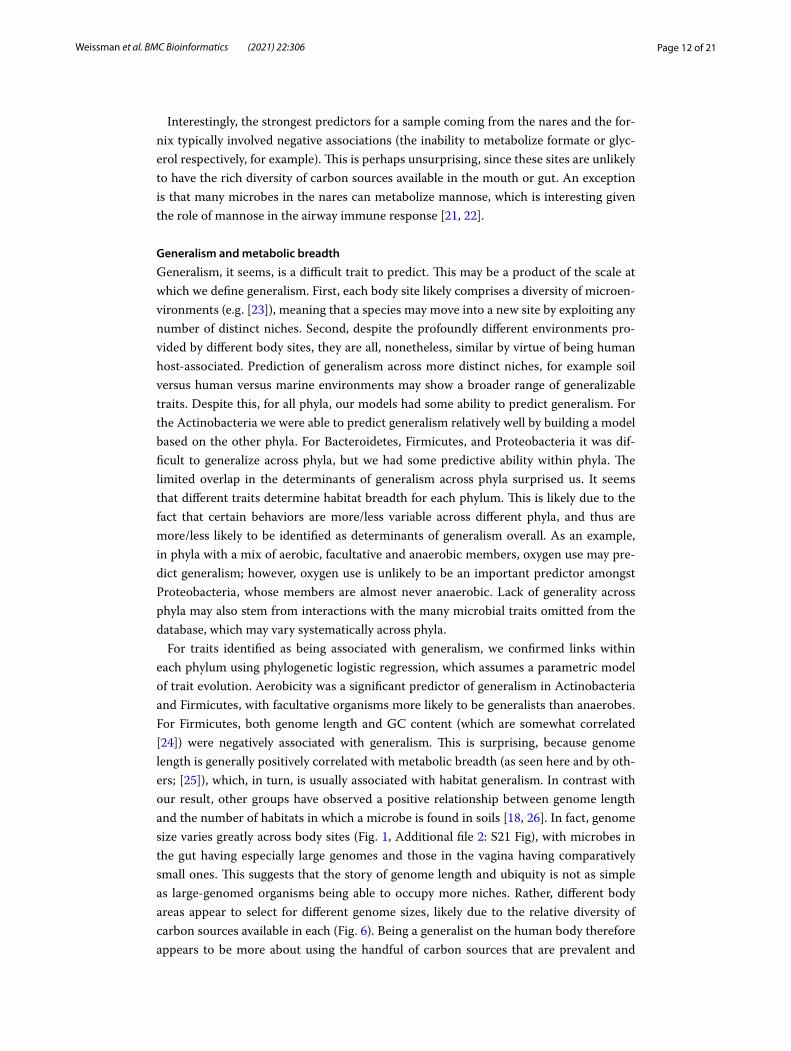
Page 12 of 21Weissman et al. BMC Bioinformatics (2021) 22:306
Interestingly, the strongest predictors for a sample coming from the nares and the for-nix typically involved negative associations (the inability to metabolize formate or glyc-erol respectively, for example). This is perhaps unsurprising, since these sites are unlikely to have the rich diversity of carbon sources available in the mouth or gut. An exception is that many microbes in the nares can metabolize mannose, which is interesting given the role of mannose in the airway immune response [21, 22].
Generalism and metabolic breadth
Generalism, it seems, is a difficult trait to predict. This may be a product of the scale at which we define generalism. First, each body site likely comprises a diversity of microen-vironments (e.g. [23]), meaning that a species may move into a new site by exploiting any number of distinct niches. Second, despite the profoundly different environments pro-vided by different body sites, they are all, nonetheless, similar by virtue of being human host-associated. Prediction of generalism across more distinct niches, for example soil versus human versus marine environments may show a broader range of generalizable traits. Despite this, for all phyla, our models had some ability to predict generalism. For the Actinobacteria we were able to predict generalism relatively well by building a model based on the other phyla. For Bacteroidetes, Firmicutes, and Proteobacteria it was dif-ficult to generalize across phyla, but we had some predictive ability within phyla. The limited overlap in the determinants of generalism across phyla surprised us. It seems that different traits determine habitat breadth for each phylum. This is likely due to the fact that certain behaviors are more/less variable across different phyla, and thus are more/less likely to be identified as determinants of generalism overall. As an example, in phyla with a mix of aerobic, facultative and anaerobic members, oxygen use may pre-dict generalism; however, oxygen use is unlikely to be an important predictor amongst Proteobacteria, whose members are almost never anaerobic. Lack of generality across phyla may also stem from interactions with the many microbial traits omitted from the database, which may vary systematically across phyla.
For traits identified as being associated with generalism, we confirmed links within each phylum using phylogenetic logistic regression, which assumes a parametric model of trait evolution. Aerobicity was a significant predictor of generalism in Actinobacteria and Firmicutes, with facultative organisms more likely to be generalists than anaerobes. For Firmicutes, both genome length and GC content (which are somewhat correlated [24]) were negatively associated with generalism. This is surprising, because genome length is generally positively correlated with metabolic breadth (as seen here and by oth-ers; [25]), which, in turn, is usually associated with habitat generalism. In contrast with our result, other groups have observed a positive relationship between genome length and the number of habitats in which a microbe is found in soils [18, 26]. In fact, genome size varies greatly across body sites (Fig. 1, Additional file 2: S21 Fig), with microbes in the gut having especially large genomes and those in the vagina having comparatively small ones. This suggests that the story of genome length and ubiquity is not as simple as large-genomed organisms being able to occupy more niches. Rather, different body areas appear to select for different genome sizes, likely due to the relative diversity of carbon sources available in each (Fig. 6). Being a generalist on the human body therefore appears to be more about using the handful of carbon sources that are prevalent and
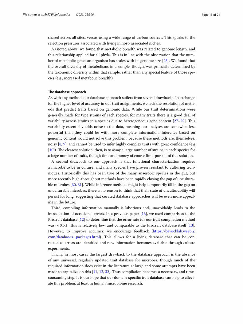
Page 13 of 21Weissman et al. BMC Bioinformatics (2021) 22:306
shared across all sites, versus using a wide range of carbon sources. This speaks to the selection pressures associated with living in host- associated niches.
As noted above, we found that metabolic breadth was related to genome length, and this relationship applied for all phyla. This is in line with the observation that the num-ber of metabolic genes an organism has scales with its genome size [25]. We found that the overall diversity of metabolisms in a sample, though, was primarily determined by the taxonomic diversity within that sample, rather than any special feature of those spe-cies (e.g., increased metabolic breadth).
The database approach
As with any method, our database approach suffers from several drawbacks. In exchange for the higher level of accuracy in our trait assignments, we lack the resolution of meth-ods that predict traits based on genomic data. While our trait determinations were generally made for type strains of each species, for many traits there is a good deal of variability across strains in a species due to heterogeneous gene content [27–29]. This variability essentially adds noise to the data, meaning our analyses are somewhat less powerful than they could be with more complete information. Inference based on genomic content would not solve this problem, because these methods are, themselves, noisy [8, 9], and cannot be used to infer highly complex traits with great confidence (e.g [10]). The clearest solution, then, is to assay a large number of strains in each species for a large number of traits, though time and money of course limit pursuit of this solution.
A second drawback to our approach is that functional characterization requires a microbe to be in culture, and many species have proven resistant to culturing tech-niques. Historically this has been true of the many anaerobic species in the gut, but more recently high-throughput methods have been rapidly closing the gap of uncultura-ble microbes [30, 31]. While inference methods might help temporarily fill in the gap on unculturable microbes, there is no reason to think that their state of unculturability will persist for long, suggesting that curated database approaches will be even more appeal-ing in the future.
Third, compiling information manually is laborious and, unavoidably, leads to the introduction of occasional errors. In a previous paper [13], we used comparison to the ProTrait database [12] to determine that the error rate for our trait compilation method was ∼ 0.5% . This is relatively low, and comparable to the ProTrait database itself [13]. However, to improve accuracy, we encourage feedback (https:// bewic klab. weebly. com/ datab ases-- packa ges. html). This allows for a living database that can be cor-rected as errors are identified and new information becomes available through culture experiments.
Finally, in most cases the largest drawback to the database approach is the absence of any universal, regularly updated trait database for microbes, though much of the required information does exist in the literature at large and some attempts have been made to capitalize on this [11, 12, 32]. Thus compilation becomes a necessary, and time-consuming step. It is our hope that our domain-specific trait database can help to allevi-ate this problem, at least in human microbiome research.
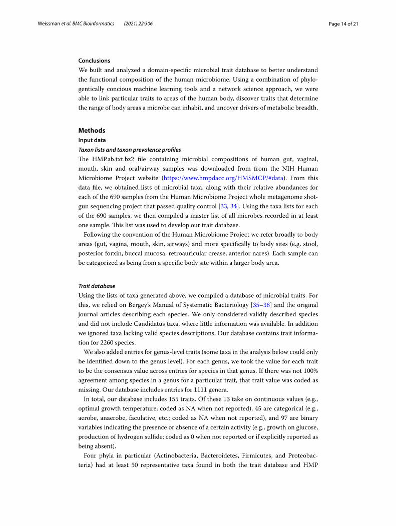
Page 14 of 21Weissman et al. BMC Bioinformatics (2021) 22:306
Conclusions
We built and analyzed a domain-specific microbial trait database to better understand the functional composition of the human microbiome. Using a combination of phylo-gentically concious machine learning tools and a network science approach, we were able to link particular traits to areas of the human body, discover traits that determine the range of body areas a microbe can inhabit, and uncover drivers of metabolic breadth.
MethodsInput data
Taxon lists and taxon prevalence profiles
The HMP.ab.txt.bz2 file containing microbial compositions of human gut, vaginal, mouth, skin and oral/airway samples was downloaded from from the NIH Human Microbiome Project website (https:// www. hmpda cc. org/ HMSMC P/# data). From this data file, we obtained lists of microbial taxa, along with their relative abundances for each of the 690 samples from the Human Microbiome Project whole metagenome shot-gun sequencing project that passed quality control [33, 34]. Using the taxa lists for each of the 690 samples, we then compiled a master list of all microbes recorded in at least one sample. This list was used to develop our trait database.
Following the convention of the Human Microbiome Project we refer broadly to body areas (gut, vagina, mouth, skin, airways) and more specifically to body sites (e.g. stool, posterior forxin, buccal mucosa, retroauricular crease, anterior nares). Each sample can be categorized as being from a specific body site within a larger body area.
Trait database
Using the lists of taxa generated above, we compiled a database of microbial traits. For this, we relied on Bergey’s Manual of Systematic Bacteriology [35–38] and the original journal articles describing each species. We only considered validly described species and did not include Candidatus taxa, where little information was available. In addition we ignored taxa lacking valid species descriptions. Our database contains trait informa-tion for 2260 species.
We also added entries for genus-level traits (some taxa in the analysis below could only be identified down to the genus level). For each genus, we took the value for each trait to be the consensus value across entries for species in that genus. If there was not 100% agreement among species in a genus for a particular trait, that trait value was coded as missing. Our database includes entries for 1111 genera.
In total, our database includes 155 traits. Of these 13 take on continuous values (e.g., optimal growth temperature; coded as NA when not reported), 45 are categorical (e.g., aerobe, anaerobe, faculative, etc.; coded as NA when not reported), and 97 are binary variables indicating the presence or absence of a certain activity (e.g., growth on glucose, production of hydrogen sulfide; coded as 0 when not reported or if explicitly reported as being absent).
Four phyla in particular (Actinobacteria, Bacteroidetes, Firmicutes, and Proteobac-teria) had at least 50 representative taxa found in both the trait database and HMP
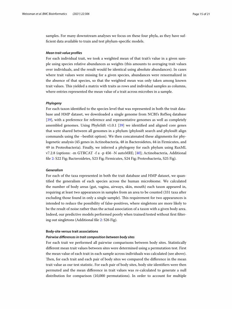
Page 15 of 21Weissman et al. BMC Bioinformatics (2021) 22:306
samples. For many downstream analyses we focus on these four phyla, as they have suf-ficient data available to train and test phylum-specific models.
Mean trait value profiles
For each individual trait, we took a weighted mean of that trait’s value in a given sam-ple using species relative abundances as weights (this amounts to averaging trait values over individuals, and the result would be identical using absolute abundances). In cases where trait values were missing for a given species, abundances were renormalized in the absence of that species, so that the weighted mean was only taken among known trait values. This yielded a matrix with traits as rows and individual samples as columns, where entries represented the mean value of a trait across microbes in a sample.
Phylogeny
For each taxon identified to the species level that was represented in both the trait data-base and HMP dataset, we downloaded a single genome from NCBI’s RefSeq database [39], with a preference for reference and representative genomes as well as completely assembled genomes. Using PhyloSift v1.0.1 [39] we identified and aligned core genes that were shared between all genomes in a phylum (phylosift search and phylosift align commands using the –besthit option). We then concatenated these alignments for phy-logenetic analysis (45 genes in Actinobacteria, 48 in Bacteroidetes, 44 in Firmicutes, and 49 in Proteobacteria). Finally, we inferred a phylogeny for each phylum using RaxML v7.2.8 (options: -m GTR CAT -f a -p 456 -N autoMRE; [40]; Actinobacteria, Additional file 2: S22 Fig; Bacteroidetes, S23 Fig; Firmicutes, S24 Fig; Proteobacteria, S25 Fig).
Generalism
For each of the taxa represented in both the trait database and HMP dataset, we quan-tified the generalism of each species across the human microbiome. We calculated the number of body areas (gut, vagina, airways, skin, mouth) each taxon appeared in, requiring at least two appearances in samples from an area to be counted (331 taxa after excluding those found in only a single sample). This requirement for two appearances is intended to reduce the possibility of false-positives, where singletons are more likely to be the result of noise rather than the actual association of a taxon with a given body area. Indeed, our predictive models performed poorly when trained/tested without first filter-ing out singletons (Additional file 2: S26 Fig).
Body‑site versus trait associations
Pairwise differences in trait composition between body sites
For each trait we performed all pairwise comparisons between body sites. Statistically different mean trait values between sites were determined using a permutation test. First the mean value of each trait in each sample across individuals was calculated (see above). Then, for each trait and each pair of body sites we compared the difference in the mean trait value as our test statistic. For each pair of body sites, body site identifiers were then permuted and the mean difference in trait values was re-calculated to generate a null distribution for comparison (10,000 permutations). In order to account for multiple
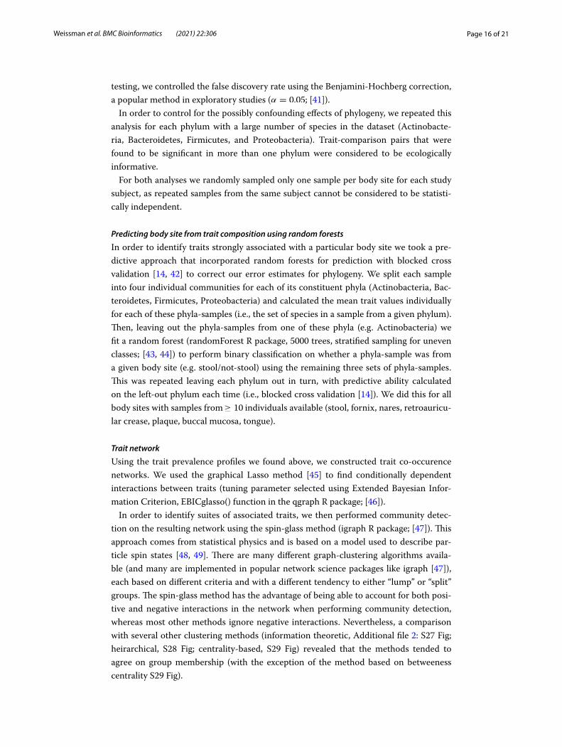
Page 16 of 21Weissman et al. BMC Bioinformatics (2021) 22:306
testing, we controlled the false discovery rate using the Benjamini-Hochberg correction, a popular method in exploratory studies ( α = 0.05 ; [41]).
In order to control for the possibly confounding effects of phylogeny, we repeated this analysis for each phylum with a large number of species in the dataset (Actinobacte-ria, Bacteroidetes, Firmicutes, and Proteobacteria). Trait-comparison pairs that were found to be significant in more than one phylum were considered to be ecologically informative.
For both analyses we randomly sampled only one sample per body site for each study subject, as repeated samples from the same subject cannot be considered to be statisti-cally independent.
Predicting body site from trait composition using random forests
In order to identify traits strongly associated with a particular body site we took a pre-dictive approach that incorporated random forests for prediction with blocked cross validation [14, 42] to correct our error estimates for phylogeny. We split each sample into four individual communities for each of its constituent phyla (Actinobacteria, Bac-teroidetes, Firmicutes, Proteobacteria) and calculated the mean trait values individually for each of these phyla-samples (i.e., the set of species in a sample from a given phylum). Then, leaving out the phyla-samples from one of these phyla (e.g. Actinobacteria) we fit a random forest (randomForest R package, 5000 trees, stratified sampling for uneven classes; [43, 44]) to perform binary classification on whether a phyla-sample was from a given body site (e.g. stool/not-stool) using the remaining three sets of phyla-samples. This was repeated leaving each phylum out in turn, with predictive ability calculated on the left-out phylum each time (i.e., blocked cross validation [14]). We did this for all body sites with samples from ≥ 10 individuals available (stool, fornix, nares, retroauricu-lar crease, plaque, buccal mucosa, tongue).
Trait network
Using the trait prevalence profiles we found above, we constructed trait co-occurence networks. We used the graphical Lasso method [45] to find conditionally dependent interactions between traits (tuning parameter selected using Extended Bayesian Infor-mation Criterion, EBICglasso() function in the qgraph R package; [46]).
In order to identify suites of associated traits, we then performed community detec-tion on the resulting network using the spin-glass method (igraph R package; [47]). This approach comes from statistical physics and is based on a model used to describe par-ticle spin states [48, 49]. There are many different graph-clustering algorithms availa-ble (and many are implemented in popular network science packages like igraph [47]), each based on different criteria and with a different tendency to either “lump” or “split” groups. The spin-glass method has the advantage of being able to account for both posi-tive and negative interactions in the network when performing community detection, whereas most other methods ignore negative interactions. Nevertheless, a comparison with several other clustering methods (information theoretic, Additional file 2: S27 Fig; heirarchical, S28 Fig; centrality-based, S29 Fig) revealed that the methods tended to agree on group membership (with the exception of the method based on betweeness centrality S29 Fig).

Page 17 of 21Weissman et al. BMC Bioinformatics (2021) 22:306
We then built a bipartite network associating the trait clusters we found above with specific body sites. We performed Lasso regressions with each site as a binary outcome variable (glmnet package in R, 10-fold cross validation on mis-classification error to choose � ; [50]) and the trait values associated with that site as predictors. We then took the weight of an edge connecting each site with each cluster as the mean regression coef-ficient for a site with all traits in a given cluster that were retained in the model.
Predicting generalism using random forests
We constructed random forest models to predict generalism within each phylum (ran-domForest R package, 5000 trees, stratified sampling for uneven classes). For simplicity, we coded specialism/generalism as binary trait, where a species was considered a spe-cialist if it appeared in one body area only, and a generalist if it appeared in more than one body area. Any missing trait values for a given taxon were imputed using the mean trait value in the database. The out-of-bag error estimate produced during the fitting of a random forest will give a biased estimate of model performance when observations are not independent of one another. This is potentially the case for our phylogenetically structured dataset. To get an accurate estimate of our prediction error we used blocked cross validation [14], in which, instead of choosing folds at random from the data, we choose monophyletic clades on the phylogeny. By estimating our error on groups that can be considered to have evolved independently of the data on which the model was trained, we prevented confounding the effects of phylogenetic structure from influenc-ing our model accuracy estimates.
In practice this meant building a series of random forest models for a given phylogeny, each leaving out a single class (blocked cross validation with classes as the folds). We then estimated our error by predicting each of the excluded folds in turn and calculating metrics of model performance. We repeated this process for each phylum.
To assess how well we could predict generalism when extrapolating across phyla (as opposed to within phyla, as above), we took a similar approach, this time considering all phyla together in a blocked cross validation framework, and using each phylum as a fold. We then assessed cross-phylum performance by predicting the generalism of species in one phylum using a model trained on the three other phyla, repeating for each phylum in turn.
Phylogenetic logistic regression to test for significant associations
We followed up our random forest analysis of generalism with a formal correction for phylogeny. We obtained the most important traits that predicted generalism by build-ing a random forest on each phylum individually, and then selecting the top five ranked traits for each model based on mean decrease in the accuracy of the model when that variable’s values are permuted. We then performed phylogenetic logistic regression to predict generalism based on each of these traits for each of the relevant phyla (20 tests, phylolm R package; [51]). Following the recommendation of Ives and Garland based on our small sample size [52], we report bootstrapped p values (10,000 bootstraps).

Page 18 of 21Weissman et al. BMC Bioinformatics (2021) 22:306
Metabolic breadth versus trait associations
We predicted metabolic breadth of taxa using a similar approach to that used for prediction of generalism. Specifically, we defined metabolic breadth of a taxon as the number of carbon substrates on which a microbe can grow as recorded in our data-base. We then attempted to predict this number using all other traits (excluding sub-strate use traits). We used a blocked-cross validation approach with phyla as folds, and built random forests for regression (randomForest R package, 5000 trees).
Model assessment
We used Cohen’s κ [53] as our index of model performance. Briefly, this index meas-ures the increase in predictive performance over a null model that has information only about class prevalence. If classes are highly unbalanced, it is easy to acheive high accuracy with little discriminative ability by always guessing the prevalent class. Cohen’s κ essentially corrects for this problem. Values greater than zero indicate dis-criminative ability greater than this null model, whereas negative values indicate the opposite (e.g., randomly guessing “yes” 50% of the time when the actual prevalence is “yes” 90% of the time). As noted above, in order to get an unbiased/phylogenetically corrected estimate of model performance we used blocked-cross validation, predict-ing the quantity of interest (source site, generalism, metabolic breadth, etc.) for each phylum in turn on the basis of the others and taking the mean κ across these models.
AbbreviationspH: Potential of hydrogen; FDR: False discovery rate; RMSE: Root mean squared error; NCBI: National Center for Biotech-nology Information; HMP: Human Microbiome Project; EBIC: Extended Bayesian information criterion.
Supplementary InformationThe online version contains supplementary material available at https:// doi. org/ 10. 1186/ s12859- 021- 04216-2.
Additional file 1. Trait Database.
Additional file 2. Supplemental Table and Figures.
AcknowledgementsNot applicable.
Authors’ contributionsJW, SB, DK and WF conceived of the paper, and SB oversaw trait database generation. JW, PJ, PT, and FB performed bioin-formatics and statistical analyses. Each of SD, KJ, SB, RF, CD, JB, KD, TP, and SA entered data on over 200 organisms. JW, SB, and WF wrote the paper. All authors have read and approved the manuscript.
FundingThis work was support by the U.S. Army Research Laboratory and the U.S. Army Research Office under contract/Grant Number #W911NF-14-1-0490 (JW, DK, WFF, PT, FB, and SB). JW was supported in part by NSF award DGE-1632976.
Availability of data and materialsAll data generated or analysed during this study are included in this published article.
Declarations
Ethics approval and consent to participateNot applicable.
Consent for publicationNot applicable.

Page 19 of 21Weissman et al. BMC Bioinformatics (2021) 22:306
Competing interestsThe authors declare that they have no competing interests.
Author details1 Department of Biology, University of Maryland - College Park, College Park, MD, USA. 2 Research and Exploratory Development Department, Johns Hopkins Applied Physics Laboratory, Laurel, MD, USA. 3 Bioengineering Department, Clemson University, Clemson, SC, USA. 4 Biological Sciences Department, Clemson University, Clemson, SC, USA.
Received: 3 November 2019 Accepted: 25 May 2021
References 1. Cho I, Blaser MJ. The human microbiome: at the interface of health and disease. Nat Rev Genet. 2012;13(4):260–70.
https:// doi. org/ 10. 1038/ nrg31 82. 2. Heijden MGAVD, Bardgett RD, Straalen NMV. The unseen majority: soil microbes as drivers of plant diversity and pro-
ductivity in terrestrial ecosystems. Ecol Lett. 2008;11(3):296–310. https:// doi. org/ 10. 1111/j. 1461- 0248. 2007. 01139.x. 3. Bardgett RD, Freeman C, Ostle NJ. Microbial contributions to climate change through carbon cycle feedbacks. ISME
J. 2008;2(8):805–14. https:// doi. org/ 10. 1038/ ismej. 2008. 58. 4. Shafquat A, Joice R, Simmons SL, Huttenhower C. Functional and phylogenetic assembly of microbial communities
in the human microbiome. Trends Microbiol. 2014;22(5):261–6. https:// doi. org/ 10. 1016/j. tim. 2014. 01. 011. 5. Louca S, Jacques SMS, Pires APF, Leal JS, Srivastava DS, Parfrey LW, Farjalla VF, Doebeli M. High taxonomic variability
despite stable functional structure across microbial communities. Nat Ecol Evolut. 2017;1(1):0015. https:// doi. org/ 10. 1038/ s41559- 016- 0015.
6. Louca S, Polz MF, Mazel F, Albright MBN, Huber JA, O’Connor MI, Ackermann M, Hahn AS, Srivastava DS, Crowe SA, Doebeli M, Parfrey LW. Function and functional redundancy in microbial systems. Nat Ecol Evolut. 2018;2(6):936. https:// doi. org/ 10. 1038/ s41559- 018- 0519-1.
7. Abubucker S, Segata N, Goll J, Schubert AM, Izard J, Cantarel BL, Rodriguez-Mueller B, Zucker J, Thiagarajan M, Henrissat B, White O, Kelley ST, Methé B, Schloss PD, Gevers D, Mitreva M, Huttenhower C. Metabolic reconstruction for metagenomic data and its application to the human microbiome. PLoS Comput Biol. 2012;8(6):1002358. https:// doi. org/ 10. 1371/ journ al. pcbi. 10023 58.
8. Plata G, Henry CS, Vitkup D. Long-term phenotypic evolution of bacteria. Nature. 2015;517(7534):369–72. https:// doi. org/ 10. 1038/ natur e13827.
9. Henry CS, DeJongh M, Best AA, Frybarger PM, Linsay B, Stevens RL. High-throughput generation, optimization and analysis of genome-scale metabolic models. Nat Biotechnol. 2010;28(9):977–82. https:// doi. org/ 10. 1038/ nbt. 1672.
10. Jensen DB, Ussery DW. Bayesian prediction of microbial oxygen requirement. F1000Research. 2013. https:// doi. org/ 10. 12688/ f1000 resea rch.2- 184. v1.
11. Barberán A, Velazquez HC, Jones S, Fierer N. Hiding in plain sight: mining bacterial species records for phenotypic trait information. mSphere. 2017;2(4):00237–17. https:// doi. org/ 10. 1128/ mSphe re. 00237- 17.
12. Brbić M, Piškorec M, Vidulin V, Kriško A, Šmuc T, Supek F. The landscape of microbial phenotypic traits and associated genes. Nucleic Acids Res. 2016;44(21):10074–90. https:// doi. org/ 10. 1093/ nar/ gkw964.
13. Bewick S, Gurarie E, Weissman JL, Beattie J, Davati C, Flint R, Thielen P, Breitwieser F, Karig D, Fagan WF. Trait-based analysis of the human skin microbiome. Microbiome. 2019;7(1):1–15.
14. Roberts DR, Bahn V, Ciuti S, Boyce MS, Elith J, Guillera-Arroita G, Hauenstein S, Lahoz-Monfort JJ, Schröder B, Thuiller W, Warton DI, Wintle BA, Hartig F, Dormann CF. Cross-validation strategies for data with temporal, spatial, hierarchi-cal, or phylogenetic structure. Ecography. 2017;40(8):913–29. https:// doi. org/ 10. 1111/ ecog. 02881.
15. The Human Microbiome Project Consortium, Huttenhower C, Gevers D, Knight R, Abubucker S, Badger JH, Chin-walla AT, Creasy HH, Earl AM, FitzGerald MG, Fulton RS, Giglio MG, Hallsworth-Pepin K, Lobos EA, Madupu R, Magrini V, Martin JC, Mitreva M, Muzny DM, Sodergren EJ, Versalovic J, Wollam AM, Worley KC, Wortman JR, Young SK, Zeng Q, Aagaard KM, Abolude OO, Allen-Vercoe E, Alm EJ, Alvarado L, Andersen GL, Anderson S, Appelbaum E, Arachchi HM, Armitage G, Arze CA, Ayvaz T, Baker CC, Begg L, Belachew T, Bhonagiri V, Bihan M, Blaser MJ, Bloom T, Bonazzi V, Paul Brooks J, Buck GA, Buhay CJ, Busam DA, Campbell JL, Canon SR, Cantarel BL, Chain PSG, Chen I-MA, Chen L, Chhibba S, Chu K, Ciulla DM, Clemente JC, Clifton SW, Conlan S, Crabtree J, Cutting MA, Davidovics NJ, Davis CC, DeSantis TZ, Deal C, Delehaunty KD, Dewhirst FE, Deych E, Ding Y, Dooling DJ, Dugan SP, Michael Dunne W, Scott Durkin A, Edgar RC, Erlich RL, Farmer CN, Farrell RM, Faust K, Feldgarden M, Felix VM, Fisher S, Fodor AA, Forney LJ, Foster L, Di Francesco V, Friedman J, Friedrich DC, Fronick CC, Fulton LL, Gao H, Garcia N, Giannoukos G, Giblin C, Giovanni MY, Goldberg JM, Goll J, Gonzalez A, Griggs A, Gujja S, Kinder Haake S, Haas BJ, Hamilton HA, Harris EL, Hepburn TA, Herter B, Hoffmann DE, Holder ME, Howarth C, Huang KH, Huse SM, Izard J, Jansson JK, Jiang H, Jordan C, Joshi V, Katancik, JA Keitel, WA Kelley ST, Kells C, King NB, Knights D, Kong HH, Koren O, Koren S, Kota KC, Kovar CL, Kyrpides NC, La Rosa PS, Lee SL, Lemon KP, Lennon N, Lewis CM, Lewis L, Ley RE, Li K, Liolios K, Liu B, Liu Y, Lo C-C, Lozupone CA, Dwayne Lunsford R, Madden T, Mahurkar AA, Mannon PJ, Mardis ER, Markowitz VM, Mavromatis K, McCorrison JM, McDonald D, McEwen J, McGuire AL, McInnes P, Mehta T, Mihindukulasuriya KA, Miller JR, Minx PJ, Newsham I, Nusbaum C, O’Laughlin M, Orvis J, Pagani I, Palaniappan K, Patel SM, Pearson M, Peterson J, Podar M, Pohl C, Pollard KS, Pop M, Priest ME, Proctor LM, Qin X, Raes J, Ravel J, Reid JG, Rho M, Rhodes R, Riehle KP, Rivera MC, Rodriguez-Mueller B, Rogers Y-H, Ross MC, Russ C, Sanka RK, Sankar P, Fah Sathirapongsasuti J, Schloss JA, Schloss PD, Schmidt TM, Scholz M, Schriml L, Schubert AM, Segata N, Segre JA, Shannon WD, Sharp RR, Sharpton TJ, Shenoy

Page 20 of 21Weissman et al. BMC Bioinformatics (2021) 22:306
N, Sheth NU, Simone GA, Singh I, Smillie CS, Sobel JD, Sommer DD, Spicer P, Sutton GG, Sykes SM, Tabbaa DG, Thia-garajan M, Tomlinson CM, Torralba M, Treangen TJ, Truty RM, Vishnivetskaya TA, Walker J, Wang L, Wang Z, Ward DV, Warren W, Watson MA, Wellington C, Wetterstrand KA, White JR, Wilczek-Boney K, Wu Y, Wylie KM, Wylie T, Yandava C, Ye L, Ye Y, Yooseph S, Youmans BP, Zhang L, Zhou Y, Zhu Y, Zoloth L, Zucker JD, Birren BW, Gibbs RA, Highlander SK, Methé BA, Nelson KE, Petrosino JF, Weinstock GM, Wilson RK, White O Structure, function and diversity of the healthy human microbiome. Nature 2012;486(7402):207–214 https:// doi. org/ 10. 1038/ natur e11234.
16. Shin N-R, Whon TW, Bae J-W. Proteobacteria: microbial signature of dysbiosis in gut microbiota. Trends Biotechnol. 2015;33(9):496–503. https:// doi. org/ 10. 1016/j. tibte ch. 2015. 06. 011.
17. Allaband C, McDonald D, Vázquez-Baeza Y, Minich JJ, Tripathi A, Brenner DA, Loomba R, Smarr L, Sandborn WJ, Schnabl B, et al. Microbiome 101: studying, analyzing, and interpreting gut microbiome data for clinicians. Clin Gastroenterol Hepatol. 2019;17(2):218–30.
18. Barberán A, Ramirez KS, Leff JW, Bradford MA, Wall DH, Fierer N. Why are some microbes more ubiquitous than oth-ers? Predicting the habitat breadth of soil bacteria. Ecol Lett. 2014;17(7):794–802. https:// doi. org/ 10. 1111/ ele. 12282.
19. Andersson S, Nilsson SI. Influence of ph and temperature on microbial activity, substrate availability of soil-solution bacteria and leaching of dissolved organic carbon in a mor humus. Soil Biol Biochem. 2001;33(9):1181–91.
20. Land M, Hauser L, Jun S-R, Nookaew I, Leuze MR, Ahn T-H, Karpinets T, Lund O, Kora G, Wassenaar T, et al. Insights from 20 years of bacterial genome sequencing. Funct Integr Genom. 2015;15(2):141–61.
21. Casanova J-L, Abel L. Human mannose-binding lectin in immunity: friend, foe, or both? J Exp Med. 2004;199(10):1295–9.
22. Fidler KJ, Hilliard TN, Bush A, Johnson M, Geddes DM, Turner MW, Alton EW, Klein NJ, Davies JC. Mannose-binding lectin is present in the infected airway: a possible pulmonary defence mechanism. Thorax. 2009;64(2):150–5.
23. De Weirdt R, Van de Wiele T. Micromanagement in the gut: microenvironmental factors govern colon mucosal bio-film structure and functionality. NPJ Biofilms Microbiomes. 2015;1:15026. https:// doi. org/ 10. 1038/ npjbi ofilms. 2015. 26.
24. Almpanis A, Swain M, Gatherer D, McEwan N. Correlation between bacterial G+C content, genome size and the G+C content of associated plasmids and bacteriophages. Microbial Genom. 2018;4(4):e000168.
25. Konstantinidis KT, Tiedje JM. Trends between gene content and genome size in prokaryotic species with larger genomes. Proc Nat Acad Sci. 2004;101(9):3160–5. https:// doi. org/ 10. 1073/ pnas. 03086 53100.
26. Cobo-Simón M, Tamames J. Relating genomic characteristics to environmental preferences and ubiquity in different microbial taxa. BMC Genom. 2017;18(1):499. https:// doi. org/ 10. 1186/ s12864- 017- 3888-y.
27. Konstantinidis KT, Tiedje JM. Genomic insights that advance the species definition for prokaryotes. Proc Nat Acad Sci USA. 2005;102(7):2567–72. https:// doi. org/ 10. 1073/ pnas. 04097 27102.
28. Doolittle WF, Papke RT. Genomics and the bacterial species problem. Genome Biol. 2006;7(9):116. https:// doi. org/ 10. 1186/ gb- 2006-7- 9- 116.
29. Zhu A, Sunagawa S, Mende DR, Bork P. Inter-individual differences in the gene content of human gut bacterial spe-cies. Genome Biol. 2015. https:// doi. org/ 10. 1186/ s13059- 015- 0646-9.
30. Lagier J-C, Khelaifia S, Alou MT, Ndongo S, Dione N, Hugon P, Caputo A, Cadoret F, Traore SI, Seck EH, Dubourg G, Durand G, Mourembou G, Guilhot E, Togo A, Bellali S, Bachar D, Cassir N, Bittar F, Delerce J, Mailhe M, Ricaboni D, Bilen M, Dangui Nieko NPM, DiaBadiane NM, Valles C, Mouelhi D, Diop K, Million M, Musso D, Abrahão J, Azhar EI, Bibi F, Yasir M, Diallo A, Sokhna C, Djossou F, Vitton V, Robert C, Rolain JM, La Scola B, Fournier P-E, Levasseur A, Raoult D. Culture of previously uncultured members of the human gut microbiota by culturomics. Nat Microbiol. 2016;1(12):16203. https:// doi. org/ 10. 1038/ nmicr obiol. 2016. 203.
31. Browne HP, Forster SC, Anonye BO, Kumar N, Neville BA, Stares MD, Goulding D, Lawley TD. Culturing of ‘uncultur-able’ human microbiota reveals novel taxa and extensive sporulation. Nature. 2016;533(7604):543–6. https:// doi. org/ 10. 1038/ natur e17645.
32. Madin JS, Nielsen DA, Brbic M, Corkrey R, Danko D, Edwards K, Engqvist MK, Fierer N, Geoghegan JL, Gillings M, et al. A synthesis of bacterial and archaeal phenotypic trait data. Sci Data. 2020;7(1):1–8.
33. Huttenhower C, Gevers D, Knight R, Abubucker S, Badger JH, Chinwalla AT, Creasy HH, Earl AM, FitzGerald MG, Fulton RS, et al. Structure, function and diversity of the healthy human microbiome. Nature. 2012;486(7402):207.
34. Methé BA, Nelson KE, Pop M, Creasy HH, Giglio MG, Huttenhower C, Gevers D, Petrosino JF, Abubucker S, Badger JH, et al. A framework for human microbiome research. Nature. 2012;486(7402):215.
35. Garrity G, Staley JT, Boone DR, De Vos P, Goodfellow M, Rainey FA, Garrity GM, Schleifer K-H. Bergey’s Manual® of Systematic Bacteriology: Volume Two: The Proteobacteria. Springer, Berlin; 2006.
36. Vos P, Garrity G, Jones D, Krieg NR, Ludwig W, Rainey FA, Schleifer K-H, Whitman WB. Bergey’s Manual of Systematic Bacteriology: Volume 3: The Firmicutes vol. 3. Springer, Berlin; 2011.
37. Bergey DBH, Garrity GM, Boone DR, Brenner DJ, Castenholz RW, Goodfellow M, Krieg NR, Staley JT, De Vos P. “Bergey’s Manual of Systematic Bacteriology: Volume 4: The Bacteroidetes, Spirochaetes, Tenericutes (Mollicutes), Acidobacteria, Fibrobacteres, Fusobacteria, Dictyoglomi, Gemmatimonadetes, Lentisphaerae, Verrucomicrobia, Chlamydiae, and Planc-tomycetes” Berlin: Springer; 2011.
38. Goodfellow M, Kämpfer P, Busse H-J, Trujillo ME, Suzuki K-i, Ludwig W, Whitman WB. Bergey’s Manual® of systematic bacteriology: volume five the actinobacteria, part A. Springer, Berlin; 2012.
39. Haft DH, DiCuccio M, Badretdin A, Brover V, Chetvernin V, O’Neill K, Li W, Chitsaz F, Derbyshire MK, Gonzales NR, Gwadz M, Lu F, Marchler GH, Song JS, Thanki N, Yamashita RA, Zheng C, Thibaud-Nissen F, Geer LY, Marchler-Bauer A, Pruitt KD. RefSeq: an update on prokaryotic genome annotation and curation. Nucleic Acids Res. 2018;46(D1):851–60. https:// doi. org/ 10. 1093/ nar/ gkx10 68.
40. Stamatakis A. RAxML version 8: a tool for phylogenetic analysis and post-analysis of large phylogenies. Bioinformat-ics. 2014;30(9):1312–3. https:// doi. org/ 10. 1093/ bioin forma tics/ btu033.
41. Benjamini Y, Hochberg Y. Controlling the false discovery rate: a practical and powerful approach to multiple testing. J Roy Stat Soc Ser B (Methodol). 1995;57(1):289–300.

Page 21 of 21Weissman et al. BMC Bioinformatics (2021) 22:306
• fast, convenient online submission
•
thorough peer review by experienced researchers in your field
• rapid publication on acceptance
• support for research data, including large and complex data types
•
gold Open Access which fosters wider collaboration and increased citations
maximum visibility for your research: over 100M website views per year •
At BMC, research is always in progress.
Learn more biomedcentral.com/submissions
Ready to submit your researchReady to submit your research ? Choose BMC and benefit from: ? Choose BMC and benefit from:
42. Weissman JL, Laljani R, Fagan WF, Johnson PLF. Ecology shapes microbial immune strategy: temperature and oxy-gen as determinants of the incidence of CRISPR adaptive immunity. bioRxiv, 326330; 2018. https:// doi. org/ 10. 1101/ 326330.
43. Breiman L. Random forests. Mach Learn. 2001;45(1):5–32. https:// doi. org/ 10. 1023/A: 10109 33404 324. 44. Liaw A, Wiener M. Classification and regression by randomForest. R News. 2002;2(3):18–22. 45. Friedman J, Hastie T, Tibshirani R. Sparse inverse covariance estimation with the graphical lasso. Biostatistics (Oxford,
England). 2008;9(3):432–41. https:// doi. org/ 10. 1093/ biost atist ics/ kxm045. 46. Epskamp S, Cramer AOJ, Waldorp LJ, Schmittmann VD, Borsboom D. qgraph: Network visualizations of relationships
in psychometric data. J Stat Softw. 2012;48(1):1–18. https:// doi. org/ 10. 18637/ jss. v048. i04. 47. Csardi G, Nepusz T. The igraph software package for complex network research. InterJournal Complex Systems.
2006;1695. 48. Reichardt J, Bornholdt S. Statistical mechanics of community detection. Phys Rev E. 2006. https:// doi. org/ 10. 1103/
PhysR evE. 74. 016110. 49. Traag VA, Bruggeman J. Community detection in networks with positive and negative links. Phys Rev E. 2009.
https:// doi. org/ 10. 1103/ PhysR evE. 80. 036115. 50. Friedman J, Hastie T, Tibshirani R. Regularization paths for generalized linear models via coordinate descent. J Stat
Softw. 2010;33(1):1–22. 51. Ho LST, Ane C. A linear-time algorithm for Gaussian and non-Gaussian trait evolution models. Syst Biol.
2014;63:397–408. 52. Ives AR, Garland T. Phylogenetic logistic regression for binary dependent variables. Syst Biol. 2010;59(1):9–26. https://
doi. org/ 10. 1093/ sysbio/ syp074. 53. Cohen J. A coefficient of agreement for nominal scales. Educ Psychol Meas. 1960;20(1):37–46.
Publisher’s NoteSpringer Nature remains neutral with regard to jurisdictional claims in published maps and institutional affiliations.