exploring link covering and node covering formulations of

Exploring Link Covering and Node Covering Formulations of Detection Layout Problem Authors: J.Barceló1, F. Gilliéron, M.P. Linares1, O. Serch1, L.Montero1

1Department of Statistics and Operations Research and CENIT (Center for Innovation in Transport) Technical University of Catalonia Campus Nord, Building K2M, Office 306 Jordi Girona 29 08034 Barcelona Spain (jaume.barcelo, lidia.montero, mari.paz.linares,oriol.serch)@upc.edu [email protected] Tel: +34 93 405 4659 Paper submitted for presentation and publication to 91st Transportation Research Board 2012 Annual Meeting Washington, D.C. November 2011 # WORDS: 6317 Paper revised from original submittal

mailto:[email protected]

1 Barceló, Guilliéron, Linares, Serch, Montero

ABSTRACT 1 2 The primary data input used in principal traffic models comes from Origin-Destination (OD) 3 trip matrices, which describe the patterns of traffic behavior across the network. In this way, 4 OD matrices become a critical requirement in Advanced Traffic Management and/or 5 Information Systems that are supported by Dynamic Traffic Assignment models. However, 6 because OD matrices are not directly observable, the current practice consists of adjusting an 7 initial or seed matrix from link flow counts which are provided by an existing layout of traffic 8 counting stations. The adequacy of the detection layout strongly determines the quality of the 9 adjusted OD. The usual approaches to the Detection Layout problem assume that detectors are 10 located at network links. The first contribution of this paper proposes a modified set that 11 formulates the link detection layout problem with side constraints. It also presents a new 12 metaheuristic tabu search algorithm with high computational efficiency. The emerging 13 Information and Communication Technologies, especially those based on the detection of the 14 electronic signature of on-board devices (such as Bluetooth devices) allow the location of 15 sensors at intersections. To explicitly take into account how these ICT sensors operate, this 16 paper proposes a new formulation in terms of a node covering problem with side constraints 17 that, for practical purposes, can be efficiently solved with standard professional solvers such 18 as CPLEX. 19 20 Keywords: OD Estimation, Dynamic User Equilibrium, Traffic Detector Location, Link 21 Covering, Node Covering, Integer Programming, Location Theory 22


THE DETECTION LAYOUT PROBLEM 23 24 Traffic detectors are usually the means for measuring fundamental traffic variables (i.e. flows, 25 speeds and occupancies), whose values determine the state of the traffic system. The values of 26 these variables are the main inputs to models based on traffic flow theory for estimating the 27 state of traffic flow at freeway sections, either to study and understand traffic behavior or to 28 support efficient traffic management decisions. These values are also the input to traffic 29 control systems which are used to calculate traffic control plans --be they fixed, actuated or 30 adaptive-- in order to optimize the traffic network. Traffic detectors are usually located along 31 the road in the best positions for achieving these goals. However, when dealing with traffic 32 networks, namely complex urban networks, additional components are necessary for 33 describing and understanding the traffic patterns which account for the behavior of traffic 34 flows in the network. Origin-to-Destination trip matrices describe the number of trips between 35 any origin-destination pair in a traffic network. Route choice models describe how trips select 36 the available paths between origins and destinations and, as a consequence, the number of 37 trips using a given path. In other words, they describe the path flows or the path flow 38 proportions, depending on whether we refer to the number of trips using a path or to the 39 fraction of trips using a path, with respect to the total number of trips between the 40 corresponding origin and destination. 41 42 Traffic assignment models have the objective of assigning a trip matrix onto a network --in 43 terms of a route choice mechanism-- in order to estimate the traffic flows in the network. 44 Therefore, they all use Origin-Destination (OD) trip matrices as major data input for 45 describing the patterns of traffic behavior across the network. All formulations of static traffic 46 assignment models (Florian and Hearn [1], as well as dynamic, Ben-Akiva et al. [2]) assume 47 that a reliable estimate of an OD is available. However, OD matrices are not yet directly 48 observable, even less so in the case of the time-dependent OD matrices that are necessary for 49 Dynamic Traffic Assignment models; consequently, it has been natural to resort to indirect 50 estimation methods. These indirect estimation methods are the so-called matrix adjustment 51 methods, whose main modeling hypothesis can be stated as follows: if traffic flows in the 52 links of a network are the consequence of the assignment of an OD matrix onto a network, 53 then, if we are capable of measuring link flows, the problem of estimating the OD matrix that 54 generates such flows can be considered as the inverse of the assignment problem (Cascetta 55 [3]). Since the earlier formulation of the problem by Van Zuylen and Willumsen [4], the 56 matrix adjustment problem has been a relevant research and practical problem. 57 58 The current practices consist of using an initial OD estimate, the OD seed or OD target as 59 input, and adjusting them from the available link counts provided by an existing layout of 60 traffic counting stations and other additional information whenever it is available. 61 Adjustments can be considered as indirect estimation methods, based either on discrete time 62 optimization approaches (Codina and Barceló [5], Lundgren and Peterson [6]) or on 63 adaptations of Kalman Filtering approaches (Ashok et al. [7], Antoniou et al. [8], Barceló et 64 al. [9]). In summary, the modeling approaches change depending on whether the adjustment 65 is based on static or time-dependent formulations of the underlying traffic assignment 66 problem; but they all share two fundamental modeling hypotheses: 67 68

1. That a mapping scheme of OD flows-link flow counts is available 69 2. That, if A is the set of links in the network, flow detectors are only located in a subset 70

�̂�⊂𝐴 of links in the network, from which link flow measurements 𝑣�𝑎 , a∈�̂� are 71 available 72


It soon becomes evident that, because they are designed and implemented with the primary 73 purpose of providing the data required by traffic control applications, the current detection 74 layouts in traffic networks are not appropriate for the reconstruction of OD matrices, because 75 they do not take explicitly into account the OD pattern structure. The objective of identifying 76 a detection layout that optimizes the coverage of origin-destination demand on the road 77 network while minimizing the uncertainties of the estimated OD matrix still remains an 78 important challenge for Advanced Traffic Management Systems, as well as for the 79 transportation studies necessary for the design, feasibility and impact evaluation of such 80 systems. The main research on this topic assumes that traffic detectors (for instance inductive 81 loops) are usually located in the network links. This paper explores a modified set which 82 covers the formulation of the classical link detection layout problem, including side 83 constraints that model specific conditions for achieving the objectives, and it also develops a 84 new metaheuristic algorithm whose computational efficiency is tested with various real 85 networks. However, we believe that the possibilities raised by the emerging Information and 86 Communication Technologies cannot be ignored. This situation creates new scenarios. For 87 example, layouts based on the detection of the electronic signature of on-board devices, such 88 as Bluetooth devices, allow the location of sensors at intersections. To explicitly take into 89 account how these ICT sensors operate, this paper proposes a new formulation in terms of a 90 node-covering problem with side constraints that, for practical purposes, can be efficiently 91 solved with standard professional solvers such as CPLEX. 92 93 FORMULATIONS OF THE LINK DETECTION LAYOUT PROBLEM 94 95 To understand the role of the detection layout in the estimation of the OD matrix, it is crucial 96 to understand the relationships between link flows, path flows and the OD matrix. In the case 97 of time independent approaches --that is, when the OD matrix is assumed to be constant for 98 the time period under consideration-- models that adjust OD flows from link flow counts 99 assume a mapping of OD flows to counts in which, if NI is the number of OD pairs in the 100 network, NA is the number of arcs and NK is the number of paths between OD pairs, then the 101 matrix P[NK, NI] of path choice fractions is known or can be computed. Each entry 𝑓𝑖𝑘 of this 102 matrix is the fraction of trips of the i-th OD pair using path k. Given the set K of used paths, 103 the link-path incidence matrix ∆[NA,NK] between links a∈A of the network and paths k∈NK is 104 defined as: 105 106

𝛿𝑎𝑘 = �1 𝑖𝑓 𝑙𝑖𝑛𝑘 𝑎 𝑖𝑠 𝑜𝑛 𝑝𝑎𝑡ℎ 𝑘0 𝑜𝑡ℎ𝑒𝑟𝑤𝑖𝑠𝑒

� 107 The Assignment Matrix A[NA, NI] is defined as A=∆P and therefore the fraction of trips for 108 the i-th OD pair using link a is 𝑝𝑖𝑎 = ∑ 𝑓𝑘𝑖𝛿𝑎𝑘𝑘 . Thus, the flow on link a is given by: 109 110 𝑣𝑎 = ∑ 𝑝𝑖𝑎𝑔𝑖𝑖∈𝐼 (1) 111 112 Where gi is the total number of trips for the i-th OD pair. This mapping, between the OD 113 matrix g and the link flows va , is the basic constraint in mathematical programming models 114 for OD adjustment from link flow counts. Assuming that flow counting stations are located in 115 a subset of links �̂�⊂𝐴 and that 𝑣�𝑎is the measured flow on link a, then, in accordance with (1), 116 the following relationship holds: 117 118 ∑ 𝑝𝑖𝑎𝑔𝑖𝑖∈𝐼 = 𝑣�𝑎 ,∀𝑎 ∈ �̂� (2) 119 120


Depending on whether proportions pia are considered constant or a function of the OD matrix 121 g being adjusted, different algorithmic approaches toward pia can be proposed (see Lundgren 122 and Peterson [6] for details). 123 124 When traffic demand is time–dependent, the static model in (2) is modified to account for 125 time dependencies. In this case, most of the models formulate the adjustment problem in 126 terms of autoregressive approaches (Ashok et al. [7], Antoniou et al. [8], Barcelo et al. [9]) 127 and the fundamental relationships between traffic counts and OD flows can then be stated as 128 follows (Ashok el al. [7]): 129 130 𝑣𝑎ℎ = ∑ ∑ 𝑝𝑎ℎ𝑖𝑟

𝑛𝑂𝐷𝑖=1

ℎ𝑟=ℎ−𝑟′ 𝑔𝑖ℎ + 𝜀𝑎ℎ (3) 131

132 Where vah are the measured traffic counts at a given detector on link a during time interval h, 133 𝑝𝑎ℎ𝑖𝑟 is the fraction of the i-th OD flow that departed from its origin during interval r and 134 crossed the detector at link a during interval h. gih is the number of vehicles between the i-th 135 OD pair that left their origin in interval h, εah is the measurement error and r’ is the order of 136 the autoregressive model. 𝑝𝑎ℎ𝑖𝑟 generalizes the concept of mapping OD flows and link counts. 137 138 The quality of the adjusted matrix strongly depends on: the quality of the seed matrix in 139 reducing the indetermination of the problem, the quality of the mapping schemes and the 140 quality of the detection layout. Bierlaire [10] analyzes these dependencies for a given layout. 141 Although it was early evidenced that the role of constraints (2) and (3) depend not only on the 142 number of detectors but also on their location in the network, the problem has not received 143 substantial attention until recently. The advent of Advanced Traffic Information and Active 144 Traffic Management Systems (ATIS and ATMS respectively) has fostered the use of 145 Dynamic Traffic Assignment models whose main input are OD matrices and, therefore, the 146 need for reliable OD matrices has brought the Detection Layout Problem into the forefront. 147 148 From the point of view of the estimation of time-dependent OD matrices, the optimal sensor 149 location is a problem strongly related to the observability of the network. Castillo et al. [11] 150 define the observability problem as the problem of identifying whether a set of available 151 measurements is sufficient for estimating the state of a system. In the case of a state 152 representation approach, this means that --for any possible sequence of state and control 153 vectors-- the current system state (and therefore, the system behavior) can be determined 154 using only the system measurements. Castillo et al. [11] reformulate the problem for traffic 155 networks in terms of “determining if a set of OD pair and link flows is sufficient to estimate 156 the state of the network”. 157 158 Yang and Zhou [12] proposed a formulation in 1998 of the problem in terms of a set covering 159 model with additional constraints, which is still considered the main reference. They 160 formulate the model on the basis of four modeling hypotheses or basic rules that must be 161 satisfied by any optimal covering: 162 163

1. O/D Covering rule: The counting stations on the road network should be located so 164 that a certain proportion of trips between any O/D pair will be observed. 165

2. Maximal Flow Fraction rule: For a particular O/D pair, the counting stations on the 166 road network should be located at the links so that the flow fraction between this O/D 167 pair over flows on these links is as large as possible. 168

3. Maximal Flow Intercepting rule: Under a certain number of links to be observed, the 169 chosen links should intercept as many flows as possible. 170


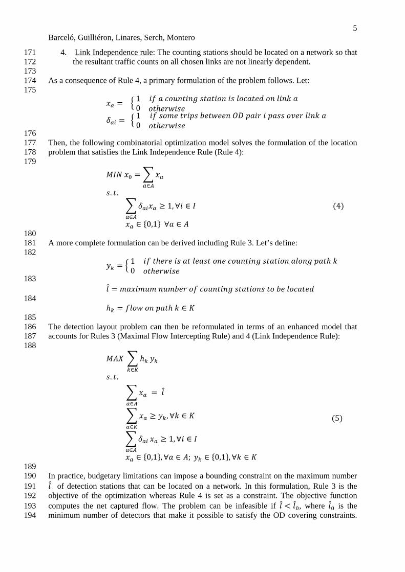
4. Link Independence rule: The counting stations should be located on a network so that 171 the resultant traffic counts on all chosen links are not linearly dependent. 172

173 As a consequence of Rule 4, a primary formulation of the problem follows. Let: 174 175

𝑥𝑎 = � 10𝑖𝑓 𝑎 𝑐𝑜𝑢𝑛𝑡𝑖𝑛𝑔 𝑠𝑡𝑎𝑡𝑖𝑜𝑛 𝑖𝑠 𝑙𝑜𝑐𝑎𝑡𝑒𝑑 𝑜𝑛 𝑙𝑖𝑛𝑘 𝑎𝑜𝑡ℎ𝑒𝑟𝑤𝑖𝑠𝑒

�

𝛿𝑎𝑖 = � 10𝑖𝑓 𝑠𝑜𝑚𝑒 𝑡𝑟𝑖𝑝𝑠 𝑏𝑒𝑡𝑤𝑒𝑒𝑛 𝑂𝐷 𝑝𝑎𝑖𝑟 𝑖 𝑝𝑎𝑠𝑠 𝑜𝑣𝑒𝑟 𝑙𝑖𝑛𝑘 𝑎𝑜𝑡ℎ𝑒𝑟𝑤𝑖𝑠𝑒

� 176 Then, the following combinatorial optimization model solves the formulation of the location 177 problem that satisfies the Link Independence Rule (Rule 4): 178 179

𝑀𝐼𝑁 𝑥0 = �𝑥𝑎𝑎∈𝐴

𝑠. 𝑡. �𝛿𝑎𝑖𝑥𝑎𝑎∈𝐴

≥ 1,∀𝑖 ∈ 𝐼 (4)

𝑥𝑎 ∈ {0,1} ∀𝑎 ∈ 𝐴 180 A more complete formulation can be derived including Rule 3. Let’s define: 181 182

𝑦𝑘 = � 10𝑖𝑓 𝑡ℎ𝑒𝑟𝑒 𝑖𝑠 𝑎𝑡 𝑙𝑒𝑎𝑠𝑡 𝑜𝑛𝑒 𝑐𝑜𝑢𝑛𝑡𝑖𝑛𝑔 𝑠𝑡𝑎𝑡𝑖𝑜𝑛 𝑎𝑙𝑜𝑛𝑔 𝑝𝑎𝑡ℎ 𝑘𝑜𝑡ℎ𝑒𝑟𝑤𝑖𝑠𝑒

� 183

𝑙 = 𝑚𝑎𝑥𝑖𝑚𝑢𝑚 𝑛𝑢𝑚𝑏𝑒𝑟 𝑜𝑓 𝑐𝑜𝑢𝑛𝑡𝑖𝑛𝑔 𝑠𝑡𝑎𝑡𝑖𝑜𝑛𝑠 𝑡𝑜 𝑏𝑒 𝑙𝑜𝑐𝑎𝑡𝑒𝑑 184

ℎ𝑘 = 𝑓𝑙𝑜𝑤 𝑜𝑛 𝑝𝑎𝑡ℎ 𝑘 ∈ 𝐾 185 The detection layout problem can then be reformulated in terms of an enhanced model that 186 accounts for Rules 3 (Maximal Flow Intercepting Rule) and 4 (Link Independence Rule): 187

188 𝑀𝐴𝑋 �ℎ𝑘

𝑘∈𝐾

𝑦𝑘

𝑠. 𝑡. �𝑥𝑎 𝑎∈𝐴

= 𝑙

�𝑥𝑎𝑎∈𝐾

≥ 𝑦𝑘,∀𝑘 ∈ 𝐾

�𝛿𝑎𝑖𝑎∈𝐴

𝑥𝑎 ≥ 1,∀𝑖 ∈ 𝐼

(5)

𝑥𝑎 ∈ {0,1},∀𝑎 ∈ 𝐴; 𝑦𝑘 ∈ {0,1},∀𝑘 ∈ 𝐾 189 In practice, budgetary limitations can impose a bounding constraint on the maximum number 190 𝑙 of detection stations that can be located on a network. In this formulation, Rule 3 is the 191 objective of the optimization whereas Rule 4 is set as a constraint. The objective function 192 computes the net captured flow. The problem can be infeasible if 𝑙 < 𝑙0, where 𝑙0 is the 193 minimum number of detectors that make it possible to satisfy the OD covering constraints. 194


Variants of these formulations can be found in Yang’s paper [12]. An analysis of the 195 advantages and disadvantages of these formulations in terms of the quality of the adjusted OD 196 matrix can be found in the paper by Larsson et al. [13]. 197 198 A common drawback of these formulations is that they require a complete enumeration of all 199 paths between all OD pairs in the road network, which leads to a problem in which the size 200 grows exponentially with the size of the network. A more efficient formulation could be 201 obtained by relaxing the requirement of explicitly enumerating the set of paths and using 202 instead the subset of the most likely used paths. Relaxed formulations of the problem have 203 recently received the attention of researchers (Ehlert et al. [14] and Xiang Fei et al. [15]). 204 205 A MODIFIED FORMULATION OF THE LINK DETECTION LAYOUT PROBLEM 206 ACCOUNTING FOR TIME DEPENDENCIES 207 208 On the basis of the previous discussion, we restrict the path set to the most likely used paths 209 in order to reduce the size of the problem and achieve a higher computational efficiency while 210 not significantly degrading the quality of the solution. Given that the objective of the 211 optimization model is maximum flow interception, and that the most likely used paths are the 212 ones expected to accommodate the greatest number of trips, these paths should be covered 213 even if other paths are used by a minority of travelers 214 215 The approach taken in this paper can be considered as an extension of a previous exploration 216 of the detection layout problem made by Hoogland [16], who explored two alternative 217 formulations: one based on a proposal by Bianco et al. [17] which is rooted in the topological 218 analysis of the network, and another one in which the identification of the most likely used 219 paths for reducing problem size was based on a static equilibrium assignment performed by 220 the Emme commercial package. In the solution produced from the latter, the paths were 221 identified according to a post-processing procedure based on Larsson et al. [18]. A drawback 222 of this approach was that --being based on a static equilibrium assignment-- it did not account 223 for the time dependencies of the used paths. This motivated our research to try and capture 224 this time-dependent nature by identifying the most likely used paths on the basis of a 225 heuristic, dynamic user equilibrium traffic assignment with Dynameq [17]. Fei et al. [20] also 226 exploit the advantages of formulating the problem in terms of the most likely used paths as 227 determined by the dynamic user equilibrium achieved by DYNASMART, but their 228 formulation is based on the simplified model discussed in (4). An additional feature of a 229 formulation based on a dynamic traffic assignment is that, due to explicitly accounting for 230 time dependencies, the identified paths and the corresponding link proportions can be time 231 sliced, leading to the following enriched time-dependent formulation of the detection layout 232 problem: 233 234 235

236 237 238 (6) 239 240 241 242 243 244

{ } { } Kk,0,1y A,a,0,1x

TτI,i 1,xδ

Kk ,yx

lx

yh MAX

ka

Aaa

τai

kka

a

Aaa

Tτ Kkk

τk

∈∀∈∈∀∈

∈∀∈∀≥

∈∀≥

=

∑

∑

∑

∑∑

∈

∈

∈

∈ ∈

ˆ


Where ℎ𝑘τ is the flow on path k at time interval τ, τδ ai indicates if link a is part of one of the 245 most likely paths between OD pair i at time intervalτ. With this restriction, we have a 246 maximum number of paths that is equal to NIx|T|xM, where M is the maximum number of 247 paths that are considered for each OD pair for each time interval (usually 3 or 4) and |T| is the 248 number of time intervals. This number can be great, but does not grow exponentially with the 249 number of links in the network, and therefore is acceptable even for large networks. The 250 resulting set covering problem with side constraints has a richer and improved structure 251 compared to the previous one studied in [16]. From a computational point of view, the main 252 difference lies in the fact that the resulting formulation can be efficiently pre-processed to 253 reduce its size by using the pre-processing techniques that are proper for combinatorial 254 optimization (Savelsbergh [20]). This allows the identification of dominated columns and 255 rows, clique inequalities and other pertinent characteristics in the combinatorial structure of 256 the set of constraints (6). The equivalent pre-processed problem is then solved by an ad hoc 257 combination of tabu search and diversification heuristics (Hertz et al. [21]) in a modified 258 problem formulation, which subsequently relaxes the OD covering rule in a Lagrangian 259 fashion. 260 261 The tabu search is a local search method developed by Glover [22]. This algorithm tries to 262 improve the current solution by choosing the best in the neighborhod, but it avoids some 263 specific movements in order to increase the chances of leaving a local optimum. The 264 algorithm keeps a list of forbidden movements --called a tabu list-- at each iteration; the next 265 solution is then given by the best neighbor solution that does not need to reach a tabu 266 movement. When the movement iscompleted, the inverse movement is added to the tabu list 267 and will stay inside it for a fixed number of iterations. This will force the algorithm to search 268 further, even if it is necessary to go through worse solutions. To avoid being too restrictive, a 269 tabu movement will nevertheless be authorized if it reaches a solution that is better than any 270 other found in the entire algorithm. 271 272 An algorithm capable of finding a good solution for any number of detectors is desirable, but 273 it is not possible to know if this number is great enough to satisfy the OD covering rule or not. 274 Even if it is possible to find a feasible solution, it could be less desirable to satisfy the OD 275 covering rule while intercepting a small fraction of the total flow instead of not covering a 276 few OD pairs while intercepting almost all the flow in the network. Following these 277 considerations, the choice was made to no longer consider the OD covering rule as a 278 constraint, but to introduce it instead into the objective function, which permits not only 279 dealing with the fact that these constraints may not be feasible, but it also gives a direct means 280 for evaluating the quality of a solution. Indeed, it is necessary to evaluate whether a solution 281 that covers more OD pairs but less flow is better or worse than another solution. This has to 282 be done by weighting what is more important: to satisfy Rule 1 (OD covering rule) by 283 weighting the coefficient ρ2, or to follow Rule 3 (maximal flow intercepting rule) by 284 weighting coefficient ρ1. The problem was therefore reformulated as follows: 285 286

{ } { } Kk,0,1yA,a,0,1x

Kk,yx

lx s.t.

sConstraint OD #Satisfieds Constraint OD#ρ

FlowTotal Flowd Intercepteρ MAX

ka

kka

a

Aaa

21

∈∀∈∈∀∈

∈∀≥

=

+

∑

∑

∈

∈

ˆ (7) 287


288 Where the intercepted flow is given by ∑∑

∈ ∈Tτ Kkk

τk yh 289

The OD covering rule constraint ∑ 𝛿𝑎𝑖𝜏 𝑥𝑎 ≥ 1,∀𝑖 ∈ 𝐼,∀𝜏𝜖𝑇𝑎∈𝐴 is replaced by another one, 290 using the path variables instead of the link variables: 291

�𝛿𝑘𝑖𝜏 𝑦𝑘 ≥ 1,∀𝑖 ∈ 𝐼,∀𝜏 ∈ 𝑇𝑘∈𝐾

Where 𝛿𝑘𝑖𝜏 �= 1 𝑖𝑓 𝑝𝑎𝑡ℎ 𝑘 𝑐𝑜𝑛𝑛𝑒𝑐𝑡𝑠 𝑡ℎ𝑒 𝑖 − 𝑡ℎ 𝑂𝐷 𝑝𝑎𝑖𝑟= 0 𝑂𝑡ℎ𝑒𝑟𝑤𝑖𝑠𝑒

� . This constraint still represents the 292 OD covering rule, but now the left side member contains only a few variables, as the 293 maximum number of paths for each OD pair is fixed. 294 295 Greedy algorithm for initialisation 296 297 The initial solution is found by the following greedy algorithm: 298 299

1. Initialisation 300 Compute total flows on each link. 301 2. While some detectors aren't placed and some links have non-zero flow, do 302 (a) Find link with greatest flow, add a detector to it. 303 (b) For each path going through this link: 304 set flow to zero. 305 change link flows according to it. 306 3. Return to detector’s location 307

308 This greedy algorithm gives a solution that covers a great fraction of total flow, and therefore 309 is a good start for the tabu search; but it is not optimal, neither for the number of OD 310 constraints nor the flow. 311 312 Next movement's choice 313 314 A movement from one solution to another is defined as the move of a detector to a new 315 location, which is on the one hand relatively simple to try and find, and on the other hand 316 allows us to reach every possible solution. As a criterion for measuring a movement's quality, 317 the improvement of the objective function (7) is considered. In order to find the best 318 movement, detectors must be treated one by one, first by removing it and then by trying to 319 insert a new detector located at each empty link. 320 321

1. Given: 322 Set of links containing detectors 323 Updated data for current solution with flows and constraints 324 Evaluation function 325 2. For each detector in the set, do: 326 (a) Remove detector and update data 327 (b) If new flow on link where the detector was located is 0: 328 Choose best available link to put detector. 329 STOP (the detector was useless). 330

(c) Else 331 For each link without detector 332

Evaluate movement with evaluation function. 333


Keep if best. 334 3. Do best movement and update data. 335

336 Tabu List Update 337 338

1. Given: 339 TabuList containing elements of the type (start; end; iteration), where 340 start is the link where the detector was, end is the link where detector is 341 placed, iteration is a step counter 342 TabuListSize which represent the oldest movement that is considered in 343 tabu list 344 New movement m = (start; end; iteration) 345 2. Add inverse movement (end; start; iteration) to TabuList 346 3. For each movement m’ in TabuList, do 347 (a) If m’.iteration = m.iteration _ TabuListSize 348 Remove m’ from TabuList 349 (b) Else if m’.start = m.end 350 Add movement (m.start;m’.end;m’.iteration) to TabuList 351 4. Return TabuList 352

353 With this definition of movement, two neighbor solutions are very close. In order to explore a 354 large part of the solution space, we have to add a diversification phase to our algorithm, 355 because the tabu list can't be big enough to ensure diversification, as it has to remain 356 reasonable in order to intensively explore the neighborhood. When the current solution isn’t 357 improved during the last iterations of k, we temporally change the objective function to 358 𝑀𝐼𝑁 ∑ 𝑛(𝑎)𝑥𝑎𝑎∈𝐴 , where n(a) is a frequency counter for placing a detector on link a, in 359 order to reach an unexplored area. The tabu search then starts again. 360 361 COMPUTATIONAL RESULTS FOR THE LINK LAYOUT MODEL 362 363 A set of computational experiments has been conducted with various networks. Due to the 364 limitation of space, we illustrate the results by presenting here only those which correspond to 365 the Eixample district in Barcelona, with the infrastructure corresponding to May 2005. This 366 network, depicted in Figure 1, has 1570 sections, 692 intersections and 210 centroids. The 367 Origin-Destination matrix we started with corresponds to the traffic between 8 am and 9 am. 368 The OD matrix for this network was also split into four different matrices corresponding to 369 four different time slices, using the following percentages: 15%, 30%, 40% and 15%. There 370 were initially 1570 links that were reduced to 1289 by preprocessing; 531 clique inequalities 371 were found. The equilibrium gave 8242 paths, reduced to 3107, for 1358 OD pairs during 4 372 time periods, which means a total number of 4944 initial OD constraints. This number falls 373 down to 2609 when not considering the repeated constraints, and to 2045 when suppressing 374 the redundant ones. The total flow assigned to the Barcelona network was 63973 trips, and the 375 minimum number of detectors to cover the 1236 OD pairs is 115. Table 1 summarizes the 376 numerical results and the red stars in Figure 1 identify the proposed detector locations. Our 377 heuristic intercepts a large fraction of total flow (63973 vehicles), but also covers almost each 378 OD pair in the network, which is important for limiting the OD matrix estimation error. 379 380


381 Figure 1 - Detection layout for Barcelona’s model 382

383 Detectors Theoretical solution :

intercepted flow Constraints satisfied Heuristic solution :

flow intercepted Constraints satisfied

100 63890 (99.9%) 1975/2045 ~63490 (99.2%) ~2022/2045 115 63390 (99.1%) 2045/2045 ~63780 (99.7%) ~2039/2045 120 63943 (~100%) 2045/2045 ~63850 (99.8%) ~2043/2045 130 63973 (100%) 2045/2045 ~63970 (~100%) 2045/2045

Table 1 - Computational results for Barcelona’s network 384 385 Table 2 reports on the quality of the computational results with a comparison of the problem’s 386 exact solutions that were obtained by CPLEX. The heuristic was modified to account for 387 additional practical considerations, like limiting a priori the number of detectors to locate, a 388 constraint that could be imposed in practice by budgetary conditions. Another practical 389 limitation would be bounding the percentage of the total number of trips intercepted by the 390 detectors, a constraint that could be imposed in certain conditions as a measure of the quality 391 of the solution. Two other networks were used: 392 393

• The network of the City of Preston, in Lancashire UK, containing 417 links, 166 394 nodes (intersections) and 34 centroids representing origins and/or destinations. 395

• And the highway network of the Hessen land in Germany, with 4282 links (road 396 sections), 495 nodes (intersections) and 245 centroids (origins/destinations). 397

398


399 Table 2 - Comparative results of the exact and heuristics solutions with additional 400

constraints 401 Table 2 compares the exact solution with CPLEX, the greedy heuristic and the tabu heuristic 402 in terms of the number of detectors, the % of the total flow intercepted and the % of OD 403 constraints satisfied in model (7). 404 405

406 Figure 2 - Covered flow and OD constraints in Preston network 407

408 Figure 2 graphically illustrates the quality of the solution in terms of % of intercepted flows 409 and % of satisfied OD constraints as a function of the number of detectors. It can be observed 410 that both the flow and the constraints covered are improved very quickly with a small number 411 of detectors. They then need a large number of additional counts to reach a total cover. The 412 same phenomenon is observable in the Barcelona and Hessen networks. 413 414 THE INTERSECTION DETECTION LAYOUT PROBLEM 415 416 Most of the new applications based on Information and Communications Technology (ICT) 417 work in a different way from the traditional ones; they are able to capture the electronic or 418


magnetic signature of specific on-board devices. One of the most typical of such sensors is 419 that which is capable of capturing a Bluetooth equipped device on board a vehicle. The basic 420 principles on how these sensors operate are the following: A vehicle equipped with a 421 Bluetooth device traveling along the freeway is logged and time-stamped at time t1 by the 422 sensor at location 1. After traveling a certain distance it is logged and time-stamped again at 423 time t2 by the sensor at location 2 downstream. The difference in time stamps τ = t2 – t1 424 measures the travel time of the vehicle equipped with that mobile device. Obviously the speed 425 is also measured, assuming that the distance between both locations is known. Data captured 426 by each sensor is sent for processing to a central server by wireless telecommunications. 427 428 However, when dealing with sensors that capture the electronic signature as described, and 429 specifically when these are detectors of Bluetooth devices on board vehicles, the observability 430 problem in terms of detector location must be formulated in different terms by taking into 431 account that these detectors are more efficiently located at intersections and not at links, 432 where they can capture a higher number of vehicles. Let’s analyze the scheme in Figure 3, 433 assuming that the Bluetooth sensor is located at the intersection in a location in such a way 434 that its detection lobule intercepts all equipped vehicles crossing the node on paths (1), (2), 435 (3) and (4). The candidate intersections would be those intercepting a higher number of 436 equipped vehicles. 437 438 439 440 441 442 443 444 445 446

Figure 3 - Flows intercepted from paths crossing a node 447 Following the same four modeling hypotheses proposed in the formulation of the link 448 detection layout problem, and as a consequence of Rule 3 (Maximal Flow Intercepting Rule), 449 a primary formulation of the intersection layout problem is the following. Let: 450 451

𝑥𝑛 = � 10𝑖𝑓 𝑎 𝑠𝑒𝑛𝑠𝑜𝑟 𝑖𝑠 𝑙𝑜𝑐𝑎𝑡𝑒𝑑 𝑎𝑡 𝑖𝑛𝑡𝑒𝑟𝑠𝑒𝑐𝑡𝑖𝑜𝑛 𝑛𝑜𝑡ℎ𝑒𝑟𝑤𝑖𝑠𝑒

�

𝑦𝑘 = � 10𝑖𝑓 𝑡ℎ𝑒𝑟𝑒 𝑖𝑠 𝑎𝑡 𝑙𝑒𝑎𝑠𝑡 𝑜𝑛𝑒 𝑑𝑒𝑡𝑒𝑐𝑡𝑜𝑟 𝑎𝑙𝑜𝑛𝑔 𝑝𝑎𝑡ℎ 𝑘𝑜𝑡ℎ𝑒𝑟𝑤𝑖𝑠𝑒

�

𝛿𝑛𝑘 = � 10𝑖𝑓 𝑖𝑛𝑡𝑒𝑟𝑠𝑒𝑐𝑡𝑖𝑜𝑛 𝑛 𝑖𝑠 𝑖𝑛𝑡𝑜 𝑝𝑎𝑡ℎ 𝑘𝑜𝑡ℎ𝑒𝑟𝑤𝑖𝑠𝑒

� 452

𝑙 = 𝑚𝑎𝑥𝑖𝑚𝑢𝑚 𝑛𝑢𝑚𝑏𝑒𝑟 𝑜𝑓 𝑑𝑒𝑡𝑒𝑐𝑡𝑜𝑟𝑠 𝑡𝑜 𝑏𝑒 𝑙𝑜𝑐𝑎𝑡𝑒𝑑 𝐾 = 𝑠𝑒𝑡 𝑜𝑓 𝑎𝑙𝑙 𝑝𝑎𝑡ℎ𝑠 𝑏𝑒𝑡𝑤𝑒𝑒𝑛 𝑎𝑙𝑙 𝑂𝐷 𝑝𝑎𝑖𝑟𝑠 𝐾𝑖 = 𝑠𝑒𝑡 𝑜𝑓 𝑝𝑎𝑡ℎ𝑠 𝑓𝑜𝑟 𝑡ℎ𝑒 𝑖𝑡ℎ 𝑂𝐷 𝑝𝑎𝑖𝑟;𝐾 = � 𝐾𝑖

𝑖∈𝐼

ℎ𝑘 = 𝑓𝑙𝑜𝑤 𝑜𝑛 𝑝𝑎𝑡ℎ 𝑘 ∈ 𝐾 453 𝑁 = 𝑠𝑒𝑡 𝑜𝑓 𝑖𝑛𝑡𝑒𝑟𝑠𝑒𝑐𝑡𝑖𝑜𝑛𝑠 (𝑛𝑜𝑑𝑒𝑠)𝑜𝑓 𝑡ℎ𝑒 𝑛𝑒𝑡𝑤𝑜𝑟𝑘𝐼 = 𝑠𝑒𝑡 𝑜𝑓 𝑎𝑙𝑙 𝑂𝐷 𝑝𝑎𝑖𝑟𝑠 𝑖𝑛 𝑡ℎ𝑒 𝑛𝑒𝑡𝑤𝑜𝑟𝑘

If path k carries flow ℎ𝑘 , then ∑ ℎ𝑘𝑘∈𝐾𝑛 is the total flow captured by the detector at node n. 454 Kn is the set of paths crossing node n. Based on the experience with the previous link 455

(1

(2

(3 (4


covering models, the problem is formulated in terms of the most likely used paths determined 456 by the solution of a Dynamic User Equilibrium Assignment with Dynameq [19]. We would 457 be interested in identifying which is the configuration of nodes that maximizes the total flow 458 intercepted by the sensors located there; therefore, we formulate the objective function in 459 terms of Rule 3 by representing the total intercepted flow. To enhance the OD covering, we 460 impose the condition that at least one path of each OD pair has a detector located on it, and 461 for practical reasons we also include a bounding constraint on the maximum number 𝑙 of 462 detectors that can be located in a network. The problem can then be formulated in terms of the 463 following extended set covering model with side constraints: 464 465

𝑴𝑨𝑿 �𝒉𝒌 ∙ 𝒚𝒌 𝒌∈𝑲

𝑠. 𝑡.

� 𝑥𝑛𝑛 ∈𝑁

≤ 𝑙

�𝛿𝑛𝑘 ∙ 𝑥𝑛 ≥ 𝑦𝑘 ,𝑛∈𝑁

∀𝑘 ∈ 𝐾𝑖 ,∀𝑖 ∈ 𝐼

� 𝑦𝑘 ≥ 1𝑘∈𝐾𝑖

, ∀𝑖 ∈ 𝐼

𝑥𝑛,𝑦𝑘 ∈ {0,1}

(8)

In this formulation the problem can be infeasible if 𝑙 < 𝑙0, where 𝑙0 is the minimum number 466 of detectors necessary to satisfy the OD covering constraints. Therefore we quantify the 467 infeasibility when it appears. To this end, the proposed third intersection detection layout 468 formulation is the previously presented formulation, adding the OD covering rule in a 469 Lagrangian fashion. Let: 470 471

𝑧𝑖 = � 1 𝑖𝑓 𝑖𝑡ℎ 𝑂𝐷𝑝𝑎𝑖𝑟 𝑖𝑠 𝑐𝑜𝑣𝑒𝑟𝑒𝑑 𝑎𝑡 𝑙𝑒𝑎𝑠𝑡 𝑏𝑦 𝑜𝑛𝑒 𝑑𝑒𝑡𝑒𝑐𝑡𝑜𝑟 0 𝑜𝑡ℎ𝑒𝑟𝑤𝑖𝑠𝑒

�

472

𝑀𝐴𝑋 𝐹(𝑦, 𝑧) = 𝛼 ∙∑ ℎ𝑘 ∙ 𝑦𝑘 𝑘∈𝐾∑ ℎ𝑘 𝑘∈𝐾

+ 𝛽 ∙∑ 𝑧𝑖 𝑖∈𝐼

|𝑂𝐷|

473 𝑠. 𝑡.


≤ 𝑙 ̂

�𝛿𝑛𝑘 ∙ 𝑥𝑛 ≥ 𝑦𝑘 ,𝑛∈𝑁

∀𝑘 ∈ 𝐾𝑖 ,∀𝑖 ∈ 𝐼

� 𝑦𝑘 ≥ 𝑧𝑖𝑘∈𝐾𝑖

, ∀𝑖 ∈ 𝐼

𝑥𝑛,𝑦𝑘 ∈ {0,1}

(9)

The sensitivity analysis of the Lagrangian multipliers 𝛼,𝛽 allows us to identify which is the 474 total flow intercepted by the detectors that can be interpreted either in terms of an error bound 475


or the quality of the traffic information that can be generated. The analysis of the infeasibility 476 also reveals which are the uncovered OD pairs. A proper selection of 𝑙 provides a solution 477 that captures 100% of the traffic demand, ensuring in this way the complete observability of 478 the system. 479 480 The location of Bluetooth sensors can raise an additional question in terms of the 481 measurement of travel times between pairs of detectors along the likely used paths, as has 482 been described in the introduction of this section. In order to achieve this objective, we 483 propose a new formulation of the model that adds two sets of constraints: 484 485

• Ensuring a minimum number of detectors on each path, and 486 • Imposing a condition of minimum linear distance between two detectors. This 487

constraint can also be justified from the technological point of view of minimizing the 488 likelihood of improper detection due to signal overlapping. 489

490 The new formulation would then be: 491 492

𝑀𝐴𝑋 �ℎ𝑘 ∙ 𝑦𝑘

𝑘∈𝐾

𝑠. 𝑡.


≤ 𝑙

�𝛿𝑛𝑘 ∙ 𝑥𝑛 ≥ 𝑝𝑦𝑘 ,𝑛∈𝑁

∀𝑘 ∈ 𝐾𝑖 ,∀𝑖 ∈ 𝐼 (∗)

� 𝑦𝑘 ≥ 1𝑘∈𝐾𝑖

, ∀𝑖 ∈ 𝐼 (10)

𝑥𝑖 + 𝑥𝑗 ≤ 1 ∀𝑖,∀𝑗 ∈ 𝑉(𝑖)

𝑥𝑛,𝑦𝑘 ∈ {0,1}

Where: 493 • 𝑉(𝑖) is the linear neighborhood of intersection i, defined as: 494

𝑉(𝑖) = {𝑗 ∈ 𝐼|𝑑𝑖𝑠𝑡(𝑖, 𝑗) ≤ 𝑚 𝑚𝑒𝑡𝑒𝑟𝑠} • p is the parameter defining the minimum number of detectors per path, constraints (*) 495

provide path information; p > 1 provides travel times between detectors along a path 496 • m is the minimum linear distance between two detectors 497

498 COMPUTATIONAL RESULTS FOR THE INTERSECTION LAYOUT MODEL 499 500 A set of computational experiments has been conducted in the same scenario proposed for the 501 link covering problem: the Eixample district in Barcelona. An updated OD matrix 502


corresponding to the traffic between 8 am and 9 am for a typical weekday of 2007 is utilized. 503 The exact solutions for the different proposed experiments have been obtained with CPLEX. 504 Due to space constraints we will report here only the computational results for models (9) and 505 (10). Figure 4 depicts the sensitivity analysis of the Lagrangian multipliers in a restrictive 506 case when the number of available detectors is fixed at 10 in model (9). 507

508

509 Figure 4 - Lagrangian multipliers sensitivity analysis 510

Table 3 summarizes the reverse experiment, fixing the Lagrangian multipliers (𝛼,𝛽) to 0.5, in 511 order to simulate a situation where the relative importance of capturing flow and covering OD 512 pairs is the same. Then, the model is executed with 𝑙 = 1 until 𝑙 = 80, increasing the value 513 one by one. 514

Used Detectors (D) Captured Flow Covered OD Pairs O.F. 1 12,65 17,66 15,16 2 21,97 31,58 26,77 3 30,53 43,74 37,14 4 40,29 48,89 44,59 5 45,38 56,02 50,70 6 50,13 61,29 55,71 7 56,23 65,15 60,69 8 62,04 69,12 65,58 9 66,87 71,58 69,22 10 71,50 74,15 72,83 … … … … 15 84,52 85,26 84,89 … … … … 20 91,90 92,28 92,09 … … … … 25 95,59 96,49 96,04 … … … … 30 98,26 98,83 98,55 … … … … 40 99,83 100,00 99,91 … … … … 80 99,98 100,00 99,99

515 Table 3 – Summary of captured flow and covered OD pairs for 𝜶 = 𝜷 = 𝟎.𝟓 516

517


Figure 5 displays the graphics of the percentage of intercepted OD flows as a function of the 518 number of detectors located by model (10). 519

520

521 522 523

RESULTS FLOW Total flow 50136,58 Intercepted flow on paths with detectors 45379,48 % of total flow intercepted 90,51% OD PAIRS Total number of OD pairs 881 Number of covered OD pairs 753 Proportion of covered OD pairs 85,47% PATHS Total number of paths 1977 Total number of covered paths 1692 Proportion of covered paths 85,58%

524

Table 4 Summary of numerical results for model (10) for �̂� = 𝟓𝟎 Bluetooth sensors 525

Table 4 summarizes the analysis of the quality of the solution in terms of the total amount of 526 intercepted OD flows and OD pairs for 𝑙 = 50, p = 2 and m=300 meters. 527

Figure 5. Percentage of intercepted flow as a function of the number of detectors


528

Figure 6 Optimal location of 50 Bluetooth detectors by model (10) with p=2 and m=300 529

Figure 6 displays the location of the 50 detectors and an example of some sections of the main 530 paths whose travel times are estimated by Bluetooth detection. 531

532 CONCLUSIONS 533 534 By considering only the most probable paths, the new approach proposed for the link 535 detection layout problem reduces the size of the problem considerably when including time 536 periods. Consequently, it ensures that a good estimation is possible. This formulation 537 appeared to be very sensitive to pre-processing, which can further reduce the size of the 538 problem. When solved with CPLEX, it appears to be well conditioned as almost no more pre-539 processing is found by the software, and the resolution time is very short. Even with time 540 considerations, the number of detectors necessary to satisfy the OD covering rule stays 541 reasonable, unlike other previous formulations with time periods. This shows that the new 542 theoretical model is very good and realistic for practical use. 543 544 The reformulation of the problem in terms of intersection detection layout shows an even 545 better performance in substantially reducing the number of detectors needed to maximize the 546 total intercepted flow and/or the number of OD constraints. 547 548 ACKNOWLEDGEMENTS 549 550 The research reported in this project has been funded by projects MITRA (TRA2009-14270 551 (subprogram MODAL, FEDER Co funded)) and In4Mo (TSI-020100-2010-690) of the Spanish 552 R+D National Programs 553 554 555 REFERENCES 556 557 [1] Florian M. and Hearn D. (1995), Network Equilibrium Models and Algorithms, 558

Chapter 6 in: M.O. Ball et al., Eds., Handbooks in OR and MS, Vol.8, Elsevier Science 559 B.V. 560

[2] Ben-Akiva, M., Bierlaire, M., Burton, D., Koutsopoulos, H.N. and Mishalani, R., 561 (2001), Network State Estimation and Prediction for Real-Time Traffic Management, 562 Networks and Spatial Economics, 1, pp. 293-318. 563

[3] Cascetta, E. (2001) Transportation Systems Engineering: Theory and Methods, 564 Chapter 8, Kluwer Academic Publishers. 565


[4] Van Zuylen, H.J. and Willumsen, L.G. (1980) The most likely trip matrix estimated from 566 traffic counts, Transportation research Part B, 14, pp. 281-293. 567

[5] Codina E., Barceló,J. (2004) Adjustment of O-D matrices from observed volumes: an 568 algorithmic approach based on conjugate gradients, European Journal of Operations 569 Research, Vol. 155, pp. 535-557. 570

[6] Lundgren J. T. and Peterson A. (2008), A heuristic for the bilevel origin–destination-571 matrix estimation problem, Transportation Research Part B 42 (2008) 339–354 572

[7] Ashok, K. and Ben-Akiva, M., (2000) Alternative Approaches for Real-Time 573 Estimation and Prediction of Time-Dependent Origin-Destination Flows, Transportation 574 Science 34(1), 21-36. 575

[8] Antoniou, C., Ben-Akiva, M. and Koutsopoulos H.N., (2007), Nonlinear Kalman 576 Filtering Algorithms for On-Line Calibration of Dynamic Traffic Assignment Models, 577 IEEE Transactions on Intelligent Transportation Systems Vol. 8 No.4. 578

[9] Barceló J., Montero L., Marqués L. and Carmona C., (2010), Travel time forecasting 579 and dynamic of estimation in freeways based on Bluetooth traffic monitoring, 580 Transportation Research Records: Journal of the Transportation Research Board, Vol. 581 2175, pp. 19-27. 582

[10] Bierlaire, M., (2002), The Total Demand Scale: a New Measure of Quality for Static 583 andDynamic Origin-Destination Trip Tables, Transpn. Res. B 36, 837-850. 584

[11] Castillo, E. Conejo, A. J. Menéndez, J. M. Jiménez, P., (2008, The Observability 585 Problem in Traffic Network Models, Computer-Aided Civil and Infrastructure Engineering 586 23, 208–222 587

[12] Yang, H., and Zhou, J. (1998), “Optimal Traffic Counting Locations for Origin-588 Destination Matrix Estimation”, Transp. Res. B, Vol. 32B, No.2, pp.109-126 589

[13] Larsson, T. Lundgren, J.T. and Peterson, A. (2010), Allocation of Link Flow 590 Detectors for Origin-Destination Matrix estimation a Comparative Study, Computer-Aided 591 Civil and Infrastructure Engineering, 25, pp. 116-131. 592

[14] Ehlert, A.,. Bell, M. G.H and Grosso, S. (2006), The Optimisation of Traffic Count 593 Locations in Road Networks, Transportation research Part B 40, pp. 460-479. 594

[15] Fei, X., Eisenman, S. M. and Mahmassani, H.,(2007) Sensor Coverage and Location 595 for Real-Time Traffic Prediction in Large-Scale Networks, Paper presentes at the 86th 596 Annual Meeting of the Transportation Research Board, January 2007. 597

[16] Hoogland, J.K. (2000), The traffic sensor location problem, Master Thesis, Delft 598 University 599

[17] Bianco, L. Confessore, G. and Reverberi, P. (2001), A Network Based Model for 600 Traffic Sensor Location with Implications on O-D Matrix Estimates, Transportation 601 Science 35, pp. 50-60. 602

[18] Larsson, T., Lundgren, J.T., Patriksson, M. and Rydergreen, C. (1998), Most likely 603 equilibrium route flows: analysis and computation, Proceedings of TRISTAN III. 604

[19] Dynameq 1.4, (2010), INRO Consultants, Montreal 605 [20] Savelsbergh, M.W.P. (1994), Preprocessing and Probing Techniques for Mixed 606

Integer Programming Problems. ORSA J. Comput. 6, 445-455. 607 [21] Hertz, A., Taillard, E.D., de Werra, D., (1997) A Tutorial on Tabu Search. Local 608

Search in Combinatorial Optimization, E. Aarts and J.K. Lenstra (Eds), 121-136. 609 [22] Glover, F. (1986) Future Paths for Integer Programming and Links to Artificial 610

Intelligence. Computers and Operations Research 13, 533-549. 611

exploring link covering and node covering formulations of

Documents