Exploring Image and Video by Classification and Clustering on

Global and Local Visual Features

By

Le Lu

M.S.E. Johns Hopkins University 2004

B.E. Beijing Polytechnic University 1996

A Dissertation submitted to

The Faculty of

Whiting School of Engineering

of The Johns Hopkins University in partial satisfaction

of the requirements for the degree of Doctor of Philosophy

Fall 2006

Dissertation directed by

Gregory D. Hager

Professor of Computer Science

i

Abstract of Dissertation

Images and Videos are complex 2-dimensional spatial correlated data pattern or 3-dimensional spatial-

temporal correlated data volumes. Associating these correlated relationships of visual data signals (acquired

by imaging sensors) with high-level semantic human knowledge is the core challenging problem of pat-

tern recognition and computer vision. Finding the inter-correlated relationships across multiple different

images or videos, given a large amount of data in similar or non-similar scenarios, without direct anno-

tation from human concepts, is another self-organized data structuring issue. From the previous literature

and our own research work [9, 11, 12, 13, 14, 15], via computing machines as tools, there are a lot of

efforts trying to address these two tasks statistically, by making good use of recently developed super-

vised (a.k.a. Classification) and Unsupervised (a.k.a. Clustering) statistical machine learning paradigms

[1, 5, 26, 7, 165, 19, 145, 2, 18].

In this dissertation, we are particularly interested to study four specific yet important computer vision

problems involving partitioning, discriminative multiple-class classification and online adaptive appearance

learning, depending on statistical machine learning techniques. Our four tasks are based on extracted global

and local visual appearance patterns from both image and video domains respectively. First, we develop

new unsupervised clustering algorithm to partition temporal video structure (a.k.a. video shot segmen-

tation) [12]. Second, we detect and recognize spatial-temporal video volumes as action unites through

trained 3D surface model and multi-scale temporal searching [60]. The 3D surface based action model is

obtained as output of the learning process of texton-like [121] intermediate visual representations, using

sequentially adapted clustering from figure-segmented image sequences [9]. Third, we train discriminative

multi-modal probabilistic density classifiers to detect semantic material classes from home photo in a soft

ii

classification manner. Learning photo categories is then based the global image features extracted from

the material class-specific density response maps by random weak classifier combination [68, 103, 162] to

handle the complex photo-feature distribution in high dimensions [11]. Fourth, we propose a unified ap-

proach for close-field (medium to high resolution) segmentation based object matching and tracking (a.k.a

video matting [73, 124, 161]), and far-field localization based object tracking [?, 96]. The main novelty

exists on two folds: our framework that allows very flexible image density matching function construction

[5, 165, 69, 100, 106, 11, 87, 86, 71]; our bi-directional appearance consistency check algorithm which has

been demonstrated to maintain an effective object-level appearance models under different severe chang-

ing, occluding and deformable appearance situations and camera imaging conditions, but only require very

simple nonparametric similarity computations [14].

iii

Acknowledgments

Thank some people here.

iv

Contents

Abstract of Dissertation ii

Acknowledgments iv

Introduction xiv

0.1 Motivation . . . . . . . . . . . . . . . . . . . . . . . . . . . . . . . . . . . . . . . . . . . . xiv

1 Partitioning Temporal Video Structure:

A Combined Central and Subspace Clustering Approach 1

1.1 Introduction . . . . . . . . . . . . . . . . . . . . . . . . . . . . . . . . . . . . . . . . . . . 2

1.1.1 Review on Clustering Methods . . . . . . . . . . . . . . . . . . . . . . . . . . . . . 2

1.1.2 Failure or Success: Two Toy Problems? . . . . . . . . . . . . . . . . . . . . . . . . 3

1.1.3 Proposed Clustering Method . . . . . . . . . . . . . . . . . . . . . . . . . . . . . . 5

1.2 Algorithm: Combined Central-Subspace Clustering . . . . . . . . . . . . . . . . . . . . . . 5

1.3 Experiments: Clustering Performance Evaluation . . . . . . . . . . . . . . . . . . . . . . . 10

1.3.1 Comparison: Central clustering and subspace clustering . . . . . . . . . . . . . . . 10

1.3.2 Performance Evaluation on simulated data . . . . . . . . . . . . . . . . . . . . . . . 12

1.4 Experiments: Illumination-invariant face clustering . . . . . . . . . . . . . . . . . . . . . . 13

1.5 Experiments: Video shot segmentation . . . . . . . . . . . . . . . . . . . . . . . . . . . . . 14

1.6 Discussion on Model Selection . . . . . . . . . . . . . . . . . . . . . . . . . . . . . . . . . 16

1.6.1 Practical Solution . . . . . . . . . . . . . . . . . . . . . . . . . . . . . . . . . . . . 17

v

1.7 Conclusions and Future Work . . . . . . . . . . . . . . . . . . . . . . . . . . . . . . . . . . 17

2 Recognizing Temporal Units of Video using Textons:

A Three-tiered Bottom-up Approach of Classifying Articulated Object Actions 26

2.1 Introduction . . . . . . . . . . . . . . . . . . . . . . . . . . . . . . . . . . . . . . . . . . . 27

2.2 A Three Tiered Approach . . . . . . . . . . . . . . . . . . . . . . . . . . . . . . . . . . . . 29

2.2.1 Low Level: Rotation Invariant Feature Extraction . . . . . . . . . . . . . . . . . . . 29

2.2.2 Intermediate Level: Clustering Presentation (Textons) for Image Frames . . . . . . . 30

2.2.3 High Level: Aggregated Histogram Model for Action Recognition . . . . . . . . . . 33

2.3 Results . . . . . . . . . . . . . . . . . . . . . . . . . . . . . . . . . . . . . . . . . . . . . . 36

2.3.1 Convergency of Discriminative-GMM. . . . . . . . . . . . . . . . . . . . . . . . . 36

2.3.2 Framewise clustering. . . . . . . . . . . . . . . . . . . . . . . . . . . . . . . . . . 36

2.3.3 Action recognition and segmentation. . . . . . . . . . . . . . . . . . . . . . . . . . 37

2.3.4 Integrating motion information. . . . . . . . . . . . . . . . . . . . . . . . . . . . . 38

2.4 Conclusion and Discussion . . . . . . . . . . . . . . . . . . . . . . . . . . . . . . . . . . . 39

3 Discriminative Learning of Spatial Image Distribution:

A Two-level Image Spatial Representation for Image Scene Category Recognition 40

3.1 Introduction . . . . . . . . . . . . . . . . . . . . . . . . . . . . . . . . . . . . . . . . . . . 41

3.2 Previous Work . . . . . . . . . . . . . . . . . . . . . . . . . . . . . . . . . . . . . . . . . . 42

3.3 Local Image-Level Processing . . . . . . . . . . . . . . . . . . . . . . . . . . . . . . . . . 43

3.3.1 Color-Texture Descriptor for Image Patches . . . . . . . . . . . . . . . . . . . . . . 45

3.3.2 Discriminative Mixture Density Models for 20 Materials . . . . . . . . . . . . . . . 46

3.4 Global Image Processing . . . . . . . . . . . . . . . . . . . . . . . . . . . . . . . . . . . . 47

3.4.1 Global Image Descriptor . . . . . . . . . . . . . . . . . . . . . . . . . . . . . . . . 47

3.4.2 Week Learner: LDA Classifers with Bootstrapping and Random Subspace Sampling 48

3.5 Experiments . . . . . . . . . . . . . . . . . . . . . . . . . . . . . . . . . . . . . . . . . . . 49

vi

3.5.1 Local Recognition: Validation of Image Patches Representation for Material Classes 49

3.5.2 Global Recognition: Photo based Scene Category Classification . . . . . . . . . . . 50

3.6 Conclusions & Discussion . . . . . . . . . . . . . . . . . . . . . . . . . . . . . . . . . . . 53

4 Online Learning of Dynamic Spatial-Temporal Image and Video Appearance:

Matching, Segmenting and Tracking Objects in Images and Videos using Non-parametric

Random Image Patch Propagation 55

4.1 Introduction . . . . . . . . . . . . . . . . . . . . . . . . . . . . . . . . . . . . . . . . . . . 56

4.2 Related work . . . . . . . . . . . . . . . . . . . . . . . . . . . . . . . . . . . . . . . . . . 58

4.3 Image Patch Representation and Matching . . . . . . . . . . . . . . . . . . . . . . . . . . . 60

4.3.1 Texture descriptors . . . . . . . . . . . . . . . . . . . . . . . . . . . . . . . . . . . 60

4.3.2 Dimension reduction representations . . . . . . . . . . . . . . . . . . . . . . . . . . 61

4.3.3 Patch matching . . . . . . . . . . . . . . . . . . . . . . . . . . . . . . . . . . . . . 62

4.4 Algorithms . . . . . . . . . . . . . . . . . . . . . . . . . . . . . . . . . . . . . . . . . . . 62

4.4.1 Algorithm Diagram . . . . . . . . . . . . . . . . . . . . . . . . . . . . . . . . . . . 63

4.4.2 Sample Random Image Patches . . . . . . . . . . . . . . . . . . . . . . . . . . . . 63

4.4.3 Label Segments by Aggregating Over Random Patches . . . . . . . . . . . . . . . . 64

4.4.4 Construct a Robust Online Nonparametric Foreground/Background Appearance Model

with Temporal Adaptation . . . . . . . . . . . . . . . . . . . . . . . . . . . . . . . 66

4.5 Experiments . . . . . . . . . . . . . . . . . . . . . . . . . . . . . . . . . . . . . . . . . . . 68

4.5.1 Evaluation on Object-level Figure/Ground Image Mapping . . . . . . . . . . . . . . 68

4.5.2 Figure/Ground Segmentation Tracking with a Moving Camera . . . . . . . . . . . . 70

4.5.3 Non-rigid Object Tracking from Surveillance Videos . . . . . . . . . . . . . . . . . 72

4.6 Conclusion and Discussion . . . . . . . . . . . . . . . . . . . . . . . . . . . . . . . . . . . 73

5 Future Work 76

5.1 Future Work on Scene Recognition . . . . . . . . . . . . . . . . . . . . . . . . . . . . . . . 76

vii

5.1.1 Linear and Nonlinear Discriminative Learning [84, 87, 69, 100, 168, 113, 132] . . . 76

5.1.2 (Hierarchical) Bayesian Learning [81] . . . . . . . . . . . . . . . . . . . . . . . . . 78

5.1.3 Generative-Discriminative Random Field (DRF) for Material-Class Image Segmen-

tation [118, 116, 117, 155, 156, 101] . . . . . . . . . . . . . . . . . . . . . . . . . . 79

5.2 Future Work on Dynamic Foreground/Background Segmentation . . . . . . . . . . . . . . . 81

5.2.1 Modeling Spatial Interactions Among Image Segments . . . . . . . . . . . . . . . . 81

5.2.2 Boundary-Preserving Image Segmentation . . . . . . . . . . . . . . . . . . . . . . 82

5.2.3 Uncertainty Measurement and Random Graph Belief Propagation . . . . . . . . . . 83

5.2.4 Parametric or Non-parametric Density base Appearance Model . . . . . . . . . . . 84

5.2.5 Automatic Key-Frame Selection for Interactive Foreground/Background Segmentation 85

6 Appendices 87

6.1 Appendix 1: Grey Level Cooccurrence Matrices: GLCM . . . . . . . . . . . . . . . . . . . 87

6.2 Appendix 2: Linear Discriminant Analysis: LDA . . . . . . . . . . . . . . . . . . . . . . . 88

6.3 Appendix 3: Discriminative-GMM Algorithm . . . . . . . . . . . . . . . . . . . . . . . . . 89

viii

List of Figures

1.1 Top: A set of points in R3 drawn from 4 clusters labeled as A1, A2, B1, B2. Clusters B1 and B2

lie in the x-y plane and clusters A1 and A2 lie in the y-z plane. Note that some points in A2 and B2

are drawn from the intersection of the two planes (y-axis). Middle: Subspace clustering by GPCA

assigns all the points in the y-axis to the y-z plane, thus it misclassifies some points in B2. Bottom:

Subspace clustering using GPCA followed by central clustering inside each plane using Kmeans

misclassifies some points in B2. . . . . . . . . . . . . . . . . . . . . . . . . . . . . . . . . . . 4

1.2 Top: A set of points in R3 distributed around 4 clusters labeled as A1, A2 B1, B2. Clusters B1 and

B2 lie in the x-y plane and clusters A1 and A2 lie in the y-z plane. Note that cluster B2 (in blue)

is spatially close to cluster A2 (in red). Middle: Central clustering by Kmeans assigns some points

in A2 to B2. Bottom: Subspace clustering using GPCA followed by central clustering inside each

subspace using Kmeans gives the correct clustering into four groups. . . . . . . . . . . . . . . . . 19

1.3 Top: Clustering error as a function of noise in the data. Bottom: Error in the estimation of the

normal vectors (degrees) as a function of the level of noise in the data. . . . . . . . . . . . . . . . 20

1.4 Sample images of subjects 5, 6, 7 and 8 shown in different colors. . . . . . . . . . . . . . . . . . 21

1.5 Illumination-invariant face clustering by GPCA (a-b), Mixtures of PPCA (c-d), and our method (e-

f). Plots on the right show 3 principal components with proper labels and color-shapes. The colors

match the colors of subjects 5, 6, 7 and 8 in Figure 1.4. . . . . . . . . . . . . . . . . . . . . . . . 22

ix

1.6 Sample images used for video shot segmentation. Left: Sample images from the mountain sequence.

There are 4 shots in the video. Each row shows two images from each shot. All 4 shots are dynamic

scenes, including large camera panning in shot 1, multiple animals moving in shot 2, a balloon rolling

left and right in shot 3 and a rocket firing with the camera moving in shot 4. Right: Sample images

from the drama sequence. There are 4 shots in the video. Each row shows 2 images from each shot.

Shot 1 mainly shows the background only with no or little appearance of the actor or actress; shot 2

shows the actor’s motion; shot 3 shows a scene of the actor and actress talking while standing; shot

4 shows the actor and actress kissing each other and sitting. . . . . . . . . . . . . . . . . . . . . 23

1.7 Video shot segmentation of mountain sequence by Kmeans (a-b), GPCA (c-d) and our algorithm

(e-f). Plots on the right show 3 principal components of the data grouped in 4 clusters shown by

ellipses with proper color-shapes. In (f), three arrows show the topology of the video manifold. . . . 24

1.8 Video shot segmentation of drama sequence by GPCA (a-b), and our algorithm (c-d). Plots on the

right show 3 principal components of the data with the normal to the plane at each point. Different

normal directions illustrate different shots. . . . . . . . . . . . . . . . . . . . . . . . . . . . . . 25

2.1 A gesture of finger spelling from ’I’ to ’K’, starting from frame 475# and ending at frame

499#. . . . . . . . . . . . . . . . . . . . . . . . . . . . . . . . . . . . . . . . . . . . . . . 27

2.2 Diagram of a three tier approach for dynamic articulated object action modeling. . . . . . . 29

2.3 (a) Image after background subtraction (b) GMM based color segmentation (c) Circular histogram

for feature extraction. (d) In-plane rotation invariant feature vector with 63 dimensions . . . . . . . 30

2.4 (a) Log-likelihood of 3015 images with 24 clusters and 10 dimensional subspace (b) The first 2

dimensions of the synthesized data from 9 clusters (c) Log-likelihood of the synthesized data of

different dimensions (d) Ratios of incorrect clustering of the synthesized data of different dimensions. 36

2.5 Image clustering results after low and intermediate level processing. . . . . . . . . . . . . . 37

x

2.6 (a) Affinity matrix of 3015 images. (b) Affinity matrices of cluster centoids (from upper left to lower

right) after spectral clustering, temporal smoothing and GMM. (c) Labelling results of 3015 images

(red squares are frames whose labels changed with smoothing process after spectral clustering). (d)

The similarity matrix of segmented hand gestures. The letters are labels of gestures, for example,

A −→ Y represents a sequence of gestures A −→ B, B −→ C,...,X −→ Y . . . . . . . . . . . . . 38

3.1 The diagram of our two level approach for scene recognition. The dashed line boxes are the input

data or output learned models; the solid line boxes represent the functions of our algorithm. . . . . . 42

3.2 (a, c, e, g) Examples of cropped subimages of building, building under closer view, human skin, and

grass respectively. (b, d, f, h) Examples of image patches of these materials including local patches

sampled from the above subimages. Each local image patch is 25 by 25 pixels. . . . . . . . . . . . 44

3.3 (a) Photo 1459#. (b) Its confidence map. (c, d, e, f, g) Its support maps of blue sky, cloud sky, water,

building and skin. Only the material classes with the significant membership support are shown. . . . 47

3.4 (a) The local patch material labeling results of an indoor photo. (b) The local patch material labeling

results of an outdoor photo. Loopy belief propagation is used for enhancement. The colored dots

represent the material label and the boundaries are manually overlayed for illustration purpose only. . 48

3.5 The pairwise confusion matrix of 20 material classes. The indexing order of the confusion

matrix is shown on the left of the matrix. The indexing order is symmetrical. . . . . . . . . 51

3.6 (a) Comparison of the image patch based recognition of 4 kinds of features (filter banks feature,

Haralick texture feature and their joint features with color) via Nearest-Neighbor Classifier. (b)

Comparison of the image patch based recognition of 4 kinds of features via GMM Classifier. (c)The

1D feature histogram distributions of indoor-outdoor photos after LDA projection. (d) The compar-

ison of indoor-outdoor recognition rates of 4 methods. (e) The first 3D feature point distributions of

10 category photos after LDA projection. (f) The comparison of 10 categories recognition rates of 4

methods. . . . . . . . . . . . . . . . . . . . . . . . . . . . . . . . . . . . . . . . . . . . . . 52

3.7 (a) An misclassified indoor photo. (b) An misclassified outdoor photo. . . . . . . . . . . . . . . . 53

xi

4.1 (a) An example indoor image, (b) the segmentation result using [82] coded in random colors, (c) the

boundary pixels between segments shown in red, the image segments associated with the foreground,

a walking person here, shown in blue, (d) the associated foreground/background mask. Notice that

the color in (a) is not very saturated. This is a common fact in our indoor experiments without any

specific lighting controls. . . . . . . . . . . . . . . . . . . . . . . . . . . . . . . . . . . . . . 58

4.2 Non-parametric Patch Appearance Modelling-Matching Algorithm . . . . . . . . . . . . . . . . . 64

4.3 Left: Segment adaptive random patch sampling from an image with known figure/ground labels.

Green dots are samples for background; dark brown dots are samples for foreground. Right: Seg-

ment adaptive random patch sampling from a new image for figure/ground classification, shown as

blue dots. . . . . . . . . . . . . . . . . . . . . . . . . . . . . . . . . . . . . . . . . . . . . . 65

4.4 An example of evaluation on object-level figure/ground image mapping. The images with detected

figure segments coded in blue are shown in the first row; their corresponding image masks are pre-

sented in the second row. . . . . . . . . . . . . . . . . . . . . . . . . . . . . . . . . . . . . . 70

4.5 An example of the “bags of patches” model matching distance maps in (a,b,c,d) and density map

in (e), within the image coordinates. Red means larger value; blue means smaller value. Smaller

distances and larger density values represent better model-matching fitness, and vice versa. Due to

space limits, we only show the results of MCV, SCV, CFB, NDA, KDE for the foreground model

matching in the first row and background model matching in the second row. Compared to SCV,

CFB, NDA, RCV, CHA, PCA have very similar distance maps. . . . . . . . . . . . . . . . . . . . 71

4.6 Top Left: An image for learning the foreground/background appearance model; Top Middle: Its

segmentation; Top Right: Its labelling mask (White is foreground; black is background); Bottom

Left: Another image for testing the appearance model; Bottom Middle: Its segmentation; Bottom

Right: Its detected foreground/background mask. We use the patch based raw RGB intensity vector

matching and the nearest neighbor matching. Notice the motions between 2 images. Image resolution

is 720 by 488 pixels. . . . . . . . . . . . . . . . . . . . . . . . . . . . . . . . . . . . . . . . 72

xii

4.7 Eight example frames (720 by 480 pixels) from the video sequence Karsten.avi of 330 frames. The

video is captured using a handheld Panasonic PV-GS120 in standard NTSC format. Notice that the

significant non-rigid deformations and large scale changes of the walking person, while the original

background is completely substituted after the subject turned his way. The red pixels are on the

boundary of segments; the tracked image segments associated with the foreground walking person is

coded in blue. . . . . . . . . . . . . . . . . . . . . . . . . . . . . . . . . . . . . . . . . . . . 73

4.8 Another set of example frames for tracking with a moving camera. The outdoor scene contains more

clustered foreground/background than Karsten.avi, and our segmentation results are less robust. To

demonstrate the fast subject and camera motion in this sequence, note that these 4 frames last a

quarter of second. The red pixels are on the boundary of segments; the tracked image segments

associated with the foreground walking person is coded in blue. The subject’s white shirt is also

correctly tracked. It does not appear in blue because its blue channel is already saturated. . . . . . 74

4.9 (a,b) 2 out of 12 background images; (c) the segmentation result for a testing image; (d) the testing

image’s detected foreground coded in blue. . . . . . . . . . . . . . . . . . . . . . . . . . . . . 75

4.10 Sample tracked frames from four surveillance videos (a) Walking people tracking with low con-

trast (b) walking people tracking with handheld camera (c) car tracking in gray-level video; (d) car

tracking with occlusion, self-turning and large illumination changes. . . . . . . . . . . . . . . . . 75

xiii

Introduction

0.1 Motivation

Using feature based (ie. interest image features that satisfy some metrics of geometric or photometric in-

variance [99, 110, 126, 131, 130]) or direct image methods (ie. derivatives or differences of image intensity

patterns [62, 97, 109]) for 3D object/scene model construction [108, 154], image content retrieval [142, 75],

object recognition [83, 126], video structure matching/parsing [140, 150, 149] and automatic mosaics gener-

ation [70] have been well exploited in computer vision community during the last decade. The advantage of

feature based methods is that some geometric and photometric invariance can be encoded into the feature de-

sign and detection process. Thus features can be repeatedly detected in a relatively more stable manner with

respect to image changes, illumination variations and random noises, than direct image methods. Addition-

ally, feature based methods is usually more robust with occlusions, due to its local part-based representation.

On the contrary, direct image methods will prevail when image features are hard to find or the predesigned

feature detection principles are not coincident with the given vision task. Without extra efforts on designing

and finding features, direct image methods can be performed very fast and often in realtime [97, 109]. As

a summary, feature based methods are more likely to be employed by representing high-resolution visual

scenes with many distinct ”corner” like local features; while direct image methods have more privileges

by characterizing low-resolution imagery, textureless or homogenous regions, highly repeated textures and

images containing dominant ”edge or ridge” like features1.

In this proposal, we represent images using sets of regularly or irregularly spatially sampled rectangle1Edge or ridge features can be conveniently computed using simple image gradient operators [62, 97] or filter banks [128, 129]

xiv

subregions of interest (ROI), ie. image patches, as an intermediate solution between feature based methods

and direct image method. The image patches have much lower dimensionality than a regular sized image

which makes the statistical learning problem much easier. The pool of patches can be drawn randomly from

larger labelled image regions, as many as what we need. Sufficient large sets of training image patches are

guaranteed. Any given image can be modelled as a distribution of its sampled image patches in the feature

space, which is much more flexible than direct method of modelling the image itself globally.

We demonstrate its representative validity by classifying a large photo database with very diverse visual

contents [11] into scene categories and segmenting nonrigid dynamic foreground/background regions in

video sequences [?] with satisfying results. More precisely, we build a probabilistic discriminative model

for scene recognition which is learned over thousands of labelled image patches. The trained classifier

performs the photo categorization task very effectively and efficiently [11]. Breaking images into a chuck

of patches enables us to build a flexible, conceptually simple and computationally efficient discriminative

classifier with good generalization comprehensive modelling capacity. Our recognition rate [11] is one of

the best reported results2 [127, 144, 66, 151, 81].

The challenging computer vision task of video foreground/background segmentation under dynamic

scenes further validates our concept of image patch based representation. Our method generates good

results on several difficult dynamic close-view video sequences captured with a moving camera, while

other state-of-art algorithms [146, 133, 161, 124] mainly work on static or quasi-dynamic scenes. In

our approach, distributed foregroung/background image regions of very complex visual appearances are

statistical-sufficiently sampled and formed into two nonparametric foregroung/background appearance mod-

els. Many popular statistical clustering, density estimation techniques and dimension reduction algorithms

[5, 165, 84, 87, 69, 106] can be employed to build the appearance models. A simple heuristic is also pro-

posed in [?] on how to extract patches adaptively from any given image according to its spatial distribution

of visual content complexity, by leveraging a general image segmentor [82]3. This spatial-sampling adaptiv-2Because there is no publicly available benchmark photo database for scene categorization, the above mentioned algorithms are

tested with each individual photo database.3Any image segmentor with reasonable performance can be used in our work separately or jointly.

xv

ity is inspired by the idea that homogeneous image regions can be characterized by fewer image subregion

samples, while irregularly textured image regions need more representative image patch samples. It con-

denses the size of the required representative data samples and decreases the algorithm’s computational

load as well. In the following, we provide details on the problem statement, algorithm description, prelim-

inary experimental results and future extension plans for the two computer vision tasks mentioned above:

1, A Two-level Approach For Scene Recognition and 2, Sampling, Partitioning and Aggregating Patches for

Foreground/Background Labelling on Video Sequences.

xvi

Chapter 1

Partitioning Temporal Video Structure:

A Combined Central and Subspace

Clustering Approach

Content-based video exploration and understanding, as stated in [20], includes visual content analysis,

video structure parsing, video summarization and indexing. In this chapter, we focus on providing a new

machine learning solution for temporal video structure segmentation [6, 31, 32, 27, 17, 16, 3, 30] based

on the temporal trajectory of frame-wise global visual features from principal component analysis (PCA)

[5, 165].

On the other side, central and subspace clustering methods are at the core of many segmentation prob-

lems in computer vision. However, both methods fail to give the correct segmentation in many practical

scenarios, e.g., when data points are close to the intersection of two subspaces or when two cluster centers

in different subspaces are spatially close. In this paper, we address these challenges by considering the

problem of clustering a set of points lying in a union of subspaces and distributed around multiple cluster

centers inside each subspace. We propose a generalization of Kmeans and Ksubspaces that clusters the data

by minimizing a cost function that combines both central and subspace distances. Experiments on synthetic

data compare our algorithm favorably against four other clustering methods. We also test our algorithm on

1

computer vision problems such as face clustering with varying illumination and video shot segmentation of

dynamic scenes.

1.1 Introduction

1.1.1 Review on Clustering Methods

Many computer vision problems require the efficient and effective organization of huge-dimensional data

for information retrieval purposes. Unsupervised learning, mostly clustering, provides a way to handle these

challenges.

Central and subspace clustering are arguably the most studied clustering problems. In central cluster-

ing, data samples are assumed to be distributed around a collection of cluster centers, e.g., a mixture of

Gaussians. This problem shows up in many vision tasks, e.g., image segmentation, and can be solved using

techniques such as Kmeans [?] or Expectation Maximization (EM) [40].

In subspace clustering, data samples are assumed to be distributed in a collection of subspaces. This

problem shows up in various vision applications, such as motion segmentation [24], face clustering with

varying illumination [8], temporal video segmentation [25], etc. Subspace clustering can also be used to

obtain a piecewise linear approximation of a manifold [29], as we will show in our real data experiments1.

Existing subspace clustering methods include Ksubspaces [8] and Generalized Principal Component Anal-

ysis (GPCA) [25]. Such methods do not enforce a particular distribution of the data inside the subspaces.

Methods such as Mixtures of Probabilistic PCA (MPPCA) [23] further assume that the distribution of the

data inside each subspace is Gaussian and use EM to learn the parameters of the mixture model and the

segmentation of the data.

Unfortunately, there are many cases in which neither central nor subspace clustering individually are

appropriate. In motion segmentation, for example, there are two motion subspaces where each of them

contains two moving objects and two objects from different motion subspaces are spatially close during1While techniques for learning manifolds from data already exist, e.g., [29], manifold parsing is a very difficult machine learning

problem and has not been so well studied.

2

moving. If one is interested in grouping based on motion only, one may argue that the problem can be

solved by subspace clustering of motion subspace alone. However, if one is interested in grouping the

individual objects, the problem can not be well solved using central clustering of spatial locations alone,

because the two spatially close objects under different subspaces can confuse central clustering. In this case,

some kind of combination of central and subspace clustering should be considered.

1.1.2 Failure or Success: Two Toy Problems?

subspace clustering fails when the data set contains points close to the intersection of two subspaces, as

shown by the example in Figure 1.1. Similarly, central clustering fails when two clusters in different sub-

spaces are spatially close, as shown by the example in Figure 1.2.

3

Y Axis

Y Axis

Clustered into y-z plane

Y Axis

Clustered into A1

Figure 1.1: Top: A set of points in R3 drawn from 4 clusters labeled as A1, A2, B1, B2. Clusters B1 and B2 lie

in the x-y plane and clusters A1 and A2 lie in the y-z plane. Note that some points in A2 and B2 are drawn from the

intersection of the two planes (y-axis). Middle: Subspace clustering by GPCA assigns all the points in the y-axis to

the y-z plane, thus it misclassifies some points in B2. Bottom: Subspace clustering using GPCA followed by central

clustering inside each plane using Kmeans misclassifies some points in B2.4

In section 1.5, Through the visualization of real video data in their feature space, we find that data

samples in R3 are usually distributed on complex shaped curves or manifolds, as shown later, in Figure 1.7

and 1.8. With encouraging clustering results, our experiments also validate that subspace clustering can be

effectively used to obtain a piecewise linear approximation of complex manifolds.

1.1.3 Proposed Clustering Method

In this paper, we propose a new clustering approach that combines both central and subspace clustering.

We obtain an initial solution by grouping the data into multiple subspaces using GPCA and grouping the

data inside each subspace using Kmeans. This initial solution is then refined by minimizing an objective

function composed of both central and subspace distances. This combined optimization leads to improved

performance of our method over four different clustering approaches in terms of both clustering error and

estimation accuracy. Real examples on illumination-invariant face clustering and video shot detection are

also performed. Our experiments also show that combined central/subspace clustering can be effectively

used to obtain a piecewise linear approximation of complex manifolds.

1.2 Algorithm: Combined Central-Subspace Clustering

Let xi ∈ RDPi=1 be a collection of P points lying approximately in n subspaces Sj = x : B>

j x = 0

of dimension dj with normal bases Bj ∈ R(D−dj)×Dnj=1. Assume that within each subspace Sj the

data points are distributed around mj cluster centers µjk ∈ RDk=1...mj

j=1...n . In this paper, we consider the

following problem:

Problem 1 (Combined central and subspace clustering). Given xiPi=1, estimate Bjn

j=1 and µjkk=1...mj

j=1...n .

When n = 1, Problem 1 reduces to the standard central clustering problem. A popular central clustering

method is the Kmeans algorithm, which solves for the cluster centers µk and the membership of the ith point

5

to the kth cluster center wik∈0, 1 by minimizing the within class variance

JKM.=

P∑

i=1

m1∑

k=1

wik‖xi − µk‖2. (1.1)

Given the cluster centers, the optimal solution for the memberships is to assign each point to the closest

center. Given the memberships, the optimal solution for the cluster centers is given by the means of the

points within each group. The Kmeans algorithm proceeds by alternating between these two steps until

convergence to a local minimum.

When mj = 1 and n > 1, Problem 1 reduces to the classical subspace clustering problem. As shown in

[8], this problem can be solved with an extension of Kmeans, called Ksubspaces, which solves for the sub-

space normal bases Bj and the membership of the ith point to the jth subspace wij ∈ 0, 1 by minimizing

the cost function

JKS.=

P∑

i=1

n∑

j=1

wij‖B>j xi‖2 (1.2)

subject to the constraints B>j Bj = I, for j = 1, . . . , n, where I denotes the identity matrix. Given the

normal bases, the optimal solution for the memberships is to assign each point to the closest subspace.

Given the memberships, the optimal solution for the normal bases is obtained from the null space of the

data matrix of each group. The Ksubspaces algorithm proceeds by alternating between these two steps until

convergence to a local minimum.

In this section, we are interested in the more general problem of n > 1 subspaces and mj > 1 centers per

subspace. In principle, we could also solve this problem using Kmeans by interpreting Problem 1 as a central

clustering problem with∑

mj cluster centers. However, Kmeans does not fully employ the data’s structural

information and can cause undesirable clustering results, as shown in Figure 1.2. Thus, we propose a new

algorithm which combines the objective functions (1.1) and (1.2) into a single objective. The algorithm is a

natural generalization of both Kmeans and Ksubspaces to simultaneous central-subspace clustering.

For the sake of simplicity, let us first assume that the subspaces are of co-dimension one, i.e. hyperplanes,

so that we can represent them with a single normal vector bj ∈ RD. We discuss the extension to subspaces

of varying dimensions in Remark 1. Our method computes the cluster centers and the subspace normals by

6

solving the following optimization problem

minP∑

i=1

n∑

j=1

mj∑

k=1

wijk

((b>j xi)2 + ‖xi − µjk‖2

)(1.3)

subject to b>j bj = 1, j = 1, . . . , n, (1.4)

b>j µjk = 0, j = 1, . . . , n, k = 1, . . . , mj , (1.5)

n∑

j=1

mj∑

k=1

wijk = 1, i = 1, . . . , P, (1.6)

where wijk ∈ 0, 1 denotes the membership of the ith point to the jkth cluster center. Equation (1.3)

ensures that for each point xi, there is a subspace j and a cluster k such that both |b>j xi| and ‖xi − µjk‖

are small. Equation (1.4) ensures that the normal vectors are of unit norm. Equation (1.5) ensures that each

cluster center lies in its corresponding hyperplane and equation (1.6) ensures that each point is assigned to

only one of the∑

mj cluster centers.

Using the technique of Lagrange multipliers to minimize the cost function in (1.3) subject to the con-

straints (1.4)–(1.6) leads to the new objective function

L =P∑

i=1

n∑

j=1

mj∑

k=1

wijk((b>j xi)2 + ‖xi − µjk‖2)+

n∑

j=1

mj∑

k=1

λjk(b>j µjk) +n∑

j=1

δj(b>j bj − 1).

(1.7)

Similarly to the Kmeans and Ksubspaces algorithms, we minimize L using a coordinate descent minimiza-

tion technique, as shown in Algorithm 1. The following subsections describe each step of the algorithm in

detail.

Initialization: Since the data points lie in a collection of hyperplanes, we can apply GPCA to obtain an

estimate of the normal vectors bjnj=1 and segment the data into n groups. Let Xj ∈ RD×Pj be the

set of points in the jth hyperplane. If we use the SVD of Xj to compute a rank D − 1 approximation

of Xj ≈ UjSjVj , where Uj ∈ RD×(D−1), Sj ∈ R(D−1)×(D−1) and Vj ∈ R(D−1)×Pj , then the columns

of X ′j = SjVj ∈ R(D−1)×Pj are a set of vectors in RD−1 distributed around mj cluster centers. We

can apply Kmeans to segment the columns of X ′j into mj groups and obtain the projected cluster centers

µ′jk ∈ RD−1mj

k=1. The original cluster centers are then given by µjk = Ujµ′jk ∈ RD.

7

Algorithm 1 (Combined Central and Subspace Clustering)

1. Initialization: Obtain an initial estimate of the normal vectors bjnj=1 and cluster centers µjkk=1...mj

j=1...n using

GPCA followed by Kmeans in each subspace.

2. Computing the memberships: Given the normal vectors bjnj=1 and the cluster centers µjkk=1...mj

j=1...n , compute

the memberships wijk.

3. Computing the cluster centers: Given the memberships wijk and the normal vectors bjnj=1, compute the

cluster centers µjkk=1...mj

j=1...n .

4. Computing the normal vectors: Given the memberships wijk and the cluster centers µjkk=1...mj

j=1...n , compute

the normal vectors bjnj=1.

5. Iterate: Repeat steps 2,3,4 until convergence of the memberships.

Computing the memberships: Since the cost function is positive and linear in wijk, the minimum is

attained at wijk=0. However, since∑

jkwijk=1, the wijk multiplying the smallest((b>j xi)2 +‖xi−µjk‖2

)

must be 1. Thus,

wijk =

1 if (j, k) = arg min((b>j xi)2 + ‖xi − µjk‖2

)

0 otherwise

.

Computing the cluster centers: From the first order condition for a minimum we have

∂L∂µjk

= −2P∑

i=1

wijk(xi − µjk) + λjkbj = 0. (1.8)

Left-multiplying (1.8) by b>j and recalling that b>j µjk = 0 and b>j bj = 1 yields

λjk = 2P∑

i=1

wijk(b>j xi). (1.9)

Substituting (1.9) into (1.8) and dividing by two yields

−P∑

i=1

wijk(xi−µjk) +P∑

i=1

wijkbjb>j xi = 0

=⇒ µjk = (I − bjb>j )

∑Pi=1 wijkxi∑Pi=1 wijk

8

where I is the identity matrix in RD. Note that the optimal µjk has a simple geometric interpretation: it is

the mean of the points associated with the jkth cluster, projected onto the jth hyperplane.

Computing the normal vectors: From the first order condition for a minimum we have

∂L∂bj

=2P∑

i=1

mj∑

k=1

wijk(b>j xi)xi +mj∑

k=1

λjkµjk + 2δjbj =0. (1.10)

After left-multiplying (1.10) by b>j to eliminate λjk and recalling that b>j µjk = 0, we obtain

δj = −P∑

i=1

mj∑

k=1

wijk(b>j xi)2. (1.11)

After substituting (1.9) into equation (1.10) and recalling that b>j µjk = 0, we obtain

(P∑

i=1

mj∑

k=1

wijk(xi + µjk)x>i + δjI)bj = 0. (1.12)

Therefore, the optimal normal vector bj is the eigenvector of (∑P

i=1

∑mk=1 wijk(xi + µjk)x>i + δjI) asso-

ciated with its smallest eigenvalue, which can be computed via SVD.

Remark 1 (Extension from hyperplanes to subspaces). In the case of subspaces of co-dimension larger than

one, each normal vector bj should be replaced by a matrix of normal vectors Bj ∈ RD×(D−dj), where dj

is the dimension of the jth subspace. Since the normal bases and the means must satisfy B>j µjk = 0 and

B>j Bj = I, the objective function (1.3) should be changed to

L =P∑

i=1

n∑

j=1

mj∑

k=1

wijk(‖B>j xi‖2 + ‖xi − µjk‖2)+

n∑

j=1

mj∑

k=1

λ>jk(B>j µjk) +

n∑

j=1

trace(∆j(B>

j Bj − I)).

where λjk ∈ R(D−dj) and ∆j ∈ R(D−dj)×(D−dj) are, respectively, vectors and matrices of Lagrange

multipliers. Given the normal basis Bj , the optimal solution for the means is given by

µjk = (I −BjB>j )

∑Pi=1 wijkxi∑Pi=1 wijk

.

One can show that the optimal solution for ∆j is a scaled identity matrix whose jth diagonal entry is

δj = −∑Pi=1

∑mj=1 wijk‖B>

j xi‖2. Given δj and µjk, one can still solve for Bj from the null space of

(∑P

i=1

∑mk=1 wijk(xi + µjk)x>i + δjI), which can be proved to have dimension D − dj .

9

Remark 2 (Maximum Likelihood Solution). Notice that in the combined objective function (1.7) the term

|b>j xi| is the distance to the jth hyperplane, while ‖xi − µjk‖ is the distance to the jkth cluster center.

Since the former is mostly related to the variance of the noise in the orthogonal direction to the hyperplane,

σ2b , while the latter is mostly related to the within class variance, σ2

µ, the relative magnitudes of these two

distances need to be taken into account. One way of doing so is to assume that the data is generated by

a mixture of∑

mj Gaussians with means µjk and covariances Σjk = σ2bbjb

>j + σ2

u(I − bjb>j ). This

automatically allows the variances inside and orthogonal to the hyperplanes to be different. Application

of the EM algorithm to this mixture model leads to the minimization of the following normalized objective

function

L =P∑

i=1

n∑

j=1

mj∑

k=1

wijk

( (b>j xi)2

2σ2+‖xi − µjk‖2

2σ2µ

+ log(σb)+

(D − 1) log(σu))

+n∑

j=1

mj∑

k=1

λjk(b>j µjk) +n∑

j=1

δj(b>j bj − 1)

where wijk ∝ exp(− (b>j xi)2

2σ2 − ‖xi−µjk‖22σ2

µ) is now the probability that the ith point belongs to the jkth cluster

center, and σ−2 = σ−2b − σ−2

µ . The optimal solution can be obtained using coordinate descent, similarly to

Algorithm 1, as follows

λjk = 2P∑

i=1

wijk

b>j xi

σ2µ

, δj = −P∑

i=1

mj∑

k=1

wijk

(b>j xi)2

σ2

µjk = (I − bjb>j )

∑Pi=1 wijkxi∑Pi=1 wijk

0 = (P∑

i=1

mj∑

k=1

wijk(xi

σ2+

µjk

σ2µ

)x>i + δjI)bj

σ2b =

∑Pi=1

∑nj=1

∑mj

k=1 wijk(b>j xi)2∑Pi=1

∑nj=1

∑mj

k=1 wijk

σ2u =

∑ijk wijk

(‖xi − µjk‖2 − (b>j xi)2)

(D − 1)∑P

i=1

∑nj=1

∑mj

k=1 wijk

.

1.3 Experiments: Clustering Performance Evaluation

1.3.1 Comparison: Central clustering and subspace clustering

Given a collection of data samples, the task is to group them into K clusters.

10

Kmeans: Kmeans algorithm first randomly selects K data samples as the seeds for each cluster. Then

other data samples are assigned to the nearest-distanced seed. After this, the seeds of each clusters are

replaced by the mean of all data samples that belong to the according cluster. The iterative procedure

updates the data sample memberships and the cluster means alternatively until convergency.

EM: Expectation Maximization method can be considered as a soft-constrained Kmeans. The member-

ship of a data sample to any cluster is not a binary decision as Kmeans, but rather a continuous value of

probability. This probability measures the likelihood of the data sample with respective to the cluster model.

EM algorithm depends on random initialization and iteratively converges to local maxima.

Mixtures of Probabilistic PCA: Mixtures of PPCA (MPPCA) [23] is a probabilistic generalization

of principal component analysis by introducing latent random variables. There is an analytic solution for

parameter estimation of PPCA given labeled data, but the data clustering process is still an iterative opti-

mization by a EM fashion.

K-subspace: Given an initial estimate for the subspace bases, this algorithm alternates between clus-

tering the data points using the distance residual to the different subspaces, and computing a basis for each

subspace using standard PCA. See [8] for further details.

Generalized PCA: An algebraic solution for one-shot subspace clustering is recently proposed which is

named Generalized Principal Component Analysis (GPCA) [25]. The union of subspaces is modeled with

a homogeneous polynomial via the Veronese embedding. All data samples fit into the same polynomial

function. The clustering problem then is solved by polynomial differentiation and division [25]. Each

subspace is uniquely represented by the normal vector of the hyperplane.

Note that the clustering algorithms based on random initialization, eg. Kmeans, EM, MPPCA, Ksub-

spaces, converge to different local maximums with each start. Therefore they can be improved by multiple

restarts and selecting the results with the best data-model fitness. On the other hand, the random initial-

ization process is completely avoided by the combined constrained polynomial function and its algebraic

solution in GPCA.

11

1.3.2 Performance Evaluation on simulated data

We randomly generate P = 600 data points in R3 lying in 2 intersecting planes Sj2j=1 with 3 clusters in

each plane µjkk=1,2,3j=1,2 . 100 points are drawn around each one of the six cluster centers according to a zero-

mean Gaussian distribution with standard deviation σµ = 1.5 within each plane. The angle between the two

planes is randomly chosen from 20o ∼ 90o, and the distance among the three cluster centers is randomly

selected in the range 2.5σµ ∼ 5σµ. Zero-mean Gaussian noise with standard deviation σb is added in the

direction orthogonal to each plane. Using simulated data, we compare 5 different clustering methods:

• Kmeans clustering in R3 using 6 cluster centers, then merging them into 2 planes2 (KM),

• MPPCA3 clustering in R3 using 6 cluster centers, then merging them into 2 planes1 (MP),

• Ksubspaces clustering in R3 using 2 planes, then Kmeans using 3 clusters within each plane (KK),

• GPCA clustering in R3 using 2 planes, then Kmeans using 3 clusters within each plane (GK),

• GPCA-Kmeans clustering for initialization followed by combined central and subspace clustering

(JC) as described in Section 1.2 (Algorithm 1).

Figure 1.3 shows a comparison of the performance of these five methods in terms of clustering error

ratios and the error in the estimation of the subspace normals in degrees. The results are the mean of the

errors over 100 trials. It can be seen in Figure 1.3 that the errors in clustering and normal vectors of all

five algorithms increase as a function of noise. MP performs better than KM and KK for large levels

of noise, because of its probabilistic formulation. The two stage algorithms, KK, GK and JC, in general

perform better than KM and MP in terms of clustering error. The random initialization based methods, KM,

MP and KK, have non-zero clustering error even with noise-free data. Within the two stage algorithms, KK2In order to estimate the plane normals, we group the 6 clusters returned by KM or MP into 2 planes. The idea is that 3 clusters

which lie in the same plane have the dimensionality of 2 instead of 3. A brute-force search with`63

´/2 selections is employed to

find the 2 best fitting planes, by considering the minimal strength of the data distributed in the third dimension via Singular Value

Decomposition [5].3Software available at www.ncrg.aston.ac.uk/netlab/

12

begins to experience subspace clustering failures more frequently with more severe noises, due to its random

initialization, while GPCA in GK and JC employ an algebraic solution of one-shot subspace clustering,

thus avoiding the initialization problem. The subspace clustering errors of KK can cause the estimate of the

normals to be very inaccurate, which explains why KK has worse errors in the normal vectors than KM and

MP. In summary, GK and JC have smaller average errors in clustering and normal vectors than KM, MP

and KK . The combined optimization procedure of JC converges within 2 ∼ 5 iterations according to our

experiments, which further advocates JC’s clustering performance.

1.4 Experiments: Illumination-invariant face clustering

The Yale face database B (see http://cvc.yale.edu/projects/ yalefacesB/yalefacesB.html ) contains a collec-

tion of face images Ij ∈ RK of 10 subjects taken under 576 viewing conditions (9 poses × 64 illumination

conditions). Here we only consider the illumination variation for face clustering in the case of frontal face

images. Thus our task is to sort the images taken for the same person by using our combined central-

subspace clustering algorithm. As shown in [8], the set of all images of a (Lambertian) human face with

fixed pose taken under all lighting conditions forms a cone in the image space which can be well approxi-

mated by a low dimensional subspace. Thus images of different subjects live in different subspaces. Since

the number of pixels K of each image is in general much larger than the dimension of the underlying sub-

space, PCA [5] is first employed for dimensionality reduction. Successful GPCA clustering results have

been reported by [25] for a subset of 3x64 images of subjects 5, 8 and 10. The images in [25] are cropped

to 30x40 pixels and 3 PCA components are used as image features in homogeneous coordinates.

In this subsection, we further explore the performance of combined central-subspace face clustering

under more complex imaging conditions. We keep 3 PCA components for 4x64 (240x320 pixels) images

of subjects 5, 6, 7, and 8, which gives more background details (as shown in Figure 1.4). Figures 1.5 (a,b)

show the imperfect clustering result of GPCA due to the intersection of the subspace of subject 5 with the

subspaces of subjects 6 and 7. GPCA assigns all the images on the intersection to subject 5. Mixtures of

PPCA is implemented in Netlab as a probabilistic variation of subspace clustering with one spatial center per

13

subspace. It can be initialized with Kmeans (originally in Netlab) or GPCA, both of which result in imperfect

clustering. We show one example of the subspaces of subjects 6 and 7 mixed (Kmeans initialization) in

Figure 1.5 (c,d). Our combined subspace-central optimization process successfully corrects the wrong labels

for some images of subjects 6 and 7, as demonstrated in Figure 1.5 (e,f). In the optimization, the local

clusters in the subspaces of subjects 6 and 7 contribute with smaller central distances to their misclassified

images, which re-classifies them to the correct subspaces using our combined subspace-central clustering

algorithm. In this experiment, 4 subspaces with 2 clusters per subspace are used. Compared with the results

in [25], we obtain perfect illumination-invariant face clustering for a more complex data distribution.

1.5 Experiments: Video shot segmentation

Unlike face images under different illumination conditions, video data provides continuous visual signals.

Video structure parsing and analysis applications need to segment the whole video sequence into several

video shots. Each video shot may contain hundreds of image frames which are either captured with a

similar background or have a similar semantical meaning.

Figure 1.6 shows 2 sample videos, mountain.avi and drama.avi, containing 4 shots each. Archives are

publicly available from http://www.open-video.org. For the mountain sequence, 4 shots are captured. The

shots display different backgrounds and show either multiple dynamic objects and/or severe camera motions.

In this video, the frames between each pair of successive shots are gradually blended from one to another.

Because of this, the correct video shot segmentation is considered to split every two successive shots at

their blending frames. In order to explore how the video frames are distributed in feature space, we plot

the first 3 PCA components for each frame in Figure 1.7 (b, d, f). Note that a manifold structure can be

observed in Figure 1.7 (f), where we manually label each portion of the data as shots 1 through 4 (starting

from red dots to green, black and ending in blue) according to the result of our clustering method. The video

shot segmentation results of the mountain sequence by Kmeans, GPCA and GPCA-Kmeans followed by

combined optimization are shown in Figure 1.7 (a,b), (c,d) and (e,f), respectively. Because Kmeans is based

on the central distances among data, it segments the data into spatially close blobs. There is no guarantee

14

that these spatial blobs will correspond to correct video shots. Comparing Figure 1.7 (b) with the correct

segmentation in (f), the Kmeans algorithm splits shot 2 into clusters 2 and 3, while it groups shots 1 and 4

into cluster 1. By considering the data’s manifold nature, GPCA provides a more effective approximation

with multiple planes to the manifold in R3 than the spatial blobs given by central clustering. The essential

problem for GPCA is that it only deploys the co-planar condition in R3, without any constraint relying on

their spatial locations. In the structural approximation of the data’s manifold, there are many intersecting

data points among 4 planes. These data points represent video frames with the clustering ambiguity solely

based on the subspace constraint. Fortunately this limitation can be well tackled by GPCA-Kmeans with

combined optimization. Combining central and subspace distances provides correct video shot clustering

results for the mountain sequence, as demonstrated in Figure 1.7 (e,f).

The second video sequence shows a drama scenario which is captured with the same background. The

video shots should be segmented by the semantic meaning of the performance of the actor and actress. In

Figure 1.6 Right, we show 2 sample images for each shot. This drama video sequence contains very com-

plex actor and actress’ motions in front of a common background, which results in a more complex manifold

data structure4 than that of the mountain video. For better visualization, the normal vectors of data samples

recovered by GPCA or the combined central-subspace optimization, are drawn originating from each data

point in R3 with different colors for each cluster. For this video, the combined optimization process shows a

smoother clustering result in Figure 1.8 (c,d), compared with (a,b). In summary, GPCA can be considered as

an effective way to group data in a manifold into multiple subspaces or planes in R3 which normally better

represent video shots than central clustering. GPCA-Kmeans with combined optimization can then associate

the data at the intersection of planes into the correct clusters by optimizing combined distances. Subspace

clustering seems to be a better method to group the data on a manifold by somehow preserving their geo-

metric structure. Central clustering, such as Kmeans5, provides a piecewise constant approximation; while4Because there are image frames of transiting subject motions from one shot to another, the correct video shot segmentation is

considered to split successive shots at their transiting frames.5Due to space limitation, we do not provide the clustering result using Kmeans for this sequence which is similar with Figure

1.7 (a,b).

15

subspace clustering shows a piecewise linear approximation. On the other hand, subspace clustering can

meet severe clustering ambiguity problems when the shape of the manifold is complex, as shown in Figure

1.8 (b,d). In this case, there are many intersections of subspaces so that subspace clustering results can

be very sparse, without considering the spatial coherence. Combined optimization of central and subspace

distances demonstrates superior clustering performance with real video sequences.

1.6 Discussion on Model Selection

Throughout the paper we have assumed that the number of subspaces n, their dimensions di and the number

of clusters within each subspace mj are known. In practice, these quantities may not be known beforehand.

When the number of subspaces is n = 1, the estimation of the dimension of the subspace d is essentially

equivalent to the estimation of the number of principal components of the data set. This problem can be

tackled by combining PCA with existing model selection techniques, such as minimum description length,

Akaike information criterion, or Bayesian information criterion [5]. Given d, the number of clusters m can

be determined by combining the Kmeans cost functional with the aforementioned model selection criteria.

When the number of subspaces is n > 1, one possible solution is to employ model selection algorithms

for subspace and central clustering separately in a sequential manner, to determine n first, then di and then

mj . As shown in [25], GPCA provides a way of determining n from a rank constraint on a polynomial

embedding of the data. Given n, one may cluster the data using GPCA, and then determine the dimension

of each subspace as the number of principal components of the data points that belong to each subspace.

Given n and di, one can use the model selection procedure mentioned earlier to determine the number of

clusters mj in Kmeans.

However, this three-stage solution is clearly not optimal. Ideally one would like to have a model selection

criteria that integrates both types of clustering into one joint or combined process. This is obviously more

difficult than combining the clustering algorithms, and is under current investigation.

16

1.6.1 Practical Solution

We address the model selection issue of our algorithm for real data in two cases. Firstly, if strictly following

the definition of Problem 1, both the number of subspace n and the number of clusters within each subspace

m need to be known beforehand our clustering algorithm. We can employ the model selection algorithms

for subspace and central clustering separately in a sequential manner, to determine n first and then m. How

to integrate the model selection criteria of two types of clustering into one joint or combined process is more

difficult than the combination of the clustering algorithms itself, and is under investigation. The examples

are toy problem 2 and multiple moving object clustering. The case is more like using additional subspace

constraints to balance the central clustering results, which results in a combined distance metric. Secondly,

for examples of toy problem 1, face clustering and video segmentation, they are essentially subspace clus-

tering problems and only the number of subspace n turns out to be critical. This case is using (spatial)

central distance constraints to solve the inherent ambiguity of subspace clustering at the intersection of any

two subspaces. Empirically, m can vary within a moderate range (2 ∼ 5, in our experiments) with similar

clustering results.6

For the toy examples in Figure 1.1, face clustering 1.4 and temporal video segmentation 1.5, the num-

ber of clusters inside each subspace is one, thus only the number of subspace n turns out to be critical.

Empirically, m can vary within a moderate range (2 ∼ 5, in our experiments) with similar clustering results.

1.7 Conclusions and Future Work

We have proposed an intuitive and easy to implement algorithm for clustering data lying in a union of

subspaces with multiple clusters within each subspace. By minimizing a cost function that incorporates both6If m is too large, the spatial constraints will be too local, which loses the stability of global data structure. For instance, the

incorrectly subspace-clustered data samples in Figure 1.1 center can form a separate central cluster in the y-z plane, and the central

constraints from the x-y plane become invalid. If m is too small, the spatial constraints will be too global so that the clustering

algorithm can not be adaptive to local structures. Especially for loosely spatially distributed data inside each subspace, data samples

which are too far should contribute less to the central based constraints on the samples near subspace intersections.

17

central and subspace distances, our algorithm can handle situations in which Kmeans and Ksubspaces/GPCA

fail, e.g., when data are close to the intersection of two subspaces, or when cluster centers in different

subspaces are spatially close. Future work includes using model selection to automatically determine the

number of subspaces and cluster centers. Also, we believe it should be possible to extend the proposed

combined central and subspace clustering formulation to recognize multiple complex curved manifolds. An

example application is to find which movie a given images appear in. Each manifold will be composed of

multiple subspaces where each subspace is spatially constrained by central distances among data samples.

Once the movie models are learned (similarly to shot detection), the likelihood evaluation for a new data

sample is based on computing its combined central and subspace distances to the given models.

18

−10

0

10−4 −2 0 2 4 6 8 10

−1

0

1

2

3

4

5

6

7

8

9

Y

Data map in ℜ 3 for Toy Problem 2

X

Z

A1

A2

B1

B2

Figure 1.2: Top: A set of points in R3 distributed around 4 clusters labeled as A1, A2 B1, B2. Clusters B1 and B2 lie

in the x-y plane and clusters A1 and A2 lie in the y-z plane. Note that cluster B2 (in blue) is spatially close to cluster

A2 (in red). Middle: Central clustering by Kmeans assigns some points in A2 to B2. Bottom: Subspace clustering

using GPCA followed by central clustering inside each subspace using Kmeans gives the correct clustering into four

groups.

19

0 1 2 4 7 100

1

2

3

4

5

6

7

8

9

Comparison of clustering errors under different ratios of σb / σ

µ

ratios of σb / σ

µ %

clus

terin

g er

ror

ratio

%Kmeans+groupingMPPCA+groupingK−subspace+KmeansGPCA+KmeansGPCA+Kmeans+Optimization

0 2 4 6 8 100

1

2

3

4

5

6

7

8

9

10

Comparison of errors of normal under different ratios of σb / σ

µ

ratios of σb / σ

µ %

erro

rs o

f nor

mal

(de

gree

)

Kmeans+groupingMPPCA+groupingK−subspace+KmeansGPCA+KmeansGPCA+Kmeans+Optimization

Figure 1.3: Top: Clustering error as a function of noise in the data. Bottom: Error in the estimation of the normal

vectors (degrees) as a function of the level of noise in the data.

20

Figure 1.4: Sample images of subjects 5, 6, 7 and 8 shown in different colors.

21

0 64 128 192 256

Subject 8

Subject 7

Subject 5

Subject 6

Subspace clustering of face data by GPCA

Image number

Cla

ss la

bel

(a)

Clustered as subject 5

(b)

0 64 128 192 256

Subject 8

Subject 7

Subject 5

Subject 6

Subspace clustering of face data by Mixture of PPCA

Image number

Cla

ss la

bel

(c)

subjects 6, 7 mixedly clustered

(d)

0 64 128 192 256

Subject 8

Subject 7

Subject 5

Subject 6

Subspace clustering of face data by GPCA−kmeans + joint optimization

Image number

Cla

ss la

bel

(e) (f)

Figure 1.5: Illumination-invariant face clustering by GPCA (a-b), Mixtures of PPCA (c-d), and our method (e-f).

Plots on the right show 3 principal components with proper labels and color-shapes. The colors match the colors of

subjects 5, 6, 7 and 8 in Figure 1.4.22

Figure 1.6: Sample images used for video shot segmentation. Left: Sample images from the mountain sequence.

There are 4 shots in the video. Each row shows two images from each shot. All 4 shots are dynamic scenes, including

large camera panning in shot 1, multiple animals moving in shot 2, a balloon rolling left and right in shot 3 and a

rocket firing with the camera moving in shot 4. Right: Sample images from the drama sequence. There are 4 shots

in the video. Each row shows 2 images from each shot. Shot 1 mainly shows the background only with no or little

appearance of the actor or actress; shot 2 shows the actor’s motion; shot 3 shows a scene of the actor and actress

talking while standing; shot 4 shows the actor and actress kissing each other and sitting.

23

0 100 200 300 400 500 600 700 800 900

Shot 1

Shot 2

Shot 4

Shot 3

Shot detection of mountain sequence by kmeans

Image frame

Cla

ss la

bel

(a) (b)

0 100 200 300 400 500 600 700 800 900

Shot 1

Shot 2

Shot 4

Shot 3

Shot detection of mountain sequence by GPCA

Image frame

Cla

ss la

bel

(c) (d)

0 100 200 300 400 500 600 700 800 900

Shot 1

Shot 2

Shot 4

Shot 3

Shot detection of mountain sequence by GPCA−kmeans + joint optimization

Image frame

Cla

ss la

bel

(e) (f)

Figure 1.7: Video shot segmentation of mountain sequence by Kmeans (a-b), GPCA (c-d) and our algorithm (e-

f). Plots on the right show 3 principal components of the data grouped in 4 clusters shown by ellipses with proper

color-shapes. In (f), three arrows show the topology of the video manifold.

24

100 200 300 400 500 600 700 800 900

Shot 4

Shot 3

Shot 2

Shot 1

Shot detection of drama sequence by GPCA

Image frame

Cla

ss la

bel

(a)

−0.2

−0.15

−0.1

−0.05

0

0.05−0.1 −0.05 0 0.05 0.1 0.15 0.2 0.25

−0.1

−0.05

0

0.05

Shot 4

Data Map in ℜ 3 shot detection of drama sequence by GPCA

Shot 3

Shot 1

Shot 2

(b)

100 200 300 400 500 600 700 800 900

Shot 4

Shot 3

Shot 2

Shot 1

Shot detection of drama sequence by GPCA−kmeans + joint optimization

Image frame

Cla

ss la

bel

(c)

−0.2

−0.15

−0.1

−0.05

0

0.05−0.1 −0.05 0 0.05 0.1 0.15 0.2 0.25

−0.1

−0.08

−0.06

−0.04

−0.02

0

0.02

0.04

0.06

0.08

Shot 4

Data Map in ℜ 3 for shot detection of drama sequence by GPCA−kmeans+ joint optimization

Shot 3

Shot 1

Shot 2

(d)

Figure 1.8: Video shot segmentation of drama sequence by GPCA (a-b), and our algorithm (c-d). Plots on the right

show 3 principal components of the data with the normal to the plane at each point. Different normal directions

illustrate different shots.

25

Chapter 2

Recognizing Temporal Units of Video using

Textons:

A Three-tiered Bottom-up Approach of

Classifying Articulated Object Actions

Visual action recognition is an important problem in computer vision. In this paper, we propose a new

method to probabilistically model and recognize actions of articulated objects, such as hand or body ges-

tures, in image sequences. Our method consists of three levels of representation. At the low level, we first

extract a feature vector invariant to scale and in-plane rotation by using the Fourier transform of a cir-

cular spatial histogram. Then, spectral partitioning [135] is utilized to obtain an initial clustering; this

clustering is then refined using a temporal smoothness constraint. Gaussian mixture model (GMM) based

clustering and density estimation in the subspace of linear discriminant analysis (LDA) are then applied to

thousands of image feature vectors to obtain an intermediate level representation. Finally, at the high level

we build a temporal multi-resolution histogram model for each action by aggregating the clustering weights

of sampled images belonging to that action. We discuss how this high level representation can be extended

26

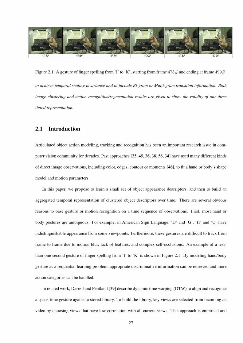
Figure 2.1: A gesture of finger spelling from ’I’ to ’K’, starting from frame 475# and ending at frame 499#.

to achieve temporal scaling invariance and to include Bi-gram or Multi-gram transition information. Both

image clustering and action recognition/segmentation results are given to show the validity of our three

tiered representation.

2.1 Introduction

Articulated object action modeling, tracking and recognition has been an important research issue in com-

puter vision community for decades. Past approaches [35, 45, 36, 38, 56, 34] have used many different kinds

of direct image observations, including color, edges, contour or moments [46], to fit a hand or body’s shape

model and motion parameters.

In this paper, we propose to learn a small set of object appearance descriptors, and then to build an

aggregated temporal representation of clustered object descriptors over time. There are several obvious

reasons to base gesture or motion recognition on a time sequence of observations. First, most hand or

body postures are ambiguous. For example, in American Sign Language, ’D’ and ’G’, ’H’ and ’U’ have

indistinguishable appearance from some viewpoints. Furthermore, these gestures are difficult to track from

frame to frame due to motion blur, lack of features, and complex self-occlusions. An example of a less-

than-one-second gesture of finger spelling from ’I’ to ’K’ is shown in Figure 2.1. By modeling hand/body

gesture as a sequential learning problem, appropriate discriminative information can be retrieved and more

action categories can be handled.

In related work, Darrell and Pentland [39] describe dynamic time warping (DTW) to align and recognize

a space-time gesture against a stored library. To build the library, key views are selected from incoming an

video by choosing views that have low correlation with all current views. This approach is empirical and

27

does not guarantee any sort of global consistency of the chosen views. As a result, recognition may be

unstable. In comparision, our method describes image appearances uniformly and clusters them globally

from a training set containing different gestures.

For static hand posture recognition, Tomasi et al. [57] apply vector quantization methods to cluster

images of different postures and different viewpoints. This is a feature-based approach, with thousands of

features extracted for each image. However, clustering in a high dimensional space is very difficult and can

be unstable. We argue that fewer, more global features are adequate for the purposes of gesture recognition.

Furthermore, the circular histogram representation has adjustable spatial resolution to accomodate differing

appearance complexities, and it is translation, rotation, and scale invariant.

In other work, [60, 41] recognize human actions at a distance by computing motion information between

images and relying on temporal correlation on motion vectors across sequences. Our work also makes use

of motion information, but does not rely exclusively on it. Rather, we combine appearance and motion cues

to increase sensitivity beyond what either can provide alone. Since our method is based on the temporal

aggregation of image clusters as a histogram to recognize an action, it can also be considered to be a temporal

texton-like method [121, 49]. One advantage of the aggregated histogram model in a time-series is that it

is straightforward to accommodate temporal scaling by using a sliding window. In addition, higher order

models corresponding to bigrams or trigrams of simpler “gestemes” can also be naturally employed to

extend the descriptive power of the method.

In summary, there are four principal contributions in this paper. First, we propose a new scale/rotation-

invariant hand image descriptor which is stable, compact and representative. Second, we introduce a meth-

ods for sequential smoothing of clustering results. Third, we show LDA/GMM with spectral partitioning

initialization is an effective way to learn well-formed probability densities for clusters. Finally, we recognize

image sequences as actions efficiently based on a flexible histogram model. We also discuss improvement

to the method by incorporating motion information.

28

Probabilistic Foreground Map (GMM Color Segmentation,

Probabilistic Appearance Modeling, Dynamic Texture Segmentation by

GPCA)

Feature Extraction via Circular/Fourier Representation

Feature Dimension Reduction via Variance Analysis

Framewise Clustering via Spectral Segmentation

(Initialization)

GMM/LDA Density Modeling for Clusters

Temporally Constrained Clustering (Refinement)

Temporal Aggregated Multiresolution Histogram for

Action

From Unigram to Bigram, Multigram Histogram Model

Temporal Pyramids and Scaling

Low Level: Rotation Invariant Feature Extraction

Intermediate Level: Clustering Presentation for Image Frames

High Level: Aggregated Histogram Model for Action Recognition

Figure 2.2: Diagram of a three tier approach for dynamic articulated object action modeling.

2.2 A Three Tiered Approach

We propose a three tiered approach for dynamic action modeling comprising low level feature extraction,

intermediate level feature vector clustering and high level histogram recognition as shown in Figure 2.2.

2.2.1 Low Level: Rotation Invariant Feature Extraction

In the low level image processing, our goals are to locate the region of interest in an image and to extract a

scale and in-plane rotation invariant feature vector as its descriptor. In order to accomplish this, a reliable and

stable foreground model of the target in question is expected. Depending on the circumstances, a Gaussian

mixture model (GMM) for segmentation [48], Maximum-Entropy color model ??, probabilistic appearance

modeling [37], or dynamic object segmentation by Generalized Principal Component Analysis (GPCA) [58]

are possible solutions. In this paper, we apply a GMM for hand skin color segmentation.

We fit a GMM by first performing a simple background subtraction to obtain a noisy foreground con-

taining a hand object (shown in Figure 2.3 (a)). From this, more than 1 million RGB pixels are used to train

skin and non-skin color density models with 10 Gaussian kernels for each class. Having done this, for new

images a probability density ratio Pskin/Pnonskin of these two classes is computed. If Pskin/Pnonskin is

larger than 1, the pixel is considered as skin (foreground) and is otherwise background. A morphological

operator is then used to clean up this initial segmentation and create a binary mask for the hand object.

29

0 10 20 30 40 50 60 700

0.5

1

1.5

2

2.5Inplane Rotation Invariant Image Feature Vector

Feature Number

Fea

ture

Mag

nitu

de

(a) (b) (c) (d)

Figure 2.3: (a) Image after background subtraction (b) GMM based color segmentation (c) Circular histogram for

feature extraction. (d) In-plane rotation invariant feature vector with 63 dimensions

We then compute the centroid and second central moments of this 2D mask. A circle is defined about the

target by setting its center as the centroid and its radius as 2.8 times largest eigenvalues of the second central

moment matrix (covering over 99% skin pixels in Figure 2.3 (c)). This circle is then divided to have 6 con-

centric annuli which contain 1, 2, 4, 8, 16, 32 bins from inner to outer, respectively. Since the position and

size of this circular histogram is determined by the color segmentation, it is translation and scale invariant.

We then normalize the density value Pskin + Pnonskin = 1 for every pixel within the foreground mask

(Figure 2.3) over the hand region. For each bin of the circular histogram, we calculate the mean of Pskin

( −log(Pskin), or −log(Pskin/Pnonskin) are also possible choices) of pixels in that bin as its value. The

values of all bins along each circle form a vector, and 1D Fourier transform is applied to this vector. The

power spectra of all annuli are ordered into a linear list producing a feature vector ~f(t) of 63 dimensions

representing the appearance of a hand image.1 Note that the use of the Fourier power spectrum of the annuli

makes the representation rotation invariant.

2.2.2 Intermediate Level: Clustering Presentation (Textons) for Image Frames

After the low level processing, we obtain a scale and rotation invariant feature vector as an appearance

representation for each image frame. The temporal evolution of feature vectors represent actions. However,

not all the images are actually unique in appearance. At the intermediate level, we cluster images from a set

of feature vectors. This frame-wise clustering is critical for dimension reduction and the stability of high1An optional dimension reduction of feature vectors can be achieved by eliminating dimensions which have low variance. It

means that feature values of those dimensions do not change much in the data, therefore are non-informative.

30

level recognition.

Initializing Clusters by Spectral Segmentation

There are two critical problems with clustering algorithms: determining the true number of clusters and

initializing each cluster. Here we use a spectral clustering method [135, 147, 59, 51] to solve both problems.

We first build the affinity matrix of pairwise distances between feature vectors2. We then perform a singular

value decomposition on the affinity matrix with proper normalization [135]. The number of clusters is deter-

mined by choosing the n dominant eigenvalues. The corresponding eigenvectors are taken as an orthogonal

subspace for all the data.

To get n cluster centers, we take the approach of [135] and choose vectors that minimize the absolute

value of cosine between any two cluster centers:

ID(k) =

rand(0, N)

if k = 1;

arg mint=1..N∑k−1

c=1 | cos( ~fn(ID(c)), ~fn(t))|

if n ≥ k > 1;

(2.1)

where ~fn(t) is the feature vector of image frame t after numerical normalization in [135] and ID(k) is

the image frame number chosen for the center of cluster k. N is the number of images used for spectral

clustering. For better clustering results, multiple restarts are used for initialization.

Unlike [51], we find this simple clustering procedure is sufficient to obtain a good set of clusters from

only a few restarts. After initialization, the Kmeans [5] is used to smooth the centers. Let C1(t) denote the

class label for image t, and ~g(c) = ~f(ID(c)); c = 1 . . . n denote cluster centers.

Refinement: Temporally Constrained Clustering

Spectral clustering methods are designed for an unordered “bag” of feature vectors, but, in our case, the

temporal ordering of image is an important source of information. In particular, the stability of appearance is2The exponent of either Euclidean distance or Cosine distance between two feature vectors can be used in this case.

31

easily computed by computing the motion energy3 between two frames. Let E(t) denote the motion energy

between frames t and t−1. Define Tk,j = t|C1(t) = k,C1(t−1) = j and E(k, j) =∑

t∈Tk,jE(t)/|Tk,j |.

We now create a regularized clustering cost function as

C2(t) = arg maxc=1..N

e−‖f(t)−g(c)‖

∑nc=1 e−‖f(t)−g(c)‖+

λe− ‖g(c)−g(C2(t−1))‖

E(t)

∑Nc=1 e

− ‖g(c)−g(C2(t−1))‖E(c,C2(t−1))

(2.2)

where λ is the weighting parameter. Here motion energy E(t) plays a role as the temperature T in simulated

annealing. When it is high (strong motion between frames), the motion continuity condition is violated

and the labels of successive frames can change freely; when it is low, the smoothness term constrains the

possible transitions of classes with low M(k, j).

With this in place, we now scan through the sequence searching for C2(t) of maximum value given

C2(t− 1) is already fixed. 4 This temporal smoothing is most relevant with images with motions, and static

frames are already stably clustered and therefore their cluster labels to not change.

GMM for Density Modeling and Smoothing

Given clusters, we build a probability density model for each. A Gaussian Mixture Model [43, 5] is used

to gain good local relaxation based on the initial clustering result provided by the above method and good

generalization for new data. Due to the curse of dimensionality, it is difficult to obtain a good estimate of

a high dimensional density function with limited and largely varied training data. We introduce an iterative

method incorporating Linear Discriminant Analysis (LDA) [5] and a GMM in an EM-like fashion to perform

dimensional reduction. The initial clustering labels help to build the scatter matrices for LDA. The optimal

projection matrix of LDA is then obtained from the decomposition of clusters’ scatter matrices [5]. The

original feature vectors can be further projected into a low dimensional space, which improves the estimation

of multi-variate Gaussian density function.3A simple method is to compute motion energy as the Sum of Squared Differences (SSD) by subtracting two Pskin density

masses from successive images.4Note that M(k, j) changes after scanning the labels of the image sequence once, thus more iterations could be used to achieve

more accurate temporal smoothness of C3(t), t = 1..N . From our experiments, more iterations does not change the result much.

32

With the new clustering result from GMM, LDA’s scatter matrices and projection matrix can be re-

estimated, and GMM can also be re-modeled in the new LDA subspace. This loop converges within 5 ∼

10 iterations from our experiments. Intuitively, LDA projects the data into a low dimensional subspace

where the image clusters are well separated, which helps to have a good parameter estimation for GMM

with limited data. Given more accurate GMM, more accurate clustering results are obtained, which also

causes better estimate of LDA. This Discriminative-GMM algorithm is described in the following and the

mathematical details are provided in the appendix. The algorithm includes 2 loops of iterations, the outer

loop of LDA-GMM and the inner loop of GMM’s EM process. Its experimental convergency is provided in

section 3.5, in terms of the log-likelihood and misclassification rate of both real and synthesized data. The

theoretical proof is currently undertaken. After this process, we have a Gaussian density model for each

cluster.

2.2.3 High Level: Aggregated Histogram Model for Action Recognition

Given a set of n clusters, define w(t) = [pc1(f(t)), pc2(f(t)), ..., pcn(f(t))]T where px(y) denotes the

density value of the vector y with respect to the GMM for cluster x. An action is then a trajectory of

[w(t1), w(t1 + 1), ..., w(t2)]T in Rn. For recognition purposes, we want to calculate some discriminative

statistics from each trajectory. One natural way is to use its mean Ht1,t2 =∑t2

t=t1w(t)/(t2−t1+1) over time

which is a temporal weighted histogram. Note that the histogram Ht1,t2 bins are precisely corresponding to

the trained clusters.

From the training set, we aggregate the cluster weights of images within a given hand action to form a

histogram model. In this way, a temporal image sequence corresponding to one action is represented by a

single vector. The matching of different actions is equivalent to compute the similarity of two histograms

which has variants. Here we use Bhattacharyya similarity metric [33] which has has several useful properties

including: it is an approximation of χ2 test statistics with fixed bias; it is self-consistent; it does not have the

singularity problem while matching empty histogram bins; and its value is properly bounded within [0, 1].

Assume we have a library of action histograms H∗1 , H∗

2 , ...,H∗M , the class label of a new action Ht1,t2 is

33

Discriminative-GMM Algorithm

inputs: Image Data X ; Labels L; Mixture Number

N

outputs: LDA Transform A; GMM Parameters

π, µ, Σ

1. Construct SW ;SB ⇐= X ;L.

2. Compute LDA Transform A ⇐=

LDA(SW ;SB), and project image data

X into the subspace Z = ATX with a lower

dimensions D.

3. Initialize GMM Parameters π, µ,Σ: πi =

1/N , Σi is aD dimensional identical matrix

where i = 1, 2, ...,N , and µi ⇐= Z;L

for the first time, while µi ⇐= Z;W for

others.

4. Learn GMM Parameters π, µ, Σ for Z via

Expectation-Maximization iterations.

(a) E-step: W ⇐= Z; π, µ,Σ

(b) M-step: π, µ,Σ ⇐= Z;W

5. Construct SW ;SB ⇐= X ;W.

6. Go to (2), until convergence.

determined by the following equation.

L(Ht1,t2) = arg minl=1..M

D(H∗l , Ht1,t2) =

[1−

n∑

c=1

√H∗

l (c) ∗ Ht1,t2(c)

] 12

(2.3)

34

This method is low cost because only one exemplar per action category is needed.

One problem with this method is that all sequence information has been compressed, e.g., we cannot dis-

tinguish an opening hand gesture from a closing hand using only one histogram. This problem can be easily

solved by subdividing the sequence and histogram model into m parts: Hmt1,t2 = [Ht1,(t1+t2)/m, ...,H(t1+t2)∗(m−1)/m,t2 ]

T .

For an extreme case when one frame is a subsequence, the histogram model simply becomes exactly the vec-

tor form of the representative surface.

We intend to classify hand actions with speed differences into the same category. To achieve this, the

image frames within a hand action can be sub-sampled to build a set of temporal pyramids. In order to

segment hand gestures from a long video sequence, we create several sliding windows with different frame

sampling rates. The proper time scaling magnitude is found by searching for the best fit over temporal

pyramids.

Taken together, the histogram representation achieves an adjustable multi-resolution measurement to

describe actions. A Hidden Markov Model (HMM) with discrete observations could be also employed

to train models for different hand actions, but more template samples per gesture class are required. The

histogram recognition method has the additional advantage that it does not depend on extremely accurate

frame-wise clustering. A small proportion of incorrect labels does not effect the matching value much. In

comparison, in an HMM with few training samples, outliers seriously impact the accuracy of learning. From

the viewpoint of considering hand actions as a language process, our model is an integration of individual

observations (by labelling each frame with a set of learned clusters) from different time slots. The labels’

transitions between successive frames are not used to describe the temporal sequence. By subdividing the

histogram, we are extending the representation to contain bigram, trigram, etc. information.

35

2.3 Results

2.3.1 Convergency of Discriminative-GMM.

We first show the convergency of our Discriminative-GMM algorithm by the increasing log-likelihood curve

of image data with the outer LDA-GMM iterations. In model selection literatures [5, 43], the model’s log-

likelihood is a monotonic function of the number of clusters M. In order to increase the log-likelihood

given the learnt model, we need to increase M. However we observe that the log-likelihood does increase

significantly within the first several LDA-GMM loops while both the mixture model size and the subspace

dimensions are fixed. We also generate 9 clusters of synthesized data with 5, 10, 15, 20, 25 dimensions. The

first 2 dimensions are shown in Figure 2.4 (b), and other dimensions are not distinguishable because they

are randomly sampled from the same normal distribution. Therefore, the optimal LDA projection should be

a 2 dimensional subspace close to the first 2 dimensions. Figure 2.4 (c,d) illustrate the convergency of the

LDA-GMM loops in terms of the improved log-likelihood and incorrect clustering ratios.

0 1 2 3 4 5 6 7 8 9 10 11 1220

25

30

35

40

45

50

55

Log−Likelihood of Clustering Data in the LDA−GMM Loops Image Number = 3050, Cluster Number = 24, Subspace Dimension = 10

Number of LDA−GMM Loops

Log−

Like

lihoo

d of

LD

A−

GM

M

−8 −6 −4 −2 0 2 4 6 8 10−8

−6

−4

−2

0

2

4

6

8The First 2 Dimensions of the Synthsized Data from 9 Clusters

class 1class 2class 3class 4class 5class 6class 7class 8class 9

1 2 3 4 5 6 7 8 9 107

7.5

8

8.5

9

9.5

Comparison of Log−Likelihood with synthesized data under different dimensions Image Number = 2700, Cluster Number = 9, Subspace Dimension = 2

Number of LDA−GMM Loops

Log−

Like

lihoo

d of

LD

A−

GM

M

Dimension = 5Dimension = 10Dimension = 15Dimension = 20Dimension = 25

1 2 3 4 5 6 7 8 9 100.05

0.1

0.15

0.2

0.25

0.3

0.35

0.4

Comparison of Clustering Error with synthesized data under different dimensions Image Number = 2700, Cluster Number = 9, Subspace Dimension = 2

Number of LDA−GMM Loops

Clu

ster

ing

Err

or R

atio

s of

LD

A−

GM

M

Dimension = 5Dimension = 10Dimension = 15Dimension = 20Dimension = 25

(a) (b) (c) (d)

Figure 2.4: (a) Log-likelihood of 3015 images with 24 clusters and 10 dimensional subspace (b) The first 2 dimensions

of the synthesized data from 9 clusters (c) Log-likelihood of the synthesized data of different dimensions (d) Ratios of

incorrect clustering of the synthesized data of different dimensions.

We have tested our three tiered method on the problem of recognizing sequences of hand spelling ges-

tures.

2.3.2 Framewise clustering.

We evaluate the low level representation of single images and intermediate clustering algorithms. A training

set of 3015 images are used. The frame-to-frame motion energy is used to label images as static or dynamic.

36

Figure 2.5: Image clustering results after low and intermediate level processing.

For spectral clustering, 3 ∼ 4 restarts from both the dynamic and static set are sufficient to cover all the

modes in the training set. Then, temporal smoothing is employed and a Gaussian density is calculated for

each cluster in a 10 dimensional subspace of the LDA projection. As a result, 24 clusters are obtained which

contain 16 static and 8 dynamic modes. Figure 2.5 shows 5 frames closest to the mean of the probability

density of cluster 1, 3, 19, 5, 13, 8, 21, 15, 6, 12. It can be seen that clustering results are insensitive to arti-

facts of skin segmentation. From Figure 2.5, it is also clear that dynamic modes have significantly larger

determinants than static ones. The study of the eigenvalues of covariance matrices shows that their super-

ellipsoid shapes are expanded within 2 ∼ 3 dimensions or 6 ∼ 8 dimensions for static or dynamic clusters.

Taken together, this means that static clusters are quite tight, while dynamic clusters contain much more

in-class variation. From Figure 2.6 (c), dynamic clusters gain more weight during the smoothing process

incorporating the temporal constraint and subsequent GMM refinement.

2.3.3 Action recognition and segmentation.

For testing images, we first project their feature vectors into the LDA subspace. Then, the GMM is used to

compute their weights with respect to each cluster. We manually choose 100 sequences for testing purposes,

and compute their similarities with respect to a library of 25 gestures. The length of the action sequences

37

A A

Y

Y A

A

Y

Y A

A

W

W A

A

A X

X A

(a) (b) (c) (d)

Figure 2.6: (a) Affinity matrix of 3015 images. (b) Affinity matrices of cluster centoids (from upper left to lower right) after

spectral clustering, temporal smoothing and GMM. (c) Labelling results of 3015 images (red squares are frames whose labels

changed with smoothing process after spectral clustering). (d) The similarity matrix of segmented hand gestures. The letters

are labels of gestures, for example, A −→ Y represents a sequence of gestures A −→ B, B −→ C,...,X −→ Y .

was 9 ∼ 38 frames. The temporal scale of actions in the same category ranged from 1 to 2.4. The results

were recognition rates of 90% and 93% without/with temporal smoothing (Equation 2.2). Including the top

three candidates, the recognition rates increase to 94% and 96%, respectively. We also used the learned

model and a sliding window with temporal scaling to segment actions from a 6034 frame video sequence

containing dynamic gestures and static hand postures. The similarity matrices among 123 actions found in

the video is shown in Figure 2.6 (d). 106 out of 123 actions (86.2%) are correctly segmented and recognized.

2.3.4 Integrating motion information.

As noted previously, our method cannot distinguish opening/closing hand gestures without temporally sub-

dividing histograms. An alternative solution is to integrate motion information5 between frames. Motion

feature vectors are also clustered, which results a joint (appearance and motion) histogram model for actions.

We assume independence of the data and therefore simple contatenate these two histograms into a single ac-

tion representation. From our preliminary experiments, both motion integration and histogram subdivision

are comparably effective to recognize gestures with opposite direction.5Motion information can be extracted by first aligning two hand blobs, subtracting two skin-color density masses, then using

the same circular histogram in section 2.1 to extract a feature vector for positive and negative density residues respectively. Another

simple way is to subtract two frames’ feature vectors directly.

38

2.4 Conclusion and Discussion

We have presented a method for classifying the motion of articulated gestures using LDA/GMM-based

clustering methods and a histogram-based model of temporal evolution. Using this model, we have obtained

extremely good recognition results using a relatively coarse representation of appearance and motion in

images.

There are mainly three methods to improve the performance of histogram-based classification, i.e., adap-

tive binning, adaptive subregion, and adaptive weighting [54]. In our approach, adaptive binning of the his-

togram is automatically learned by our clustering algorithms; adaptive subregion is realized by subdividing

action sequences to enrich the histogram’s descriptive capacity in the temporal domain; adaptive weighting

is achieved from the trained weights of Gaussian kernels in GMM.

Our future work will focus on building a larger hand action database containing 50 ∼ 100 categories for

more extensive testing, and on extending the representation to include other types of image information (e.g.

contour information). Also, by finding an effective foreground segmentation module, we intend to apply the

same methods to other applications such as recognizing stylized human body motion.

39

Chapter 3

Discriminative Learning of Spatial Image

Distribution:

A Two-level Image Spatial Representation

for Image Scene Category Recognition

Classifying pictures into one of several semantic categories is a classical image understanding problem.

In this paper, we present a stratified approach to both binary (outdoor-indoor) and multiple category of

scene classification. We first learn mixture models for 20 basic classes of local image content based on

color and texture information. Once trained, these models are applied to a test image, and produce 20

probability density response maps (PDRM) indicating the likelihood that each image region was produced

by each class. We then extract some very simple features from those PDRMs, and use them to train a bagged

random Linear Discriminant Analysis (LDA) classifier for 10 scene categories. For this process, no explicit

region segmentation or spatial context model are computed. To test this classification system, we created

a labeled database of 1500 home photos taken under very different environment and lighting conditions,

using different cameras, and from 43 persons over 5 years (1999-2004). The classification rate of outdoor-

40

indoor classification is 93.8%, and the classification rate for 10 scene categories is 90.1%. As a byproduct,

local image patches can be contextually labeled into the 20 basic material classes by using Loopy Belief

Propagation [167] as an anisotropic filter on PDRMs, producing an image-level segmentation if desired.

3.1 Introduction

Classifying pictures into semantic types of scenes [151, 158, 144] is a classical image understanding problem

which requires the effective interaction of high level semantic information and low level image observations.

Our goal is to build a very practical prototype for scene classification of typical consumer photos, along the

lines of the Kodak system [144]. Thus, we are interested in systems that are accurate, efficient, and which

can work with a wide range of photos and photographic quality.

Given the extremely large within-category variations in typical photographs, it is usually simpler and

thus easier to break the problem of scene classification into a two-step process. In this paper, we first train

local, image patch based color-texture Gaussian Mixture models (GMM) to detect each of 20 materials in

a local image patch. These models are used to scan an image and generate 20 local responses for each

pixel. Each response map, called a Probability Density Response Map (PDRM), can be taken as a real-

valued image indicating the relative likelihood of each material at each image location. We then compute

moments from the response maps and form a feature vector for each photo. By employing the random

subspace method [103, 162] and bootstrapping [165], we obtain a set of LDA scene classifiers over these

feature vectors. These classification results are combined into the final decision through bagging [68]. After

learning the local and global models, a typical 1200 × 800 image can be classified in less than 1 second

with our unoptimized Matlab implementation. Therefore there is a potential to develop a real-time scene

classifier upon our approach. A complete diagram of our approach is shown in Figure 3.1.

We organize the rest of the paper as follows. After a brief review of related previous published work, we

present the local image-level processing used to create PDRMs In section 3.3. Then in 3.4, we describe how

PDRMs are processed to perform scene classification. Experimental results and analysis on the performance

of patch based material detector and image based scene classification on a database of 1500 personal photos

41

image patches for blue sky

image patches for tree

image patches for pavement

Labeled Image Patches for each of 20 materials

Patch-based Discriminative Gaussian Mixture Density Model

for each of 20 materials

Patch B

ased Color-T

exture F

eature Extraction

LDA

Projection for M

aterial C

lasses

GMM for pavement

GMM for tree

GMM for blue sky

PDRM for pavement

PDRM for tree

PDRM for blue sky

Probability Density Response Maps for each of 20 materials

Mom

ents Feature E

xtraction and V

ectorization of Each P

DR

M

LDA

Projection for S

cene C

ategories (Bootstrapping+

Random

S

ubspace Sam

pling)

Bagging of LD

A C

lassifiers for S

cene Categories

Patch-Level Processing Image-Level Procesing

Figure 3.1: The diagram of our two level approach for scene recognition. The dashed line boxes are the input data or

output learned models; the solid line boxes represent the functions of our algorithm.

taken by 43 users using traditional or digital cameras over the last 5 years are given in section 3.5. Finally

we summarize the paper and discuss the future work in section 3.6.

3.2 Previous Work

There are several related efforts in this area. Luo et al. [127, 144] propose a bottom-up approach to first find

and label well-segmented image regions, such as water, beach, sky, and then to learn the spatial contextual

model among regions. A Bayesian network codes these relational dependencies. By comparison, we do not

perform an explicit spatial segmentation, and we use relatively simple (LDA-based) classification methods.

Perona et al. [83, 164] present a constellation model of clustered feature components for object recognition.

Their method works well for detecting single objects, but strongly depends on the performance and reliabil-

ity of the interest detector [110]. In the case of scene classification, we need to model more than one class

of material, where classes are non-structural and do not have significant features (such as foliage, rock and

et al.) [110]. This motivates our use of a GMM on the feature space. In order to maintain good stability,

we estimate the GMM in a linear subspace computed by LDA. These density models are quite flexible and

can be used to model a wide variety of image patterns with a good compromise between discrimination and

smoothness.

42

Kumar et al. [114, 115] propose the use of Markov random field (MRF)-based spatial contextual models

to detect man-made buildings in a natural landscape. They build a multi-scale color and textual descriptor

to capture the local dependence among building and non-building image blocks and use MRF to model

the prior of block labels. In our work, we have found that simple local labeling suffices to generate good

classification results; indeed regularization using loopy belief propagation method [167] yields no significant

improvement in performance. Thus, we claim that there is no need to segment image regions explicitly for

scene classification as other authors have done [144, 127, 115].

Linear discriminant analysis (LDA) is an optimization method to compute linear combinations of fea-

tures that have more power to separate different classes. For texture modeling, Zhu et al [169] pursue

features to find the marginal distributions which are also the linear combinations of the basic filter banks,

but they use a much more complex method (Monte Carlo Markov Chain) to stochastically search the space

of linear coefficients. In our case, the goal is not to build a generative model for photos belonging to dif-

ferent scenes, but simply to discriminate among them. We show a simple method such as LDA, if designed

properly, can be very effective and efficient to build a useful classifier for complex scenes.

3.3 Local Image-Level Processing

The role of image-level processing is to roughly classify local image content at each location in the image.

The general approach is to compute feature vectors of both color and texture, and then develop classifiers

for these features. In our current implementation, we have chosen to perform supervised feature classifica-

tion. Although arguably less practical than corresponding unsupervised methods, supervised classification

permits us to control the structure of the representations built at this level, and thereby to better understand

the relationship between low-level representations and overall system performance.

In this step, we compute 20 data driven probabilistic density models to describe the color-texture prop-

erties of image patches of 20 predefined materials1. These 20 categories are: building, blue sky, bush, other1The vocabulary of materials to be detected is designed by considering their popularity in the usual family photos. This definition

is, of course, not unique or optimized.

43

(mostly trained with human clothes), cloudy sky, dirt, mammal, pavement, pebble, rock, sand, skin, tree,

water, shining sky, grass, snow, carpet, wall and furniture.

To prepare the training data, we manually crop image regions for each material in our database, and

randomly draw dozens of 25 by 25 pixel patches from each rectangle. Altogether, we have 2000 image

patches for each material. Some examples of the cropped images and sampled image patches are shown in

Figure 3.2. For simplicity, we do not precisely follow the material boundaries in the photos while cropping.

Some outlier features are thus included in the training patches. Fortunately these outliers are smoothed

nicely by learning continuous mixture density models.

Figure 3.2: (a, c, e, g) Examples of cropped subimages of building, building under closer view, human skin, and grass

respectively. (b, d, f, h) Examples of image patches of these materials including local patches sampled from the above

subimages. Each local image patch is 25 by 25 pixels.

Multi-scale image representation and automatic scale selection problem has been a topic of intense

discussion over the last decade [125, 128, 110, 78, 114]. In general, the approach of most authors has been

to first normalize images with respect to the estimated scale of local image regions before learning. However

it is not a trivial problem to reliably recover the local image scales for a collection of 1500 family photos. We

instead choose to train the GMM using the raw image patches extracted directly from the original pictures.

For the labeled image patches with closer and coarser views, their complex color-texture distributions can

44

will be approximated by a multi-modal Gaussian mixture model during clustering.

3.3.1 Color-Texture Descriptor for Image Patches

Our first problem is to extract a good color-texture descriptor which effectively allows us to distinguish the

appearance of different materials. In the domain of color, experimental evaluation of several color models

has not indicated significant performance differences among color representations. As a result, we simply

represent the color of an image patch as the mean color in RGB space.

There are also several methods to extract texture feature vectors for image patches. Here we consider

two: filter banks, and the Haralick texture descriptor. Filter banks have been widely used for 2 and 3

dimensional texture recognition. [121, 76, 160]. We apply the Leung-Malik (LM) filter bank [121] which

consists of 48 isotropic and anisotropic filters with 6 directions, 3 scales and 2 phases. Thus, each patch is

represented by a 48 component feature vector.

The Haralick texture descriptor [98] is designed for image classification and has been adopted in the

area of image retrieval [61]. Haralick texture measurements are derived from the Gray Level Co-occurrence

Matrix (GLCM). GLCM is also called the Grey Tone Spatial Dependency Matrix which is a tabulation of

how often different combinations of pixel brightness values (grey levels) occur in an image region. GLCM

texture considers the relation between two pixels at a time, called the reference and the neighbor pixel. Their

spatial relation can be decided by two factors, the orientation and offset. Given any image patch, we search

all the pixel pairs satisfying a certain spatial relation and record their second order gray level distributions

with a 2 dimensional histogram indexed by their brightness values2. Haralick also designed 14 different

texture features [98] based on the GLCM. We selected 5 texture features including dissimilarity, Angular

Second Moment (ASM), mean, standard deviation (STD) and correction. Definitions for these can be found

in Appendix 6.1.

There is no general argument that the filter bank features or Haralick feature is a better texture descrip-

tor. We evaluate their texture discrimination performances experimentally in section 3.5 and find Haralick2The reference and neighbor pixel intensities normally need to be quantized into 16 or less levels instead of 256 which results

in not too sparse GLCM.

45

features generally perform better.

3.3.2 Discriminative Mixture Density Models for 20 Materials

The color and texture features for 2000 image patches form, in principle, an empirical model for each

material. However, classifying new patches against the raw features would require the solution to a high-

dimensional nearest-neighbor problem, and the result would be sensitive to noise and outliers. Instead, we

compute a continuous membership function using a Gaussian mixture model.

Although we have 2000 training samples, our feature vectors have 40 dimensions, so the training set is

still too sparse to learn a good mixture model without dimensional reduction. Because one of our purposes

is to maximize the discrimination among different materials, Linear Discriminant Analysis (LDA) [165]

was chosen to project the data into a subspace where each class is well separated. The LDA computation is

reviewed in appendix 6.2.

When each class has a Gaussian density with a common covariance matrix, LDA is the optimal trans-

form to separate data from different classes. Unfortunately the material color-texture distributions all have

multiple modes because the training image patches are sampled from a large variety of photos. Therefore

we have two options: employ LDA to discriminate among 20 material classes; or use LDA to separate all the

modes of materials. Although the latter seems closer to the model for which LDA was designed, we found

its material classification rate is worse because the optimal separation among the multiple modes within the

same material class is irrelevant. Therefore we choose the former.

The LDA computation provides a projection of the original feature space into a lower-dimensional fea-

ture spaceZ . We assume that the color-texture features of each material class is described by a finite mixture

distribution on Z of the form

P (z|c) =gc∑

k=1

πckG(z;µc

k, Σck), c = 1, 2, ..., 20 (3.1)

where the πck are the mixing proportions (

∑gc

k=1 πck = 1) and G(z;µc

k, Σck) is a multivariate Gaussian func-

tion depending on a parameter vector θck. The number of mixtures gc and the model parameters πc

k, θck

for each material class c are initialized by spectral clustering [135] and learned in an iterative Expectation-

46

Maximization manner [165, 40] where gc ranged from 4 to 8 depending on the material class. As a sum-

mary, discriminative Gaussian mixture models are obtained by applying LDA across the material classes

and learning the GMM within each material class, respectively.

3.4 Global Image Processing

3.4.1 Global Image Descriptor

Once we obtain 20 Gaussian mixture models πik, P (z; θi

k), i = 1, 2, ..., 20 for 20 material classes, we can

evaluate the membership density values of image patches for each material class. For any given photo, we

scan local image patches, extract their color-texture feature vector, normalize each of its components from 0

to 1 [61], project it to the lower dimensional subspaceZ computed by LDA, and finally compute the density

value given by equation (3.1) for all 20 material classes. The result is 20 real-valued grid maps3 representing

membership support for each of the 20 classes. An example is shown in Figure 3.3. Two examples of the

local patch labeling for indoor and outdoor photos are shown in Figure 3.4.

Figure 3.3: (a) Photo 1459#. (b) Its confidence map. (c, d, e, f, g) Its support maps of blue sky, cloud sky, water,

building and skin. Only the material classes with the significant membership support are shown.

Our next goal is to classify the photos into one of ten categories: cityscape, landscape, mountain, beach,

snow, other outdoors, portrait, party, still life and other indoor. In order to classify photos, we must still

reduce the dimension of the PDRMs to a manageable size. To do this, we compute the zeroth, first, and

second order moments of each PDRM. Intuitively, the zeroth moment describes the prevalence of a given

material class in an image; the first moment describes where it occurs, and the second moment its spatial

”spread”. The moment features from the 20 PDRMs are combined in a global feature vector Y.

3The size of the map depends on the original photo size and the patches’ spatial sampling intervals.

47

Skin

Skin

Bush

Furniture

Wall&Curtain

Pebbel

Blue Sky

Water

Pavement

Sand

Rock

Bush

Grass

Other

Building

(a) (b)

Figure 3.4: (a) The local patch material labeling results of an indoor photo. (b) The local patch material labeling

results of an outdoor photo. Loopy belief propagation is used for enhancement. The colored dots represent the

material label and the boundaries are manually overlayed for illustration purpose only.

3.4.2 Week Learner: LDA Classifers with Bootstrapping and Random Subspace Sampling

Using the scene category labels of the training photos, we now compute the LDA transform that attempts

to separate the training feature vectors of different categories. For the indoor-outdoor recognition, the LDA

projected subspace has only one dimension. As a typical pattern classification problem, we can find the

optimal decision boundary from the training data and apply it to the other testing data. Finding decision

boundaries for 10 scene category recognition is more complex. In practice, it is very difficult to train a

GMM classifier because of the data is too sparse over the 10 categories. As a result, we have used both the

nearest neighbor and Kmeans [165] classifiers for this decision problem.

We have found that the standard method for creating an LDA classifier works well for indoor-outdoor

scene classification, but the classification results for 10 scene categories is not good enough to constitute a

practical prototype. To improve the classification rate, we have implemented variations on random subspace

generation [103, 162] and bootstrapping [165] to create multiple LDA classifiers. These classifiers are

combined using bagging [68]. Recall that LDA is a two step process that first computes the singular value

decomposition (SVD) [90] of the within-class scatter matrix SW , then, after normalization, computes SVD

on the between-class scatter matrix S′B . After the first step, SW is divided into the principal subspace SP of

the nonzero eigenvalues ΛP and their associated eigenvectors UP , and the null subspace SN with the zero

eigenvalues ΛN and corresponding eigenvectors UN . In the traditional LDA transform, only SP is used for

the whitening of SW and normalization of SB while SN is discarded (see equation 6.18 in Appendix 6.2).

48

Chen et al. [72] have found that the null subspace SN satisfying UTP SW UP = 0 also contains important

discriminatory information. Here we make use of this observation by uniformly sampling an eigenvector

matrix Ur from UP ∪ UN and use it in place of U in the initial LDA projection step. Several projections

(including the original LDA projection matrix) are thus created.

In the second step of LDA, the subset VP of the full eigenvector matrix V with the largest eigenvalues,

normally replaces V in equation (6.18). It is also possible that there is useful discriminative information in

the subspace V − VP . Therefore we employ a similar sampling strategy as [162] in the context of PCA

by first sampling a small subset of eigenvectors Vr of V − VP , then replacing V with the joint subspace

VP ∪ Vr in equation 6.18.

Finally we also perform bootstrapping [165] by sampling subjects of the training set and creating LDA

classifiers for these subsets. By the above three random sampling processes, we learn a large set of LDA

subspaces and classifiers which we combine using the majority voting (bagging) methods [68]. In Section

3.5, we show the bagged recognition rates of 20 classifiers from bootstrapping replicates and 20 from random

subspace sampling.

3.5 Experiments

Our photo collection currently consists of 540 indoor and 860 outdoor customer photos. We randomly

select half of them as the training data and use other photos as the testing data. We have also intentionally

minimized redundancy when collecting photos, i.e., only one photo is selected when there are several similar

pictures.

3.5.1 Local Recognition: Validation of Image Patches Representation for Material Classes

We first address the problem of the image patch based color-texture feature description and classification.

Comparison of the recognition rates of 1200 testing image patches for each material class for different color-

texture descriptors, different numbers of training patches and different classifiers is provided in Figure 3.6

(a,b). In particular, we have also benchmarked the LDA+GMM model against a brute-force nearest neighbor

49

classifier. Let xj and zj represent an image patch feature vector before and after the LDA projection,

respectively. The nearest neighbor classifier computes the class label of a testing patch j as the label of that

training patch l such that ‖xj − xl‖ = mini‖xj − xi‖ where i ranges over the training image patches of

all material classes. The GMM classifier simply chooses the maximal class density, i.e. the class c∗ such

that P (zj |c∗) = maxc=1,2,...,20P (zj |c).

Comparing the plots shown in Figure 3.6, the classifier based on the Maximum Likelihood of GMM

density functions outperforms the Nearest Neighbor classifier, thus validating the use of the LDA+GMM

method. We also compared the recognition rates of 4 different feature combinations and found that the

Haralick texture descriptor combined with the mean color of the image patch yields the best results. Finally,

in Figure 3.6 (b), we see that the LDA+GMM method improves the recognition rate significantly when

increasing the training image patch from 500, becoming stable after 2000 patches.

Figure 3.5 shows the confusion rate using the GMM classifiers learned from 2000 training image patches

per class. The size of the white rectangle in each grid is proportional to the pairwise recognition error ratio.

The largest and smallest confusion rates are 23.6% and 0.24%, respectively. From Figure 3.5, we see that

pebble, rock and sand classes are well separated which shows that our patch-level learning process achieves

a good balance of Haralick texture and color cues by finding differences of the material classes with the

similar color. There is significant confusion among grass, bush and tree due to their similar color and texture

distribution. For some material classes, such as furniture, carpet, and other, the overall confusion rates are

also high.

3.5.2 Global Recognition: Photo based Scene Category Classification

For global classification, we have found that first order moment features of PRDMs are useful in outdoor

scenes, but reduce the recognition rate for indoor scenes. This makes sense since in most outdoor scenes

spatial contextual constraints, for instance the sky above grass, are useful cues. This naturally suggests a

hierarchical classification scheme (first determine indoor/outdoor followed by categorization), however we

have not yet pursued this approach. Thus, we confine ourselves to zeroth order moments for the remainder

50

building blue sky

bush

other c-sky

dirt

mammal pavement

pebble rock

sand skin

tree water

s-sky

grass snow

carpet

furniture wall

Figure 3.5: The pairwise confusion matrix of 20 material classes. The indexing order of the confusion

matrix is shown on the left of the matrix. The indexing order is symmetrical.

of this paper.

Our global image moment features after LDA projection are very easy to visualize in the indoor/outdoor

case as they become points in a 1-dimensional LDA subspace (3.6 (c)). In this case, the 1-D indoor-outdoor

decision boundary is simply determined by fitting a scaled exponential function to each of the indoor or

outdoor histogram distributions and calculating the point of intersection.

We show the recognition results of our method in Figure 3.6 (d), compared with the direct low-level

color or texture based scene recognition methods4 without LDA learning as the baselines. Our indoor-

outdoor recognition rate is 93.8%, which is comparable or slightly better than the Kodak’s recently pub-

lished classification system [144], although our approach is tested on a 40% larger photo database. It is

interesting that the bagging algorithm does not significantly improve the recognition performance of for

indoor-outdoor classification. The likely explanation is that the individual indoor-outdoor LDA classifiers

have nearly achieved the best possible recognition rate. Figure 3.7 shows 2 examples of misclassified pho-

tos. The first photo consists of a person sitting indoors, but in front of a curtain of tree leaves. In the second,

the playground is incorrectly classified as ”carpet” not ”dirt”. The appearance of people and animals are

irrelevant for indoor-outdoor classification — their associated moment features are assigned with near zero4We divide each image as a 9 by 9 grid, and extract the mean color or the DOG (Derivative of Gaussian) filtered texture features

within each grid. Each photo is then formulated as a feature vector by combining cues in all grids. A nearest neighbor classifier is

later employed for recognition based on the feature vectors’ distances of the training and testing photos.

51

500 1000 1500 2000 25000

0.1

0.2

0.3

0.4

0.5

0.6

0.7

0.8

0.9

1

Comparison of image patch recogniton of 4 features via Near−Neighbor Classifier

The number of training image patches

Rec

ogni

tion

rate

Filter BanksHaralickFilter Banks+ColorHaralick+Color

500 1000 1500 2000 25000

0.1

0.2

0.3

0.4

0.5

0.6

0.7

0.8

0.9

1

Comparison of image patch recogniton of 4 features via GMM Classifier

Rec

ogni

tion

rate

The number of training image patches

Filter BanksHaralickFilter Banks+ColorHaralick+Color

−6 −5 −4 −3 −2 −1 0 1 2 30

2

4

6

8

10

12

14

16

18

20

The Histogram of the LDA Features of the Trainging Indoor and Outdoor Photos in a One Dimensional Subspace

The Bins of the LDA Features

The

Num

ber

of P

hoto

s

indooroutdoor

(a) (b) (c)

0 5 10 15 20 25 30 35 400

0.1

0.2

0.3

0.4

0.5

0.6

0.7

0.8

0.9

1Comparison of Indoor−outdoor Scene Recognition

The Number of Classifiers

Rec

ogni

tion

Rat

e

Bagged LDA ClassifierRandom LDA ClassifiersColor based NN ClassifierTexture based NN Classifier

−8−6

−4−2

02

46

−6

−4

−2

0

2

4

6

−20

−10

0

10

Dimension One

The First 3 Dimensions of the Random Subspace LDA Features of 10 Scene Categories

Dimension Two

Dim

ensi

on T

hree

in1in2in3in4ot1ot2ot3ot4ot5ot6

0 5 10 15 20 25 30 35 400.7

0.72

0.74

0.76

0.78

0.8

0.82

0.84

0.86

0.88

0.9

Comparison of 10 Category Scene Recognition

The Number of Classifiers

Rec

ogni

tion

Rat

e

Bagged LDA Classifier with NNRandom LDA Classifiers with NNBagged LDA Classifier with KmeansRandom LDA Classifier with Kmeans

(d) (e) (f)

Figure 3.6: (a) Comparison of the image patch based recognition of 4 kinds of features (filter banks feature, Haralick

texture feature and their joint features with color) via Nearest-Neighbor Classifier. (b) Comparison of the image patch based

recognition of 4 kinds of features via GMM Classifier. (c)The 1D feature histogram distributions of indoor-outdoor photos

after LDA projection. (d) The comparison of indoor-outdoor recognition rates of 4 methods. (e) The first 3D feature point

distributions of 10 category photos after LDA projection. (f) The comparison of 10 categories recognition rates of 4 methods.

weights.

As shown in Figure 3.6 (e), feature points of some scene categories are well separated from others and

thus easy to be recognized in a certain LDA subspace, while some categories are not. Fortunately, Figure 3.6

(f) demonstrates that the individual LDA classifiers capture the complimentary discriminative information in

different random subspaces. Finally, it results that the combined (nearest neighbor and Kmeans) classifiers

both show improved performances of 6− 10% on average. As a comparison, Boutell et al. [66] achieve less

than 80% classification accuracy for 923 images in 5 categories. In their work, model-based graph matching

techniques are used to learn the explicit scene configuration consisting of semantic image regions.

52

(a) (b)

Figure 3.7: (a) An misclassified indoor photo. (b) An misclassified outdoor photo.

3.6 Conclusions & Discussion

This paper makes three contributions. First, we propose an efficient, yet effective, approach for scene recog-

nition for both indoor-outdoor and multiple photo categories. In practice, this approach can handle the

photos’ spatial complexity both in the local patch-level and the global image-level successfully. All the

training and testing processes are based upon a challenging photo database. Second, we describe a combi-

nation of LDA and Gaussian mixture models that achieves a good balance of discrimination and smoothness.

Finally, we study the use of moment features of PDRMs as an effective image-level representation for scene

classification, and the bagging [68] method to combine the individual scene classifiers obtained by the ran-

dom subspace algorithm [103]. The bagging method has shown success in our experiments, especially for

10 category scene recognition.

Although we have used supervised methods to create the local image patch classifiers, a practical sys-

tem would like learn at least some of these classifiers using unsupervised methods. However we believe

that the supervised material detectors provide the best scene recognition performance, and as such provide a

“benchmark” against which unsupervised methods can be evaluated. In future work, we intend to investigate

unsupervised clustering methods for low-level image patch classification. In particular, we plan to apply our

unsupervised, iterative LDA-GMM algorithm [?]. We also plan to investigate a hybrid approach where

classified images are used as labeled data to compute an initial LDA projection, which is then subsequently

refined with new, unlabeled images using iterative LDA-GMM. Finally, because LDA is only optimal when

each class has a Gaussian density with a common covariance matrix, the non-parametric discriminant analy-

sis (proposed in [168]) will be tested as a means to generalize our approach to a more comprehensive image

53

database which may contain thousands of various kinds of photos.

54

Chapter 4

Online Learning of Dynamic

Spatial-Temporal Image and Video

Appearance:

Matching, Segmenting and Tracking

Objects in Images and Videos using

Non-parametric Random Image Patch

Propagation

In this paper, we propose a novel exemplar-based approach to extract dynamic foreground regions from

a changing background within a collection of images or a video sequence. By using image segmentation

as a pre-processing step, we convert this traditional pixel-wise labeling problem into a lower-dimensional

supervised, binary labeling procedure on image segments. Our approach consists of three steps. First, a set

55

of random image patches are spatially and adaptively sampled within each segment. Second, these sets of

extracted samples are formed into two “bags of patches” to model the foreground/background appearance,

respectively. We perform a novel bidirectional consistency check between new patches from incoming frames

and current “bags of patches” to reject outliers, control model rigidity and make the model adaptive to new

observations. Within each bag, image patches are further partitioned and resampled to create an evolving

appearance model. Finally, the foreground/background decision over segments in an image is formulated

using an aggregation function defined on the similarity measurements of sampled patches relative to the

foreground and background models. The essence of the algorithm is conceptually simple and can be easily

implemented within a few hundreds of lines of Matlab code. We evaluate and validate the proposed approach

by extensive real examples of the object-level image mapping and tracking within a variety of challenging

environments. We also show that it is straightforward to apply our problem formulation on non-rigid object

tracking with difficult surveillance videos.

4.1 Introduction

In this paper, we study the problem of object-level figure/ground segmentation in images and video se-

quences. The core problem can be defined as follows: Given an image X with known figure/ground labels

L, infer the figure/ground labels L′ of a new image X′ closely related to X. For example, we may want

to extract a walking person in an image using the figure/ground mask of the same person in another image

of the same sequence. Our approach is based on training a classifier from the appearance of a pixel and

its surrounding context (i.e., an image patch centered at the pixel) to recognize other similar pixels across

images. To apply this process to a video sequence, we also evolve the appearance model over time.

A key element of our approach is the use of a prior segmentation to reduce the complexity of the seg-

mentation process. As argued in [138], image segments are a more natural primitive for image modeling

than pixels. More specifically, an image segmentation provides a natural dimensional reduction from the

spatial resolution of the image to a much smaller set of spatially compact and relatively homogeneous re-

gions. We can then focus on representing the appearance characteristics of these regions. Borrowing a term

56

from [138], we can think of each region as a ”superpixel” which represents a complex connected spatial

region of the image using a rich set of derived image features. We can then consider how to classify each

superpixel (i.e. image segment) as foreground or background, and then project this classification back into

the original image to create the pixel-level foreground-background segmentation we are interested in.

The original superpixel representation in [138, 129, 128] is a feature vector created from the image

segment’s color histogram [129], filter bank responses [138], oriented energy [128] and contourness [128].

These features are effective for image segmentation [128], or finding perceptually important boundaries

from segmentation by supervised training [138]. However, as shown in [11], those parameters do not work

well for matching different classes of image regions from different images. Instead, we propose using a

set of spatially randomly sampled image patches as a non-parametric, statistical superpixel representation.

This non-parametric “bag of patches” model1 can be easily and robustly evolved with the spatial-temporal

appearance information from video, while maintaining the model size (the number of image patches per

bag) using adaptive sampling. Foreground/background classification is then posed as the problem of match-

ing sets of random patches from the image with these models. Our major contributions are demonstrating

the effectiveness and computational simplicity of a nonparametric random patch representation for seman-

tically labelling superpixels and a novel bidirectional consistency check and resampling strategy for robust

foreground/background appearance adaptation over time.

We organize the paper as follows. We first address the related work in the areas of computer vision

and graphics. Then several image patch based representations and the associated matching methods are

described. In section 4.4, the algorithm used in our approach is presented with details. We demonstrate

the validity of the proposed approach using experiments on real examples of the object-level figure/ground

image mapping and non-rigid object tracking under dynamic conditions from videos of different resolutions

in section 4.5. Finally, we summarize the contributions of the paper and discuss possible extensions and

improvements.1Highly distinctive local features [126] are not the adequate substitutes for image patches. Their spatial sparseness nature

limits their representativity within each individual image segment, especially for the nonrigid, nonstructural and flexible fore-

ground/backgroung appearance.

57

(a) (b) (c) (d)

Figure 4.1: (a) An example indoor image, (b) the segmentation result using [82] coded in ran-

dom colors, (c) the boundary pixels between segments shown in red, the image segments as-

sociated with the foreground, a walking person here, shown in blue, (d) the associated fore-

ground/background mask. Notice that the color in (a) is not very saturated. This is a common fact

in our indoor experiments without any specific lighting controls.

4.2 Related work

In this paper, we propose a simple nonparametric random patch treatment unifying supervised semantic ob-

ject segmentation across images, non-rigid object segmentation tracking in moderate/high resolution videos

and temporal small object localization in low resolution videos. All these tasks involve a non-rigid figure

object, a moving camera or a changing background. We show real examples in a variety of conditions which

are related to a wide range of previous work as follows.

Most previous work on foreground/background extraction are based on the pixel-level processing of im-

ages from static cameras using color as the primary feature [73, 139, 123, 124, 161, 133, 146]. Image patch

based appearance modeling [80, 121, 11] and matching enriches both the descriptive and discriminative

abilities for figure/ground classification compared to the pixel-color representation. Patch based image sam-

pling and matching has shown great success in texture synthesis [80], texture recognition [121] and superior

performance in object recognition [?] than image features [126].

Interactively extracting a foreground object from an image [139, 123], or segmenting a moving object

from a video sequence [124, 161] remains a difficult computer graphics task. The state-of-the-art [139,

123, 124, 161] employ an interactive graph-cut algorithm [67] as a Markov random field solver to assign

pixels with figure/ground labels using color cues. It normally needs huge amount of manual interactions and

assumes the camera pose is simply fixed. Our paper attempts to provide an automatic means to propagate

58

supervised semantic segmentation labels over images by nonparametric appearance modeling and temporal-

spatial video frames.

Li et al. [123] and Rother et al. [139] utilized an interactive graph-cut algorithm [67] as a Markov

random field solver to assign pixels with figure/ground labels. Li et al. [124] further extended this approach

to video cutout applications using a 3D graph-cut algorithm on the spatial-temporal space. Most work is

primarily based on color, and video cutout papers [124, 161] assume that the background is static.

Dynamically changing backgrounds render many of the above methods ineffective. In recent work,

[146, 133] describe pixel-wise foreground detection algorithms to handle a quasi-static2 background. This

work relies on a local smoothing process on the pixels occupied by dynamic textures using a kernel density

estimator in the joint spatial-color space. However, the approach does not handle the change in background

due to a moving camera. Motion segmentation is another approach to find independent moving objects

by computing an exact model of background motion [?]. Unfortunately it is only effective for segmenting

small moving objects from a constrained dominant background motion, mostly for aerial visual surveil-

lance applications. By comparison, our treatment of image segments (instead of pixels) as the elements of

foreground/background classification avoids the need for motion assumptions across images.

The idea of using ”superpixels” as the representative elements for object-level image mapping is inspired

by [138, 129, 123, 105]. For moderate resolution images, the number of segments in a segmentation is typ-

ically several orders of magnitude lower than the number of pixels. This makes the foreground/background

extraction problem computationally more tractable. Also, as we will show, moderately rigid or non-rigid

spatial transforms of figure/ground across images tend not to affect our segment-based classification. As a

result, there is no reliance on a figure/ground motion or shape model. Our non-parametric statistical appear-

ance representation of superpixel is in the same spirit of [80]. They employ it to synthesize textures, while

we use it for segment-based foreground/background labelling. Recently, [?] proposes a hierarchical model

switching method for unsupervised video segmentation which involves variational inference over many con-

ditional switching and conditional hidden variables. It is very computationally expensive (thus feasible for2A static scene with periodically changing objects, such as a running river, waving trees, or ocean waves and so on.

59

limited low resolution videos only), and depends highly on a complex switching process among different

global shape/appearance models.

We also extend our nonparametric formulation of random patches into tracking non-rigid interested ob-

jects from surveillance videos, and compared it with the state-of-the-art [?, 96]. [96] utilizes meanshift mode

seeking [?] to maintain an online appearance-changing Gaussian mixture density model. The meanshift den-

sity model has potential difficulties for high dimensional image features that limit its descriptiveness. [?]

employs Adaboosting to obtain an ensemble of recently trained weak classifiers for the temporal appearance

model updating and classification. This approach loses the original format of image patch appearance and

restricts to boosting for classification. Instead of using boosting as in [?], our approach has a novel bidi-

rectional check and resampling strategy to keep the figure/ground dynamic appearance model robust and

updated along time. As we show later, the strategy only involves simple computations with flexible and

controllable descriptive ability while naturally combining long-term and short-term appearance samples. It

also leaves the classification process with freedom to choose over different classifiers.

4.3 Image Patch Representation and Matching

Building stable appearance representations of images patches is fundamental to our approach. There are

many derived features that can be used to represent the appearance of an image patch. In this paper, we

evaluate our algorithm based on: 1) an image patch’s raw RGB intensity vector, 2) mean color vector,

3) color + texture descriptor (filter bank response or Haralick feature [11]), and 4) PCA, LDA and NDA

(Nonparametric Discriminant Analysis) features [87, 69] on the raw RGB vectors. For completeness, we

give a brief description of each of these techniques.

4.3.1 Texture descriptors

To compute texture descriptions, we first apply the Leung-Malik (LM) filter bank [121] which consists of

48 isotropic and anisotropic filters with 6 directions, 3 scales and 2 phases. Thus each image patch is

represented by a 48 component feature vector. The Haralick texture descriptor [98] was used for image

60

classification in [11]. Haralick features are derived from the Gray Level Co-occurrence Matrix, which is

a tabulation of how often different combinations of pixel brightness values (grey levels) occur in an image

region. We selected 5 out of 14 texture descriptors [98] including dissimilarity, Angular Second Moment

(ASM), mean, standard deviation (STD) and correlation. For details, refer to [98, 11].

4.3.2 Dimension reduction representations

The Principal Component Analysis (PCA) algorithm is used to reduce the dimensionality of the raw color

intensity vectors of image patches. PCA makes no prior assumptions about the labels of data. However,

recall that we construct the ”bag of patches” appearance model from sets of labelled image patches. This

supervised information can be used to project the bags of patches into a subspace where they are best sepa-

rated using Linear discriminant Analysis (LDA) or Nonparametric Discriminant Analysis (NDA) algorithm

[87, 69] by assuming Gaussian or Non-Gaussian class-specific distributions.

Comparison of LDA and NDA

Both NDA and LDA compute an optimal projection matrix W based on the within-class and between-class

scatter matrices SW , SB3, by maximizing the intra-class separation W T SBW/W T SW W. When each

class has a Gaussian density with a common covariance matrix, LDA is the optimal discriminative trans-

form to separate data from different classes. However the image patches of foreground/background classes

usually have very complex multimodal distributions. The nonparametric nature of scatter matrices SW , SB

in NDA [87, 69] can inherently lead to extract projected features that preserve relevant complex structures

of classification. However, through our experiments, the nonlinear separatibility of different classes in the

NDA projected subspace is very sensitive to its parameter settings while building scatter matrices. There is

no principal way or computationally intractable to find optimal parameters for arbitrary complex distribu-

tions.

NDA differs from LDA in how it constructs SW , SB matrices. For each image patch p, we need to find3SW is the covariance matrix of data to its intra-class mean; SB is the covariance matrix of the intra-class means to the overall

mean.

61

the means pI , pE of its nearest neighbor sets pI, pE from both the intra-class and inter-class patch bags.

This can be computationally expensive with the large size bags of patches and the high dimensionality of

the image patch. In this paper, we cluster image patches within each bag (as described in section 4.4.4)

and use the cluster centers to find approximations of pI , pE as follows. Given the center sets CF , CB ,

any foreground image patch’s intra-class mean is chosen as c ∈ CF within the same partition and its inter-

class mean is c ∈ CB with the minimal distance; similarly for background patches. Then SW , SB are

constructed as covariance matrices using these local means [69]. The computational complexity decreases

from O(N2d) to O(kNd) where N image patches are clustered into k partitions and d is the patch feature

vector’s dimensionality. After constructing the parametric or non-parametric scatter matrices SW , SB , both

LDA and NDA can be solved as a generalized eigenvalue problem [5]. For details, refer to [87, 69].

4.3.3 Patch matching

: After image patches are represented using one of the above methods, we must match them against the fore-

ground/background models. There are 2 methods investigated in this paper: the nearest neighbor matching

using Euclidean distance and KDE (Kernel Density Estimation) [106] in PCA/NDA subspaces. For nearest-

neighbor matching, we find, for each patch p, its nearest neighbors pFn , pB

n in foreground/background bags,

and then compute dFp =‖ p − pF

n ‖, dBp =‖ p − pB

n ‖. On the other hand, an image patch’s matching

scores mFp and mB

p are evaluated as probability density values from the KDE functions KDE(p,ΩF ) and

KDE(p, ΩB) where ΩF |B are bags of patch models. Then the segmentation-level classification is per-

formed as section 4.4.3.

4.4 Algorithms

We briefly summarize our labeling algorithm as follows. We assume that each image of interest has been

segmented into spatial regions. A set of random image patches are spatially and adaptively sampled within

each segment. These sets of extracted samples are formed into two “bags of patches” to model the fore-

ground/background appearance respectively. The foreground/background decision for any segment in a new

62

image is computed using one of two aggregation functions on the appearance similarities from its inside

image patches to the foreground and background models. Finally, for videos, within each bag, new patches

from new frames are integrated through a robust bidirectional consistency check process and all image

patches are then partitioned and resampled to create an evolving appearance model. As described below,

this process prune classification inaccuracies in the nonparametric image patch representations and adapts

them towards current changes in foreground/background appearances for videos.

4.4.1 Algorithm Diagram

We describe each of these steps for video tracking of foreground/background segments in more detail below,

and for image matching, which we treat as a special case by simply omitting step 3 and 4 in Figure 4.2.

4.4.2 Sample Random Image Patches

We first employ an image segmentation algorithm4 [82] to pre-segment all the images or video frames

in our experiments. A typical segmentation result is shown in Figure 4.1. We use Xt, t = 1, 2, ..., T

to represent a sequence of video frames. Given an image segment, we formulate its representation as a

distribution on the appearance variation over all possible extracted image patches inside the segment. To

keep this representation to a manageable size, we approximate this distribution by sampling a random subset

of patches.

We denote an image segment as Si with SFi for a foreground segment, and SB

i for a background segment,

where i is the index of the (foreground/background)image segment within an image. Accordingly, Pi, PFi

and PBi represent a set of random image patches sampled from Si, SF

i and SBi respectively. The cardinality

Ni of an image segment Si generated by [82] typically ranges from 50 to thousands. However small or

large superpixels are expected to have roughly the same amount of uniformity. Therefore the sampling rate

γi of Si, defined as γi = size(Pi)/Ni, should decrease with increasing Ni. For simplicity, we keep γi as

a constant for all superpixels, unless Ni is above a predefined threshold τ , (typically 2500 ∼ 3000), above4Because we are not focused on image segmentation algorithms, we choose Felzenszwalb’s segmentation code which generates

good results and is publicly available at http://people.cs.uchicago.edu/∼pff/segment/.

63

Non-parametric Patch Appearance Modelling-Matching Algorithm

inputs: Pre-segmented Images Xt, t = 1, 2, ..., T ; Label L1

outputs: Labels Lt, t = 2, ..., T ; 2 “bags of patches” appearance model for fore-

ground/background ΩF |BT

1. Sample segmentation-adaptive random image patches P1 from image X1.

2. Construct 2 new bags of patches ΩF |B1 for foreground/background using patches P1

and label L1; set t = 1.

3. t = t + 1; Sample segmentation-adaptive random image patches Pt from image Xt;

match Pt with ΩF |Bt−1 and classify segments of Xt to generate label Lt by aggregation.

4. Classify and reject ambiguous patch samples, probable outliers and redundant appear-

ance patch samples from new extracted image patches Pt against ΩF |Bt−1 ; Then inte-

grate the filtered Pt into ΩF |Bt−1 and evaluate the probability of survival ps for each

patch inside ΩF |Bt−1 against the original unprocessed Pt (Bidirectional Consistency

Check).

5. Perform the random partition and resampling process according to the normalized prod-

uct of probability of survival ps and partition-wise sampling rate γ′ inside ΩF |Bt−1 to

generate ΩF |Bt .

6. If t = T , output Lt, t = 2, ..., T and ΩF |BT ; exit. If t < T , go to (3).

Figure 4.2: Non-parametric Patch Appearance Modelling-Matching Algorithm

which size(Pi) is held fixed. This sampling adaptivity is illustrated in Figure 4.3. Notice that large image

segments have much more sparsely sampled patches than small image segments. From our experiments,

this adaptive spatial sampling strategy is sufficient to represent image segments of different sizes.

4.4.3 Label Segments by Aggregating Over Random Patches

For an image segment Si from a new frame to be classified, we again first sample a set of random patches

Pi as its representative set of appearance samples. For each patch p ∈ Pi, we calculate its distances dFp , dB

p

or matching scores mBp ,mF

p towards the foreground and background appearance models respectively as

64

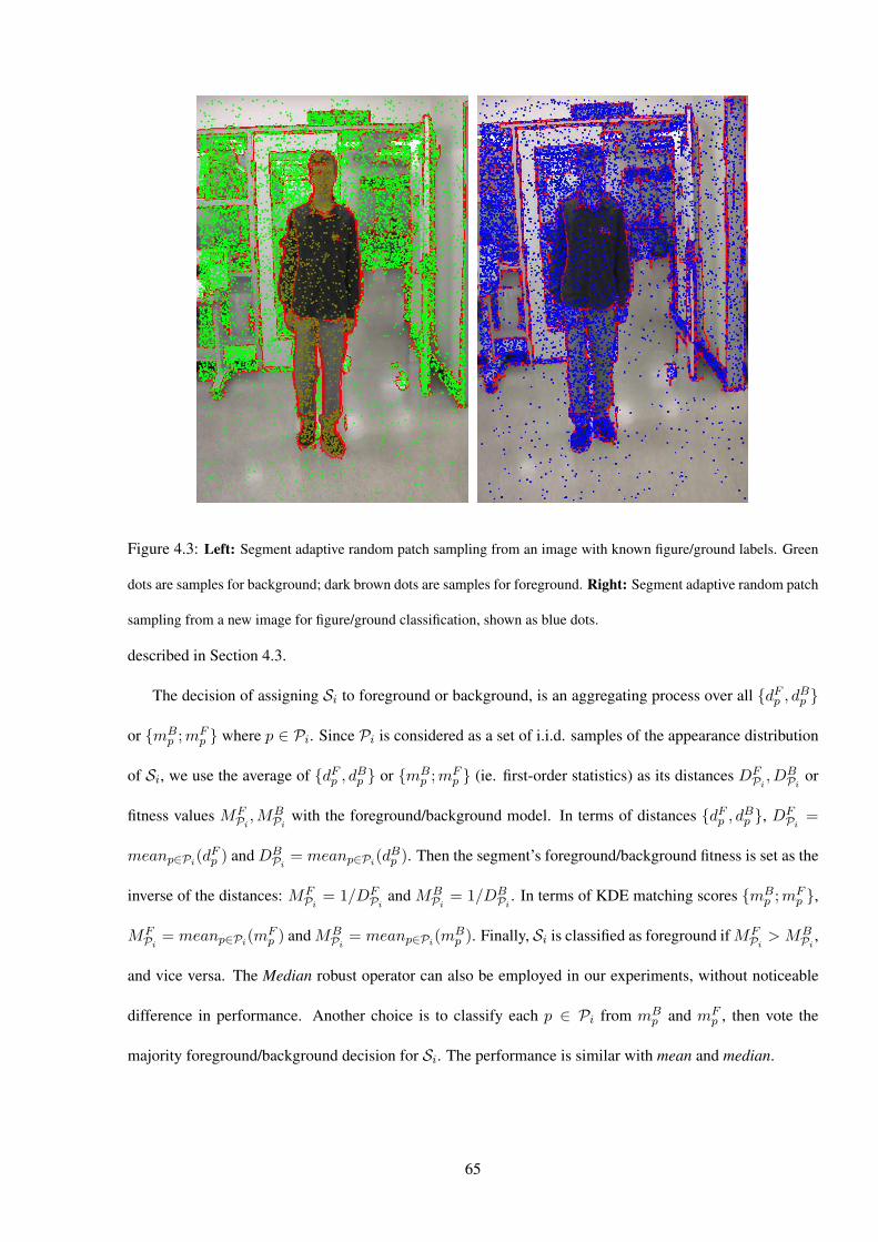
Figure 4.3: Left: Segment adaptive random patch sampling from an image with known figure/ground labels. Green

dots are samples for background; dark brown dots are samples for foreground. Right: Segment adaptive random patch

sampling from a new image for figure/ground classification, shown as blue dots.

described in Section 4.3.

The decision of assigning Si to foreground or background, is an aggregating process over all dFp , dB

p

or mBp ; mF

p where p ∈ Pi. Since Pi is considered as a set of i.i.d. samples of the appearance distribution

of Si, we use the average of dFp , dB

p or mBp ; mF

p (ie. first-order statistics) as its distances DFPi

, DBPi

or

fitness values MFPi

,MBPi

with the foreground/background model. In terms of distances dFp , dB

p , DFPi

=

meanp∈Pi(dFp ) and DB

Pi= meanp∈Pi(d

Bp ). Then the segment’s foreground/background fitness is set as the

inverse of the distances: MFPi

= 1/DFPi

and MBPi

= 1/DBPi

. In terms of KDE matching scores mBp ; mF

p ,

MFPi

= meanp∈Pi(mFp ) and MB

Pi= meanp∈Pi(m

Bp ). Finally, Si is classified as foreground if MF

Pi> MB

Pi,

and vice versa. The Median robust operator can also be employed in our experiments, without noticeable

difference in performance. Another choice is to classify each p ∈ Pi from mBp and mF

p , then vote the

majority foreground/background decision for Si. The performance is similar with mean and median.

65

4.4.4 Construct a Robust Online Nonparametric Foreground/Background Appearance Model

with Temporal Adaptation

From sets of random image patches extracted from superpixels with known figure/ground labels, 2 fore-

ground/background “bags of patches” are composed. The bags are the non-parametric form of the fore-

ground/background appearance distributions. When we intend to “track” the figure/ground model sequen-

tially though a sequence, these models need to be updated by integrating new image patches extracted from

new video frames. However the size (the number of patches) of the bag will be unacceptably large if we

do not also remove the some redundant information over time. More importantly, imperfect segmentation

results from [82] can cause inaccurate segmentation level figure/ground labels. For robust image patch level

appearance modeling of Ωt, we propose a novel bidirectional consistency check and resampling strategy to

tackle various noise and labelling uncertainties.

More precisely, we classify new extracted image patches Pt as PFt or PB

t according to ΩF |Bt−1 ;

and reject ambiguous patch samples whose distances dFp , dB

p towards respective ΩF |Bt−1 have no good contrast

(simply, the ratio between dFp and dB

p falls into the range of 0.8 to 1/0.8). We further sort the distance list of

the newly classified foreground patches PFt to ΩF

t−1, filter out image patches on the top of the list which

have too large distances and are probably to be outliers, and ones from the bottom of the list which have too

small distances and contain probably redundant appearances compared with ΩFt−1

5. We perform the same

process with PBt according to ΩB

t−1. Then the filtered Pt are integrated into ΩF |Bt−1 to form ΩF ′|B′

t−1 , and

we evaluate the probability of survival ps for each patch inside ΩF ′|B′t−1 against the original unprocessed Pt

with their labels6.

Next, we cluster all image patches of ΩF ′|B′t−1 into k partitions [91], and randomly resample image patches

within each partition. This is roughly equivalent to finding the modes of an arbitrary distribution and sam-5Simply, we reject patches with distances dF

pFt

that are larger than mean(dFpF

t) + λ ∗ std(dF

pFt

) or smaller than mean(dFpF

t)−

λ ∗ std(dFpF

t) where λ controls the range of accepting patch samples of Ω

F |Bt−1 , called model rigidity.

6For example, we compute the distance of each patch in ΩF ′t−1 to PF

t , and covert them as surviving probabilities using a

exponential function over negative covariance normalized distances. Patches with smaller distances have higher survival chances

during resampling; and vice versa. We perform the same process with ΩB′t−1 according to PB

t .

66

pling for each mode. Ideally, the resampling rate γ′ should decrease with increasing partition size, similar

to the segment-wise sampling rate γ. For simplicity, we define γ′ as a constant value for all partitions,

unless setting a threshold τ ′ to be the minimal required size7 of partitions after resampling. If we perform

resampling directly over patches without partitioning, some modes of the appearance distribution may be

mistakenly removed. This strategy represents all partitions with sufficient number of image patches, regard-

less of their different sizes. In all, we resample image patches of ΩF |Bt−1 , according to the normalized product

of probability of survival ps and partition-wise sampling rate γ′, to generate ΩF |Bt . By approximately fixing

the expected bag model size, the number of image patches extracted from a certain frame Xt in the bag

decays exponentially in time.

The problem of partitioning image patches in the bag can be formulated as the NP-hard k-center problem.

The definition of k-center is as follows: given a data set of n points and a predefined cluster number k, find

a partition of the points into k subgroups P1,P2, ...,Pk and the data centers c1, c2, ..., ck, to minimize the

maximum radius of clusters maxi maxp∈Pi ‖ p − ci ‖, where i is the index of clusters. Gonzalez [91]

proposed an efficient greedy algorithm, farthest-point clustering, which proved to give an approximation

factor of 2 of the optimum. The algorithm operates as follows: pick a random point p1 as the first cluster

center and add it to the center set C; for iterations i = 2, ..., k, find the point pi with the farthest distance to

the current center set C: di(pi, C) = minc∈C ‖ pi − c ‖ and add pi to set C; finally assign data points to its

nearest center and recompute the means of clusters in C. Compared with the popular k-means algorithm, this

algorithm is computationally efficient and theoretically bounded8. In this paper, we employ the Euclidean

distance between an image patch and a cluster center, using the raw RGB intensity vector or the feature

representations discussed in section 4.3.7All image patches from partitions that are already smaller than τ ′ are kept during resampling.8The random initialization of all k centers and the local iterative smoothing process in k-means, which is time-consuming in

high dimensional space and possibly converges to undesirable local minimum, are avoided.

67

4.5 Experiments

We have evaluated the image patch representations described in Section 4.3 for figure/ground mapping

between pairs of image on video sequences taken with both static and moving cameras. Here we summarize

our results.

4.5.1 Evaluation on Object-level Figure/Ground Image Mapping

We first evaluate our algorithm on object-level figure/ground mapping between pairs of images under eight

configurations of different image patch representations and matching criteria. They are listed as follows:

the nearest neighbor distance matching on the image patch’s mean color vector (MCV); raw color intensity

vector of regular patch scanning (RCV) or segment-adaptive patch sampling over image (SCV); color + filter

bank response (CFB); color + Haralick texture descriptor (CHA); PCA feature vector (PCA); NDA feature

vector (NDA) and kernel density evaluation on PCA features (KDE). In general, 8000 ∼ 12000 random

patches are sampled per image. There is no apparent difference on classification accuracy for the patch size

ranging from 9 to 15 pixels and the sample rate from 0.04 to 0.10. The PCA/NDA feature vector has 20

dimensions, and KDE is evaluated on the first 3 PCA features.

Because the foreground figure has fewer of pixels than background, we conservatively measure the

classification accuracy from the foreground’s detection precision and recall on pixels. Precision is the ratio

of the number of correctly detected foreground pixels to the total number of detected foreground pixels;

recall is is the ratio of the number of correctly detected foreground pixels to the total number of foreground

pixels in the image.

The patch size is 11 by 11 pixels, and the segment-wise patch sampling rate γ is fixed as 0.06. Using 40

pairs of (720×480) images with the labelled figure/ground segmentation, we compare their average running

time and classification accuracies in Tables 4.1 and 4.2. All the algorithms are implemented under Matlab

6.5 on a P4-1.8G PC.

The nearest neighbor matching has computational complexity O(N2d) where N is the number of sam-

pled patches per image and d is the dimensionality of the image patch representation. Therefore the running

68

MCV RCV SCV CFB CHA PCA NDA KDE

0.9 8.5 4.5 2.2 2.6 1.2 1.6 0.38

Table 4.1: Evaluation on running time (minutes).

MCV RCV SCV CFB CHA PCA NDA KDE

0.46 0.81 0.97 0.92 0.89 0.93 0.96 0.69

0.28 0.89 0.95 0.85 0.81 0.85 0.87 0.98

Table 4.2: Evaluation on classification accuracy (ratio). The first row is precision; the second row is recall.

time differences of MCV, RCV, SCV, CFB, CHA, PCA, NDA mostly depend on d, except for the extra ex-

pense of feature extraction for CFB, CHA, PCA, NDA. Given an 11 by 11 pixel image patch, its raw RGB

intensity vector has 363 dimensions. The dimensionality of color-texture descriptor is 51 for LM filter bank

and 43 for Haralick texture features. The PCA and NDA features have dimensionalities ranging from 5

to 40 with comparable classification accuracy. KDE Matlab toolbox [106] uses tree-based approximations

on kernel evaluation which boosts its speed. For figure/ground extraction accuracy, SCV has the best clas-

sification ratio using the raw color intensity vector without any dimension reduction. MCV has the worst

accuracy, which shows that pixel-color leads to poor separability between figure and ground in our data set.

Four feature based representations, CFB, CHA, PCA, NDA with reduced dimensions, have similar perfor-

mance, whereas NDA is slightly better than the others. KDE tends to be more biased towards the foreground

class because background usually has a wider, flatter density distribution. The superiority of SCV over RCV

proves that our segment-wise random patch sampling strategy is more effective at classifying image seg-

ments than regularly scanning the image, even with more samples. As shown in Figure 4.4 (b), some small

or irregularly-shaped image segments do not have enough patch samples to produce stable classifications.

To allow a more intuitive understanding the evaluation results, we present a set of example images

with the detected figure segments in blue and their white/black masks in Figure 4.4. Another example of

figure/ground mapping results from surgical images is illustrated in Figure 4.6. Our approach successfully

distinguishes the extracted foreground object from another surgical tool with very similar appearance in the

69

background. More examples of mapping various figure/ground objects from one template image to other

testing images are shown in supplementary materials.

(a.1) MCV (b.1) RCV (c.1) SCV (d.1) CFB (e.1) CHA (f.1) PCA (g.1) NDA (h.1) KDE

(a.2) MCV (b.2) RCV (c.2) SCV (d.2) CFB (e.2) CHA (f.2) PCA (g.2) NDA (h.2) KDE

Figure 4.4: An example of evaluation on object-level figure/ground image mapping. The images

with detected figure segments coded in blue are shown in the first row; their corresponding image

masks are presented in the second row.

4.5.2 Figure/Ground Segmentation Tracking with a Moving Camera

From Figure 4.4 (h), we see KDE tends to produce some false positives for the foreground. However the

problem can be effectively tackled by multiplying the appearance KDE by the spatial prior which is also

formulated as a KDE function of image patch coordinates. By considering videos with complex appearance-

changing figure/ground, imperfect segmentation results [82] are not completely avoidable which can cause

superpixel based figure/ground labelling errors. However our robust bidirectional consistency check and

resampling strategy, as shown below, enables to successfully track the dynamic figure/ground segmentations

in challenging scenarios with outlier rejection, model rigidity control and temporal adaptation (as described

in section 4.4.4).

Karsten.avi shows a person walking in an uncontrolled indoor environment while tracked with a hand-

held camera. After we manually label the frame 1, the foreground/background appearance model starts to

develop, classify new frames and get updated online. Eight Example tracking frames are shown in Figure

4.7. Notice that the significant non-rigid deformations and large scale changes of the walking person, while

70

(a.1) MCV (b.1) SCV (c.1) CFB (d.1) NDA (e.1) KDE

(a.2) MCV (b.2) SCV (c.2) CFB (d.2) NDA (e.2) KDE

Figure 4.5: An example of the “bags of patches” model matching distance maps in (a,b,c,d) and

density map in (e), within the image coordinates. Red means larger value; blue means smaller

value. Smaller distances and larger density values represent better model-matching fitness, and

vice versa. Due to space limits, we only show the results of MCV, SCV, CFB, NDA, KDE for the

foreground model matching in the first row and background model matching in the second row.

Compared to SCV, CFB, NDA, RCV, CHA, PCA have very similar distance maps.

the original background is completely substituted after the subject turned his way. In frame 258, we manu-

ally eliminate some false positives of the figure. The reason for this failure is that some image regions which

were behind the subject begin to appear when the person is walking from left to the center of image (starting

from frame 220). Compared to the online foreground/background appearance models by then, these newly

appearing image regions have quite different appearance from both the foreground and the background.

Thus the foreground’s spatial prior dominates the classification. There is another tracking example at an

outdoor scenario in Figure 4.8.

Automatic initialization: As an extension of the basic methods, we also automatically detect the fore-

ground from a handheld video camera. To do so, we first capture a few frames of the background without

foreground appearance and extract random patches to fill into the background patch bag. Then foreground

detection becomes an outlier detection problem and the newly detected foreground (outlier) segments are

sampled into the foreground bag. Finally we iterate the foreground/background classification and the bag

of patches model building process to convergence. This process depends on an outlier threshold setting and

is sensitive to viewpoint changes during the capture of background vs. the initial foreground/background

71

Figure 4.6: Top Left: An image for learning the foreground/background appearance model; Top Middle: Its segmen-

tation; Top Right: Its labelling mask (White is foreground; black is background); Bottom Left: Another image for

testing the appearance model; Bottom Middle: Its segmentation; Bottom Right: Its detected foreground/background

mask. We use the patch based raw RGB intensity vector matching and the nearest neighbor matching. Notice the

motions between 2 images. Image resolution is 720 by 488 pixels.

frame. Thus the iterations do not always converge to the desirable foreground/background separation. We

show one of our successful results in Figure 4.9. Further improvements are under investigation.

4.5.3 Non-rigid Object Tracking from Surveillance Videos

We can also apply our nonparametric treatment of dynamic random patches in Figure 4.2 into tracking

non-rigid interested objects from surveillance videos. The difficult is that surveillance cameras normally

capture small non-rigid figures, such as a walking person or running car, in low contrast and low resolution

format. Thus to adapt our method to solve this problem, we make the following modifications. Because our

task changes to localizing figure object automatically overtime, we can simply model figure/ground regions

using rectangles (as shown in Figure 4.10) and therefore no pre-segmentation [82] is needed. Random fig-

ure/ground patches are then extracted from the image regions within these two rectangles. Using two sets of

random image patches, we train an online classifier for figure/ground classes at each time step, generate a

figure appearance confidence map of classification for the next frame and, similarly to [?], apply mean shift

[?] to find the next object location by mode seeking. In our problem solution, the temporal evolution of dy-

namic image patch appearance models are executed by the bidirectional consistency check and resampling

72

(a) 12# (b) 91# (c) 155# (d) 180# (e) 221# (f) 257# (g) 308# (h) 329#

Figure 4.7: Eight example frames (720 by 480 pixels) from the video sequence Karsten.avi of 330

frames. The video is captured using a handheld Panasonic PV-GS120 in standard NTSC format.

Notice that the significant non-rigid deformations and large scale changes of the walking person,

while the original background is completely substituted after the subject turned his way. The red

pixels are on the boundary of segments; the tracked image segments associated with the foreground

walking person is coded in blue.

described in section 4.4.4. Whereas [?] uses boosting for both temporal appearance model updating and clas-

sification, our online binary classification training can employ any off-the-shelf classifiers. We have tested

on Nearest Neighbors (NN), discriminative probability density models (DPDM) [11] and support vector ma-

chine (SVM). DPDM performs slightly worse than NN and SVM by considering the difficulty of building

density functions over complexly distributed and temporally evolving appearance samples. In Figure 4.10,

we demonstrate sample frames from four video sequences using SVM classification and our bidirectional

consistency check and resampling technique. Our results are comparable with the state-of-the-art [?, 96],

even under more challenging scenario such as Figure 4.10 (d). Our tracking method performs directly on

the original video resolutions, instead of using three layers of image pyramids [?]. Refer supplementary

materials for more details.

4.6 Conclusion and Discussion

Although quite simple both conceptually and computationally, our algorithm of performing dynamic foreground-

background extraction in images and videos using non-parametric appearance models produces very promis-

ing and reliable results in a wide variety of circumstances. For tracking figure/ground segments, to our best

knowledge, it is the first attempt to solve this difficult ”video matting” problem [124, 161] by robust and

73

Figure 4.8: Another set of example frames for tracking with a moving camera. The outdoor

scene contains more clustered foreground/background than Karsten.avi, and our segmentation

results are less robust. To demonstrate the fast subject and camera motion in this sequence, note

that these 4 frames last a quarter of second. The red pixels are on the boundary of segments;

the tracked image segments associated with the foreground walking person is coded in blue. The

subject’s white shirt is also correctly tracked. It does not appear in blue because its blue channel

is already saturated.

automatic learning. For surveillance video tracking, our results are very competitive with the state-of-art

[?, 96] under even more challenging conditions.

Our approach does not depend on an image segmentation algorithm that totally respects the bound-

aries of the foreground object. Our novel bidirectional consistency check and resampling process has been

demonstrated to be effectively robust and adaptive. We leave the explorations on supervised dimension re-

duction and density modeling techniques on image patch sets, optimal random patch sampling strategy, and

self-tuned optimal image patch size searching as our future work.

In this paper, we extract foreground/background by classifying on individual image segments. It might

improve the figure/ground segmentation accuracy by modeling their spatial pairwise relationships as well.

This problem can be further solved using generative or discriminative random field (MRF/DRF) model or

the boosting method on logistic classifiers [105]. In our current implementation, we treat online binary

classification at each time step as an independent process, and plan to investigate on more efficient se-

quential learning methods. Finally, we focus on learning binary dynamic appearance models by assuming

figure/ground are somewhat distribution-wise separatable. Other cues, as object shape regularization and

motion dynamics for tracking, can be combined to improve performance.

74

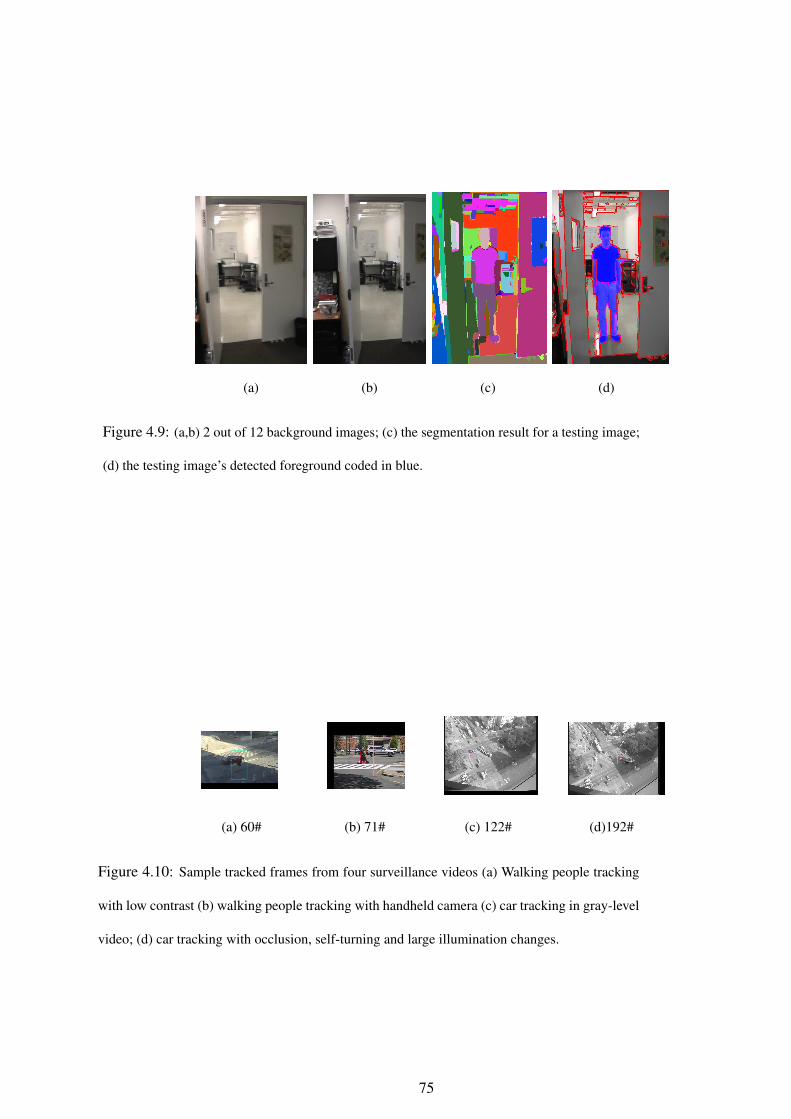
(a) (b) (c) (d)

Figure 4.9: (a,b) 2 out of 12 background images; (c) the segmentation result for a testing image;

(d) the testing image’s detected foreground coded in blue.

(a) 60# (b) 71# (c) 122# (d)192#

Figure 4.10: Sample tracked frames from four surveillance videos (a) Walking people tracking

with low contrast (b) walking people tracking with handheld camera (c) car tracking in gray-level

video; (d) car tracking with occlusion, self-turning and large illumination changes.

75

Chapter 5

Future Work

5.1 Future Work on Scene Recognition

5.1.1 Linear and Nonlinear Discriminative Learning [84, 87, 69, 100, 168, 113, 132]

Learning a discriminative projection of data categories (such as image patches sampled from different mate-

rial classes) is a general and important machine learning issue for classification problem. The discriminative

projection reduces the data dimensionality and more importantly increases the separating margins between

different data distributions. Fisher/Linear Discriminant Analysis (LDA) is the most popular algorithm which

provides the optimal projection of discriminative feature extraction under the assumption that the distribu-

tion of data samples from each category is a Gaussian function with equal prior and covariance matrix [165].

This strict condition on the optimal projection assumption largely limits its application on real computer vi-

sion tasks, as many visual data distributions are believed to be highly non-linear and non-Gaussian.

As a non-linear extension of LDA, Non-parametric discriminative analysis (NDA) [87] is proposed and

improved [69] for classification problems to overcome the Gaussian distribution constraint. The algorithm

only involves computing covariances from local neighbors and the global distribution can have an arbitrary

shape. Another important advantage of NDA is that the projected discriminative subspace is not limited to

be equal or less than (c−1) where c is the number of data classes. This property is very important to extract

statistically sufficient features with large enough dimensions when c is too small. However NDA has an

76

extra requirement on finding the within-class and between-class nearest neighbor sets for each data, which

can be very computationally expensive. To address this problem, Locality-sensitive hashing (LSH) [89, 107]

provides a solution for efficient, approximate nearest neighbor searching with the bounded error tolerance

and computational load. LSH has been successfully used for information retrieval over large collections of

images and shapes [94, 93, 107]. The difficulty of employing LSH for NDA is that NDA requires finding

both the within-class and between-class neighbor sets for each data entity while it is not very straightforward

to integrate different data class labels into the hash function designing and coding in LSH. As shown in the

second part of this proposal, we present a fast approximate method to compute the within-class and between-

class nearest neighbor sets for data samples by using unsupervised data clustering. Hastie [100] describes

another nonlinear global dimension reduction method by combining only local dimension information which

has the similar computational complexity with NDA.

Kernel Fisher Discriminant Analysis (KFDA) [132] is another popular nonlinear discriminative learning

technique . KFDA is designed to solve Fisher’s linear discriminant in the induced kernel feature space,

which yields a nonlinear discriminant in input space. Many kernel functions (such as Gaussian, Polynomial,

Spline and so on) can be used to map data into kernel space with possibly infinite dimensions. KFDA

has been applied to many pattern classification problems, eg. digits recognition, face detection. The main

difficulty of directly employing KFDA into our image patch discriminative learning is that the large number

of training patch samples from all 20 material classes causes the computation of KFDA’s pairwise kernel

matrix intractable. Some sparse approximation techniques [120, 119] on kernel method should be considered

to address this problem in the future plan. Another possible drawback of KFDA is that kernel method

originally intends to unravel the problem of (0-1) binary classifications and it can be cumbersome when the

data class number c is too large.

Kosinov et al. presents a distance-based discriminant analysis (DDA) method using iterative majoriza-

tion technique [113]. It gives promising results on both binary and multiple-class image categorization

tasks. This method is also eligible being combined with kernel reproducing projection [143, 159] (Ker-

nel DDA) for better performance on modelling more complex visual data. Zhu and Hastie [168] recently

77

propose a generalized non-parametric feature extraction method based on maximization of likelihood ratio

(LR) which claims to overcome the Gaussian assumption of LDA. Yet, its numerical optimization process

involves gradients on several hundred parameters in high dimension, which makes impractical for real world

problems. The last noticeable technique on discriminative learning is called discriminative log-linear model

[111] whose parameters are learned using generalized iterative scaling method [77]. This model have been

tested on problems of artificial data classification [111] and image categorization [79], with a more appealing

performance than LDA.

In the future work, we plan to evaluate and compare the performances of LDA, NDA, KFDA, DDA and

KDDA for recognition purpose on our 20 class image patch database. Additionally, we are also interested

to explore whether the linear coefficients computed from LDA can be further optimized in term of the class-

separation criterion by using stochastic optimization methods, such as Monte Carlo Markov Chain [134].

5.1.2 (Hierarchical) Bayesian Learning [81]

Fei-fei and Perona propose a novel generative Bayesian hierarchical model to learn and recognize 13 natu-

ral scene categories using Latent Dirichlet Allocation [64]. This approach provides a principled method to

learning relevant intermediate representations of visual scene automatically and without supervision. The

most significant difference of this approach is that there is no need of requiring experts to annotate image

regions for training purpose, compared with previous work (including ours [11]) [114, 101, 116, 105, 148,

127, 151]. Latent Dirichlet Allocation [64] is originally designed to represent and learn text-document mod-

els. With the adaption to image analysis [81], the algorithm provides a principled probabilistic framework

for learning models of image features using codewords. It provides a learning hierarchy where feature-

level codewords can further construct intermediate-level themes and the image categorization process is

performed by integrating out all intermediate-level hidden variables in a Bayesian fashion. In general, pa-

rameter learning and inference for Latent Dirichlet Allocation model is not computationally tractable due

to parameter coupling, but can be achieved via Monte Carlo Markov Chain [64], Laplace approximation

or Variational approximation [81]. A very challenging photo database including 13 natural categories is

78

used to testify the proposed Bayesian hierarchical model, and a satisfactory categorization performance is

reported [81]. Additionally, this model is also shown to ”be able to group categories of images into a sen-

sible hierarchy, similar to what humans would do” [81]. Our plan is to evaluate this model using our photo

database [11] for recognition performance comparison. It will be very interesting to explore how much gain

this model can achieve with much heavier computations than our algorithm.

5.1.3 Generative-Discriminative Random Field (DRF) for Material-Class Image Segmenta-

tion [118, 116, 117, 155, 156, 101]

Our scene recognition algorithm [11] has been demonstrated to be robust for noisy local image patch match-

ings (towards the learned appearance models of 20 material classes) and need no requirement on segmenting

local image regions as well. However our approach is capable to generate the image patch-wise labels of

20 material classes, as shown in Figure 3.4. Note that it is a difficult task for explicitly segmenting image

regions according to each material class, due to the inherent image appearance ambiguity. For example, an

image patch of ”blue sky” can be visually indistinguishable from a water patch [116, 101], unless we can

leverage some contextual information into the classification process. The general technique on modelling

image spatial contextual interactions is Markov Random Field (MRF) [88, 122] which basically performs as

a discontinuity-preserving smoothing process to integrate local neighboring information for robust labelling.

The Simulated Annealing and Monte Carlo Markov Chain based MRF parameter learning/infernce methods

[88] is very computational demanding and time-consuming. Recently (Loopy) Belief Propagation [137, 85]

and (Max-flow/mini-cut) Graph-cut [112] has been demonstrated to be two standard fast MRF solvers in

[152] with good results. In this proposal, we employ loopy belief propagation algorithm [85] to re-estimate

the image patch’s likelihood probability according to each material class density model for better material

detection results (Figure 3.4). To make the smoothing process of local observation measurements adaptive

to the image contents themselves, data observations can be directly fused into either the pairwise potential

functions in belief propagation [11] or the pairwise interaction energy term in graph-cut [112]. In summary,

all standard Markov Random Field model is considered as a probabilistic generative model.

79

Material-class image segmentation problem is indeed a conditional classification task (ie. finding hidden

labels conditionally on image observations), while generative framework (eg. Markov Random Field) ex-

pends efforts on modelling the joint distribution of image observations and their semantic labels which can

be very computationally expensive or even intractable. On the contrary, discriminative framework models

the conditional posterior probability directly which can possibly result in a simpler solution. As noted in

[116, 117], ”a potential advantage of employing the discriminative approach is that the true underlying gen-

erative framework can be quite complex even though the class posterior is simple”. Recently, Discriminative

Random Field (DRF) is proposed by [116], for image patch labelling task, based on the idea of Conditional

Random Field (CRF) [118]. DRF and CRF are discriminative models that formulate the conditional distri-

bution over labels (as hidden variables) using discriminative classifiers. The most common classifier used

in [118, 116, 117] is the logistic regression classifier [165, 5]. Both the association potential and interaction

potential functions in DRF utilize the log-linear model over labels on site-wise or pairwise observations.

Because the evaluation of the partition function in DRF is NP-hard problem, the model parameters are

actually learned using various approximate techniques, eg. mean-field or pseudo-likelihood; and the infer-

ence process can be performed using Iterated Conditional Modes [63] (ICM), loopy belief propagation [85]

(for site-wise Maximum Posterior Marginal solution) or max-flow/min-cut [112] (for Maximum A Posterior

solution). For details, refer to [116, 117, 118, 122].

Some other researchers also propose variations of CRF type method for image labelling [101] and object

recognition [156, 155]. Particularly, He et al. [101] adopt a (product of experts) neural network framework

[102] to compute the product of the local neighboring distributions as a single distribution for conditional

labelling. The neural network parameters are learned from a set of annotated images using contrastive diver-

gence [102]. Instead of logistic regression or neural network, Torralba et al. [156, 155] describe the Boosted

Conditional Random Field model by applying real boosting [86, 74] method to learn the graph structure and

local evidence of a conditional random field [118] additively for contextual-level object detection.

In summary, DRF offers a much flexible way to model more complex interactions using a learned clas-

sification function in the field model, compared with MRF by merely taking a predefined prior over interac-

80

tions. DRF is trained from a set of supervised data so that it is more task-driven for good results. Another

advantage of DRF over MRF is that the underlying interactions can be formulated in many forms: pixel

to pixel, region to region, segment to segment, object part to object part [117]. It greatly enhances DRF’s

modelling capacity for diversely visual data. In this proposal, we plan to investigate a simplified version of

CRF for the material-class image segmentation problem. It involves representing images as a set of regularly

or randomly sampled image patches; learning discriminative model-association functions; learning discrim-

inative pairwise interaction/potential functions and using loopy or tree structured belief propagation over

looped or star-shape random graphs for integrated conditional inference. Note that the local random graph

structures needs to be learned [156] or simply searched [65] before any parameter learning or inference.

5.2 Future Work on Dynamic Foreground/Background Segmentation

5.2.1 Modeling Spatial Interactions Among Image Segments

In above, we propose to extract foreground/background image or video regions by classifying over indi-

vidual image segments produced by a general segmentor [82]. To use contextual constraints, the accuracy

of figure/ground segmentation can be improved by modelling image segment’s spatial interactions as well.

This problem is generally addressed by Markov random field (MRF) model [88, 122, 85, 112], Discrim-

inative/Conditional Random Field [116, 117, 118] or the boosting-additive method on logistic classifiers

[105, 86, 74].

For pairs of neighboring image segments under finer scales (eg. images shown in Figure 4.6), the

between-similarity measurement are usually defined on the low-level image observations, such as the match-

ing scores of their associated color or gradient histograms. On the other hand, the logistic regression function

or alternative probabilistic discriminative classifiers can be trained from the joint feature vectors of pairs of

spatially adjacent segments under coarser scales [116, 117], using a supervised approach. The pairwise joint

feature pattern is directly encoded by learning the parameters of classifier functions1. In the future, we plan1For larger scaled indoor and outdoor images, many neighboring image segments of foreground or background are visually

dissimilar. Thus the interactions based on image similarity will model the labelling process of image segments very independently.

81

to investigate how to define the similarity measurement of a larger clique of image segments (ie. beyond

pairwise interactions).

Classification on hypotheses of constellations of image segments for labelling stability is the key contex-

tual learning/inference issue. Firstly, within Markov Random Field representation, segment-model appear-

ance matching responses are stated as data-model association energy terms and segment’s pairwise similar-

ities as neighboring interaction energy terms2. The figure/ground segmentation problem is then formulated

as a binary partitioning of a graph of nodes (ie. image segments), which can be solved using the max-

flow/mini-cut graph-cut techniques [112, 67] for Maximum A Posterior solution or (loopy) Belief Propaga-

tion [137, 85] for site-wise Maximum Posterior Marginal solution. Secondly, Discriminative/Conditional

Random Field [116, 117, 118] employs different classifiers to model the association and interaction energy

terms. A collections of discriminative classifiers (which can be defined separately) and their spatial inter-

actions largely increase the modelling capacity and flexibility of possible energy formulations. Classifiers

are discriminatively trained from a set of annotated data, which can make task-oriented image recognition

tasks with possibly more prevailing performance than general-purpose generative models (such as MRF

with general prior setting). Thirdly, [105] has shown that hypotheses for constellations of image segments

can be directly evaluated through using additive-boosting algorithms [86, 74] to measure the constellation’s

intrinsic content coherence under the same semantic meaning. A large collection of images have shown

being successfully interpreted as regions of horizontal ground, up-frontal man-made structure and sky in

[105].

5.2.2 Boundary-Preserving Image Segmentation

In this part of proposal, experiments are performed by using a general-purpose image segmentor [82]. By

adjusting the segmentor’s smoothing convolution kernel, scaling parameters and the minimal segmentation

size, we expect that images are moderately over-segmented and all the object-level boundaries can be pre-

In this case, logistic regression function can work on the joint feature space to learn the joint contextual pattern directly, regardless

that the spatial image segment neighbors are visually similar or dissimilar.2Especially, we borrow the energy term names from Graph-cut framework [112].

82

served for further processing (as described in [?]). The image segmentation method used in [82] is a graph

based partitioning algorithm based on local image color-texture observations. Because it is designed for

general purposes, object-level boundaries can not always be detected, especially for image sequences cap-

tured under severe appearance changing and illumination conditions. Parts of foreground and background

regions can group into a single partition due to their local homogeneity under strong shadow and motion

blur. To enhence the performance of boundary-preserving image segmentation, we propose to generate new

segmentation boundaries by thresholding belief maps (ie. the matching distance/density maps in Figure

4.5) produced by the learned foreground/background appearance models [148, 117]. It can be considered

as a specified image segmentor3 by using the domain knowledge directly. It can help detect object-level

boundaries based on the high-level multi-modal4 appearance model. Similarly, foreground/background’s

probability spatial prior maps based on kernel density evaluation in video sequences can also be treated as

belief maps on finding object-level boundaries by using the shape constraint.

5.2.3 Uncertainty Measurement and Random Graph Belief Propagation

Though image boundaries detection can be enhanced by employing both the general-purposed image seg-

mentors [82, 147] and domain-oriented belief maps thresholding [148, 117], there is no theoretical guarantee

that all desirable object-level boundaries can be preserved during above processes. In order to address this

problem, we plan to measure the confidence or uncertainty of decision making over individual image seg-

ments (ie. classifying image segments into foreground or background classes). One simple possibility is

that the uncertainty value can be obtained from the variance of matching scores from image patches within

each segment towards the foreground/background appearance models. For instance, if all image patches

have very similar matching responses given a specific appearance model, the decision making process is

considered to be very confident. Otherwise, if there are a lot contradict matching scores, the aggregated

classification process over the whole image segment should be much less confident.3It is equivalent to run a general-purpose image segmentor on real-valued belief maps.4The multi-modal appearance model can possibly convert nonhomogeneous image regions into homogeneous belief maps,

which make it more convenient for the specific task-driven segmentation.

83

Based on uncertainty measurements of image segments, we plan to develop a heuristic to find segment

candidates with suspicious (possibly incorrect) foreground/background labels. For each of those candidates,

we will not label it as a single unit, but rather label all individual image patches within the segment instead.

We further plan to formulate the patch labelling process using a Markov random field or conditional random

field representation by leveraging contextual constraints. A brief introduction on parameter learning and

inference algorithms on MRF or DRF is formerly described in section 5.1. Because we usually need to label

hundreds of patches inside suspicious image segments, the computational efficiency turns out to be the key

issue. Due to this reason, we propose to assemble each image patch with its spatial neighbors (and temporal

neighbors from contiguous frames in video) and simplify the graph topology of field model to be ”star-

shaped”, which can be efficiently learned and inferred using tree-structure belief propagation [137, 65].

The potential functions of messages in belief propagation can be defined according to the principles of

MRF or DRF (section 5.1) respectively.

In summary, images segments with high confidences will be labelled as foreground/background directly

(using the simple aggregation process described in section 4.4), while image segments with low confidences

will be marked as ”suspicious candidates” for further patch-wise labelling. This is an adaptive classification

strategy by first solving easier problems with less computations, and then harder problems containing more

ambiguities using more computations (as shown in above).

5.2.4 Parametric or Non-parametric Density base Appearance Model

In section 4.5, we compare the classification performances of object-level image mapping for eight algo-

rithms. Based on this comparison, we adopt Kernel based density estimator (KDE) [106] to construct the

nonparametric appearance density functions for foreground/background segmentation in videos, because of

KDE’s representative flexibility and computational efficiency [106]. In future work, we can use clustering

methods [5, 165] condensing the number of representative data samples in Kernel density estimator [106],

to further improve the computational speed. Note that the model selection problem of clustering techniques

is not very critical in our case, though there is no general good solution for that. Here we mainly concern

84

the trade-off between the density approximation accuracy of KDE towards the true density functions and the

computation gain obtained by condensing the number of kernels in KDE. The clustering model complexity

can be conservatively larger than the number of modes of the underlying multi-modal density functions. We

plan to investigate this issue in future work.

Because we represent any given image as a chuck of sampled image patches [?], it is equivalent to

represent a single huge dimensional data item by using a distribution of data samples with much lower di-

mensions. This representation can offer the modelling flexibility on controlling the rigidity on how much

or different new data can be integrated into the model when considering the temporal model updating pro-

cess from videos. For example, for the dynamic foreground appearance model, we expect that there is

no significant model shifting from one frame to its successive frame in a video sequence. If some new

”foreground-labelled” image patch samples from the next frame is visually very different5 with respect to

the current model, they have more chance to be outliers. If we assume that the background appearances can

be freely changing consequently, there will be no ”outlier-rejection” process for background. This heuris-

tic can be formulated into the sample’s surviving probability during resampling. More apparently different

patch samples has lower probability to survive through resampling; and vice versa. Further more, this

”model integrating with rejection” strategy should be designed to be adaptive with the changing behavior of

image contents in videos. Fast changing videos allow more difference tolerance, and slow changing videos

allow less difference tolerance in the temporal appearance model updating process6.

5.2.5 Automatic Key-Frame Selection for Interactive Foreground/Background Segmenta-

tion

In video based foreground/background segmentation applications, we only label the first frame manually (or

using an automatic initialization procedure described in section 4.5), build an initial appearance model for5The difference intensity can be measured as the density value of a new patch sample in frame t evaluated by the density

functions up to frame t− 1. Higher density value means less different or more consistent, and vice versa.6A similar term in machine learning literatures is called ”learning rate” which is a tradeoff between biases towards the history

model or new contents.

85

foreground and background, then propagate this model into successive frames. For fast content changing

videos (for instance, Karsten.avi in section 4.5 needs to be relabelled when unseen background appears from

behind the walking person. Unexpected, severely appearance-changing organs come out very commonly

in surgical videos.), it is very normal that some formerly unseen image contents consequently appear as

parts of dynamic background. The temporal adaption of the appearance model rooting from the first video

frame may be insufficient to recover temporal fast image content changes. To address this problem, we

propose to automatically extract multiple key-frames from a given video sequence based on techniques of

pairwise image matching [92, 93, 94, 107, 89, 95, 141] and spectral/graph partitioning [135, 136]. Note

that we define ”key-frames” as image frames containing mutually distinct visual contents and (probably)

representing modes in the whole video appearance model. Therefore we expect the video key-frames to

be automatically extracted containing significantly more amounts of appearance contents than just the first

frame. This can help the initial appearance model trained from multiple key-frames be more representative

and propagate more effectively in the temporal domain.

Particularly, we purpose to employ the pyramid match kernel approach [92] (which is based on the ideas

of multi-resolution histogram pyramid for recognition [95] and positive-definite kernel [145]) to efficiently

and effectively compute the matching scores of any given pair of image frames by matching two distributions

from sets of sampled image patches. The other two related image matching techniques are locality-sensitive

hashing [107, 89] and Earth Mover’s Distance [141, 93, 94]. After obtaining the matching scores for all

image frame pairs in video, we can either form them into the pairwise Affinity matrix and perform the

spectral clustering [135] to find modes of clusters as key-frames, or convert them as a weighted graph model

and execute the graph partitioning algorithm [136] to select key-frames. For these automatically extracted

key-frames, we plan to assign foreground/background labels onto their manually selected image regions by

using a publicly available image annotation tool: ”Label Me” [157], for the initial foreground/background

appearance model construction.

86

Chapter 6

Appendices

6.1 Appendix 1: Grey Level Cooccurrence Matrices: GLCM

Let us denote GLCM a N × N matrix Pi,j where N is the quantized level of pixel intensity and i, j =

0, 1, ..., N − 1. The diagonal elements (i = j) all represent pixel pairs with no grey level difference;

while the off-diagonal cells (i 6= j) represent pixel pairs with dissimilarity |i − j| increasing linearly

away from the diagonal. Therefore we have dissimilarity =∑N−1

i,j=1 (P (i, j)× |i− j|). Furthermore

ASM =∑N−1

i,j=1 P (i, j)2 measures the uniformity of the distribution of GLCM. µi =∑N−1

i,j=1 (P (i, j)× i|)

and µj =∑N−1

i,j=1 (P (i, j)× j|) are the means of the reference pixels or neighbor pixels. Similarly,

σi =√∑N−1

i,j=1 (P (i, j)× (i− µi)2) and σj =√∑N−1

i,j=1 (P (i, j)× (j − µj)2) are the respective stan-

dard deviations, and correlation =∑N−1

i,j=1 (P (i, j)× (i− µi)(j − µj))/(σi × σj). If the above means

and standard deviations are calculated from symmetrical GLCM, µ = µi = µj and σ = σi = σj . Finally

the output of 5 Haralick features are dissimilarity,ASM, µ, σ, correlation for each GLCM 1.

1Note that we choose the pair of reference and neighbor pixels according to 4 directions (45 degree each) and 1 or 2 pixel offsets.

Therefore we have 8 GLCMs for any image patch which results in a 40 component feature vector.

87

6.2 Appendix 2: Linear Discriminant Analysis: LDA

The following objective function

J(ω) =ωT SBω

ωT SW ω(6.1)

is maximized by solving a generalized eigenvector equation

SBω = λSW ω (6.2)

where

SW =1M

C∑

i=1

M∑

j=1

zij(Xj −mi)(Xj −mi)T (6.3)

SB =C∑

i=1

Mi

M(mi −m)(mi −m)T (6.4)

Denote that SB and SW are respectively named the between-class or within-class scatter matrix, xj is a

feature vector, mi is the mean of class i and m is the global mean of the data X , i = 1...C is a class number

(C is the total number of classes) and the binary membership function

zij =

1, if xj ∈ class i

0, otherwise

(6.5)

The LDA algorithm firstly perform the singular value decomposition (SVD) of SW

SW = UΛUT (6.6)

then transform SB into

S′B = Λ−

12 UT SBUΛ−

12 (6.7)

and compute the eigenvectors of

S′BV = VΛ (6.8)

where Λ is the diagonal matrix of eigenvalues of S′B . The optimal feature vectors Z are therefore

Z = AT X (6.9)

through the projected transform AT = VT Λ−12 UT . For dimension reduction, only the subset of eigenvectors

V and U with large eigenvalues are used in the transform. The dimension of the LDA projected subspace is

at most C − 1.

88

6.3 Appendix 3: Discriminative-GMM Algorithm

Linear Discriminant Analysis (LDA) is proposed to maximize the following objective function

J(ω) =ωTSBω

ωTSWω(6.10)

by solving a generalized eigenvector equation

SBω = λSWω (6.11)

where

SW =1M

N∑

i=1

M∑

j=1

zij(xj −mi)(xj −mi)T (6.12)

SB =N∑

i=1

Mi

M(mi −m)(mi −m)T (6.13)

Denote that SB and SW are respectively named the between-class or within-class scatter matrix, xj is a

feature vector, mi is the mean of class i and m is the global mean of the data X , i = 1...C is a class number

and the binary membership function

Lij =

1, if xj ∈ class i

0, otherwise

(6.14)

The LDA algorithm firstly perform the singular value decomposition (SVD) of SW

SW = UΛUT (6.15)

then transform SB into

S ′B = Λ−12 UTSBUΛ−

12 (6.16)

and compute the eigenvectors of

S ′BV = VΛ (6.17)

where Λ is the diagonal matrix of eigenvalues of S ′B. The optimal feature vectors Z are therefore

Z = ATX (6.18)

89

through the projected transform

AT = VT Λ−12 UT

For dimension reduction, only the subset of eigenvectors V and U with larger eigenvalues are used in the

transform. The dimension of the LDA projected subspace is at most C − 1.

After the projected data Z is obtained, GMM parameters π, µ,Σ are initialized as follows

µi =M∑

j=1

Lijxj , i = 1, 2, ...,N (6.19)

and πi = 1/N , Σi is a D dimensional identical matrix where i = 1, 2, ...,N . From the initial estimates,

π, µ,Σ are then re-estimated iteratively in an Expectation-Maximization [40] fashion. In the E-step,

Wij = πiP (zj ; µi, Σi) (6.20)

where Wij is the membership function of xj with class i and is normalized by

Wij =Wij∑

i=1,...,N Wij(6.21)

to satisfy the constraint∑

i=1,...,N Wij = 1. In the M-step, parameters π, µ,Σ are computed for each

mixture density function as follows

πi =1M

∑

j=1,...,M

Wij (6.22)

µi =

∑j=1,...,M Wijzj∑j=1,...,M Wij

(6.23)

Σi =

∑j=1,...,M Wij(zj − µi)(zj − µi)T

∑j=1,...,M Wij

(6.24)

When the EM algorithm converges (normally after 10 iteration in our case), we can update the within-

class and between-class scatter matrices SW ,SB from the membership function W estimated in GMM. The

updated SW ,SB improve the performance of LDA to find more discriminative projections.

SW =1M

N∑

i=1

M∑

j=1

Wij(xj −mi)(xj −mi)T (6.25)

SB =N∑

i=1

πi(mi −m)(mi −m)T (6.26)

90

where mi is the mean of class i, m is the mean of all the data.

mi =

∑j=1,...,M Wijxj∑

j=1,...,M Wij(6.27)

m =1M

∑

j=1,...,M

xj (6.28)

As a summary, our algorithm contains 2 loops of iterations. The outer loop is the LDA-GMM iterations

through the update of SW ,SB by W; the inner loop is the EM iterations of GMM. In section 3.5, the

convergency of discriminative-GMM algorithm is validated experimentally in terms of the increasing log-

likelihood of the fitness of the model and data

LL =M∑

j=1

N∑

i=1

log (πiP (zj ; µi,Σi)) (6.29)

and the decreasing ratios of the incorrectly clustered data under the fixed model complexity.

91

Bibliography

[1] Christopher M. Bishop, Neural Networks for Pattern Recognition, Oxford University Press, Oxford,

UK, 1995.

[2] Christopher M. Bishop, Pattern Recognition and Machine Learning, Springer-Verlag, New York, USA,

2006.

[3] G. Boccignone, Foveated Shot Detection for Video Segmentation, IEEE Transactions on Circuits and

Systems for Video Technology, 15:3, pp. 365-377, 2005.

[4] C. Mario Christoudias and Trevor Darrell, On Modelling Nonlinear Shape-and-Texture Appearance

Manifolds, Proceedings IEEE Conf. on Computer Vision and Pattern Recognition, 2005.

[5] R. Duda, P. Hart and D. Stork, Pattern classification. Wiley, New York. 2nd edition, (2000).

[6] A. Hanjalic, Shot-boundary detection: unraveled and resolved? IEEE Transactions on Circuits and

Systems for Video Technology, 12:2, pp. 90105, 2002.

[7] T. Hastie, R. Tibshirani and J. Friedman, The Elements of Statistical Learning: Data Mining, Inference

and Prediction, Springer-Verlag, New York, USA, 2001.

[8] J. Ho, M.-H. Yang, J. Lim, K.-C. Lee and D. Kriegman, Clustering apperances of objects under varying

illumination conditions. IEEE Conference on Computer Vision and Pattern Recognition (pp. 11–18),

2003.

92

[9] Le Lu, Gregory D. Hager and Laurent Younes, A Three Tiered Approach for Articulated Object Action

Modeling and Recognition, Neural Information Processing and System, Vancouver, B.C. Canada, Dec.

2004.

[10] Le Lu, Xiangtian Dai and Gregory D. Hager, A Particle Filter without Dynamics for Robust 3D Face

Tracking, IEEE Workshop of Face Processing in Video with CVPR’2004, June 2004, Washington DC,

USA.

[11] Le Lu, Kentaro Toyama and Gregory D. Hager, A Two Level Approach for Scene Recognition, IEEE

Computer Society Conference on Computer Vision and Pattern Recognition, June 2005, San Diego, USA.

[12] Le Lu and Rene Vidal, Combined Central and Subspace Clustering on Computer Vision Applications,

International Conference of Machine Learning, June 2006, Pittsburgh, USA.

[13] Le Lu and Gregory D. Hager, Dynamic Foreground-Background Extraction from Images and Videos

using Random Patches, Neural Information Processing and System, Vancouver, B.C. Canada, Dec. 2006.

[14] Le Lu, Xiangtian Dai and Gregory D. Hager, Efficient Particle Filtering Using RANSAC with Appli-

cation to 3D Face Tracking, International Journal of Image and Vision Computing, June 2006.

[15] Le Lu and Gregory D. Hager, A Nonparametric Treatment Unifying Dynamic Far-field and Close-field

Tracking, Submitted to IEEE Computer Society Conference on Computer Vision and Pattern Recognition,

June 2007.

[16] M. Osian and Luc Van Gool, Video Shot Characterization, Machine Vision and Application, 15:172-

177, 2004.

[17] S. Porter, M. Mirmehdi and B. Thomas, Temporal Video Segmentation and Classification of Edit

Effects, International Journal of Image and Vision Computing, pp. 1097-1106, 2003.

[18] C.E. Rasmussen and Chris Williams, Gaussian Processes for Machine Learning, MIT press, 2006.

[19] Bernhard Scholkopf and Alexander J. Smola, Learning with Kernels: Support Vector Machines, Reg-

ularization, Optimization and Beyond, Springer-Verlag, New York, USA, 2002.

93

[20] N. Sebe, M. Lew and A. Smeulders, Special Issues on Video Retrieval and Summarization, Computer

Vision and Image Understanding, Sept. 2003.

[21] John Shawe-Taylor and Nello Christianini, Kernel Methods for Pattern Analysis, Cambridge Univer-

sity Press, 2004.

[22] C. Stauffer and W. Grimson, Learning Patterns of Activity using Real-time Tracking, IEEE Trans.

Pattern Analysis and Machine Intelligence, Oct. 2000.

[23] M. Tipping and C. Bishop, Mixtures of probabilistic principal component analyzers. Neural Compu-

tation, 11, 443–482, (1999).

[24] R. Vidal and Y. Ma, A unified algebraic approach to 2-D and 3-D motion segmentation. European

Conference on Computer Vision (pp. 1–15), 2004.

[25] R. Vidal, Y. Ma, and S. Sastry, Generalized Principal Component Analysis (GPCA). IEEE Trans. on

Pattern Analysis and Machine Intelligence, 27, 1–15, (2005).

[26] V.N. Vapnik, The Nature of Statistical Learning Theory, Springer-Verlag, New York, USA, 2001.

[27] N. Vasconcelos and A. Lippman, Statistical Models of Video Structure for Content Analysis and

Characterization, IEEE Trans. on Image Processing, vol. 9, pp. 3-19, Jan. 2000.

[28] A.R. Webb, Statistical Pattern Recognition, John Wiley and Sons, 2002.

[29] K. Q. Weinberger and L. K. Saul, Unsupervised learning of image manifolds by semidefinite program-

ming. IEEE Conference on Computer Vision and Pattern Recognition (pp. 988–995), 2004.

[30] Y. Zhai and M. Shah, Video Scene Segmentation using Markov chain Monte Carlo, IEEE Trans. on

Multimedia, vol. 8, No. 4, pp. 686-697, August 2006.

[31] H. Zhang, A. Kankanhalli and S.W. Smoliar, Automatic Partitioning of Full-motion Video, Multimedia

System, vol 1, pp. 10-28, 1993.

94

[32] R. Zabih, J. Miller and K. Mai, A Feature based Algorithm for Detecting Cuts and Clssifying Scene

Breaks, Proc. of ACM multimedia, San Francisco, pp. 189-200, 1995.

[33] F. Aherne, N. Thacker, and P. Rockett, The Bhattacharyya Metric as an Absolute Similarity Measure

for Frequency Coded Data, Kybernetika, 34:4, pp. 363-68, 1998.

[34] V. Athitsos and S. Sclaroff, Estimating 3D Hand Pose From a Cluttered Image, CVPR, 2003.

[35] M. Brand, Shadow Puppetry, ICCV, 1999.

[36] R. Bowden and M. Sarhadi, A Non-linear of Shape and Motion for Tracking Finger Spelt American

Sign Language, Image and Vision Computing, 20:597-607, 2002.

[37] T. Cootes, G. Edwards and C. Taylor, Active Appearance Models, IEEE Trans. PAMI, 23:6, pp.

681-685, 2001.

[38] D. Cremers, T. Kohlberger and C. Schnrr, Shape statistics in Kernel Space for Variational Image

Segmentation, Pattern Recognition, 36:1929-1943, 2003.

[39] T. J. Darrell and A. P. Pentland, Recognition of Space-Time Gestures using a Distributed Representa-

tion, MIT Media Laboratory Vision and Modeling TR-197.

[40] A. Dempster, N. Laird and D. Rubin, Maximum likelihood from incomplete data via the EM algorithm,

Journal of the Royal Statistical Society, Series B, 39:1-38, 1977.

[41] A. Efros, A. Berg, G. Mori and J. Malik, Recognizing Action at a Distance. ICCV, pp. 726–733, 2003.

[42] W. T. Freeman and E. H. Adelson, The Design and Use of Steerable Filters, IEEE Trans. PAMI, 13:9,

pp. 891-906, 1991.

CVPR’94.

[43] T. Hastie and R. Tibshirani, Discriminant Analysis by Gaussian Mixtures. Journal of Royal Statistical

Society Series B, 58(1):155-176.

95

[44] W. Hawkins, P. Leichner and N. Yang, The Circular Harmonic Transform for SPECT Reconstruction

and Boundary Conditions on the Fourier Transform of the Sinogram, IEEE Trans. on Medical Imaging,

7:2, 1988.

[45] A. Heap and D. Hogg, Wormholes in Shape Space: Tracking through Discontinuous Changes in Shape,

ICCV, 1998.

[46] M. K. Hu, Visual pattern recognition by moment invariants, IEEE Trans. Inform. Theory, 8:179-187,

1962.

[47] B. Jedynak, H. Zheng and M. Daoudi, Statistical Models for Skin Detection, CVPR’03.

[48] M. J. Jones and J. M. Rehg, Statistical Color Models with Application to Skin Detection Int. J. of

Computer Vision, 46:1 pp: 81-96, 2002.

[49] B. Julesz, Textons, the elements of texture perception, and their interactions. Nature, 290:91-97, 1981.

[50] T. Leung and J. Malik, Representing and Recognizing the Visual Appearance of Materials using

Three-dimensional Textons, Int. Journal of Computer Vision, 41:1, pp. 29-44, 2001.

[51] M. Maila and J. Shi, Learning Segmentation with Random Walk, NIPS 2001.

[52] B. Moghaddam and A. Pentland, Probabilistic Visual Learning for Object Representation, IEEE

Trans. PAMI 19:7, 1997.

[53] A. Ng, M. Jordan and Y. Weiss, On Spectral Clustering: Analysis and an algorithm, NIPS, 2001.

[54] S. Satoh, Generalized Histogram: Empirical Optimization of Low Dimensional Features for Image

Matching, ECCV, 2004.

[55] J. Shi and J. Malik, Normalized Cuts and Image Segmentation, IEEE Trans. on PAMI, 2000.

[56] B. Stenger, A. Thayananthan, P. H. S. Torr, and R. Cipolla, Filtering Using a Tree-Based Estimator,

ICCV, II:1063-1070, 2003.

96

[57] C. Tomasi, S. Petrov and A. Sastry, 3D tracking = classification + interpolation, ICCV, 2003.

[58] R. Vidal and R. Hartley, Motion Segmentation with Missing Data using PowerFactorization and

GPCA, CVPR, 2004.

[59] Y. Weiss, Segmentation using eigenvectors: A Unifying view. ICCV, 1999.

[60] Lihi Zelnik-Manor and Michal Irani, Event-based video analysis, CVPR, 2001.

[61] S. Aksoy and R. Haralick, Feature Normalization and Likelihood-Based Similarity Measures for Image

Retrieval, Pattern Recognition Letters, 22(5):563-582, 2001.

[62] P. Anandan, A computational framework and an algorithm for the measurement of visual motion, Int.

Journal of Computer Vision, 1989.

[63] Besag, J., On the statistical analysis of dirty pictures (with discussions), Journal of the Royal Statistical

Society, Series B, 48:259–302.

[64] D. Blei, A. Ng and M. Jordan, Latent dirichlet allocation, Journal of Machine Learning Research,

3:993-1022, 2003.

[65] O. Boiman and M. Irani, Detecting Irregularities in Images and in Video, Int. Conf. on Computer

Vision, pp. 462-469, 2005.

[66] M. Boutell, J. Luo and C. Brown, Learning spatial configuration models using modified Dirichlet

priors, Workshop on Statistical Relational Learning, 2004.

[67] Y. Boykov and M. Jolly, Interactive Graph Cuts for Optimal boundary and Region Segmentation of

Objects in n-d Images, ICCV, 2001.

[68] L. Breiman, Bagging Predictors, Machine Learning, 24(2):123-140, 1996.

[69] M. Bressan and J. Vitria, Nonparametric discriminative analysis and nearest neighbor classification,

Pattern Recognition Letter, 2003.

97

[70] M. Brown and D.G. Lowe, Recognising Panoramas, Int. Conf. on Computer Vision , pp. 1218-1225,

Nice, France, 2003.

[71] Chih-Chung Chang and Chih-Jen Lin, LIBSVM: a library for support vector machines, 2001, Software

available at http://www.csie.ntu.edu.tw/ cjlin/libsvm.

[72] L. Chen, H. Liao, M. Ko, J. Lin, and G. Yu, A new LDA-based face recognition system which can

solve the small sample size problem, Journal of Pattern Recognition, 33(10):1713-1726, 2000.

[73] Y.-Y. Chuang, B. Curless, D. Salesin and R. Szeliski, Bayesian Approach to Digital Matting, CVPR,

2001.

[74] M. Collins, R. Schapire, and Y. Singer,Logistic regression, adaboost and bregman distances, Machine

Learning, vol. 48, no. 1-3, 2002.

[75] J. Corso and G. Hager, Coherent Regions for Concise and Stable Image Description, CVPR, 2005.

[76] O. Cula and K. Dana, Compact representation of bidirectional texture functions, CVPR I:1041-1047,

2001.

[77] J.N. Darroch and D. Ratcliff, Generalized Iterative Scaling for Log-Linear Models, Annals of Mathe-

matical statistics, Vol. 43, no. 5, pp. 1470-1480, 1972.

[78] J. De Bonet, P. Viola, A non-parametric multi-scale statistical model for natural images, NIPS, 1997.

[79] T. Deselaers; D. Keysers and H. Ney, Discriminative training for object recognition using image

patches, Computer Vision and Pattern Recognition, 2005.

[80] A. Efros, T. Leung, Texture Synthesis by Non-parametric Sampling, ICCV, 1999.

[81] L. Fei-Fei and P. Perona, A Bayesian Hierarchical Model for Learning Natural Scene Categories, IEEE

CVPR, 2005.

[82] P. Felzenszwalb and D. Huttenlocher, Efficient Graph-Based Image Segmentation, Int. J. Comp. Vis.,

59(2), 2004.

98

[83] R. Fergus, P. Perona and A. Zisserman, Object class recognition by unsupervised scale-invariant

learning, CVPR, 2003.

[84] R.A. Fisher, The use of multiple measurements in taxonomic problems, Annals of Eugenics, 7:179-

188, 1936.

[85] B. Frey and D. J. C. Mackay, A revolution: Belief proapagation in graphs with cycles, Advances in

Neural Information Processing Systems, 1997.

[86] J. Friedman, T. Hastie, and R. Tibshirani, Additive logistic regression: a statistical view of boosting,

Annals of Statistics, vol. 28, no. 2, 2000.

[87] K. Fukunaga and J. Mantock, Nonparametric discriminative analysis, IEEE Trans. on PAMI, Nov.

1983.

[88] S. Geman and D. Geman, Stochastic relaxation, Gibbs distributions, and the Bayesian restoration of

images, IEEE Trans. PAMI, 6:721741, 1984.

[89] A Gionis, P Indyk and R Motwani, Similarity Search in High Dimensions via Hashing, 25th Int. Conf.

on Very Large Databases (VLDB), 1999.

[90] G. Golub and C. Van Loan, Matrix Computations, Johns Hopkins University Press, 1996.

[91] T. Gonzalez, Clustering to minimize the maximum intercluster distance, Theoretical Computer Sci-

ence, 38:293-306, 1985.

[92] K. Grauman and T. Darrell, The Pyramid Match Kernel: Discriminative Classification with Sets of

Image Features, In Proceedings of the IEEE International Conference on Computer Vision, Beijing,

China, October 2005.

[93] K. Grauman and T. Darrell Efficient Image Matching with Distributions of Local Invariant Features, In

Proceedings IEEE Conference on Computer Vision and Pattern Recognition, San Diego, CA, June 2005.

[94] K. Grauman and T. Darrell, Fast Contour Matching Using Approximate Earth Movers Distance., In

Proc. IEEE Conf. on Computer Vision and Pattern Recognition, Washington D.C., June 2004.

99

[95] E. Hadjidemetriou, M. Grossberg, and S. Nayar, Multiresolution Histograms and their Use for Recog-

nition, IEEE Trans. on Pattern Analysis and Machine Intelligence, 26(7):831847, July 2004.

[96] B. Han and L. Davis, On-Line Density-Based Appearance Modeling for Object Tracking, ICCV 2005.

[97] G.D. Hager and P. Belhumeur, Efficient Region Tracking With Parametric Models of Geometry and

Illumination, IEEE Trans. on Pattern Analysis and Machine Intelligence, 1998.

[98] R. Haralick, K. Shanmugam, and I. Dinstein, Texture features for image classification. IEEE Trans.

on System, Man and Cybernatic, 1973.

[99] C. Harris and M. Stephens, A combined corner and edge detector, Proc. Alvey Vision Conf., pp.

147-151, 1988.

[100] T. Hastie and R. Tibshirani, Discriminant Adaptive Nearest Neighbor Classification, IEEE Trans. On

Patttern Analysis and Machine Intelligence, 1998.

[101] X. He, R. Zemel and M. Carreira-Perpinan, Multiscale Conditional Random Fields for Image Label-

ing, CVPR, 2004.

[102] G. E. Hinton:, Training products of experts by minimizing contrastive divergence, Neural Computa-

tion, 14:17711800, 2002.

[103] T. K. Ho, The random subspace method for constructing decision forests, IEEE Trans. on PAMI,

20(8):832-844, 1998.

[104] Thomas Hofmann, Unsupervised Learning by Probabilistic Latent Semantic Analysis, Machine

Learning Journal, 42(1), pp.177-196, 2001.

[105] Derek Hoiem, Alexei A. Efros and Martial Hebert, Automatic Photo Pop-up, Proc. of SIGGRAPH,

2005.

[106] A. Ihler, Kernel Density Estimation Matlab Toolbox, http://ssg.mit.edu/ ihler/code/kde.shtml.

100

[107] P. Indyk and N. Thaper, Fast Image Retrieval via Embeddings, the3rd Int.l Workshop on Statistical

and Computational Theories of Vision, 2003.

[108] M. Irani, P. Anandan, and Meir Cohen, Direct Recovery of Planar-Parallax from Multiple Frames,

ICCV’99 Workshop: Vision Algorithms 99, Corfu, 1999.

[109] M. Irani and P. Anandan, About Direct Methods, ICCV’99 Workshop: Vision Algorithms 99, Corfu,

1999.

[110] T. Kadir and M. Brady, Scale, saliency and image description, IJCV, 45(2):83105, 2001.

[111] D. Keysers and H. Ney, Linear discriminant analysis and discriminative log-linear modeling, Int.

Cof. on Pattern Recognition, 2004.

[112] V. Kolmogorov and R. Zabih, What Energy Functions can be Minimized via Graph Cuts? IEEE

Trans. on PAMI, Feb. 2004.

[113] S. Kosinov, S. Marchand-Maillet and T. Pun, Visual object categorization using distance-based dis-

criminant analysis, In Proc. of the 4th Int. Workshop on Multimedia Data and Document Engineering,

Washington, DC, 2004.

[114] S. Kumar and M. Hebert, Man-made structure detection in natural images using a causal multiscale

random field, CVPR, 1:119-126, 2003.

[115] S. Kumar, A. C. Loui and M. Hebert, An Observation-Constrained Generative Approach for Proba-

bilistic Classification of Image Regions, Image and Vision Computing, 21:87-97, 2003.

[116] S. Kumar and M. Hebert, Discriminative Random Fields: A Discriminative Framework for Con-

textual Interaction in Classification, IEEE International Conference on Computer Vision (ICCV), 2003.

[117] S. Kumar and M. Hebert, A Hierarchical Field Framework for Unified Context-Based Classification,

IEEE International Conference on Computer Vision (ICCV), 2005.

101

[118] J. Lafferty, A. McCallum, and F. Pereira, Conditional random fields: Probabilistic models for seg-

menting and labeling sequence data, Int. Conf. of Machine Learning, pp. 282289, 2001.

[119] N. D. Lawrence, Gaussian process models for visualisation of high dimensional data, Advances in

Neural Information Processing Systems, MIT Press, Cambridge, MA, 2004.

[120] N. D. Lawrence, M. Seeger and R. Herbrich, Fast sparse Gaussian process methods: the informative

vector machine, Advances in Neural Information Processing Systems, MIT Press, Cambridge, MA, 2003.

[121] T. Leung and J. Malik, Representing and Recognizing the Visual Appearance of Materials using

Three-Dimensional Textons, Int. J. Comp. Vis.,43(1):29-44, 2001.

[122] S. Z. Li, Markov Random Field Modeling in Image Analysis, Springer-Verlag Tokyo, 2001.

[123] Y. Li, J. Sun, C.-K. Tang and H.-Y. Shum, Lazy Snapping, Proc. of SIGGRAPH, 2004.

[124] Y. Li, J. Sun and H.-Y. Shum. Video Object Cut and Paste, Proc. of SIGGRAPH, 2005.

[125] T. Lindeberg, Principles for automatic scale selection, Handbook on Computer Vision and Applica-

tions, 2:239–274, Academic Press, Boston, 1999.

[126] D. Lowe, Distinctive image features from scale-invariant keypoints, Int. J. Comp. Vis., 60(2):91-110,

2004.

[127] J. Luo, A. Singhal, S. Etz, and R. Gray, A computational approach to determination of main subject

regions in photographic images, Image Vision Computing, 22(3):227-241, 2004.

[128] J. Malik, S. Belongie, T. Leung and J. Shi, Contour and Texture Analysis for Image Segmentation,

Int. J. Comp. Vis., 43(1):7-27, 2001.

[129] D. Martin, C. Fowlkes, J. Malik, Learning to Detect Natural Image Boundaries Using Local Bright-

ness, Color, and Texture Cues, IEEE Trans. on PAMI, 26(5):530-549, May 2004.

[130] K. Mikolajczyk, C. Schmid, A performance evaluation of local descriptors, IEEE Transactions on

Pattern Analysis and Machine Intelligence, to appear.

102

[131] K. Mikolajczyk and C. Schmid, Scale and affine invariant interest point detectors, International

Journal of Computer Vision, Volume 60, Number 1, 2004.

[132] K.-R. Muller, S. Mika, G. Rtsch, K. Tsuda, and B. Schlkopf, An introduction to kernel-based learning

algorithms, IEEE Transactions on Neural Networks, 12(2):181-201, 2001.

[133] A. Mittal and N. Paragios, Motion-based Background Substraction using Adaptive Kernel Density

Estimation, CVPR, 2004.

[134] Radford M. Neal, Probabilistic Inference Using Markov Chain Monte Carlo Methods, University of

Toronto, 1993.

[135] A. Ng, M. Jordan and Y. Weiss, On Spectral Clustering: Analysis and an algorithm, NIPS, 2001.

[136] C. W. Ngo, Y. F. Ma and H. J. Zhang, Video Summarization and Scene Detection by Graph Modeling,

IEEE Trans on Circuits and Systems for Video Technology, vol. 15, no. 2, pp. 296-305, Feb 2005.

[137] J. Pearl, Probabilistic Reasoning in Intelligent Systems: Networks of Plausible Inference, Morgan

Kaufmann, 1988.

[138] X. Ren and J. Malik, Learning a classification model for segmentation, ICCV, 2003.

[139] C. Rother, V. Kolmogorov and A. Blake. Interactive Foreground Extraction using Iterated Graph

Cuts, Proc. of SIGGRAPH, 2004.

[140] F. Rothganger, S. Lazebnik, C. Schmid and J. Ponce, yes 3D object modeling and recognition using

affine-invariant patches and multi-view spatial constraints, In IEEE Conference on Computer Vision and

Pattern Recognition, June 2003.

[141] Y. Rubner, C. Tomasi, and L. Guibas, The Earth Movers Distance as a Metric for Image Retrieval,

International Journal of Computer Vision, 40(2):99121, 2000.

[142] C. Schmid, Weakly supervised learning of visual models and its application to content-based retrieval,

Int. Journal of Computer Vision, Volume 56, Number 1, 2004.

103

[143] B. Scholkopf and A. Smola, Learning with Kernels Support Vector Machines, Regularization, Opti-

mization and Beyond, MIT Press, Cambridge, MA, 2002.

[144] N. Serrano, A. Savakis and J. Luo, Improved scene classification using efficient low-level features

and semantic cues, Pattern Recognition 37(9):1773-1784, 2004.

[145] J. Shawe-Taylor and N. Cristianini, Kernel Methods for Pattern Analysis, Cambridge University

Press, 2004.

[146] Yaser Sheikh and Mubarak Shah, Bayesian Object Detection in Dynamic Scenes, CVPR, 2005.

[147] J. Shi and J. Malik, Normalized Cuts and Image Segmentation, IEEE Transactions on Pattern

Analysis and Machine Intelligence, 2000.

[148] A. Singhal, J. Luo and W. Zhu, Probabilistic Spatial Context Models for Scene Content Understand-

ing, CVPR, 2003.

[149] J. Sivic and A. Zisserman, Video Data Mining Using Configurations of Viewpoint Invariant Regions,

IEEE Conf. on Computer Vision and Pattern Recognition, 2004.

[150] J. Sivic and A. Zisserman, Video Google: A Text Retrieval Approach to Object Matching in Videos,

Int. Conf. on Computer Vision, 2003.

[151] M. Szummer and R. W. Picard, Indoor-outdoor image classification, IEEE Int. Workshop Content-

Based Access Image Video Databases, 1998.

[152] M. F. Tappen and W. T. Freeman, Comparison of graph cuts with belief propagation for stereo, using

identical MRF parameters, IEEE Intl. Conference on Computer Vision , Nice, France, 2003.

[153] Y.W. Teh, M.I. Jordan, M.J. Beal and D.M. Blei, Hierarchical Dirichlet Processes, Journal of Amer-

ican Statistical Association, in press, 2006.

[154] Philip H. S. Torr and A. Zisserman, Feature Based Methods for Structure and Motion Estimation,

ICCV’99 Workshop: Vision Algorithms 99, Corfu, 1999.

104

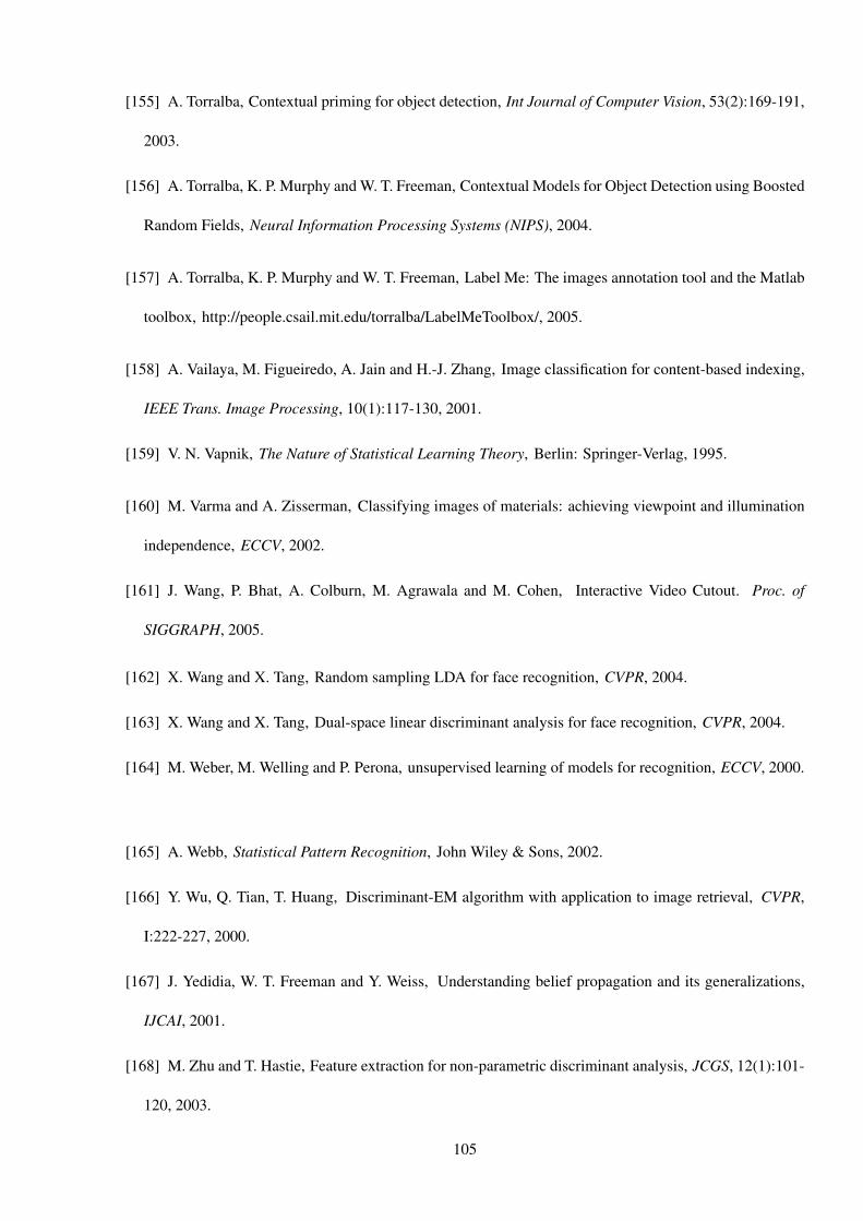
[155] A. Torralba, Contextual priming for object detection, Int Journal of Computer Vision, 53(2):169-191,

2003.

[156] A. Torralba, K. P. Murphy and W. T. Freeman, Contextual Models for Object Detection using Boosted

Random Fields, Neural Information Processing Systems (NIPS), 2004.

[157] A. Torralba, K. P. Murphy and W. T. Freeman, Label Me: The images annotation tool and the Matlab

toolbox, http://people.csail.mit.edu/torralba/LabelMeToolbox/, 2005.

[158] A. Vailaya, M. Figueiredo, A. Jain and H.-J. Zhang, Image classification for content-based indexing,

IEEE Trans. Image Processing, 10(1):117-130, 2001.

[159] V. N. Vapnik, The Nature of Statistical Learning Theory, Berlin: Springer-Verlag, 1995.

[160] M. Varma and A. Zisserman, Classifying images of materials: achieving viewpoint and illumination

independence, ECCV, 2002.

[161] J. Wang, P. Bhat, A. Colburn, M. Agrawala and M. Cohen, Interactive Video Cutout. Proc. of

SIGGRAPH, 2005.

[162] X. Wang and X. Tang, Random sampling LDA for face recognition, CVPR, 2004.

[163] X. Wang and X. Tang, Dual-space linear discriminant analysis for face recognition, CVPR, 2004.

[164] M. Weber, M. Welling and P. Perona, unsupervised learning of models for recognition, ECCV, 2000.

[165] A. Webb, Statistical Pattern Recognition, John Wiley & Sons, 2002.

[166] Y. Wu, Q. Tian, T. Huang, Discriminant-EM algorithm with application to image retrieval, CVPR,

I:222-227, 2000.

[167] J. Yedidia, W. T. Freeman and Y. Weiss, Understanding belief propagation and its generalizations,

IJCAI, 2001.

[168] M. Zhu and T. Hastie, Feature extraction for non-parametric discriminant analysis, JCGS, 12(1):101-

120, 2003.

105

[169] S.C. Zhu, Y.N. Wu, and D. Mumford, Minimax entropy principle and its applications to texture

modeling, Neural Computation, 9:1627-1660, 1997.

106