exploring data from the 1000 genomes project in ... · exploring data from the 1000 genomes project...

Exploring data from the 1000 Genomes project inBioconductor’s ind1KG package

VJ Carey

October 2, 2012

Contents

1 Overview 1

2 External data acquisition 22.1 Manual extraction of a multi-Mb chunk . . . . . . . . . . . . . . . . . . . 22.2 Programmatic extraction of annotated regions . . . . . . . . . . . . . . . 5

3 Exploring a samtools pileup 6

4 Checking samtools-based calls against other calls 84.1 HapMap Phase II calls . . . . . . . . . . . . . . . . . . . . . . . . . . . . 84.2 Affy SNP 6.0 chip calls . . . . . . . . . . . . . . . . . . . . . . . . . . . . 9

5 Relating possibly novel variants to existing annotation 105.1 Browser-based visualization . . . . . . . . . . . . . . . . . . . . . . . . . 105.2 Browser-based annotation extraction and comparison . . . . . . . . . . . 125.3 Exercises . . . . . . . . . . . . . . . . . . . . . . . . . . . . . . . . . . . . 17

1 Overview

In this document we will look at high-coverage NGS data obtained on NA19240, be-cause we have the HapMap phase II genotypes (4 mm SNP) for this individual inGGtools/hmyriB36, and we have an affy 6.0 SNP CEL file for this individual (andher cohort) as well.

There are three main objectives discussed in this document.

• We describe how data published in the 1000 genomes (1KG) project can be im-ported for investigations using R. This involves the use of the Rsamtools package.We provide serialized instances of various relevant data elements so that large ob-jects distributed from the project need not be redistributed for these illustrations.

1

• We describe how information on variants can be related to existing annotationusing rtracklayer to check for events in regulatory regions, for example.

• We discuss how information in the samtools ’pileup’ format can be checked froma statistical perspective to explore how ‘known’ variants in the sample compare tothe putatively newly discovered variants.

The reads examined in the document are all from the Illumina sequencing platform;additional work is sketched facilitating comparison with (released) read libraries basedon 454 or ABI platforms.

2 External data acquisition

2.1 Manual extraction of a multi-Mb chunk

We will focus on this individual’s chromosome 6. We acquired

NA19240.chrom6.SLX.maq.SRP000032.2009_07.bam

and the associated bai and bas files from

ftp://ftp-trace.ncbi.nih.gov/1000genomes/ftp/pilot_data/data/

NA19240/alignment/NA19240.chrom6.SLX.maq.SRP000032.2009_07.bam.bas

Note that it is possible to work with these files remotely in R, without moving them tothe local machine, thanks to the remote access facilities built in to samtools and exposedin R.

We use

samtools view \

NA19240.chrom6.SLX.maq.SRP000032.2009_07.bam |head -3000000 > na19240_3M.sam

to obtain a parsable text file, presumably of 3 million reads that aligned, using MAQ,nearest the 5’ end of the p arm of chr6. This is because we expect the bam file to besorted. We picked the number 3 million out of thin air.

This sam format file can be converted to bam format using the samtools importfacility. We took chromosome 6 reference sequence from

ftp://ftp-trace.ncbi.nih.gov/1000genomes/ftp/technical/

reference/human_b36_female.fa.gz

and indexed it and used

samtools import femchr6.fa.fai na19240_3M.sam na19240_3M.bam

2

to generate the bam file.We imported this into R using Bioconductor’s Rsamtools with a straight application

of scanBam. The result is saved in the package as n240.

> library(ind1KG)

> if (!exists("n240"))

+ data(n240)

This is a list of lists, and we check on the contents of the elements as follows:

> names(n240[[1]])

[1] "qname" "flag" "rname" "strand" "pos" "qwidth" "mapq" "cigar"

[9] "mrnm" "mpos" "isize" "seq" "qual"

We check the classes:

> sapply(n240[[1]], class)

qname flag rname strand pos

"character" "integer" "factor" "factor" "integer"

qwidth mapq cigar mrnm mpos

"integer" "integer" "character" "factor" "integer"

isize seq qual

"integer" "DNAStringSet" "PhredQuality"

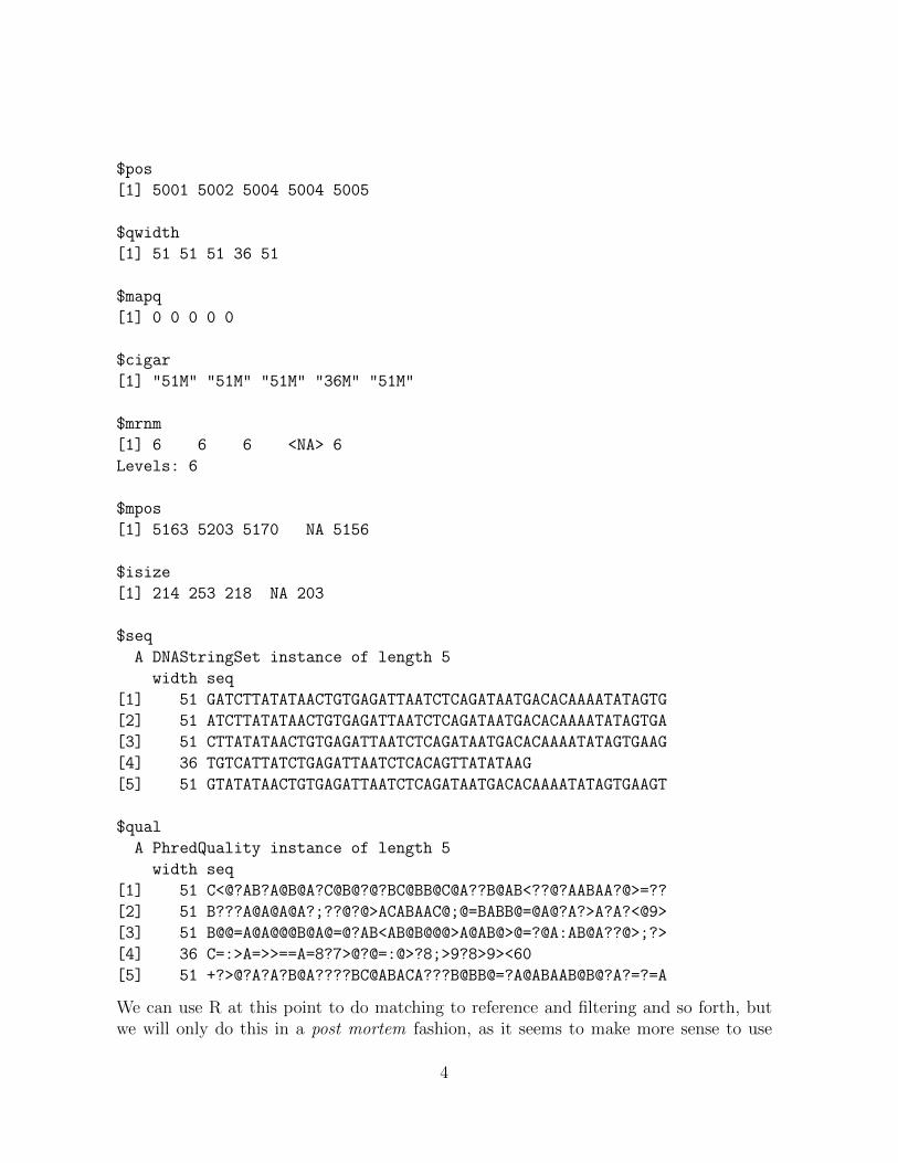
We get a small number of exemplars from each element:

> lapply(n240[[1]], head, 5)

$qname

[1] "EAS254_13:7:88:1639:15041" "EAS139_43:2:31:1128:9551"

[3] "EAS254_13:8:68:520:6861" "BGI-FC20AHFAAXX_6_26_477:352"

[5] "EAS139_43:6:71:1575:10961"

$flag

[1] 35 35 35 16 35

$rname

[1] 6 6 6 6 6

Levels: 6

$strand

[1] + + + - +

Levels: + - *

3

$pos

[1] 5001 5002 5004 5004 5005

$qwidth

[1] 51 51 51 36 51

$mapq

[1] 0 0 0 0 0

$cigar

[1] "51M" "51M" "51M" "36M" "51M"

$mrnm

[1] 6 6 6 <NA> 6

Levels: 6

$mpos

[1] 5163 5203 5170 NA 5156

$isize

[1] 214 253 218 NA 203

$seq

A DNAStringSet instance of length 5

width seq

[1] 51 GATCTTATATAACTGTGAGATTAATCTCAGATAATGACACAAAATATAGTG

[2] 51 ATCTTATATAACTGTGAGATTAATCTCAGATAATGACACAAAATATAGTGA

[3] 51 CTTATATAACTGTGAGATTAATCTCAGATAATGACACAAAATATAGTGAAG

[4] 36 TGTCATTATCTGAGATTAATCTCACAGTTATATAAG

[5] 51 GTATATAACTGTGAGATTAATCTCAGATAATGACACAAAATATAGTGAAGT

$qual

A PhredQuality instance of length 5

width seq

[1] 51 C<@?AB?A@B@A?C@B@?@?BC@BB@C@A??B@AB<??@?AABAA?@>=??

[2] 51 B???A@A@A@A?;??@?@>ACABAAC@;@=BABB@=@A@?A?>A?A?<@9>

[3] 51 B@@=A@A@@@B@A@=@?AB<AB@B@@@>A@AB@>@=?@A:AB@A??@>;?>

[4] 36 C=:>A=>>==A=8?7>@?@=:@>?8;>9?8>9><60

[5] 51 +?>@?A?A?B@A????BC@ABACA???B@BB@=?A@ABAAB@B@?A?=?=A

We can use R at this point to do matching to reference and filtering and so forth, butwe will only do this in a post mortem fashion, as it seems to make more sense to use

4

samtools directly to do, for example, SNP calling.

2.2 Programmatic extraction of annotated regions

(This code segment suggested by Martin Morgan.)We can use the GenomicFeatures package to obtain intervals defining various genomic

elements.

> library(GenomicFeatures)

> library(TxDb.Hsapiens.UCSC.hg18.knownGene)

> txdb = TxDb.Hsapiens.UCSC.hg18.knownGene

> txdb

TranscriptDb object:

| Db type: TranscriptDb

| Supporting package: GenomicFeatures

| Data source: UCSC

| Genome: hg18

| Genus and Species: Homo sapiens

| UCSC Table: knownGene

| Resource URL: http://genome.ucsc.edu/

| Type of Gene ID: Entrez Gene ID

| Full dataset: yes

| miRBase build ID: NA

| transcript_nrow: 66803

| exon_nrow: 266688

| cds_nrow: 221991

| Db created by: GenomicFeatures package from Bioconductor

| Creation time: 2012-09-10 12:55:02 -0700 (Mon, 10 Sep 2012)

| GenomicFeatures version at creation time: 1.9.39

| RSQLite version at creation time: 0.11.1

| DBSCHEMAVERSION: 1.0

The transcripts method will obtain ranges of transcripts with constraints.

> tx6 <- transcripts(txdb, vals = list(tx_chrom = "chr6"))

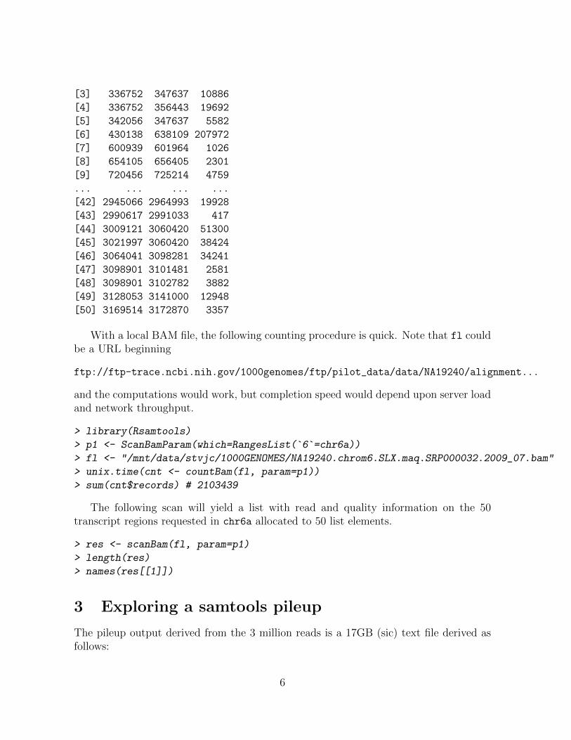
> chr6a <- head(unique(sort(ranges(tx6))), 50)

> chr6a

IRanges of length 50

start end width

[1] 237101 296355 59255

[2] 249628 296353 46726

5

[3] 336752 347637 10886

[4] 336752 356443 19692

[5] 342056 347637 5582

[6] 430138 638109 207972

[7] 600939 601964 1026

[8] 654105 656405 2301

[9] 720456 725214 4759

... ... ... ...

[42] 2945066 2964993 19928

[43] 2990617 2991033 417

[44] 3009121 3060420 51300

[45] 3021997 3060420 38424

[46] 3064041 3098281 34241

[47] 3098901 3101481 2581

[48] 3098901 3102782 3882

[49] 3128053 3141000 12948

[50] 3169514 3172870 3357

With a local BAM file, the following counting procedure is quick. Note that fl couldbe a URL beginning

ftp://ftp-trace.ncbi.nih.gov/1000genomes/ftp/pilot_data/data/NA19240/alignment...

and the computations would work, but completion speed would depend upon server loadand network throughput.

> library(Rsamtools)

> p1 <- ScanBamParam(which=RangesList(`6`=chr6a))> fl <- "/mnt/data/stvjc/1000GENOMES/NA19240.chrom6.SLX.maq.SRP000032.2009_07.bam"

> unix.time(cnt <- countBam(fl, param=p1))

> sum(cnt$records) # 2103439

The following scan will yield a list with read and quality information on the 50transcript regions requested in chr6a allocated to 50 list elements.

> res <- scanBam(fl, param=p1)

> length(res)

> names(res[[1]])

3 Exploring a samtools pileup

The pileup output derived from the 3 million reads is a 17GB (sic) text file derived asfollows:

6

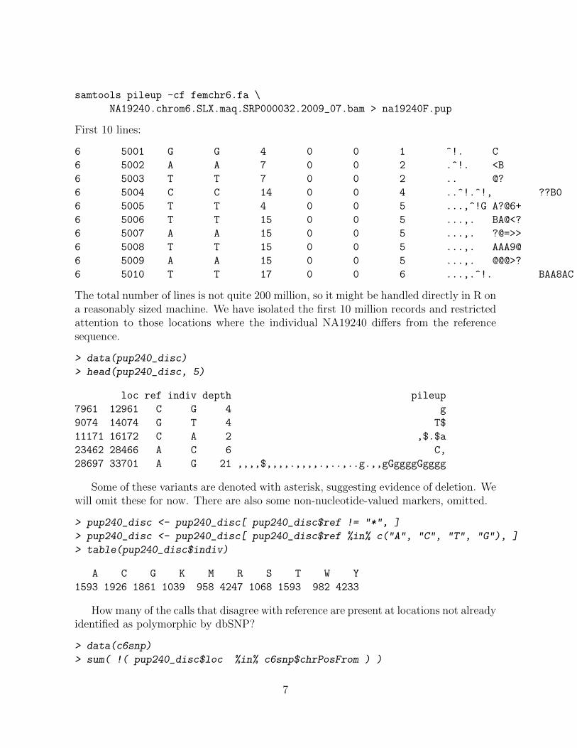
samtools pileup -cf femchr6.fa \

NA19240.chrom6.SLX.maq.SRP000032.2009_07.bam > na19240F.pup

First 10 lines:

6 5001 G G 4 0 0 1 ^!. C

6 5002 A A 7 0 0 2 .^!. <B

6 5003 T T 7 0 0 2 .. @?

6 5004 C C 14 0 0 4 ..^!.^!, ??B0

6 5005 T T 4 0 0 5 ...,^!G A?@6+

6 5006 T T 15 0 0 5 ...,. BA@<?

6 5007 A A 15 0 0 5 ...,. ?@=>>

6 5008 T T 15 0 0 5 ...,. AAA9@

6 5009 A A 15 0 0 5 ...,. @@@>?

6 5010 T T 17 0 0 6 ...,.^!. BAA8AC

The total number of lines is not quite 200 million, so it might be handled directly in R ona reasonably sized machine. We have isolated the first 10 million records and restrictedattention to those locations where the individual NA19240 differs from the referencesequence.

> data(pup240_disc)

> head(pup240_disc, 5)

loc ref indiv depth pileup

7961 12961 C G 4 g

9074 14074 G T 4 T$

11171 16172 C A 2 ,$.$a

23462 28466 A C 6 C,

28697 33701 A G 21 ,,,,$,,,,.,,,,.,..,..g.,,gGggggGgggg

Some of these variants are denoted with asterisk, suggesting evidence of deletion. Wewill omit these for now. There are also some non-nucleotide-valued markers, omitted.

> pup240_disc <- pup240_disc[ pup240_disc$ref != "*", ]

> pup240_disc <- pup240_disc[ pup240_disc$ref %in% c("A", "C", "T", "G"), ]

> table(pup240_disc$indiv)

A C G K M R S T W Y

1593 1926 1861 1039 958 4247 1068 1593 982 4233

How many of the calls that disagree with reference are present at locations not alreadyidentified as polymorphic by dbSNP?

> data(c6snp)

> sum( !( pup240_disc$loc %in% c6snp$chrPosFrom ) )

7

[1] 4075

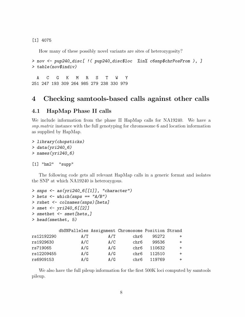
How many of these possibly novel variants are sites of heterozygosity?

> nov <- pup240_disc[ !( pup240_disc$loc %in% c6snp$chrPosFrom ), ]

> table(nov$indiv)

A C G K M R S T W Y

251 247 193 309 264 985 279 238 330 979

4 Checking samtools-based calls against other calls

4.1 HapMap Phase II calls

We include information from the phase II HapMap calls for NA19240. We have asnp.matrix instance with the full genotyping for chromosome 6 and location informationas supplied by HapMap.

> library(chopsticks)

> data(yri240_6)

> names(yri240_6)

[1] "hm2" "supp"

The following code gets all relevant HapMap calls in a generic format and isolatesthe SNP at which NA19240 is heterozygous.

> snps <- as(yri240_6[[1]], "character")

> hets <- which(snps == "A/B")

> rshet <- colnames(snps)[hets]

> smet <- yri240_6[[2]]

> smethet <- smet[hets,]

> head(smethet, 5)

dbSNPalleles Assignment Chromosome Position Strand

rs12192290 A/T A/T chr6 95272 +

rs1929630 A/C A/C chr6 99536 +

rs719065 A/G A/G chr6 110632 +

rs12209455 A/G A/G chr6 112510 +

rs6909153 A/G A/G chr6 119769 +

We also have the full pileup information for the first 500K loci computed by samtoolspileup.

8

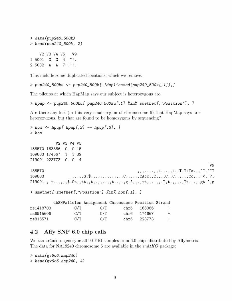
> data(pup240_500k)

> head(pup240_500k, 2)

V2 V3 V4 V5 V9

1 5001 G G 4 ^!.

2 5002 A A 7 .^!.

This include some duplicated locations, which we remove.

> pup240_500ku <- pup240_500k[ !duplicated(pup240_500k[,1]),]

The pileups at which HapMap says our subject is heterozygous are

> hpup <- pup240_500ku[ pup240_500ku[,1] %in% smethet[,"Position"], ]

Are there any loci (in this very small region of chromosome 6) that HapMap says areheterozygous, but that are found to be homozygous by sequencing?

> hom <- hpup[ hpup[,2] == hpup[,3], ]

> hom

V2 V3 V4 V5

158570 163386 C C 15

169883 174667 T T 89

219091 223773 C C 4

V9

158570 ,,,....,,t.,..,t..T.TtTa..,^~,^~T

169883 ..,,,$.$,,.,..,,...,..C,....,CAcc,,C,,,,C,.C..,..,Cc,..^<,^?,

219091 ,.t..,,,,$.Gt,,tt,,t,.,,..,,t..,.,g.A,,.,tt,,..,,.T,t.,,,.,Tt...,.gt.^,g

> smethet[ smethet[,"Position"] %in% hom[,1], ]

dbSNPalleles Assignment Chromosome Position Strand

rs1418703 C/T C/T chr6 163386 +

rs6915606 C/T C/T chr6 174667 +

rs815571 C/T C/T chr6 223773 +

4.2 Affy SNP 6.0 chip calls

We ran crlmm to genotype all 90 YRI samples from 6.0 chips distributed by Affymetrix.The data for NA19240 chromosome 6 are available in the ind1KG package:

> data(gw6c6.snp240)

> head(gw6c6.snp240, 4)

9

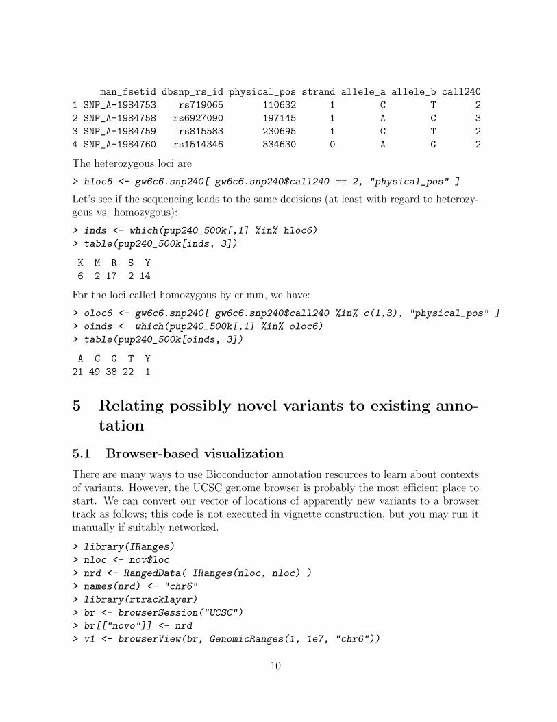
man_fsetid dbsnp_rs_id physical_pos strand allele_a allele_b call240

1 SNP_A-1984753 rs719065 110632 1 C T 2

2 SNP_A-1984758 rs6927090 197145 1 A C 3

3 SNP_A-1984759 rs815583 230695 1 C T 2

4 SNP_A-1984760 rs1514346 334630 0 A G 2

The heterozygous loci are

> hloc6 <- gw6c6.snp240[ gw6c6.snp240$call240 == 2, "physical_pos" ]

Let’s see if the sequencing leads to the same decisions (at least with regard to heterozy-gous vs. homozygous):

> inds <- which(pup240_500k[,1] %in% hloc6)

> table(pup240_500k[inds, 3])

K M R S Y

6 2 17 2 14

For the loci called homozygous by crlmm, we have:

> oloc6 <- gw6c6.snp240[ gw6c6.snp240$call240 %in% c(1,3), "physical_pos" ]

> oinds <- which(pup240_500k[,1] %in% oloc6)

> table(pup240_500k[oinds, 3])

A C G T Y

21 49 38 22 1

5 Relating possibly novel variants to existing anno-

tation

5.1 Browser-based visualization

There are many ways to use Bioconductor annotation resources to learn about contextsof variants. However, the UCSC genome browser is probably the most efficient place tostart. We can convert our vector of locations of apparently new variants to a browsertrack as follows; this code is not executed in vignette construction, but you may run itmanually if suitably networked.

> library(IRanges)

> nloc <- nov$loc

> nrd <- RangedData( IRanges(nloc, nloc) )

> names(nrd) <- "chr6"

> library(rtracklayer)

> br <- browserSession("UCSC")

> br[["novo"]] <- nrd

> v1 <- browserView(br, GenomicRanges(1, 1e7, "chr6"))

10

This arranges the browser so that the custom track at the top of the display, ’novo’,gives the locations of the possible novel variants.

Overall, we see that these novel variants occur regularly across the 10MB.

11

We can zoom in to the region around a given gene, here SERPINEB6.

5.2 Browser-based annotation extraction and comparison

Because the rtracklayer package gives a bidirectional interface, it is possible to program-matically check for coincidence of variant locations, gene regions, or regulatory elements,for example.

We can learn the names of all available tracks for the current session via code likethe following.

> tn <- trackNames(br)

> grep("Genes", names(tn), value=TRUE) # many different gene sets

> tn["UCSC Genes"] # resolve indirection

For example, to get the symbols for genes in the 10 million bp excerpt that we areworking with, we can use

> rsg <- track(br, "refGene")

> rsgdf <- as.data.frame(rsg)

This data frame has been serialized with the ind1KG package.

> data(rsgdf)

> names(rsgdf)

[1] "space" "start" "end" "width" "name"

[6] "score" "strand" "thickStart" "thickEnd" "color"

[11] "blockCount" "blockSizes" "blockStarts"

12

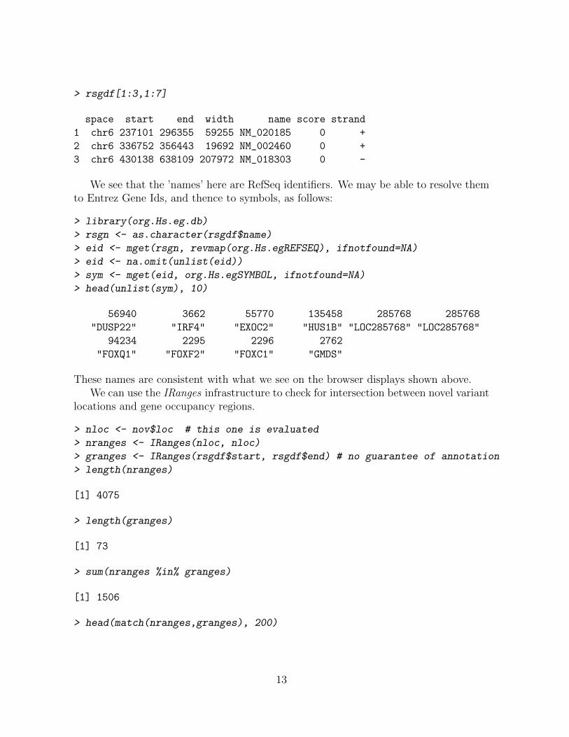
> rsgdf[1:3,1:7]

space start end width name score strand

1 chr6 237101 296355 59255 NM_020185 0 +

2 chr6 336752 356443 19692 NM_002460 0 +

3 chr6 430138 638109 207972 NM_018303 0 -

We see that the ’names’ here are RefSeq identifiers. We may be able to resolve themto Entrez Gene Ids, and thence to symbols, as follows:

> library(org.Hs.eg.db)

> rsgn <- as.character(rsgdf$name)

> eid <- mget(rsgn, revmap(org.Hs.egREFSEQ), ifnotfound=NA)

> eid <- na.omit(unlist(eid))

> sym <- mget(eid, org.Hs.egSYMBOL, ifnotfound=NA)

> head(unlist(sym), 10)

56940 3662 55770 135458 285768 285768

"DUSP22" "IRF4" "EXOC2" "HUS1B" "LOC285768" "LOC285768"

94234 2295 2296 2762

"FOXQ1" "FOXF2" "FOXC1" "GMDS"

These names are consistent with what we see on the browser displays shown above.We can use the IRanges infrastructure to check for intersection between novel variant

locations and gene occupancy regions.

> nloc <- nov$loc # this one is evaluated

> nranges <- IRanges(nloc, nloc)

> granges <- IRanges(rsgdf$start, rsgdf$end) # no guarantee of annotation

> length(nranges)

[1] 4075

> length(granges)

[1] 73

> sum(nranges %in% granges)

[1] 1506

> head(match(nranges,granges), 200)

13

[1] NA NA NA NA NA NA NA NA NA NA NA NA NA NA NA NA NA NA NA NA NA NA NA NA NA




[101] NA NA NA NA NA NA NA NA 1 1 1 1 1 1 1 1 1 1 1 1 1 1 1 1 1

[126] 1 1 1 1 1 NA NA NA NA NA NA NA NA 2 2 NA NA NA NA NA NA NA NA NA NA



We can see that there is a batch of variants present in the first gene, and this is confirmed

14

by checking the 1KG browser.

Looking in more detail, we have

15

and this can be exploded into the Ensembl variant browser view

with textual metadata view

16

So it seems DUSP22 resides over plenty of known SNP; our computations are sup-posed to reveal hitherto unknown variants in this region for this individual.

5.3 Exercises

1. The oregdf data.frame is supplied in ind1KG , containing information on regula-tory elements annotated in oreganno. How many novel variants for NA19240 liein oreganno regulatory regions? What types of regions are occupied?

2. Derive a data.frame for regions of nucleosome occupancy in our 10 Mb segmentand check how many of the novel variants lie in such regions.

17

exploring data from the 1000 genomes project in ... · exploring data from the 1000 genomes project...

Documents