Paper SD12

Page 1 of 19

Exploring Cellular Automata

Daniel Olguin, First Coast Service Options, Jacksonville, FL

ABSTRACT

In 1970 Martin Gardner brought cellular automata to the attention of the general public with a Scientific American article on a ‘game’ created by mathematician John Conway called the ‘Game of Life’. In 2004, Stephen Wolfram declared cellular automata to be the basis of ‘A New Kind of Science’. This paper will explore those cellular automata and various techniques for presenting them using SAS Graphics capabilities.

INTRODUCTION

I like to read, and being a programmer by trade, when I come across something interesting, I like to see, if and how, I can produce it in whatever programming language/environment I'm working with at the moment. Being new to SAS Graphics capabilities, I wanted to see if I could reproduce various diagrams on 1 dimensional Cellular Automata as presented in 'A New Kind of Science' by Stephen Wolfram. This paper will start by covering what I learned about SAS Graphics while trying to achieve that goal. I'll follow that up by going over SAS Graphics techniques for animation using 'The Game of Life' (a 2D Cellular Automata) to provide the fun.

CELLULAR AUTOMATA

Cellular Automata (CA) are a type of simulation. They are generally represented by a grid of cells/squares in one or two dimensions (1D/2D); for 2D, think graph-paper or checkerboard. Each cell/square has neighbors. What constitutes a neighbor can vary between automatons but applies equally to every cell in an automaton. The neighbors are important because the relationship between a cell and its neighbors determines the various changes in state of a cell (much like the absence of close neighbors among the early settlers or the over-crowding of a modern city like New York). Each change of state is dictated by a set of rules for the automaton. All of the rules are applied simultaneously in discrete time steps or ticks. The universal state of an automaton after a tick is a generation.

In summary a CA can be thought of as:

1) A grid (1D/2D)

2) Of cells/squares

3) Each cell having neighbors

4) Which determine the state of the cell

5) Through the application of rules

6) Applied at discrete time intervals

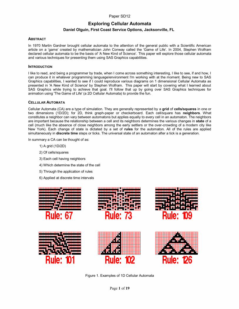
Figure 1. Examples of 1D Cellular Automata

Paper SD12

Page 2 of 19

1D CAs

Below is an example of a 1D CA of the type studied by Stephen Wolfram. It's one-dimensional (1D) with each row representing a generation. The rows can be thought of as infinite both to the left and the right. Each successive row is a new generation determined by applying the rule (in this case, Rule 126) to the cells in the immediately preceding row/generation. What's striking about this automaton is the obvious structural complexity generated by a simple initial state (a single occupied cell) acted upon by simple rules.

Note: For those familiar with fractals note the remarkable similarity to a Sierpinski triangle!???

Figure 2. A 1D CA Rule 126

This cellular automaton can be described by its rule, 126. In base 2 that's 01111110. Each bit having a value 1 indicates where a cell will become or remain occupied. Each bit having a value of 0 indicates where a cell will become or remain unoccupied. Each bit position applies to a different arrangement of neighboring cells in the current generation.

Using the above figure as an example and starting at the first row/generation, each cell (excluding the 3 cells in the center) have a neighborhood which is (empty,empty,empty) or (000). That neighborhood maps to the first bit on the right of Rule 126 which is bit 0 (01111110). Since the value of the rule at bit 0 is '0' the succeeding generation is empty. Which is why most of generation 1 (i.e. the second row from the top) is empty.

The 3 cells in the middle (because of their differing neighborhoods) are handled by different parts of the rule. The neighborhoods are always the cell being examined (current) and it's 2 neighbors, left and right ; given as (L,C,R).

The left most of the 3 cells in the middle of generation 0 has the neighborhood (empty, empty, occupied) or (001) which maps to bit 1 (01111110) of the rule. Since bit 1 of the rule has a value of 1 the succeeding generation is occupied.

The middle cell of generation 0 is the only occupied cell. It's neighborhood is (empty, occupied, empty) or (010) which maps to bit 2 (01111110) in the rule. Since bit 2 of the rule has a value of 1 the succeeding generation is occupied.

Finally, the right most of the middle 3 cells has a neighborhood of (occupied, empty, empty) or (100) which maps to bit 4 (01111110) of the rule. Since bit 4 of the rule has a value of 1 the succeeding row is occupied. That gives us generation 1 (second row from the top) with 3 occupied cells in the center.

The process is repeated to determine any number of succeeding generations.

Paper SD12

Page 3 of 19

We'll see how to use DSGI to generate graphics like Figure 2 with a little help from Proc GANNO to produce the rules.

DATA Step Graphics Interface (DSGI)

DSGI as its name implies allows you to create graphics from within a Data Step. DSGI output is stored in a catalog which is work.gseg by default. Data Steps using DSGI must follow a specific structure:

1)rc = ginit(); * Initializes DSGI;

2)rc = graph('clear', graphName); * Opens a Graphics Segment;

3)/* Your graphics code here */

4)rc = graph('update'); * Update the catalog ;

5)rc = gterm(); * End the DSGI session;

Warning! A graphName must be 8 or less characters.

1DCA.sas (partial listing)

goptions reset=all colors=(red green blue black white) device=gif ;

data _null_;

retain RED 1 GREEN 2 BLUE 3 BLACK 4 WHITE 5;

* Initializes DSGI;

rc = ginit();

graphName = '_1DCA';

* Opens a Graphics Segment;

rc = graph('clear', graphName);

* Generation 0;

if _n_ = 1 then link Setup;

do t = 1 to &generations;

link ApplyRules;

cur_gen = nxt_gen;

end;

* Update the catalog with this segment;

rc = graph('update');

* End the DSGI session;

rc = gterm();

stop;

/* Linked subroutines follow */

In the code for 1DCA.sas above, the core of the application code is the link to Setup, for Generation 0 (zero), and the do loop for generations. All Cellular Automata have an analogous structure at the highest level of abstraction. The surrounding statements are the obligatory DSGI scaffolding.

Paper SD12

Page 4 of 19

Besides the DSGI functions ginit, graph, and gterm, there are functions to set attributes (GSET) and functions to draw (GDRAW). There are also DSGI routines (GASK) to query the various attributes of the graphics environment.

Within Setup (a subroutine in our program 1DCA.sas), we

1) Use the GASK function to ask about the current Window attributes in order to calculate the cellHeight and cellWidth.

2) Initialize our data structures cur_gen and next_gen as simple strings to hold the current and next generations

3) Finally we display Generation 0

Setup:

row = 1;

call gask('WINDOW', 0, llx, lly, urx, ury, rc);

* UpperRightY (ury) / desired #of rows;

cellHeight = int((ury / &rows));

* UpperRightX (urx) / desired #of cols;

cellWidth = int((urx / &cols));

half = int(&cols / 2);

cur_gen = repeat('0',half) || '1' || repeat('0',half);

nxt_gen = strip(cur_gen);

link DefaultFill;

do;

y = int(ury)- cellHeight;

link DisplayGeneration;

row = row + 1;

end;

return;

DSGI offers a number of graphics (GDRAW) primitives, 3 of which we'll need; line, bar, and text. Prior to using DSGI drawing functions to generate our graphics, we'll set the fill color and fill type attributes using GSET functions. Since the cells of the automata start out empty, the default filtype we'll use is 'HOLLOW'. An unoccupied cell will be empty ('HOLLOW') with a RED border. An occupied cell will be ‘SOLID' BLACK with a RED border.

DefaultFill:

rc=gset('filtype', 'HOLLOW');

rc=gset('filcolor', RED);

return;

Paper SD12

Page 5 of 19

To display a Generation we simply iterate through the nxt_gen data structure drawing each cell as appropriate.

DisplayGeneration:

x = 0;

do col = 1 to &cols;

if substr(nxt_gen,col,1) = '1' then link SolidFill;

else link DefaultFill;

link DrawCell;

x = x + cellWidth;

end;

The output from 1DCA.sas for Generation 0 should look something like:

Figure 3. 1DCA.sas output for Generation 0

The do loop for t (i.e. time or tick) simply applies the Rules to produce the next generation.

ApplyRules:

do;

y = y - cellHeight;

do col = 1 to &cols;

link GetNeighborhood;

if band(rule,2**neighborhood) then substr(nxt_gen,col,1) = 1;

else substr(nxt_gen,col,1) = 0;

end;

link DisplayGeneration;

row = row + 1;

end;

return;

The key to ApplyRules is in 2 parts; the neighborhood and the application of the rule using band. The neighborhood is 3 bits representing the left neighbor, current cell, and right neighbor, with bit value '1' meaning occupied, and bit value '0' unoccupied. The band function compares the parameters bit by bit returning a 1 in that bit position if both parameters have a 1 else returning a zero. The reason for raising 2 to the power of neighborhood (

2**neighborhood) is that the resulting number has exactly 1 bit with a value of '1' which corresponds to the bit

position of the rule for which the neighborhood applies!

Paper SD12

Page 6 of 19

A few small modifications to the original code gives us the ability to generate all 256 automatons.

1DCA.sas (partial with modifications)

.

.

.

rc = ginit();

do rule = 0 to 255; * NEW ;

graphName = '_1DCA' || strip(put(rule,3.)); * Modified;

rc = graph('clear', graphName);

link ShowRule;

if _n_ = 1 then link Setup;

do t = 1 to &generations;

link ApplyRules;

cur_gen = nxt_gen;

end;

rc = graph('update');

end; * End do rule; * NEW;

rc = gterm();

Each of the graphics is named '_1DCArule' where rule is a number 0 through 255. By default they have been placed in catalog, work.gseg. They can be listed with the following code (taken from a SAS sample):

%macro listcat(catname);

%if %sysfunc(cexist(&catname)) %then %do;

proc greplay nofs igout=&catname;

list igout;

run;

%end;

quit;

%mend ;

%listcat(work.gseg);

Paper SD12

Page 7 of 19

Or deleted from the catalog with this code (again taken from a SAS sample):

%macro delcat(catname);

%if %sysfunc(cexist(&catname)) %then %do;

proc greplay nofs igout=&catname;

delete _all_;

run;

%end;

quit;

%mend ;

%delcat(work.gseg);

So far we can generate all 256 of the automatons similar to Figure 2 but we're still missing the display of the Rules. For that we'll switch our attention to Proc GANNO.

Proc GANNO

The GANNO procedure displays graphs by reading Annotate datasets having a specific format in terms of the names and types of columns in the dataset(s). Each row in the dataset represents a command or action. Our graphics requirements remain the same as when we were using DSGI; i.e. we need to be able to draw rectangles, lines, and text.

As an example of what we'll try to draw, look at Figure 4.

Figure 4. Rule 1

We have a bottom row of text (Rule: 1 = 00000001) and above it a collection of rectangles, both filled and unfilled, relating the neighborhoods to the rule bit.

The complete code for 1DCARules.sas is located at the bottom of the paper. Most of the code is simply related to positioning the various elements of the graphic and not particularly interesting. So we'll focus on the few elements related to GANNO and Annotate datasets.

A commonly repeated pattern in generating data for an Annotate dataset is a function assignment followed by a series of assignments regarding attributes of the function and terminated by an output statement.

The example below has a function move with calculated lower left x/y coordinates which is outputted. The next line is for the function 'bar' which will draw a rectangle in black from the lower left of the 'move' to the new x/y.

function='move'; x=(c-1)*width+1; y=(r-1)*height; output;

function='bar'; x=x+width-.5; y=y+height-1; color='black'; output;

Paper SD12

Page 8 of 19

So, whereas DSGI generates the graphic directly in the data step, here we build an intermediate dataset of commands which we'll pass to Proc GANNO.

A few lines of Proc Ganno code take our Annotate dataset and creates the graphic and stores it in the work.gseg catalog (thanks to the gout= argument). Note that we also supplied a name= argument to control the naming of each graph, as we'll need to reference them shortly.

proc ganno anno=_1DCARule&rule gout=work.gseg name="car&rule" datasys;

run;

quit;

We now have a complete set of Rules Graphics thanks to 1DCARule.sas.

We return to 1DCA.sas to complete our 1DCA related example.

To add the rules generated by 1DCARules.sas to our graphic generated by DSGI, we add the following:

1DCA.sas (new addition)

ShowRule:

rc=gset('viewport', 1, .3, 0, 1,.2);

rc=gset('transno',1);

r = 'car' || strip(put(rule,3.)); put r=;

rc=graph('insert',r);

put rc=;

rc=gset('viewport', 2, 0,0,1,1);

rc=gset('transno',2);

return;

The gset('viewport' sets part of the graphic area starting at the lower left at (.3,0) to (1,.2); which is to say a rectangular area whose lower left is at 30% along the X axis and 0% on the Y axis to the upper right being 100% of the X axis and 20% of the Y axis.

The gset('transno' says that subsequent graph commands will apply to the viewport numbered 1.

The rule name, r, is derived and used in the graph('insert' command. Notice that the name begins 'car' followed by the rule number. That's the naming convention we used in generating the graphic with Proc GANNO (see Proc GANNO code above on this page).

The gset('viewport',2 designates 100% of the drawing area and the gset('transno makes it available for the next series of graphics commands.

We can now produce 1DCAs at will with their associated rules.

But wait there's more!

On page 55 of his book 'A New Kind of Science', Stephen Wolfram displays a full page of automata as thumbnails much like what you see on the next page.

Paper SD12

Page 9 of 19

Can we do this in SAS?

Figure 5. A page of 1DCAs

Paper SD12

Page 10 of 19

The answer (as if there was any doubt) is yes!

We first make a small change to 1DCA.sas to construct a purely text rule, as at thumbnail size, the graphic rule is not legible (and Wolfram makes the same change).

ShowRule:

if "&thumbnails" = "Y" then

do;

r = 'Rule: ' || strip(put(rule,3.));

rc=gset('texfont','swissb');

rc=gset('texheight',15);

rc=gdraw('text', 15,60, r);

end;

else

do;

rc=gset('viewport', 1, .3, .5, 1,.7);

rc=gset('transno',1);

r = 'car' || strip(put(rule,3.));

rc=graph('insert',r);

put rc=;

rc=gset('viewport', 2, 0,0,1,1);

rc=gset('transno',2);

end;

return;

Paper SD12

Page 11 of 19

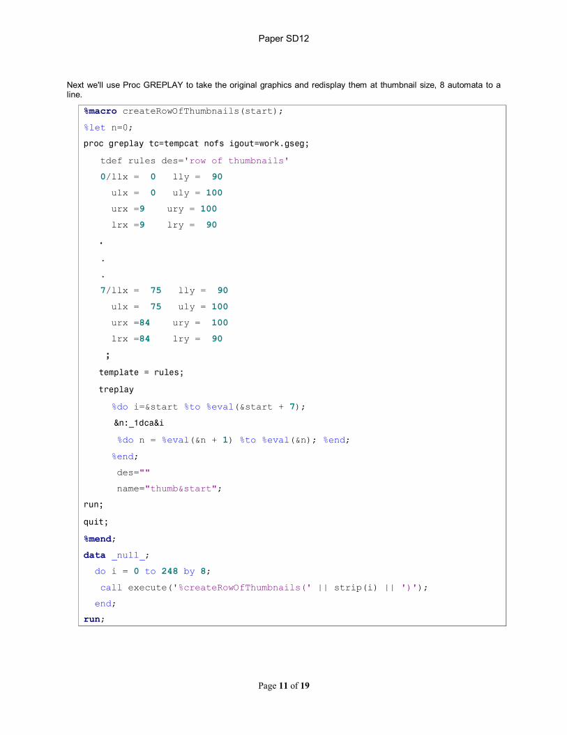
Next we'll use Proc GREPLAY to take the original graphics and redisplay them at thumbnail size, 8 automata to a line.

%macro createRowOfThumbnails(start);

%let n=0;

proc greplay tc=tempcat nofs igout=work.gseg;

tdef rules des='row of thumbnails'

0/llx = 0 lly = 90

ulx = 0 uly = 100

urx =9 ury = 100

lrx =9 lry = 90

.

.

.

7/llx = 75 lly = 90

ulx = 75 uly = 100

urx =84 ury = 100

lrx =84 lry = 90

;

template = rules;

treplay

%do i=&start %to %eval(&start + 7);

&n:_1dca&i

%do n = %eval(&n + 1) %to %eval(&n); %end;

%end;

des=""

name="thumb&start";

run;

quit;

%mend;

data _null_;

do i = 0 to 248 by 8;

call execute('%createRowOfThumbnails(' || strip(i) || ')');

end;

run;

Paper SD12

Page 12 of 19

We use Proc GREPLAY a second time to take each row of thumbnails and redisplay them 16 rows to a page.

%macro createPage(start);

%let n=0;

proc greplay tc=tempcat nofs igout=work.gseg;

tdef rules des='a page of thumbnails'

0/llx = 0 lly = 0

ulx = 0 uly = 100

urx =100 ury = 100

lrx =100 lry = 0

1/llx = 0 lly = 0

... same as 0/ ...

lrx =100 lry = 0

xlatey=-5

2/llx = 0 lly = 0

... same as 0/ ...

lrx =100 lry = 0

xlatey=-10

.

.

.

16/llx = 0 lly = 0

... same as 0/ ...

lrx =100 lry = 0

xlatey=-80 ;

template = rules;

treplay

%do i=&start %to %eval(&start + 120) %by 8;

&n:thumb&i

%do n = %eval(&n + 1) %to %eval(&n); %end;

%end;

name="test";

run;

quit;

%mend;

%createPage(0);

Which produces the full page of 1DCAs in Figure 5 on page 9.

Paper SD12

Page 13 of 19

Recap

1) We've used DSGI to generate one dimensional cellular automata.

2) We then used Proc GANNO to generate a graphic version of the automata rules

3) We modified our original program to include the rule graphic

4) We finished off by using Proc GREPLAY to create a page full of automata as thumbnails

We're now going to leave behind 1DCAs and move into 2 dimensions. We'll also be moving from static displays to animation.

In Two Dimensions

Cellular Automata are not limited to 1 dimension. In fact the history of cellular automata theory began in the 1950s under John von Neumann when he sought to determine if machines could self-replicate. Von Neumann's, 'uniform cellular space', can be visualized as an infinite grid. Each cell in the grid can be occupied or empty. The cells change state as a result of simple transition rules based on the state of neighboring cells. Von Neumann achieved his existence proof with an automaton of cells with 29 states, four neighbors and a configuration of 200,000 cells.

The Game of Life

In 1970, Martin Gardner published an article in Scientific American describing the research of, John Conway, a mathematician at the University of Cambridge which has become what is probably the most famous of cellular automata, 'The Game of Life'.

Conway was looking for cellular automata that were both interesting and unpredictable. He had 3 constraints designed to produce those goals:

1) That there would be no simple proof that an initial pattern would grow without limit.

2) That there should be some initial patterns that appeared to grow without limit.

3) That there should exist simple initial patterns that grow and change for a time but that eventually die out or end in oscillations.

Conway tried many variations finally settling on 3 simple genetic laws

1) The occupant of a cell survived if it had 2 or 3 neighbors

2) The occupant of a cell died if it had 1 or fewer neighbors or 4 or more neighbors

3) Lastly, an empty cell had a birth if it had exactly 3 occupied neighboring cells

All the laws are applied simultaneously at each 'tick' (time event). Each tick represents the start of a new generation, the result of the rules being applied to the prior generation.

Paper SD12

Page 14 of 19

The core of the program GOL.sas, is as follows:

GOL.sas (partial listing)

if _n_ = 1 then link Setup;

do t = 1 to &generations;

link Survival; * Determine the survivors. Rule 1;

* And Deaths. Rule 2;

link Birth; * Determine the births. Rule 3;

link Death; * Eliminate the dead.;

link SaveGen; * Save the generation.;

end;

Note the similarity to the core of 1DCA.sas. There is a Setup subroutine to initialize generation 0. We use hashes for data structures rather than strings as in the 1D version.

Setup: (partial listing)

do;

link CurrentAttributes; * For graphics;

/* gol (Game of Life) hash will keep track of the living */

length living 3. d 3.;

declare hash gol();

declare hiter iter('gol');

gol.definekey('r', 'c'); * r=row,c=col of grid;

gol.definedata('r', 'c', 'living');

gol.definedone();

call missing(living);

do until(eof);

set work.&input end=eof; * A generation 0;

living = 1;

link Initialize;

end;

/* Save the Initial Generation - Gen0 */

t=0;

link SaveGen;

...

return;

Paper SD12

Page 15 of 19

Survivors and deaths are calculated by iterating over the current living and applying Rules 1 and 2.

Survival:

/* Occupied with 2 or 3 neighbors Survives else Dies */

rc = iter.first();

do while (rc = 0);

link Neighbors; * Returns the number of neighbors (n);

if n = 2 or n = 3 then ; * Survivor; else Mark the death.

else rc = gol.replace(key: r, key: c, data: r, data: c, data: 0);

rc = iter.next();

end;

return;

Births are determined by iterating over both the Survivors and those marked for death. Note that, parents, was cacluated when the subroutine, Neighbors, was executed in calculating the survivors.

Birth:

/* An empty cell with 3 parents (i.e. 3 occupied neighboring cells) */

rc = biter.first();

do while (rc = 0);

if parents = 3 then

do; * This is a birth!;

rc = gol.add(key: row, key: col, data: row, data: col, data: 1);

end;

pr=row; /* Prior row */

pc=col; /* Prior col */

rc = biter.next();

rc = births.remove(Key: pr, Key: pc);

end;

return;

Paper SD12

Page 16 of 19

Another advantage of using a hash to hold the generation is that it provides an easy mechanism for saving the data to a dataset for future processing.

SaveGen:

genDSName = 'work.gen' || strip(t);

rc = gol.output(dataset: genDSName);

if rc = 0 then output;

return;

I use a simple routine for the creation of the initial generation. Asterisks represent an occupied cell; spaces (or any other character), unoccupied. The data step assigns row (r) and column (c) positions to each occupied cell and discards the rest. The following example loads all the possible 3 cell creatures (rotations are not material).

data work.triplets;

infile datalines truncover;

drop row;

input row $char100.;

r = _n_;

do c = 1 to 100;

if substr(row, c, 1) = '*' then output;

end;

datalines;

* * * ** ***

* * * * *

* *

;

run;

We're now in a position to produce any number of generations given a generation 0. All well and good, but not very exciting nor informative. To really appreciate the 'Game of Life', one has to see it in action. To do so we need to choose a presentation mechanism. We used DSGI for the 1DCA demo so this time we'll turn to Proc GANNO and javameta.

Paper SD12

Page 17 of 19

We'll need a 2 dimensional grid. Since we're going to use Proc GANNO to generate the graphic, we'll need a data step program to create the Annotate dataset containing instructions to draw a grid of cells. We've already seen how that can be done by using do loops to generate a series of 'move' and 'draw' commands.

GenerateGrid.sas (excerpt)

...

do r = 0 to &cells;

function='move'; x=0; y=(r*step); output;

function='draw'; x=&max; color='black'; output;

end;

...

We now have our generations created by GOL.sas and our grid created by GenerateGrid.sas. We merge the two with a macro %DisplayGen, which produces another Annotate dataset which is the input for Proc GANNO.

%macro DisplayGen(genDS);

...

data gol;

set work.grid (in=a) &genDS (in=b) end=eof;

...

run;

...

proc ganno anno=work.gol datasys;

run;

quit;

%mend;

The driver which calls the DisplayGen macro, sets the environment to produce javameta output.

DisplayGenDriver.sas (partial listing)

ods _ALL_ close;

ods listing; *allows metacodes to be written to _webout;

goptions reset=all device=javameta ;

/* When goptions device=javameta, the output of the procedure

* goes to webout

*/

Filename _webout “&webout”;

…

Paper SD12

Page 18 of 19

Now all you need is to create a html page that will use the SAS Metaview Applet to display the metacodes.

GOL.html (complete listing)

<!DOCTYPE HTML PUBLIC "-//W3C//DTD HTML 4.0 Transitional//EN">

<html>

<head><title>Game of Life</title></head>

<body>

<applet archive="file:///C:\Program Files\SAS\SAS Learning Edition

4.1\common\applets\metafile.zip"

code="MetaViewApplet.class"

width="800" height="550" align="TOP">

<param name="BackgroundColor" value="0x000000">

<param name="ZoomControlEnabled" value="true">

<param name="SlideShowControlEnabled" value="true">

<param name="Metacodes" value="http://NET20/BI/r_pentomino.txt">

<param name="MetacodesLabel" value="1993">

Sorry, your browser does not support the applet tag

</applet>

</body>

</html>

The points of interest are:

1)The archive= argument. Points to the metafile.zip which is a SAS supplied component. (Location is specific to your environment!)

2)The code= argument. Identifies the applet to use. (Don't change this argument.)

3)The <param> ZoomControlEnabled and SlideShowControlEnabled. Used respectively to zoom in and out and to control the animation.

4)The <param> Metacodes, which points to the location of the file you created; i.e. File _webout from DisplayGenDriver.sas. (Specific to your environment!)

You can now spend countless hours viewing the life forms of your creation! Have fun!

CONCLUSION

We've taken a look at one and two dimensional cellular automata. Along the way we've explored (but briefly) various SAS tools for generating graphics outside of the standard business graphics like line, bar, and pie charts. We've seen how DSGI can be used in the data step to directly generate graphics as well as include graphics generated elsewhere. We've also constructed graphics by generating Annotate datasets which we fed to Proc GANNO. We've used Proc GREPLAY to reposition and resize groups of graphics to produce elaborate page displays. Finally, we've used javameta and the Metaview applet to produce controllable animations.

Paper SD12

Page 19 of 19

REFERENCES

SAS/Graph 9.1 References Vol 1-3

see also the titles in the Recommended Readings list

RECOMMENDED READING

A New Kind of Science, Stephen Wolfram, Wolfram Media, Inc. 2002

Wheels, Life And Other Mathematical Amusements, Martin Gardner, W.H. Freeman and Company, 1983

The Recursive Universe, William Poundstone, Contemporary Books Inc., 1985

CONTACT INFORMATION

Your comments and questions are valued and encouraged. Contact the author at:

Daniel Olguin 2408 Spring Vale RD Jacksonville, FL 32246 E-mail: olguind@bellsouth.net

SAS and all other SAS Institute Inc. product or service names are registered trademarks or trademarks of SAS Institute Inc. in the USA and other countries. ® indicates USA registration.

Other brand and product names are trademarks of their respective companies.

Complete Program Listings may be downloaded from http://olguind.clearwire.net/downloads