explorign computer vision in deep learning: object detection and … · 2019-04-24 · specifically...
TRANSCRIPT

1
Paper SAS3317-2019
Exploring Computer Vision in Deep Learning: Object Detection and
Semantic Segmentation Xindian Long, Maggie Du, and Xiangqian Hu, SAS Institute Inc., Cary, NC
ABSTRACT
This paper describes the new object detection and semantic segmentation features in SAS
Deep Learning, which are targeted to solve a wider variety of problems that are related to
computer vision. The paper focuses on algorithms that are supported on SAS® Viya®,
specifically Faster R-CNN and YOLO (you only look once) for object detection, and U-Net for
semantic segmentation. This paper shows how to use the functionality of the Deep
Learning action set in SAS® Visual Data Mining and Machine Learning in addition to DLPy,
an open-source, high-level Python package for deep learning. The paper demonstrates
applications of object detection and semantic segmentation on different scenarios, and it
shows how to prepare data, build networks, select parameters, load or train the weights,
and display results. Future development and potential applications in different areas are
discussed.
INTRODUCTION
Computer vision is about understanding the visual world around us through digital images
and videos. In applications such as self-driving cars, production line automation, face
recognition, and medical image processing, computer software analyzes the image content
and accomplishes one or several of the following basic tasks: image classification, keypoints
detection, object detection, segmentation, and so on. Briefly, image classification represents
the task of given an image, discovering the main content in the image. Object detection
locates the positions and categories of objects in a given image. Semantic segmentation
classifies the pixel-level category assignments, while instance segmentation, assigns
different labels for pixels belong to different instances of the same object type.
Traditionally, computer vision tasks are accomplished by manually designed features,
including Gabor filter, Gaussian filter, Scale Invariant Feature Transform (SIFT) filter, and so
on. Recently, Deep Learning (that is, deep neural networks) has been proven to boost the
field tremendously. Not only can computers complete the above tasks much faster, more
accurately, but also with little human crafted features since these features are learned
automatically using the input data.
SAS Viya® supports computer vision through SAS Deep Learning with features including
image classification, keypoints detection, object detection, and semantic segmentation. For
all these features, two interfaces are available:
• CAS (Cloud Analytic Services) actions: These give users more granular control over
the various options.
• DLPy (https://github.com/sassoftware/python-dlpy): It has a Keras-type Python interface with a
higher abstraction.
From this paper, you will learn how to use the features of object detection and semantic
segmentation by working through some real-world examples. The object detection examples
use different CAS actions through our CAS action set python programming interface, while
the semantic segmentation is illustrated through DLPy.
OBJECT DETECTION

2
Object detection analyzes complex images that contain a mixed multitude of objects, at
different distances and locations, amidst varying, often visually noisy backgrounds. Objects
can appear anywhere within the visual frame, be near or far, and can overlap with each
other. Object detection locates and classifies unknown objects, as well as determining their
boundaries as shown in Figure 1.
Figure 1. The Concept of Object Detection
Object detection is a challenging and one of the most fundamental tasks in computer vision.
Lately CNN (Convolutional Neural Networks) based deep learning algorithms like YOLO [1]
(You only look once), SSD [2] (Singleshot multibox detector), R-CNN [3] (Region proposal
networks), Faster R-CNN [3], RetinaNet [4], and so on, have been implemented to address
this problem and have been very successful.
Object detection algorithms can be categorized as below:
1. The first algorithm category is to do region proposal first. This means regions highly
likely to contain an object are selected either with traditional computer vision techniques
(like selective search), or by using a deep learning based region proposal network
(RPN). Once you have gathered the small set of candidate windows, you can formulate a
set number of regression models and classification models to solve the object detection
problem. This category includes algorithms like Faster R-CNN, R-FCN [5], and FPN-FRCN
[6]. Algorithms in this category are usually called two-stage methods. They are
generally more accurate, but slower than the single-stage method introduced below.
2. The second algorithm category only looks for objects at fixed locations with fixed sizes.
These locations and sizes are strategically selected so that most scenarios are covered.
These algorithms typically separate the original images into fixed size grid regions. For
each region, these algorithms try to predict a fixed number of objects of certain, pre-
determined shapes and sizes. Algorithms belonging to this category are called single-
stage methods. Examples of such methods include YOLO, SSD, and RetinaNet.
Algorithms in this category usually run faster but are less accurate. This type of
algorithm is often used for applications requiring real-time detection.
SAS deep learning supports two representative algorithms, Faster R-CNN and YOLO, which
belong to the two above algorithm categories respectively.
YOLO

3
YOLO (You Only Look Once) is the representative algorithm in single-stage object detection
method. The steps it follows to detect objects are represented in Figure 2 and in the list
below:
Figure 2 Steps illustrating the YOLO Algorithm
1. Separate the original image into grids of equal size.
2. For each grid, predict a preset number of bounding boxes with predefined shapes
centered around the grid center. Each prediction is associate with a class probability and
an object confidence (whether it contains an object, or it is just the background).
3. Finally, select those bounding boxes associated with high object confidence and class
probability. The object category is the object class with the highest class probability.
The preset number of bounding boxes with pre-defined shapes are called anchor boxes.
They are obtained from the data by the K-means algorithm. The anchor box captures prior
knowledge about object size and shape in the data set. Different anchors are designed to
detect objects with different sizes and shapes.
For example, in Figure 3, there are three anchors at one location. The red anchor box turns
out to detect the person in the middle. In other words, the algorithm detects the object with
the approximate size of this anchor box. The final prediction is usually different from the
anchor location or size itself; an optimized offset obtained from the feature map of the
image is added to the anchor location or size.
Figure 3 Anchor Boxes

4
FASTER R-CNN
Faster R-CNN is a two-stage object detection algorithm. Figure 4 illustrates the two stages
in Faster R-CNN. Although “faster” is included in the algorithm name, that does not mean
that it is faster than the one-stage method. The name is a historical artifact – it simply
indicates that it is faster than it is previous versions, the original R-CNN [7] algorithm, and
the Fast R-CNN [8], by sharing the computation of feature extraction for each region of
interest (RoI), and by introducing the deep learning-based region proposal network (RPN).
After using many CNN layers to extract feature maps, the region proposal network (RPN)
generates many windows that are highly likely to contain an object. The algorithm then
retrieves the feature maps inside each window, resizes (or polls) them into fixed sizes (RoI
pooling), and predicts the class probability and a more accurate bounding box for the
object.
One question to consider is how the RPN generates these windows. Like YOLO, RPN also
uses anchor boxes. Unlike YOLO, the anchor boxes are not generated from data but instead
are of fixed sizes and shapes selected strategically to cover main object shapes and sizes.
The anchor boxes can also cover the image more densely. Note that instead of performing a
classification on many object categories, the RPN only does a binary classification on
whether the window contains an object or not.
Figure 4 Stages in the Faster R-CNN Object Detection Algorithm
Picture from the Original Faster R-CNN Paper [3]
BUILD DEEP LEARNING MODELS
Building and using any deep learning model involves four steps illustrated in Table 1. In the
following sections, you can see how these steps are completed using SAS deep learning
toolkit.

5
1. Preparing and Loading the Data
2. Building the model architecture, namely, the model DAG (Directed Acyclic Graph)
consisting of many layers.
3. Loading or Training the weights
4. Inference and Visualization
Table 1 Steps in Building and Using a Deep Learning Model
DATA EXPLORATION AND PREPARATION
An essential part of any data science project is to explore the data, complete any pre-
processing if needed, and prepare it for training or inferences. CAS provides toolsets to help
you through the process.
Images and Labels
The images and label data need to be organized into a CAS table before training or scoring.
Each image can contain more than one labeled object. Each label should contain the object
category and the object bounding box.
In this paper, we assume images and associated labels are already joined and put in a CAS
table. In the table there is a column for the image, and there are many columns for
bounding box and category labels. Figure 5 shows some records for the table trainset.
Figure 5 The Joined Table Containing Images and Labels
Data Format
In Figure 5, you can see that for record 598, there are two labeled objects, as shown in the
_nObjects_ column; the first object category, and bounding box location is stored in
columns _Object0_, _Object0_x, _Object0_y, _Object0_width,
_Object0_height. The values in location columns in the table are smaller than 1,
because they are in YOLO format, which are normalized according to the input image size.
YOLO is the recommended format since it is easier to do data augmentation with it.
Visualize the Images and Labels
To check if your label is correct visually, you can use the extractDetectedObjects action
to extract the object location/category and generate images with the bounding boxes, class
names, and score values (when the table is the output of the dlscore action), annotated on
the image.

6
s.image.extractdetectedobjects
(casout={'name':'trainSetAnnoted','replace':True},
coordType=’Yolo’, maxobjects=30, table=s.CASTable(‘trainSet’))
Figure 6 shows the annotated images generated.
Figure 6 Images and Annotations: The Bounding Boxes and Categories
BUILDING THE MODEL ARCHITECTURE
The Backbone Network
Both YOLO and Faster R-CNN Object Detection model need a backbone network to extract
features from the images. The backbone network typically is a well-known network used for
image classification, for example, ResNet, VGG16, Darknet, and so on. The backbone
network usually consists of the data layer, many convolutional layers, batch normalization
and pooling layers.
Table 2 shows how you connect to a CAS server, load the action sets needed, create a CNN
model with name TinyYOLO and add layers to build the backbone network for the model.
Only the first few layers and the last layer for the backbone network is shown for simplicity.
import swat # The python interface to SAS Cloud Analytic Services (CAS).
s = CAS('cas04.unx.sas.com', 29990) # connect to the CAS server
s.loadactionset('image') # load the image action set
s.loadactionset('deepLearn') # load the deep learning action set
s.buildModel(model=dict(name=‘TinyYOLO’,replace= True),type=CNN')
s.addLayer(model=modelName, name='data',
layer=dict(type='input', nChannels=3,width=imgWidth,
height = imgHeight, scale = 1.0/255))
s.addLayer(model=modelName, name='conv1',
layer=dict(type='convolution', nFilters=16, width=3, height=3,
stride=1, includeBias=False, std=1e-1, act='identity'),
srcLayers = ['data'])
s.addLayer(model=modelName, name='bn1',
layer=dict(type='batchnorm', act='leaky'),
srcLayers = ['conv1'])
s.addLayer(model=modelName, name='pool1',

7
layer=dict(type='pooling',width=2, height=2,stride=2, pool='max'),
srcLayers = ['bn1']
……
s.addLayer(model=modelName, name='conv9',
layer=dict(type='convolution', nFilters=125,
width=1, height=1, # filter width and height
stride=1, includeBias=False, std=1e-1, act='identity'),
srcLayers = ['bn8'])
Table 2 Code Snippet to Build the Backbone Network for YOLO Object Detection Model
The YOLO Detection Layer
Table 3 shows how to add the YOLO detection layer following the last layer of the backbone
network, and some typical parameters used. In the last convolutional layer conv9, the
width and height of the output feature map should both equal to gridNumber (13), and the
depth (nFilters) should be equal to:
predictionsPerGrid * (classNumber + coordNumber + 1),
in which gridNumber, predictionsPerGrid, classNumber are parameters in the detection
layer, and coordNumber is equal to 4, which is the number of values needed to represent a
rectangle bounding box. Anchors are given directly here, which is pre-calculated using K-
means algorithm. DLPy provides a function helping you to calculate proper anchors from a
given data set.
s.addLayer(
model = modelName,
name = 'detection0',
layer = dict(
type = 'detection',
detectionModelType = "YOLOV2",
classNumber = 20,
gridNumber = 13,
predictionsPerGrid = 5,
anchors=(1.08,1.19,3.42,4.41,6.63,11.38,9.42,5.11,16.62,10.52),
coordType = "YOLO",
detectionThreshold = 0.3,
iouThreshold = 0.45,
),
srcLayers = ['conv9']
)
Table 3 YOLO Detection Layer
The Faster R-CNN Region Proposal and Object Detection
The Faster R-CNN network architecture is a little bit more complicated. It consists of a CNN
backbone network, followed by several parts:
1. A Region Proposal Layer and two special convolutional layers preceding it,
2. A Region Pooling Layer,
3. Several layers of fully connected layers to generate data for the final FastRCNN layer
4. the FastRCNN layer.
The major code components are shown in Table 4 and Table 5. In Table 4, You can see how
the rpn_score layer’s feature map depth (nFilters) is related with some parameters of
8
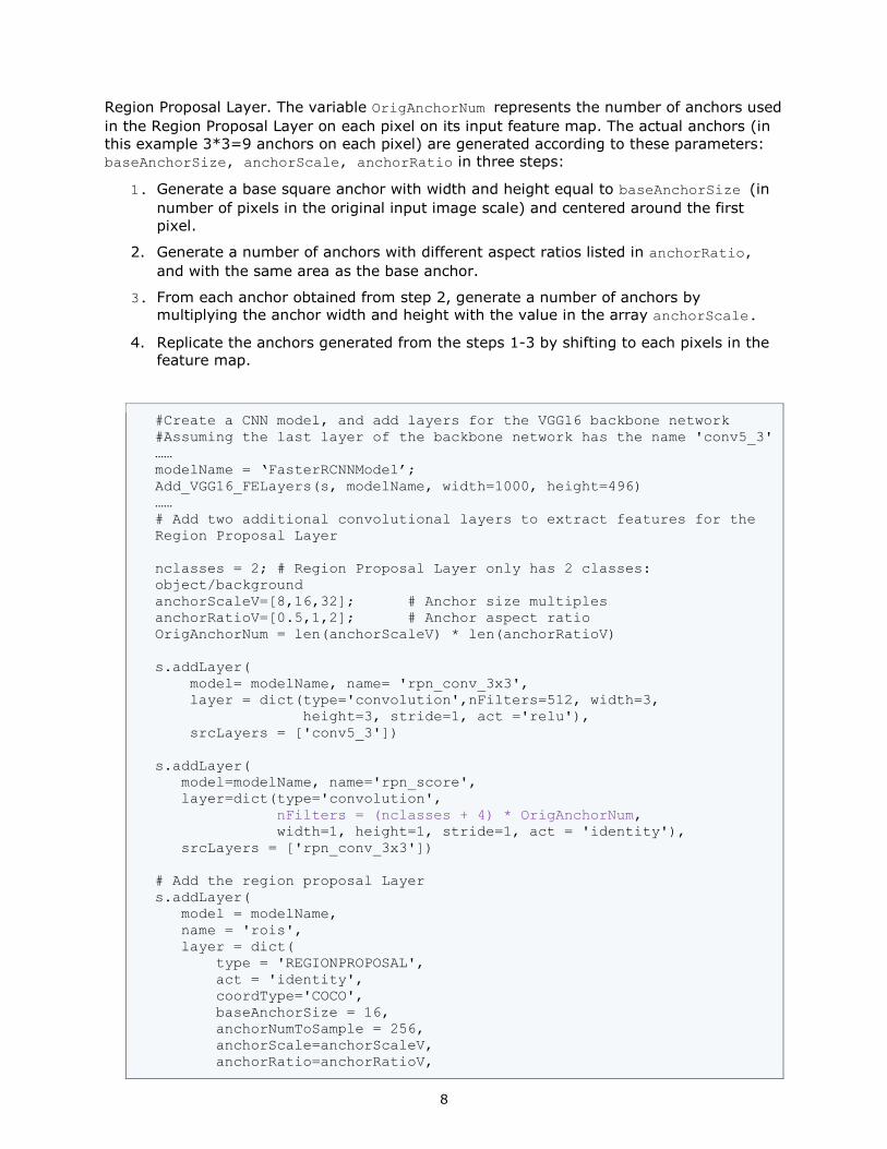
Region Proposal Layer. The variable OrigAnchorNum represents the number of anchors used
in the Region Proposal Layer on each pixel on its input feature map. The actual anchors (in
this example 3*3=9 anchors on each pixel) are generated according to these parameters:
baseAnchorSize, anchorScale, anchorRatio in three steps:
1. Generate a base square anchor with width and height equal to baseAnchorSize (in
number of pixels in the original input image scale) and centered around the first
pixel.
2. Generate a number of anchors with different aspect ratios listed in anchorRatio,
and with the same area as the base anchor.
3. From each anchor obtained from step 2, generate a number of anchors by
multiplying the anchor width and height with the value in the array anchorScale.
4. Replicate the anchors generated from the steps 1-3 by shifting to each pixels in the
feature map.
#Create a CNN model, and add layers for the VGG16 backbone network
#Assuming the last layer of the backbone network has the name 'conv5_3'
……
modelName = ‘FasterRCNNModel’;
Add_VGG16_FELayers(s, modelName, width=1000, height=496)
……
# Add two additional convolutional layers to extract features for the
Region Proposal Layer
nclasses = 2; # Region Proposal Layer only has 2 classes:
object/background
anchorScaleV=[8,16,32]; # Anchor size multiples
anchorRatioV=[0.5,1,2]; # Anchor aspect ratio
OrigAnchorNum = len(anchorScaleV) * len(anchorRatioV)
s.addLayer(
model= modelName, name= 'rpn_conv_3x3',
layer = dict(type='convolution',nFilters=512, width=3,
height=3, stride=1, act ='relu'),
srcLayers = ['conv5_3'])
s.addLayer(
model=modelName, name='rpn_score',
layer=dict(type='convolution',
nFilters = (nclasses + 4) * OrigAnchorNum,
width=1, height=1, stride=1, act = 'identity'),
srcLayers = ['rpn_conv_3x3'])
# Add the region proposal Layer
s.addLayer(
model = modelName,
name = 'rois',
layer = dict(
type = 'REGIONPROPOSAL',
act = 'identity',
coordType='COCO',
baseAnchorSize = 16,
anchorNumToSample = 256,
anchorScale=anchorScaleV,
anchorRatio=anchorRatioV,

9
),
srcLayers = ['rpn_score']
)
Table 4 The Region Proposal Layer and its Feature Extraction Layers
In Table 5, the roipooling layer is added with two source layers:
• the conv5_3 layer, which is the last layer of the backbone network,
• the rois layer, which is the region proposal layer.
The order of two source layer defines their usage here.
After two additional fully connection (FC) layers, the output of cls_score layer is used to
provide data to the final FastRCNN layer for classification of the object in the RoI, and the
output of bbox_pred layer is used for object bounding box regression in the RoI. You can
see how the output size n of the FC layers is related with the number of object categories.
The last layer for this model is the FastRCNN layer, which has three source layers; they are
in order the FC layer with classification data, and FC layer with bounding box regression
data, and the Region Proposal layer.
classNum = 20; # Number of Object Categories in the Model
s.addLayer(model=modelName, name='pool5',
layer = dict(type='roipooling', poolWidth=7, poolHeight=7),
srcLayers = ['conv5_3', 'rois']
)
s.addLayer(model=modelName, name='fc6',
layer = dict(type='fullconnect', n=4096, act='relu'),
srcLayers = ['pool5'])
s.addLayer(modelName, name='fc7',
layer = dict(type='fullconnect', n=4096, act='relu'),
srcLayers = ['fc6'])
s.addLayer(modelName, name='cls_score',
layer = dict(type='fullconnect', n=(classNum+1), act=’identity’),
srcLayers = ['fc7'])
s.addLayer(modelName, name='bbox_pred',
layer = dict(type='fullconnect',
n=4*(classNum+1), # The +1 is for the background category
act='identity'), srcLayers = ['fc7'])
s.addLayer(
model = modelName,
name = 'fastrcnn',
layer = dict(
type = 'fastrcnn',
nmsIouThreshold = 0.3,
detectionThreshold = 0.8
),
srcLayers = ['cls_score', 'bbox_pred', 'rois'])
Table 5 The ROI (Region of Interest) Pooling Layers, and FastRCNN Layers
TRAIN THE MODEL
After you prepared the images, the labeled data, and defined the model DAG as shown in
the previous sections, you can now start to train the object detector. Here we use a tiny
YOLO detector to show the process.
10
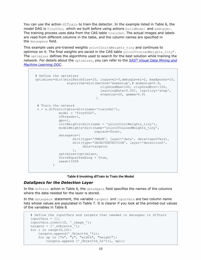
You can use the action dlTrain to train the detector. In the example listed in Table 6, the
model DAG is TinyYOLO, which we built before using actions buildModel and addLayer.
The training process uses data from the CAS table trainSet. The actual images and labels
are read from different columns in the table, and the column names are specified in
the dataspecs field.
This example uses pre-trained weights yolov2InitdWeights_tiny and continues to
optimize on it. The final weights are saved in the CAS table yolov2TrainedWeights_tiny".
The optimizer defines the algorithms used to search for the best solution while training the
network. For details about the optimizer, you can refer to the SAS® Visual Data Mining and
Machine Learning DOC.
# Define the optimizer
optimizer=dict(miniBatchSize=10, logLevel=3,debugLevel=2, maxEpochs=10,
algorithm=dict(method='momentum',# momentum=0.9,
clipGradMax=100, clipGradMin=-100,
learningRate=0.001, lrpolicy='step',
stepsize=20, gamma=0.9)
)
# Train the network
r = s.dlTrain(table=dict(name='trainSet'),
model = 'TinyYOLO',
nThreads=1,
gpu=1,
initWeights=dict(name = 'yolov2InitWeights_tiny'),
modelWeights=dict(name='yolov2TrainedWeights_tiny',
replace=True),
dataspecs=[
dict(type='IMAGE', layer='data', data=inputVars),
dict(type='OBJECTDETECTION', layer='detection0',
data=targets)
],
optimizer=optimizer,
forceEqualPadding = True,
seed=13308
)
Table 6 Invoking dlTrain to Train the Model
DataSpecs for the Detection Layer
In the dlTrain action in Table 6, the dataSpecs field specifies the names of the columns
where the data needed for the layer is stored.
In the dataspecs statement, the variable targets and inputVars are two column name
lists whose values are populated in Table 7. It is clearer if you look at the printed-out values
of the variables in Table 8.
# Define the inputVars and targets that needed in dataspec in dlTrain
inputVars = [];
inputVars.insert(0, '_image_');
targets = ['_nObjects_'];
for i in range(0,10):
targets.append('_Object%d_'%i);
for sp in ["x", "y", "width", "height"]:
targets.append ('_Object%d_%s'%(i, sp));

11
print ("targets")
print (targets);
print ("inputVars");
print (inputVars);
Table 7 Code to Generate the Variables Used in Dataspec
targets
['_nObjects_', '_Object0_', '_Object0_x', '_Object0_y', '_Object0_width',
'_Object0_height', '_Object1_', '_Object1_x', '_Object1_y',
'_Object1_width', '_Object1_height', '_Object2_', '_Object2_x',
'_Object2_y', '_Object2_width', '_Object2_height', '_Object3_',
'_Object3_x', '_Object3_y', '_Object3_width', '_Object3_height',
'_Object4_', '_Object4_x', '_Object4_y', '_Object4_width',
'_Object4_height', '_Object5_', '_Object5_x', '_Object5_y',
'_Object5_width', '_Object5_height', '_Object6_', '_Object6_x',
'_Object6_y', '_Object6_width', '_Object6_height', '_Object7_',
'_Object7_x', '_Object7_y', '_Object7_width', '_Object7_height',
'_Object8_', '_Object8_x', '_Object8_y', '_Object8_width',
'_Object8_height', '_Object9_', '_Object9_x', '_Object9_y',
'_Object9_width', '_Object9_height', '_Object10_', '_Object10_x',
'_Object10_y', '_Object10_width', '_Object10_height']
inputVars
['_image_']
Table 8 Output of the Print Statement: Values of the Dataspec Variables
Inside the dataSpecs statement in Table 6, the statement:
dict(type='IMAGE', layer='data', data=inputVars)
tells the training process that the input layer named data uses image data, and the name
of the column containing the image is represented by the variable inputVars, which in this
case means the image data needed is in the column _image_ in the input CAS table
trainSet.
The statement
dict(type='OBJECTDETECTION', layer='detection0', data=targets)
tells that the detection layer (with name detection0) uses data of type OBJECTDETECTION,
which consists of a set of columns in the input table.
Data type OBJECTDETECTION defines the meaning of each field in the list targets as
following:
• The number of labeled objects for each image is stored in a column whose name is
given in the first string item in the list targets, in this example, in the column
named _nObjects_;
• Each labeled object in the image uses five columns, whose names are in five
consecutive items in the list, for example, in the column with names _Object0_, _Object0_x, _Object0_y, _Object0_width, _Object0_height
• The order, not the name, of the five consecutive items, determines the usage of the
columns. Specifically, the first item points to the column for the object category,
and the 2-5 items, if in YOLO format, points to the columns for the x, y position,

12
and width and height of the object bounding box in order respectively.
Monitoring the Training Process
Table 9 shows some information you can see in the training process. The Fit Error currently
is calculated as an average of the value 1-IOU (Intersection over Union) for all images;
the IOU for each image is the average IOU for all the labeled object v.s. best matching
prediction pairs in the image, regardless of whether the prediction is selected as one of the
final detections or not.
WARNING: Only 1 out of 2 available GPU devices are used.
NOTE: The Synchronous mode is enabled.
NOTE: The total number of parameters is 15861648.
NOTE: The approximate memory cost is 357.00 MB.
NOTE: Loading weights cost 0.00 (s).
NOTE: Initializing each layer cost 1.47 (s).
NOTE: The total number of threads on each worker is 1.
NOTE: The total minibatch size per thread on each worker is 10.
NOTE: The maximum minibatch size across all workers for the synchronous
mode is 10.
NOTE: Epoch Learning Rate Loss Fit Error Time (s)
NOTE: 0 0.001 44.367 0.7135 0.41
NOTE: 1 0.001 16.287 0.6829 0.40
NOTE: 2 0.001 10.311 0.6061 0.39
NOTE: 3 0.001 7.0372 0.542 0.40
NOTE: 4 0.001 6.2692 0.4923 0.39
NOTE: 5 0.001 5.3297 0.4786 0.39
NOTE: 6 0.001 5.1382 0.4639 0.40
NOTE: 7 0.001 4.9569 0.4291 0.41
NOTE: 8 0.001 4.5718 0.3865 0.40
NOTE: 9 0.001 4.3239 0.3875 0.40
NOTE: The optimization reached the maximum number of epochs.
NOTE: The total time is 3.99 (s).
Table 9 Monitoring the Training Process
It is an art to train a deep neural network. For object detection network like this, you can
use pretrained weights that are trained on general publicly available classification data set
like IMAGENET, since they have a huge amount of data. After that, you can transfer the
weights into the detection network, and train it with your specific data set. When training a
new model, always start with a small sample of the data and try to overfit it.
The L2 Norm of the pre-trained weights should be small, otherwise, it is an indication that
the model lacks generalization capability. It is recommended to use L2 Norm and
randomMutation to prevent overfitting. If L2 Norm is set, the value should decrease and be
small during training.
During the detection network training, it is usually a good practice to start with a small
learning rate, and after a few epochs, increase the rate by 10~50 times.
SCORE USING TRAINED WEIGHTS
Scoring Using trained weights is similar with other deep learning tasks. In the following
scripts, the scoring results are saved in the CAS table detections.
s.dlscore(model='TinyYOLO',
initWeights='yolov2TrainedWeights_tiny',
table = 'scoringSet',
copyVars=['_path_', '_image_'],
13
nThreads=10,
miniBatchSize=1,
casout={'name':'detections', 'replace':True}
)
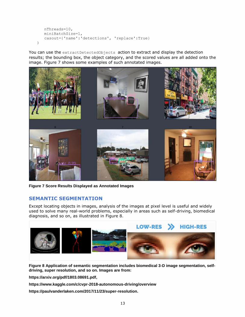
You can use the extractDetectedObjects action to extract and display the detection
results; the bounding box, the object category, and the scored values are all added onto the
image. Figure 7 shows some examples of such annotated images.
Figure 7 Score Results Displayed as Annotated Images
SEMANTIC SEGMENTATION
Except locating objects in images, analysis of the images at pixel level is useful and widely
used to solve many real-world problems, especially in areas such as self-driving, biomedical
diagnosis, and so on, as illustrated in Figure 8.
Figure 8 Application of semantic segmentation includes biomedical 3-D image segmentation, self-driving, super resolution, and so on. Images are from:
https://arxiv.org/pdf/1803.08691.pdf,
https://www.kaggle.com/c/cvpr-2018-autonomous-driving/overview
https://paulvanderlaken.com/2017/11/23/super-resolution.

14
Image semantic segmentation is one of the techniques to understand an image at pixel
level. Specifically, it attempts to partition the image into semantically meaningful parts, and
to classify each part into one of the pre-defined classes. That is, each pixel in the image is
assigned to an object class as shown in Figure 9.
Figure 9 An example of semantic segmentation. One of the four pre-defined labels is given to each pixel in the image to show the boundaries and shape of each object. Image is from https://www.analyticsvidhya.com/blog/2017/11/heart-sound-segmentation-deep-learning.
There are many promising semantic segmentation models, including FCN [9], U-Net [10],
SegNet [11], and DeepLab [12]. This paper focuses on U-Net model, which consists of an
encoding path to capture context, and a symmetric decoding path that enables pixelwise
prediction. This paper also introduces the semantic segmentation feature in SAS Deep
Learning through a practical example.
MODEL SPECIFICATION
Fully connected (FC) layers connect every neuron in one layer to every neuron in another
layer and are widely used in traditional neural networks to flatten the matrices and to
classify the images. However, it fixes the dimension and throws away the spatial structure
of the layers. Since for semantic segmentation the inference is at pixel level, it is crucial to
maintain the dimensional structure, and naturally the FC layers are replaced by fully
convolutional layers.
Based on this idea, the U-Net model contains two parts: the down-sampling encoding part,
including convolution layers and pooling layers, that gradually reduces the spatial dimension
of the input images, and the up-sampling decoding part, including convolution layers and
transpose convolution layers, the recovers the object details. In order to inherit localization
information from the encoding process, concatenation layers are also used in the model, as
shown in Figure 10. This model is named after its U-shape, as the encoding part and
decoding part are symmetric. Starting from the bottleneck layer, which in this case is the
8*8*1024 layer at the bottom of the U-shape, the up-sampling process is the reversed
image of the down-sampling process, with pooling layers replaced by transpose convolution
layers.

15
Figure 10 U-Net architecture. The input layer contains 256*256 color images. The resolution of bottleneck layer is 8*8. Each blue box is a feature map of denoted size.
GROUND TRUTH FORMAT
Both image and wide format data are supported in the segmentation model. If using the
wide format, each column represents the value of one pixel of the input image. Specifically,
the first column gives the class label of the top left pixel (0, 0), the second column
represents the second pixel (0, 1). The column for the last pixel in the first row of the image
is followed by that of the first pixel in the second row (1, 0) of the image. The last column
gives the class of the bottom right pixel of the image. The values could be either numeric
(0, 1, 2, …) or categorical (people, car, background, …).
If using image type ground truth for pixel-wise classification, then the pixel values should be
an integer no more than the number of classes. For example, if there are four different
classes in the image, then each pixel of the ground truth should be a number in [0, 1, 2, 3].
SOCCER PLAYER DATA SET
The data set contains 170 256*256 color images and annotations as shown in Figure 11.
They are divided into three parts: training (70%), validation (20%) and testing (10%).
Figure 11 The data set contains 170 color images and annotations. Three classes are pre-defined: soccer player, ball, and background.

16
Image type ground truth is used for this data set as in Figure 12. Specifically, the data
would contain two columns of images, _image_ and _labels_. The first is the input, which
contains images of 256*256*3 taking values between [0, 255]. The second is the ground
truth, which are 256*256*1 images taking values in [0, 1, 2], representing their three
classes: soccer player, ball, and background.
Figure 12 Columns in the data set.
BUILDING MODEL DAG
The model DAG is built using DLPy, an open-source, high-level Python package for deep
learning. An example of the syntax is given below.
Inputs = InputLayer(3, 256, 256, scale = 1.0 / 255,
random_mutation='random', name='InputLayer_1')
conv1 = Conv2d(64, 3, act = 'identity', init=init)(inputs)
bn1 = BN(act = 'relu')(conv1)
conv1 = Conv2d(64, 3, act = 'identity', init=init)(bn1)
bn1 = BN(act = 'relu')(conv1)
pool1 = Pooling(2)(bn1)
……
tconv7 = Transconvo(1024, 3, stride = 2, act='relu', padding = 1,
output_size = (16, 16, 1024), init=init)(bn6)
merge7 = Concat(src_layers = [bn5, tconv7])
conv7 = Conv2d(1024, 3, act = 'identity', init=init)(merge7)
bn7 = BN(act = 'relu')(conv7)
conv7 = Conv2d(1024, 3, act = 'identity', init=init)(bn7)
bn7 = BN(act = 'relu')(conv7)
……
conv12 = Conv2d(3, 3, act = ‘relu’, init=init)(bn11)
seg1 = Segmentation(name='Segmentation_1', act=’softmax’,
error=’entropy’)
Since the tensor dimension of the segmentation layer is entirely inherited from its source
layer, the feature map size of its source layer should be equal to that of the ground truth,
while the number of channels should be equal to the number of classes. In this case, the
output size of layer conv12 is 256*256*3. The default activation function is softmax and
the default error type is cross-entropy.
TRAINING AND SCORING
The model is trained using ADAM algorithm for 60 epochs, with mini-batch size = 10 and
number of threads = 1. Sample code for training is as below. Part of the training process is
shown in Figure 13.
Inputs = InputLayer(3, 256, 256, scale = 1.0 / 255,
random_mutation='random', name='InputLayer_1')
dataspecs=[dict(type='image', layer='InputLayer_1', data=['_image_']),

17
dict(type='image', layer='Segmentation_1', data=['labels'])]
optimizer = dict(miniBatchSize=10, regL2=0.0005,
algorithm=dict(method="adam", lr=2e-4, lrPolicy='step',
gamma=0.9, stepSize=10),
maxEpochs=60, logLevel=2)
s.dlTrain(model=model_name, table=train, validtable=valid, nthreads=1,
modelWeights = dict(name = 'seg_weights', replace = True),
dataspecs=dataspecs,
optimizer = optimizer)
Figure 13 Part of the training process
The loss error is the sum of cross-entropy of all pixels, while the fit error is the
misclassification rate averaged on all pixels. Both errors are supposed to decrease during
training process, as indicated in Figure 13.
For segmentation models, dataspecs must be specified for input layers and segmentation
layers to define the data types and columns. In this example, images are used for both
input and segmentation layers.
The following code is for scoring on the testing data. The testing output is also given below
in Figure 14. For each image, the output table contains the pixel-wise prediction, along with
the predicted probability. For example, the first pixel is assigned label 0 with probability
higher than 0.99, as shown in columns _DL_PredName0_ and _DL_PredP0_. Visualization of
the scoring results can be easily achieved based on the output tables.
s.dlscore(modeltable=model_name, initweights='seg_weights', table=test,
nthreads=1, casout=dict(name='output', replace=True))

18
Figure 14 Scoring output on testing data.
The scoring mis-classification rate on the testing data is 0.76%, which means out of 65,536
pixels in each image, only less than 500 pixels are miss-labeled. Some of the scoring
visualization results are given in Figure 15.
Figure 15 Scoring results visualization. The raw images are shown in the first column, followed by ground truth annotation in the second column. The third column contains predictions.

19
CONCLUSION
SAS has extended its deep learning toolkit to support object detection and semantic
segmentation in its recent release. This new functionality is available through CAS action
sets in SAS Visual Data Mining and Machine Learning, as well as in the DLPy open-source
project.
With the new extension, SAS deep learning empowers customers to build an end to end
solutions to computer vision problems involving tasks of image classification, keypoint
detection, object detection, and semantic segmentation.
Specific examples demonstrate how some new layers, when combined with other deep
learning, image processing action sets, enable customers to load, explore the data, build the
model architecture, train the network, perform the inference, and visualize the results.
Development efforts involving instance segmentation is in progress and will be available to
customers in the future.
REFERENCES
[1] J. Redmon and A. Farhadi, "YOLO9000: Better, Faster, Stronger," in IEEE Conference on
Computer Vision and Pattern Recognition (CVPR), Honolulu, HI, USA, 2017.
[2] W. Liu, D. Anguelov, D. Erhan, C. Szegedy, S. Reed, C.-Y. Fu and A. C. Berg, "SSD:
Single shot multibox detector," in Proceedings of the European Conference on Computer
Vision , 2016.
[3] S. Ren, K. He, R. Girshick and J. Sun, "Faster R-CNN: Towards Real-Time Object
Detection with Region Proposal Networks," IEEE Transactions on Pattern Analysis and
Machine Intelligence, vol. 39, no. 6, pp. 1137-1149, 1 June 2017.
[4] T. Lin, P. Goyal, R. Girshick, K. He and P. Dollár, "Focal Loss for Dense Object
Detection," in IEEE International Conference on Computer Vision, Venice, 2017.
[5] J. Dai, Y. Li, K. He and J. Sun, "R-FCN: Object Detection via Region-based Fully
Convolutional Networks," in Neural Information Processing Systems Conference, 2016.
[6] T.-Y. Lin, P. Dollár, R. Girshick, K. He, B. Hariharan and S. Belongie, "Feature Pyramid
Networks for Object Detection," in The IEEE Conference on Computer Vision and Pattern
Recognition (CVPR), 2017.
[7] R. Girshick, J. Donahue, T. Darrell and J. Malik, "Rich Feature Hierarchies for Accurate
Object Detection and Semantic Segmentation," in IEEE Conference on Computer Vision
and Pattern Recognition, Columbus, OH, 2014.
[8] R. Girshick, "Fast R-CNN," in Proc. IEEE Int. Conf. Comput. Vis., 2015.
[9] J. E. S. a. T. D. Long, "Fully convolutional networks for semantic segmentation," In
Proceedings of the IEEE conference on computer vision and pattern recognition, pp. pp.
3431-3440, 2015.
[10] O. P. F. a. T. B. Ronneberger, "U-net: Convolutional networks for biomedical image
segmentation," International Conference on Medical image computing and computer-
assisted intervention, pp. pp. 234-241, 2015.
[11] V. K. A. &. C. R. Badrinarayanan, "Segnet: A deep convolutional encoder-decoder
architecture for image segmentation," IEEE transactions on pattern analysis and machine
intelligence, 39(12), 2481-2495., 2017.

20
[12] L.-C. G. P. I. K. K. M. a. A. L. Y. Chen, "Deeplab: Semantic image segmentation with
deep convolutional nets, atrous convolution, and fully connected crfs," IEEE transactions
on pattern analysis and machine intelligence, 40(4), 834-848., 2018.
[13] V. a. F. V. Dumoulin, "A guide to convolution arithmetic for deep learning," arXiv preprint
arXiv:1603.07285 (2016)..
RECOMMENDED READING
• SAS® Visual Data Mining and Machine Learning DOC, available at
http://support.sas.com/software/products/visual-data-mining-machine-
learning/index.html#s1=2
• DLPy - SAS Viya Deep Learning API for Python, available at
https://github.com/sassoftware/python-dlpy
CONTACT INFORMATION
Your comments and questions are valued and encouraged. Contact the authors at:
Xindian Long
SAS Institute
+1 919-531-2594
Maggie Du
SAS Institute
+1 919-531-5291
Xiangqian Hu
SAS Institute
+1 919-531-1423
SAS and all other SAS Institute Inc. product or service names are registered trademarks or trademarks of SAS Institute Inc. in the USA and other countries. ® indicates USA registration.