exploration of the three-player partizan game of
TRANSCRIPT
EXPLORATION OF THE THREE-PLAYER PARTIZAN GAME OFRHOMBINATION
BY
KATHERINE A. GREENE
A Thesis Submitted to the Graduate Faculty of
WAKE FOREST UNIVERSITY GRADUATE SCHOOL OF ARTS AND SCIENCES
in Partial Fulfillment of the Requirements
for the Degree of
MASTER OF ARTS
Mathematics and Statistics
May 2017
Winston-Salem, North Carolina
Approved By:
Sarah K. Mason, Ph.D., Advisor
Edward E. Allen, Ph.D., Chair
R. Jason Parsley, Ph.D.

Acknowledgments
I owe my thanks to many for helping me get where I am today.
Firstly, I’m grateful to God for His guidance, abundant blessings, answers toprayer, and peace in my life and education.
I’d like to thank my advisor, Dr. Sarah Mason, for all her help on this thesis andguiding me the whole way. She has been both a mentor and a friend throughout mystay at Wake Forest.
I’m so thankful to my boyfriend, Max, for his constant love and support. Heis always such a source of strength and motivation to me, providing the calminginfluence that often sparks my mathematical creativity.
A special thanks goes to my family for their great support, especially my motherfor teaching me to love math and bringing me to this program. I greatly appreciatemy grandparents and all they’ve done in taking care of me and supporting me in mywork and education.
Thanks goes to Dr. Allen, for transitively bringing me here. I appreciate all myprofessors I’ve had at Wake: Dr. Gaddis, Dr. Robinson, Dr. Howards, Dr. Hepler,Dr. Rouse, and especially Dr. Parsley.
Lastly, I’m thankful for my classmates, especially Brad Hall, who never fails tomake me laugh, making awesome math jokes and coming up with fun math satires.Also thanks goes to Richard Harris and my office mates, Curtis Clark and LelandKent, for being supportive and encouraging friends.
ii

Table of Contents
Acknowledgments . . . . . . . . . . . . . . . . . . . . . . . . . . . . . . . . . . . . . . . . . . . . . . . . . . . . . . . . . . . . . . ii
List of Figures . . . . . . . . . . . . . . . . . . . . . . . . . . . . . . . . . . . . . . . . . . . . . . . . . . . . . . . . . . . . . . . . . iv
List of Tables . . . . . . . . . . . . . . . . . . . . . . . . . . . . . . . . . . . . . . . . . . . . . . . . . . . . . . . . . . . . . . . . . . v
Abstract . . . . . . . . . . . . . . . . . . . . . . . . . . . . . . . . . . . . . . . . . . . . . . . . . . . . . . . . . . . . . . . . . . . . . . . vi
Chapter 1 Introduction to Combinatorial Game Theory . . . . . . . . . . . . . . . . . . . . . . 1
1.1 Two-Player Games . . . . . . . . . . . . . . . . . . . . . . . . . . . . 1
1.2 Three-Player Games . . . . . . . . . . . . . . . . . . . . . . . . . . . 12
Chapter 2 Rhombination . . . . . . . . . . . . . . . . . . . . . . . . . . . . . . . . . . . . . . . . . . . . . . . . . . . . . 16
Chapter 3 Comparisons, Posets, and Symmetry . . . . . . . . . . . . . . . . . . . . . . . . . . . . . . 24
3.1 Cincotti’s Approach to Partial Order . . . . . . . . . . . . . . . . . . 24
3.2 Our Approach . . . . . . . . . . . . . . . . . . . . . . . . . . . . . . . 25
3.3 Rotations and Reflections . . . . . . . . . . . . . . . . . . . . . . . . 28
Chapter 4 Future Directions . . . . . . . . . . . . . . . . . . . . . . . . . . . . . . . . . . . . . . . . . . . . . . . . . 33
4.1 Additional Concepts to Prove . . . . . . . . . . . . . . . . . . . . . . 33
4.2 Number Games . . . . . . . . . . . . . . . . . . . . . . . . . . . . . . 36
Bibliography . . . . . . . . . . . . . . . . . . . . . . . . . . . . . . . . . . . . . . . . . . . . . . . . . . . . . . . . . . . . . . . . . . . 40
Appendix A Rhombination Positions for the Outcome Classes. . . . . . . . . . . . . . . . . 41
Appendix B Sample Game Trees for Rhombination . . . . . . . . . . . . . . . . . . . . . . . . . . . 42
Curriculum Vitae Katie Greene . . . . . . . . . . . . . . . . . . . . . . . . . . . . . . . . . . . . . . . . . . . . 44
iii

List of Figures
1.1 Two-Player Game Tree . . . . . . . . . . . . . . . . . . . . . . . . . . 4
1.2 Poset Chart Example . . . . . . . . . . . . . . . . . . . . . . . . . . . 9
1.3 Game Tree Trimming . . . . . . . . . . . . . . . . . . . . . . . . . . . 11
3.1 The Posets of 1L, 1C , 1R, and 0 . . . . . . . . . . . . . . . . . . . . . . 27
iv
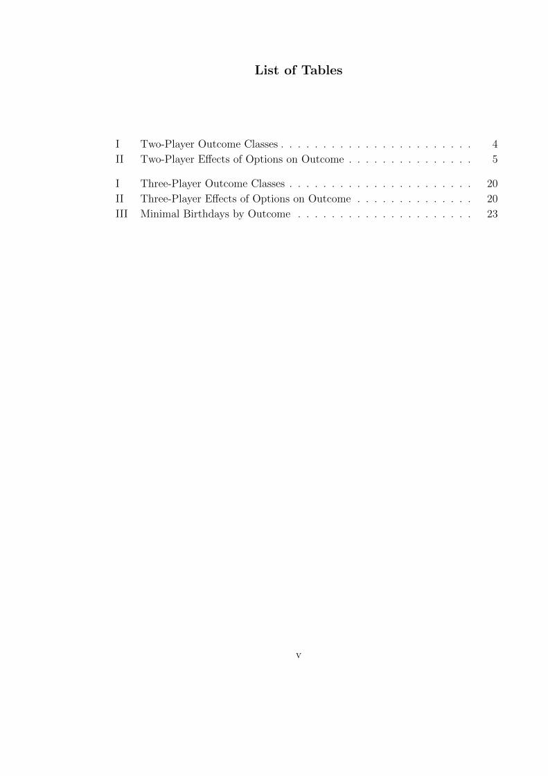
List of Tables
I Two-Player Outcome Classes . . . . . . . . . . . . . . . . . . . . . . . 4
II Two-Player Effects of Options on Outcome . . . . . . . . . . . . . . . 5
I Three-Player Outcome Classes . . . . . . . . . . . . . . . . . . . . . . 20
II Three-Player Effects of Options on Outcome . . . . . . . . . . . . . . 20
III Minimal Birthdays by Outcome . . . . . . . . . . . . . . . . . . . . . 23
v

Abstract
We introduce a new combinatorial three-player partizan game called Rhombinationand expand some ideas from two-player game theory into three-player game theory.
Cincotti’s three-dimensional Domineering is distinct from Rhombination. We provethe Fundamental Theorem for three-player games, given the player preference set byLi. We set a bound on the number of games born on day n. Comparisons are madewith Cincotti’s partial ordering and a generalization of two-player partial order isdefined for three-player games. We make observations on outcome classes of gamesand find effects of rotation and reflection on outcome. We give many ideas for futuretheorems to prove or directions to take, including a potential method for definingthree-player number games.
vi
Chapter 1: Introduction to Combinatorial Game Theory
Who will win? How do we win? This is what we all ask when we play a game
of any sort. In combinatorial game theory, we develop methods to find the optimal
strategies and winners of given game positions.
1.1 Two-Player Games
We begin with two-player games, for which much of the following is standard. See
[1] for details on two-player game theorems and for references on the given two-
player games. In this section, all games are between two players. We begin by
defining combinatorial games. There are two players, called Left (Player 1) and
Right (Player 2), who take turns alternating moves until one no longer can play.
Combinatorial games do not involve chance, meaning there is no random element
such as dice rolling or card shuffling. These games have perfect information, meaning
both players can see all possible moves. Combinatorial games must have a finite
number of moves, contain no loops leading to previous positions, and under normal
play the last player to move wins.
A game is partizan when different players cannot necessarily make the same
moves and an impartial game is one in which the options are the same for each
player. We will be considering partizan games.
Examples of combinatorial games include Nim, Subtraction(L|R), Amazons, Clob-
ber, Hackenbush, Push/Shove, and Toppling Dominoes. See [1] for descriptions.
Subtraction(L|R) is a game in which we have a pile of counters and each player
is given certain amounts they can remove. For example, Subtraction(1,4|2,3) means
that Left can take either 1 or 4 counters out of the pile on their turn and Right may
1

take either 2 or 3 on their turn. An example game sequence would be: 16→L 15→R
12→L 11→R 8→L 7→R 5→L 1 now Right cannot move, so Left wins.
The following are common games that do not quite fit all the requirements for
combinatorial games, but can be analyzed similarly.
• In Dots and Boxes, players do not always alternate as they get an extra move
when they bound a box.
• Battleship does not have perfect information, as the players cannot see both
boards.
• Chess contains draws, so there is not always a winner.
• Go determines the winner by who has the most pieces rather than who goes
last.
• Chomp is a combinatorial game, but since the last player to move loses, it is
not normal play, but misere play.
Some games that do not satisfy two or more of the requirements for combinatorial
games are Poker, Risk, Monopoly, Blackbox, Scrabble, etc. These games are far from
combinatorial games as some have chance, multiple players, imperfect information,
and determine the winners in different ways.
We will use the game Domineering for our two-player examples, defined as
follows. We start with a board of squares in which players take turns placing 2x1
domino tiles on the board with no overlap in the tiles. Left can only place dominos
oriented vertically and Right can only place dominos oriented horizontally.
A game G is classified by a set of game options. Left has a set of possible
moves, denoted GL, and Right has a set of possible moves, denoted GR, so the game
G = {GL|GR}. The zero game is the game with no options: 0 = {|}.
2
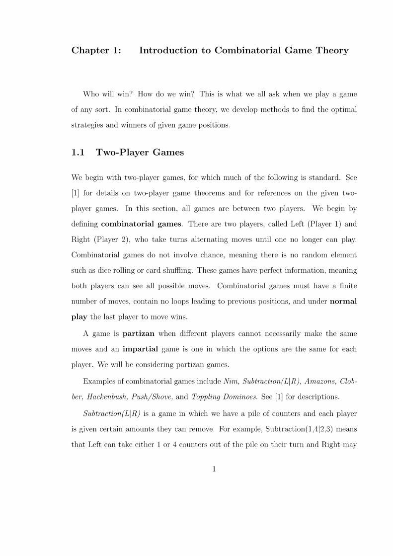
Example: Let G = . Then G = { , | , }. Notice here that once
a section of the board is covered with a tile, it is the same as the position with the
covered squares removed, so G = { , | , }. Since we have duplicate options
here, and a player will choose only one, we can ignore the extra copies and G = { |
}. Because = {0|} and = {|0}, we have G = {{0|}|{|0}}. These collections
of sets within sets can be confusing though, so when showing the sets of game options
within games, we use double bars to separate the options in the superset and single
bars to separate the options in the subsets. Thus G = {{0|∅}|{∅|0}} can be written
as G = {0|∅||∅|0}.
Notice that some moves in which we remove the squares covered by tiles will leave
disconnected squares. These isolated squares can be ignored since no moves can be
made on them. They are of no consequence to the game position.
Example: = = .
We can create what we call a game tree which charts all the possible moves
throughout the game. For full game trees, we include both Left and Right options
because games can be subsets of other games and so we may move on a game in an
order that is not the given player order. Two games, G and H, are called isomorphic,
denoted by G ∼= H, if their game trees are the same. If we have two options for a
player that are isomorphic, we only need to consider one of those options, so if GL =
{ , }, since ∼= , then GL = { }.
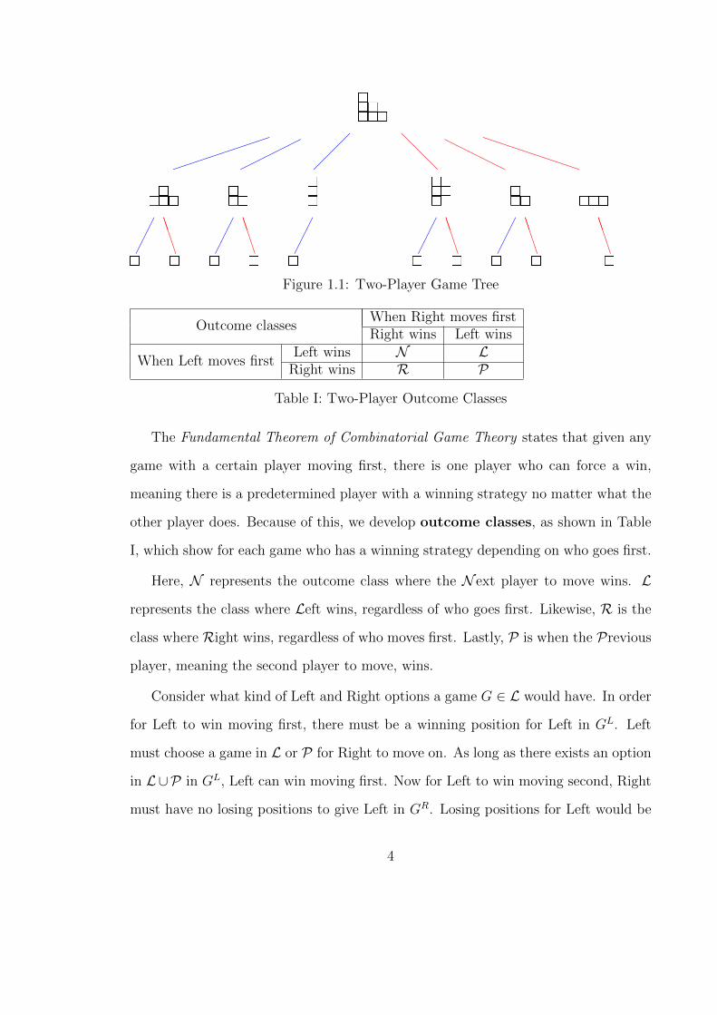
Example: The game tree for = { , , | , , } is displayed
in Figure 1.1.
The solitary boxes on the leaves of the game tree represent 0 games, which are
where the game sequences end since there are no more possible moves for either player.
3
����
����
���
��
���
@@
@
HHH
HH
PPPP
PPPP
���
BBBB
���
BBBB
���
���
BBBB
���
BBBB
BBBB
Figure 1.1: Two-Player Game Tree
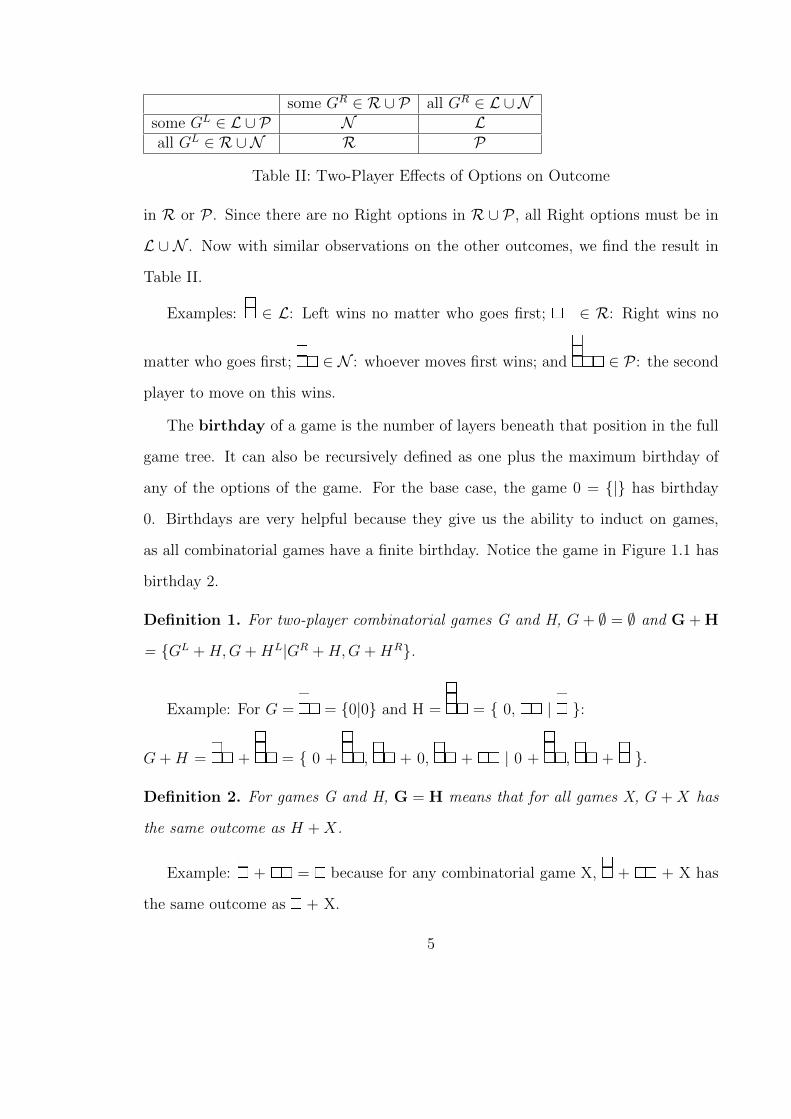
Outcome classesWhen Right moves firstRight wins Left wins
When Left moves firstLeft wins N L
Right wins R P
Table I: Two-Player Outcome Classes
The Fundamental Theorem of Combinatorial Game Theory states that given any
game with a certain player moving first, there is one player who can force a win,
meaning there is a predetermined player with a winning strategy no matter what the
other player does. Because of this, we develop outcome classes, as shown in Table
I, which show for each game who has a winning strategy depending on who goes first.
Here, N represents the outcome class where the N ext player to move wins. L
represents the class where Left wins, regardless of who goes first. Likewise, R is the
class where Right wins, regardless of who moves first. Lastly, P is when the Previous
player, meaning the second player to move, wins.
Consider what kind of Left and Right options a game G ∈ L would have. In order
for Left to win moving first, there must be a winning position for Left in GL. Left
must choose a game in L or P for Right to move on. As long as there exists an option
in L∪P in GL, Left can win moving first. Now for Left to win moving second, Right
must have no losing positions to give Left in GR. Losing positions for Left would be
4
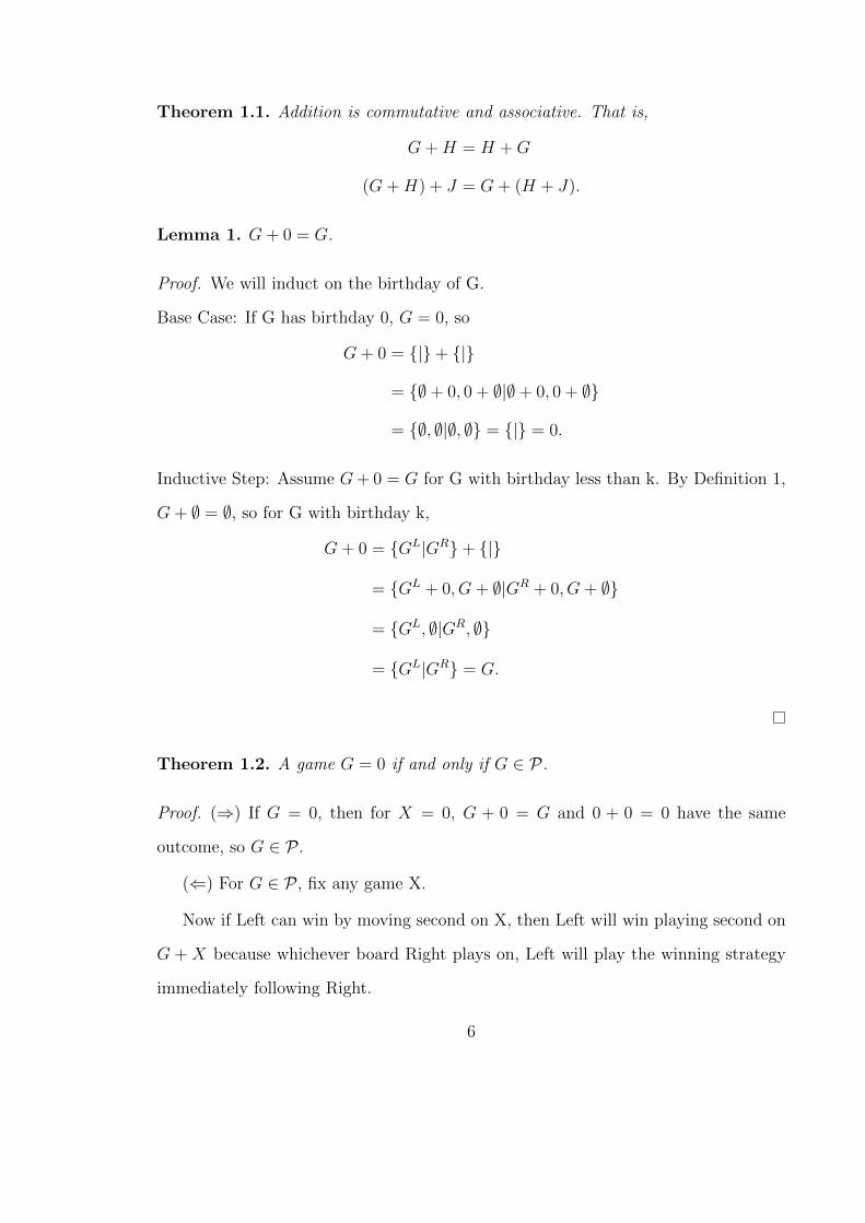
some GR ∈ R ∪ P all GR ∈ L ∪Nsome GL ∈ L ∪ P N Lall GL ∈ R ∪N R P
Table II: Two-Player Effects of Options on Outcome
in R or P . Since there are no Right options in R ∪ P , all Right options must be in
L ∪ N . Now with similar observations on the other outcomes, we find the result in
Table II.
Examples: ∈ L: Left wins no matter who goes first; ∈ R: Right wins no
matter who goes first; ∈ N : whoever moves first wins; and ∈ P : the second
player to move on this wins.
The birthday of a game is the number of layers beneath that position in the full
game tree. It can also be recursively defined as one plus the maximum birthday of
any of the options of the game. For the base case, the game 0 = {|} has birthday
0. Birthdays are very helpful because they give us the ability to induct on games,
as all combinatorial games have a finite birthday. Notice the game in Figure 1.1 has
birthday 2.
Definition 1. For two-player combinatorial games G and H, G+ ∅ = ∅ and G + H
= {GL +H,G+HL|GR +H,G+HR}.
Example: For G = = {0|0} and H = = { 0, | }:
G+H = + = { 0 + , + 0, + | 0 + , + }.
Definition 2. For games G and H, G = H means that for all games X, G + X has
the same outcome as H +X.
Example: + = because for any combinatorial game X, + + X has
the same outcome as + X.
5
Theorem 1.1. Addition is commutative and associative. That is,
G+H = H +G
(G+H) + J = G+ (H + J).
Lemma 1. G+ 0 = G.
Proof. We will induct on the birthday of G.
Base Case: If G has birthday 0, G = 0, so
G+ 0 = {|}+ {|}
= {∅+ 0, 0 + ∅|∅+ 0, 0 + ∅}
= {∅, ∅|∅, ∅} = {|} = 0.
Inductive Step: Assume G+ 0 = G for G with birthday less than k. By Definition 1,
G+ ∅ = ∅, so for G with birthday k,
G+ 0 = {GL|GR}+ {|}
= {GL + 0, G+ ∅|GR + 0, G+ ∅}
= {GL, ∅|GR, ∅}
= {GL|GR} = G.
Theorem 1.2. A game G = 0 if and only if G ∈ P.
Proof. (⇒) If G = 0, then for X = 0, G + 0 = G and 0 + 0 = 0 have the same
outcome, so G ∈ P .
(⇐) For G ∈ P , fix any game X.
Now if Left can win by moving second on X, then Left will win playing second on
G + X because whichever board Right plays on, Left will play the winning strategy
immediately following Right.
6

If Left can win moving first on X, then moving first on G+X, Left will play first
on X, then follow the previous player winning strategy moving on whichever board
Right moves on.
Symmetrically, if Right wins moving first or second on X, then they can use the
same strategy to make the same outcome on G + X. Thus G + X and 0 + X have
the same outcome and G = 0.
Now we have a set with a binary operation which is closed, associative, commu-
tative, and has identity. This leads us to look at the algebraic structure of games.
Definition 3. An abelian group is a set paired with a binary operation (S, ?) which
has the properties:
Closure: a ? b ∈ S, ∀a, b ∈ S,
Associativity: (a ? b) ? c = a ? (b ? c), ∀a, b, c ∈ S,
Identity: ∃e ∈ S 3 e ? a = a = a ? e, ∀a ∈ S,
Inverses: ∀a ∈ S,∃a−1 ∈ S 3 a ? a−1 = e = a−1 ? a,
and Commutativity: a ? b = b ? a, ∀a, b ∈ S.
Example: The integers under addition, (Z,+) form an abelian group. Closure,
associativity, and commutativity hold. Our identity is 0 and the inverse of any integer
a is −a.
Games form an abelian group under game addition. The identity game is 0 = {|}
and the inverse of game G is recursively given to be −G = {−GR| −GL}.
7

Example: The inverse of is:
− = −{0, | } = −{GL|GR}
= {− | − 0,− } = {−GR| −GL}
= { |0, } = .
Notice that this inverse is a reflection along the diagonal. It turns out in Domi-
neering that all game positions are inverses to their diagonal reflections.
Theorem 1.3. For any two-player combinatorial game G, G+ (−G) = 0.
Proof. We will induct on the birthday.
Base Case: G = 0, so 0 + (−0) = 0 + 0 = 0.
Assume this statement is true for games with birthday less than k. Let G have
birthday k.
If Left moves first, Left can move either on G or −G.
Case 1: Left moves on G; then we have GL + (−G), and to force a win, Right
will move on −G to give us the game GL + (−GL) which is 0 ∈ P by the inductive
hypothesis, so Right wins.
Case 2: Left moves on −G; then we have G + (−GR), and to force a win, Right
will move on G to give us the game GR + (−GR) which is 0 ∈ P by the inductive
hypothesis, so Right wins. The argument for Right moving first similarly has Left
win in all cases.
Since we proved that regardless what the first player does, the second player can
respond and force a win, we know the game is in P , so it must be equal to 0.
Definition 4. A partially ordered set, or poset, is a set paired with a partial
8

1
23
4
5
6
7
8
9 10
11
12
PPPP
PPPP
P
ZZZ
ZZ
�����
����
����
�
ZZ
ZZZ
ZZ
ZZZ
�����
ZZ
ZZZ
Figure 1.2: Poset Chart Example
ordering relation (S,≥) where the partial ordering relation is reflexive, antisymmetric,
and transitive.
Reflexive: For x ∈ S, x ≥ x.
Antisymmetric: For x, y ∈ S, if x ≥ y and y ≥ x, then x = y.
Transitive: For x, y, z ∈ S, if x ≥ y and y ≥ z, then x ≥ z.
Example: Consider the set {1, 2, 3, 4, 5, 6, 7, 8, 9, 10, 11, 12} with the ordering: m ≥
n iff n|m. This is a poset with Hasse Diagram [2] shown in Figure 1.2.
Definition 5. G ≥ H, means for all games X, Left wins G+X whenever Left wins
H +X.
Example: ≥ . For any game X, if Left wins X + , then Left will win X
+ because they play their winning strategy on X. Now Right has one less move, so
there is no disadvantage to Left.
Games form a partially ordered set under the relation in Definition 5. It is reflexive
because given game G, then for all X, if Left wins G + X then Left will win G + X,
so G ≥ G. It is antisymmetric because if G ≥ H and H ≥ G, then ∀X Left wins
H +X implies Left wins G+X and Left wins G+X implies Left wins H +X. Thus
9

G + X and H + X have the same outcome, so G = H. Transitivity follows because
if G ≥ H and H ≥ K, then ∀X Left wins K + X implies Left wins H + X which
implies Left wins G+X, so G ≥ K.
We can create what we call values of games, which are rational numbers that
measure how favorable the games are for each player. The games that can be assigned
a value are called number games. For any number game N , if N is negative, N ∈ R,
if N is positive, N ∈ L, and if N is 0, N ∈ P . No game in N can be a number game as
it is neither better for Left nor Right and is not equal to 0. This creates a well-ordered
subset of games in L,R, or P .
Example: is the number game 1 and is the number game -1. As we would
expect, + = 1− 1 = 0.
For the sake of future chapters, we will say ≥L is the same as ≥, since larger
numbers are better for Left and we will define ≥R to be the same as ≤, since smaller
numbers are better for Right.
With two-player games, we can also trim the game trees, creating an equivalent
game tree in reduced form, which is called canonical form. Given just two trim-
ming moves, we can cut down the game trees so that all games that are equal have
isomorphic game trees in canonical form.
We will glance over the three-player generalization for canonical form in Chapter
4. The following theorems are taken from [1].
Theorem 1.4. If G = {A,B,C, . . . |H, I, J, . . . } and B ≥L A, then G = G′ where
G′ = {B,C, . . . |H, I, J, . . . }.
Similarly for Right, if H ≥R I, then option I can be removed. Here options A and
I are called dominated options. The theorem allows us to remove these.
Theorem 1.5. Fix a game G = {A,B,C, . . . |H, I, J, . . . } and suppose that for
10

Game Tree Canonical Form
����
��
���
@@@
���
AAA
AAA
���
���
Figure 1.3: Game Tree Trimming
some Right option of A, call it AR, G ≥L AR. If we denote the Left options of
AR by {W,X, Y, . . . } then AR = {W,X, Y, . . . | . . . }, we can define the new game
G′ = {W,X, Y, . . . , B, C, . . . |H, I, J, . . . }, then G = G′.
For the situations in which the theorem applies, we say A is a reversible option,
meaning that the move reverses through A, so we can bypass it.
Example: Let G = = { 0, | }. Here, ∈ GL is both a dominated
option and a reversible option. The full game tree and canonical form are displayed
in Figure 1.3. Note that G ∈ L.
To show that is dominated, notice that 0 ≥L , so by Theorem 1.4, we have
G = { 0 | }.
To show that is also reversible, we notice that the Right option of is 0.
Since R = 0 ≤L G, by Theorem 1.5, we can substitute the Right options of
as a Left option, giving us G = { 0, 0 | }. Now we can remove the extra 0 by
isomorphic copies or by dominated options, giving us G = { 0 | }.
11

1.2 Three-Player Games
Three-player games require an additional player. We will call the new player Cen-
ter. There is no general convention for three-player partizan games, so we will be-
gin by looking at the research that has been done. In all cases, we play cyclically:
(L,C,R,L,C,R...). We define game options similarly to two-player games, adding
GC , the Center options of a game G = {GL|GC |GR}.
Cincotti introduces a three-dimensional Domineering game [3]. We will use it
for our examples. This game is played on a finite three-dimensional grid with edges
parallel to the x, y, and z axes, where players move by placing 2x1x1 dominoes. Left
places dominoes parallel to the z-axis, Center places dominoes parallel to the x-axis,
and Right places dominoes parallel to the y-axis. So = {0||} is a left tile, =
{|0|} is a center tile, and = {||0} is a right tile.
Example: = { | | , } = { | | 0, }.
Definition 6. For three-player combinatorial games G and H, G + H = {GL+H,G+
HL|GC +H,G+HC |GR +H,G+HR}.
Proposition 1. Game addition is commutative and associative for three-player games.
Specifically, for games G, H, and K,
G+H = H +G, (1.1)
(G+H) +K = G+ (H +K). (1.2)
Proof. We will prove commutativity by induction on the sum of the birthdays of G
and H.
Base Case: G and H both have birthday 0. Then G+H = 0 + 0 = H +G.
Assume commutativity for games whose birthdays sum to less than k. Now for G
12

and H with birthdays that sum to k:
G+H = {GL +H,G+HL|GC +H,G+HC |GR +H,G+HR}
= {HL +G,H +GL|HC +G,H +GC |HR +G,H +GR} = H +G.
The proof of (1.2) is by a similar strategy.
We now move to Propp’s paper on three-player impartial games [4]. He gives us
four outcome classes: N for a N ext player win, O for an Other player (or second
player) win, P for a Previous player win, and Q for a Queer game, where the winner
cannot be determined.
Propp gives a recursive method to classify the outcome of an impartial game G:
1. G ∈ N if it has a P option.
2. G ∈ O if it has an option and all options are in N .
3. G ∈ P if all its options are in O.
4. G ∈ Q if none of these conditions are satisfied.
Propp also points out that only in two-player games do we have a strategy against
an arbitrary adversary if and only if we have a winning strategy against a perfectly
rational adversary. This means that in two-player games we can account for any
adversary just by winning against the smartest possible opponent. However, when
we add more players, winning against a perfect opponent will not guarantee a win
against a random adversary.
In Li’s paper about n-person Nim [5], he explains n-player impartial games. He
introduces a ranking method in which everyone plays until one player cannot move.
The game immediately stops and (for our three-player purposes) that person is given
third place, the last person to move is given first place, and the second to last to
move is given second place. This eliminates the Queer outcome since it introduces
a preference between players, so when a player is given a choice to give the game to
one of the other two players, we know who will be chosen.
13

Example: Without player preference, + is Queer because the Center
options are + →R , where Right wins or + →R →L , where
Left wins. Player preference allows us to predict that Center will choose to let Right
win so Center will come in second place.
Cincotti proposes we go by elimination so that when a player no longer has a
move, they are eliminated and the other players continue together as a two-player
game [6]. Cincotti focuses on number games, which he recursively defines to have
only numbers for options. He also defines inequalities and equalities with respect to
each player, which we will look at in Chapter 3.
Induction is our biggest asset in three-player proofs, so we will use a similar
approach to our two-player method.
Definition 7. We define the birthday for three-player games in the same way it is
defined in two-player games: 0 has birthday 0 and the birthday of a game G is the
maximum birthday of its options plus one. We say a game is born by day n if its
birthday is less than or equal to n.
We also define three-player game trees similarly to two-player game trees, where
we chart all possible moves in all possible sequences.
Example: Here we have the game tree for with the game birthdays dis-
played in purple:
14

3
+ +2 1 2 2 1
������
@@@
@@@
aaaa
aaaa
aaaa
aaa
XXXXXX
XXXXXX
XXXXXX
XXXXXX
L C R R R
0 1 0 1 1 1 1 1 0 0 0
����
AAAA
����
AAAA
����
@@
@@
����
SSSS
R R R L R L C R L C R
0 0 0 0 0 0 0
����
BBBBR R L R R L C
A partial game tree is a subtree of the full game tree where we only look at the
game options for the given player order. Each level is based on only the options of
the next player.
Example: The partial game tree of where Right moves first:
+ +
@@
@@
@@
aaaa
aaaa
aaaa
aaa
XXXXX
XXXXXX
XXXXXX
XXXXXX
X
R R R
����
����
����
L L L
15
Chapter 2: Rhombination
Now we solidify our rules. Left, Center, and Right will play cyclically until one
player can not move on their turn. At that point, the game is over and the last player
to move wins with the second to last player to move coming in second, and the player
who was not able to move comes in last, as defined by Li. [5]
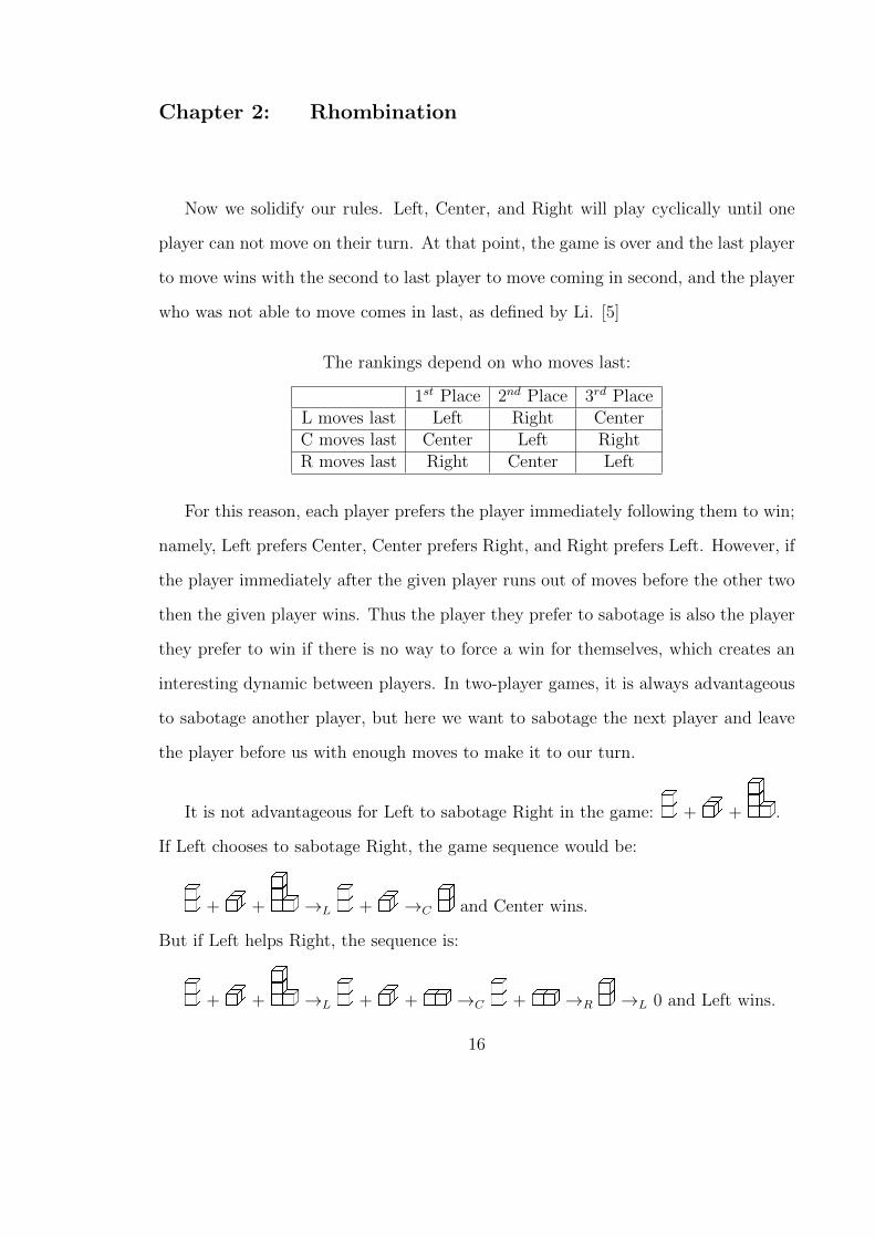
The rankings depend on who moves last:
1st Place 2nd Place 3rd PlaceL moves last Left Right CenterC moves last Center Left RightR moves last Right Center Left
For this reason, each player prefers the player immediately following them to win;
namely, Left prefers Center, Center prefers Right, and Right prefers Left. However, if
the player immediately after the given player runs out of moves before the other two
then the given player wins. Thus the player they prefer to sabotage is also the player
they prefer to win if there is no way to force a win for themselves, which creates an
interesting dynamic between players. In two-player games, it is always advantageous
to sabotage another player, but here we want to sabotage the next player and leave
the player before us with enough moves to make it to our turn.
It is not advantageous for Left to sabotage Right in the game: + + .
If Left chooses to sabotage Right, the game sequence would be:
+ + →L + →C and Center wins.
But if Left helps Right, the sequence is:
+ + →L + + →C + →R →L 0 and Left wins.
16
We now introduce the game on which we focus this research.
Rhombination is a three-player partizan game with perfect information and no
chance. The winner is determined by who moves last, which happens in a finite
number of turns.
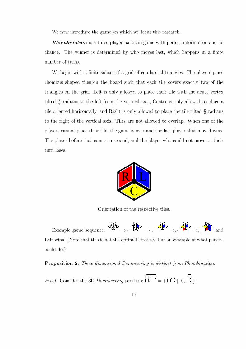
We begin with a finite subset of a grid of equilateral triangles. The players place
rhombus shaped tiles on the board such that each tile covers exactly two of the
triangles on the grid. Left is only allowed to place their tile with the acute vertex
tilted π6
radians to the left from the vertical axis, Center is only allowed to place a
tile oriented horizontally, and Right is only allowed to place the tile tilted π6
radians
to the right of the vertical axis. Tiles are not allowed to overlap. When one of the
players cannot place their tile, the game is over and the last player that moved wins.
The player before that comes in second, and the player who could not move on their
turn loses.
Orientation of the respective tiles.
Example game sequence: →L →C →R →L and
Left wins. (Note that this is not the optimal strategy, but an example of what players
could do.)
Proposition 2. Three-dimensional Domineering is distinct from Rhombination.
Proof. Consider the 3D Domineering position: = { || 0, }.
17
We want to show that this position can not be isomorphic to any Rhombination
position, where a three-player isomorphism is similarly defined as having the same
game trees, or isomorphic options, so we are looking for G = { || 0, }.
Since Right can take the whole board with one move, we can only have one
nontrivial component. Isolated triangles can be ignored in Rhombination because
they add nothing to the game, which we call trivial. Trivial components are and
. Also, triangles are not considered connected through corners, but through sides.
For instance, is two components, namely and .
Since Right can take the board in one move, the isomorphic Rhombination position
would be a Right tile with single triangles on the edges, which is a subset of .
Notice that we cannot have two nontrivial components or Right would not have a 0
option, so the game must be a single connected component with only trivial pieces
connected to the Right tile that can end the game.
As there are no center options, the side triangles cannot be included and the
subsets we are left with are: = {||0}, ∼= = {0||0}, and = { | | 0 }.
Thus there are no Rhombination games isomorphic to .
Therefore 3D Domineering and Rhombination are distinct.
We will now prove the fundamental theorem in a context of three players. Notice
that we name the players so we do not have to prove this is true in the three cases
with Left, Center, and Right moving first. Alex can be Left, Center, or Right, so
Beth and Charlie will be the naturally following players.
Theorem 2.1. (Fundamental Theorem of Combinatorial Games for Three Players)
Fix a game G played between Alex, Beth, and Charlie, with Alex moving first and
Beth moving second. When everyone plays in their best interest, exactly one of these
players can force a win with Alex moving first.
18
Proof. We will proceed by induction on the birthday of G.
Base Case: If G = 0, then when Alex plays first, he does not have a move on G, so
Charlie wins.
Assume the theorem is true for games born before day k. For G with birthday k,
note that all of Alex’s options allow someone to force a win with Beth moving first.
If Alex has an option where he can force a win when Beth moves first on that option,
he will pick that. If he has no options where he wins, but an option where Beth wins
moving first, he will take that so he gets second place. And if all his options allow
Charlie to force a win, then Charlie wins.
We make a strong assumption giving each player perfect strategy, but through
this we can always determine the winner of a game.
Now that we know the winner can always be determined, we can sort games into
outcome classes. We will notate these outcome classes by αβγ where α is the player
that wins when Left moves first, β is the player who wins when Center moves first,
and γ is the player who wins when Right moves first. This produces Table I. See
Appendix A for examples in Rhombination.
Some outcome classes to take special notice of are: LLL, CCC, RRR, LCR, CRL,
and RLC. LLL will be called L since it is a Left win. Similarly, CCC := C and RRR
:= R. LCR is a N ext player win, so LCR := N . RLC is a Previous player win, so
RLC := P . And lastly, CRL is a second player win, or an Other player win, so CRL
:= O.
Examples:
∈ L. ∈ C. ∈ R. ∈ N . + ∈ O. + + ∈ P .
By making observations on how options affect outcome classes, we generate Table
II, a three-player version of Table II from Chapter 1.
19

L wins when C goes firstL first
L wins C wins R wins
R firstL wins LLL CLL RLLC wins LLC CLC RLCR wins LLR CLR RLR
C wins when C goes firstL first
L wins C wins R wins
R firstL wins LCL CCL RCLC wins LCC CCC RCCR wins LCR CCR RCR
R wins when C goes firstL first
L wins C wins R wins
R firstL wins LRL CRL RRLC wins LRC CRC RRCR wins LRR CRR RRR
Table I: Three-Player Outcome Classes
some GC ∈ C some GR ∈ R some GR ∈ L ,all GR ∈ C
no GR ∈ Rsome GL ∈ L LCR LCL LCC
some GL ∈ C , no GL ∈ L CCR CCL CCCall GL ∈ R RCR RCL RCC
some GC ∈ R, no GC ∈ C some GR ∈ R some GR ∈ L ,all GR ∈ C
no GR ∈ Rsome GL ∈ L LRR LRL LRC
some GL ∈ C , no GL ∈ L CRR CRL CRCall GL ∈ R RRR RRL RRC
all GC ∈ L some GR ∈ R some GR ∈ L ,all GR ∈ C
no GR ∈ Rsome GL ∈ L LLR LLL LLC
some GL ∈ C , no GL ∈ L CLR CLL CLCall GL ∈ R RLR RLL RLC
Table II: Three-Player Effects of Options on Outcome
20
For example, let G ∈ LLL. Since Left wins moving first, there must be a position
Left can move on where Center moving next will allow Left to win, so there is a Left
option in L . Similarly, when Center moves first, there must be no option where
Center or Right wins, because Center prefers Left least, thus all the Center options
are in L. Right must have an option where Left wins, but could also have options
where Center wins, because they will choose Left to win, so there must be something
in L and there can be other options in C .
We will list the games of birthday 1 in Rhombination: There are seven possible
three-player games with birthday 1, namely:
{0||} = , {|0|} = , {||0} = ,
{|0|0} = , {0||0} = , {0|0|} = ,
{0|0|0} = .
For convenience, we will label four of these:
1L := {0||} = ∈ LLC, 1C := {|0|} = ∈ RCC,
1R := {||0} = ∈ RLR, ? := {0|0|0} = ∈ LCR.
It will be useful later to notate the sums of tiles such that for some number n,
nL = 1L + 1L + · · · + 1L (n times). We similarly define sums of other tiles, so for
example, 3C = 1C + 1C + 1C .
Proposition 3. We can set a recursive bound on the number of games with birthdays
of any size. If Gn is the set of all Rhombination games born by day n and gn = |Gn|,
then gn ≤ 23gn−1 and g0 = 1.
21
Proof. Since 0 is the only game with birthday 0, g0 = 1. Now for any G ∈ Gn, the
sets of options GL, GC , GR are contained in Gn−1. Since the number of subsets of an
m element set is 2m, we have gn ≤ 2gn−12gn−12gn−1 = 23gn−1 .
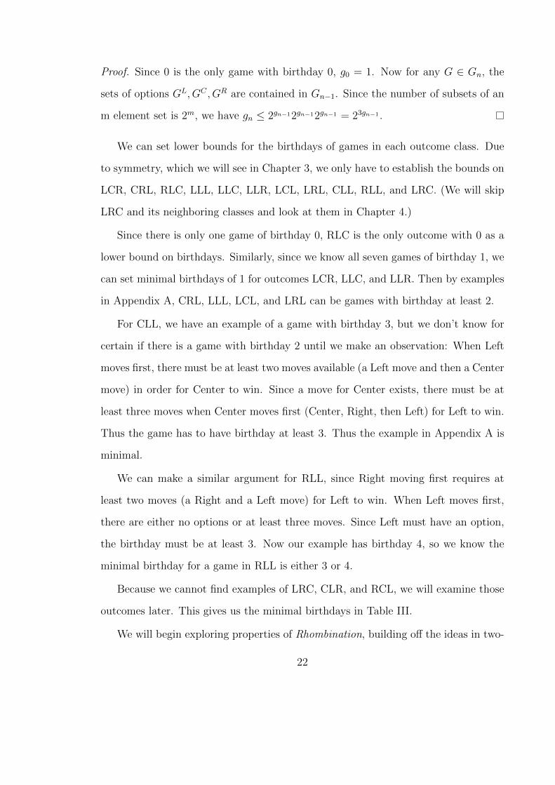
We can set lower bounds for the birthdays of games in each outcome class. Due
to symmetry, which we will see in Chapter 3, we only have to establish the bounds on
LCR, CRL, RLC, LLL, LLC, LLR, LCL, LRL, CLL, RLL, and LRC. (We will skip
LRC and its neighboring classes and look at them in Chapter 4.)
Since there is only one game of birthday 0, RLC is the only outcome with 0 as a
lower bound on birthdays. Similarly, since we know all seven games of birthday 1, we
can set minimal birthdays of 1 for outcomes LCR, LLC, and LLR. Then by examples
in Appendix A, CRL, LLL, LCL, and LRL can be games with birthday at least 2.
For CLL, we have an example of a game with birthday 3, but we don’t know for
certain if there is a game with birthday 2 until we make an observation: When Left
moves first, there must be at least two moves available (a Left move and then a Center
move) in order for Center to win. Since a move for Center exists, there must be at
least three moves when Center moves first (Center, Right, then Left) for Left to win.
Thus the game has to have birthday at least 3. Thus the example in Appendix A is
minimal.
We can make a similar argument for RLL, since Right moving first requires at
least two moves (a Right and a Left move) for Left to win. When Left moves first,
there are either no options or at least three moves. Since Left must have an option,
the birthday must be at least 3. Now our example has birthday 4, so we know the
minimal birthday for a game in RLL is either 3 or 4.
Because we cannot find examples of LRC, CLR, and RCL, we will examine those
outcomes later. This gives us the minimal birthdays in Table III.
We will begin exploring properties of Rhombination, building off the ideas in two-
22
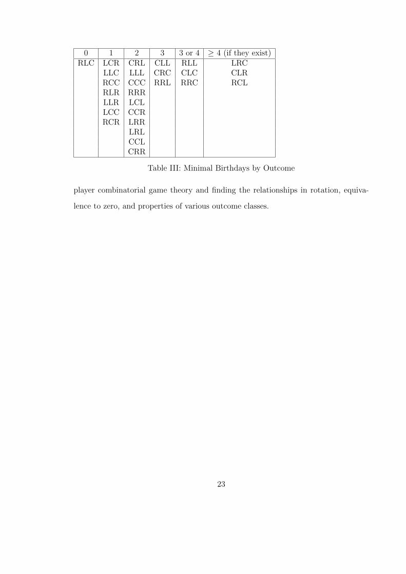
0 1 2 3 3 or 4 ≥ 4 (if they exist)RLC LCR CRL CLL RLL LRC
LLC LLL CRC CLC CLRRCC CCC RRL RRC RCLRLR RRRLLR LCLLCC CCRRCR LRR
LRLCCLCRR
Table III: Minimal Birthdays by Outcome
player combinatorial game theory and finding the relationships in rotation, equiva-
lence to zero, and properties of various outcome classes.
23
Chapter 3: Comparisons, Posets, and Symmetry
In two-player games, all games in the outcome class P are equal to the zero game.
It would be nice to find a similar result in the three-player Previous outcome class,
RLC. However, by Cincotti’s definitions, this is not true.
3.1 Cincotti’s Approach to Partial Order
Consider the game 1L + 1C + 1R ∈ RLC. We would expect this game to equal 0 since
any sum gives each player one extra move and should not affect the outcome of a
game.
In [6], Cincotti defines≥ with respect to each of the players with the antisymmetric
property. For example, G =L H iff (G ≥L H and G ≤L H). General equality holds if
games are equal with respect to all three players, meaningG = H iffG =L H,G =C H,
and G =R H. Following Cincotti, we have the following definition.
Definition 8. For games G and H, G ≥L H iff [(H ≥L no GC) and (H ≥L no GR)
and (no HL ≥L G)].
Using this and the fact that 0 = {||}, we simplify the definition to compare to 0:
Definition 9. For game G, G ≥L 0 iff (0 ≥L no GC and 0 ≥L no GR). 0 ≥L G iff
(no GL ≥L 0).
We will compute the Left comparison to 0 for games 1L, 1C , and 1R. 1L has no
Center or Right options, but the Left option is 0, so 1L>L0. 1C has a 0 Center option,
so 1C 6≥L 0. 1C no Left options, so 0 ≥L 1C . Thus 0>L1C . Similarly, 0>L1R.
Proposition 4. By Cincotti’s definition, 1L + 1C + 1R ∈ RLC = P is not equal to 0.
24

Proof. LetG = 1L+1C+1R = {1C+1R|1L+1R|1L+1C} = {∅|1R|1C ||1R|∅|1L||1C |1L|∅}.
Now 0 ≥L G ⇔ no GL ≥L 0 ⇔ {|1R|1C} �L 0 ⇔ (0 ≥L 1R or 0 ≥L 1C) which is
true. Thus 0 ≥L G.
Now G ≥L 0 ⇔ (0 ≥L no GC and 0 ≥L no GR) ⇔ (0 �L {1R||1L} and 0 �L
{1C |1L|}) ⇔ (1R ≥L 0 and 1C ≥L 0) which is false, so G �L 0.
Therefore 0>LG, so G 6= 0.
This is less than ideal, so we will use the definitions of equality and ≥ with respect
to different players in a generalization of the two-player definition.
3.2 Our Approach
We establish an equivalence for games. This parallels the two-player equivalence,
looking at outcomes, instead of comparing options recursively as Cincotti defines.
Definition 10. For games G and H, G = H means for all games X, G+X has the
same outcome as H +X.
Proposition 5. = is an equivalence relation.
Proof. Fix a game X.
Reflexive: G+X has the same outcome class at G+X, so G = G.
Symmetric: If G = H, then G + X and H + X have the same outcome, thus
H = G.
Transitive: Let G = H and H = K. G + X has the same outcome as H + X,
which has the same outcome as K +X, so G+X has the same outcome as K +X.
Thus G = K.
Lemma 2. For a game G, G+ 0 = G.
25

Proof. We will induct on the birthday of G.
Base Case: G = 0. Then 0+0 = {||}+{||} = {∅+0, 0+∅|∅+0, 0+∅|∅+0, 0+∅} =
{∅, ∅|∅, ∅|∅, ∅} = {||} = 0.
Assume G+ 0 = G for G born before day k. Now for G with birthday k:
G+ 0 = {GL|GC |GR}+ {||}
= {GL + 0, G+ ∅|GC + 0, G+ ∅|GR + 0, G+ ∅}
= {GL + 0|GC + 0|GR + 0} = {GL|GC |GR} = G.
Thus, by induction, G+ 0 = G.
Theorem 3.1. For a game G, G = 0⇒ G ∈ P.
Proof. Let G = 0. This means ∀X, G+X and 0+X have the same outcome. Choose
X = 0. Now G+ 0 = G and 0 + 0 = 0 ∈ P have the same outcome, so G ∈ P .
We conjecture that the converse is true in Chapter 4. Next we solidify our defini-
tion of game inequality, which we will use from here on.
Definition 11. For games G and H, G ≥L H means for all games X, Left wins G+X
whenever Left wins H +X. (Meaning Left wins H +X ⇒ Left wins G+X.)
Proof of well-definedness: Let G and H be games such that G ≥L H. Suppose G’ and
H’ are games such that G = G′ and H = H ′. Then ∀X, Left wins H ′+X means Left
wins H + X, which implies Left wins G + X, which means Left wins G′ + X. Thus
G′ ≥L H ′.
The relation ≥L is also reflexive, transitive, and antisymmetric, which gives us a
partially ordered set.
Proposition 6. The combination of all partial orders: G ≥L H, H ≥L G, G ≥C H,
H ≥C G, G ≥R H, and H ≥R G implies that G = H.
26

≥L 0 1L 1C 1R ≥C 0 1C 1R 1L ≥R 0 1R 1L 1C0 � × � × 0 � × � × 0 � × � ×1L � � � × 1C � � � × 1R � � � ×1C × × � × 1R × × � × 1L × × � ×1R � × � � 1L � × � � 1C � × � �
Left Poset: ≥L Center Poset: ≥C Right Poset: ≥R
1L1R
1C1L
1R1C
0
1C
0
1R
0
1L
BBBB
���
BBBB
���
BBBB
���
Figure 3.1: The Posets of 1L, 1C , 1R, and 0
Proof. Fix a game X. Now we look at the outcomes of G+X and H+X. By G ≥L H,
we know Left wins on G + X whenever Left wins on H + X. Also by H ≥L G, we
know Left wins on H +X whenever Left wins on G+X. So Left must win on G+X
if and only if Left wins on H + X. By a similar argument, Center and Right must
win on G+X under the exact same conditions as H +X. Thus G+X and H +X
must have the same outcomes.
By these definitions, we develop Figure 3.1.
Proofs and examples for Figure 3.1:
• 1L ≥L 0: If Left wins X, then Left wins X + 1L, because Center will still run
out of moves first.
• 1C �L 0: Left wins going third on 0, but not on 1C .
• 1R ≥L 0: If Left wins X, Center runs out of moves first, so in X + 1R, Center
will still run out of moves before Right or Left.
27

• 0 �L 1L: Left wins going first on 1L, but not on 0.
• 1C �L 1L: Left wins going first on 1L, but not on 1C .
• 1R �L 1L: Left wins going first on 1L, but not on 1R.
• 0 ≥L 1C : If Left wins X + 1C , then Center runs out of moves first in X + 1C ,
so Center will still run out of moves first in X.
• 1L ≥L 1C : Transitively, since 1L ≥L 0 and 0 ≥L 1C .
• 1R ≥L 1C : Transitively, since 1R ≥L 0 and 0 ≥L 1C .
• 0 �L 1R: Left wins going second on 1L + 1R, but not on 1L.
• 1L �L 1R: Left wins going second on 1L + 1R, but not on 1L + 1L.
• 1C �L 1R: Left wins moving third on 1R, but not on 1C .
Proposition 7. For any player α, and for games G, H, and K, if G ≥α H, then
G+K ≥α H +K.
Proof. Let X be any game. If α wins (H+K)+X = H+(K+X), then since K+X is
a game, α must also win G+(K+X) = (G+K)+X. Therefore G+K ≥α H+K.
3.3 Rotations and Reflections
Definition 12. For a game G, we define G60 as the counter-clockwise rotation
of G by π3
radians.
Examples:60
= ,60
= , and60
= .
28
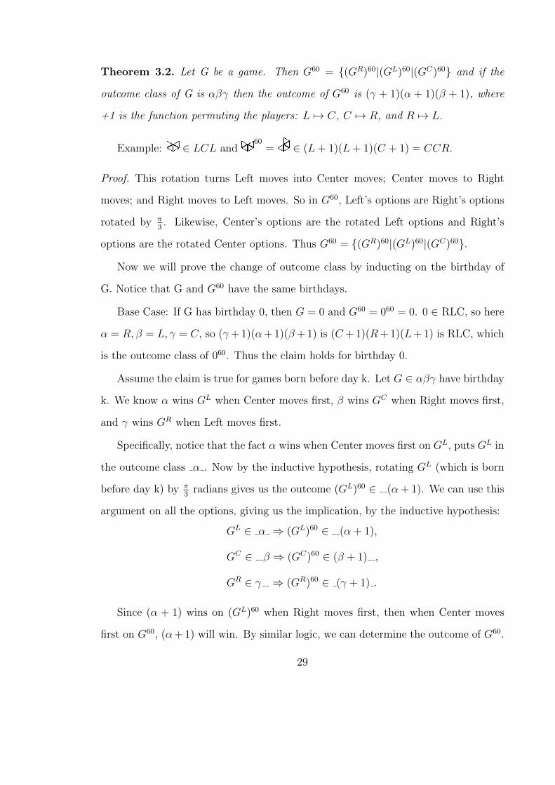
Theorem 3.2. Let G be a game. Then G60 = {(GR)60|(GL)60|(GC)60} and if the
outcome class of G is αβγ then the outcome of G60 is (γ + 1)(α + 1)(β + 1), where
+1 is the function permuting the players: L 7→ C, C 7→ R, and R 7→ L.
Example: ∈ LCL and60
= ∈ (L+ 1)(L+ 1)(C + 1) = CCR.
Proof. This rotation turns Left moves into Center moves; Center moves to Right
moves; and Right moves to Left moves. So in G60, Left’s options are Right’s options
rotated by π3. Likewise, Center’s options are the rotated Left options and Right’s
options are the rotated Center options. Thus G60 = {(GR)60|(GL)60|(GC)60}.
Now we will prove the change of outcome class by inducting on the birthday of
G. Notice that G and G60 have the same birthdays.
Base Case: If G has birthday 0, then G = 0 and G60 = 060 = 0. 0 ∈ RLC, so here
α = R, β = L, γ = C, so (γ+ 1)(α+ 1)(β+ 1) is (C + 1)(R+ 1)(L+ 1) is RLC, which
is the outcome class of 060. Thus the claim holds for birthday 0.
Assume the claim is true for games born before day k. Let G ∈ αβγ have birthday
k. We know α wins GL when Center moves first, β wins GC when Right moves first,
and γ wins GR when Left moves first.
Specifically, notice that the fact α wins when Center moves first on GL, puts GL in
the outcome class α . Now by the inductive hypothesis, rotating GL (which is born
before day k) by π3
radians gives us the outcome (GL)60 ∈ (α+ 1). We can use this
argument on all the options, giving us the implication, by the inductive hypothesis:
GL ∈ α ⇒ (GL)60 ∈ (α + 1),
GC ∈ β ⇒ (GC)60 ∈ (β + 1) ,
GR ∈ γ ⇒ (GR)60 ∈ (γ + 1) .
Since (α + 1) wins on (GL)60 when Right moves first, then when Center moves
first on G60, (α+ 1) will win. By similar logic, we can determine the outcome of G60.
29
Therefore G60 = {(GR)60|(GL)60|(GC)60} ∈ (γ + 1)(α + 1)(β + 1).
A game G is rotationally symmetric when G60 is the exact same as G. For
example,60
is the same as .
Corollary 1. If G ∈ αβγ is rotationally symmetric, then G ∈ LCR,RLC, or CRL.
Proof. Let G ∈ αβγ be rotationally symmetric. Then G60 will be in the same outcome
class as G, so α = (γ + 1), β = (α + 1), γ = (β + 1).
Case 1: α = L. Then β = L+ 1 = C and γ = C + 1 = R, so G ∈ LCR.
Case 2: α = C. Then β = C + 1 = R and γ = R + 1 = L, so G ∈ CRL.
Case 3: α = R. Then β = R + 1 = L and γ = L+ 1 = C, so G ∈ RLC.
Notice that the converse is not true. For example, ∈ CRL, but is clearly not
rotationally symmetric.
Corollary 2. G180 is isomorphic to G.
Proof. First notice:
G = {GL|GC |GR},
G60 = {(GR)60|(GL)60|(GC)60},
(G60)60 = G120 = {(GC)120|(GR)120|(GL)120},
((G60)60)60 = G180 = {(GL)180|(GC)180|(GR)180}.
We will induct on the birthday of G. Base Case: 0 ∼= 0180.
Assume this is true for games born before day k. Now let G have birthday k.
So G = {GL|GC |GR} ∼= {(GL)180|(GC)180|(GR)180} = G180.
Definition 13. The dihedral motions of a hexagon are the cyclic permutation
representations of the rigid motions of a regular hexagon, with corners labeled below.
30
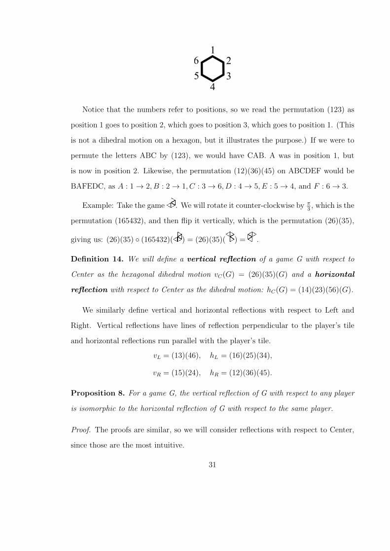
Notice that the numbers refer to positions, so we read the permutation (123) as
position 1 goes to position 2, which goes to position 3, which goes to position 1. (This
is not a dihedral motion on a hexagon, but it illustrates the purpose.) If we were to
permute the letters ABC by (123), we would have CAB. A was in position 1, but
is now in position 2. Likewise, the permutation (12)(36)(45) on ABCDEF would be
BAFEDC, as A : 1→ 2, B : 2→ 1, C : 3→ 6, D : 4→ 5, E : 5→ 4, and F : 6→ 3.
Example: Take the game . We will rotate it counter-clockwise by π3, which is the
permutation (165432), and then flip it vertically, which is the permutation (26)(35),
giving us: (26)(35) ◦ (165432)( ) = (26)(35)( ) = .
Definition 14. We will define a vertical reflection of a game G with respect to
Center as the hexagonal dihedral motion vC(G) = (26)(35)(G) and a horizontal
reflection with respect to Center as the dihedral motion: hC(G) = (14)(23)(56)(G).
We similarly define vertical and horizontal reflections with respect to Left and
Right. Vertical reflections have lines of reflection perpendicular to the player’s tile
and horizontal reflections run parallel with the player’s tile.
vL = (13)(46), hL = (16)(25)(34),
vR = (15)(24), hR = (12)(36)(45).
Proposition 8. For a game G, the vertical reflection of G with respect to any player
is isomorphic to the horizontal reflection of G with respect to the same player.
Proof. The proofs are similar, so we will consider reflections with respect to Center,
since those are the most intuitive.
31

Geometrically consider what reflections do to the options of G. Both reflections
preserve Center’s moves and switch the moves of Left and Right, giving us:
vC(G) = {vC(GR)|vC(GC)|vC(GL)} and hC(G) = {hC(GR)|hC(GC)|hC(GL)}.
Now we will induct on the birthday of G:
Base Case: G = 0. Then vC(0) = 0 = hC(0).
Assume the theorem is true for games born before day k, and now for G with
birthday k:
vC(G) = {vC(GR)|vC(GC)|vC(GL)} ∼= {hC(GR)|hC(GC)|hC(GL)} = hC(G).
Consider the games , , and . We will look at the vertical and horizontal
reflections with respect to each player.
With respect to Left:
vL( ) = , hL( ) = ,
vL( ) = , hL( ) = ,
vL( ) = , hL( ) = .
With respect to Center:
vC( ) = , hC( ) = ,
vC( ) = , hC( ) = ,
vC( ) = , hC( ) = .
With respect to Right:
vR( ) = , hR( ) = ,
vR( ) = , hR( ) = ,
vR( ) = , hR( ) = .
32

Chapter 4: Future Directions
4.1 Additional Concepts to Prove
Continuing to build on two-player game theory, we have a few unproven conjectures.
We would naturally like to find the set of games that do not change the outcome of
other games, leading to the first conjecture:
Conjecture 1 (Converse of Theorem 3.1). If G ∈ P then G = 0.
Currently the set of Rhombination game positions under addition is an abelian
monoid since we have a closed, associative, and commutative operation with an iden-
tity. However our identity is very limited, being only the game 0. If we can prove
Conjecture 1, we would have a more generalized identity we can use more easily in
proofs which could also help us find inverses.
We do not have a proof for Conjecture 1; however, we have looked into showing
the particular game 1L + 1C + 1R ∈ P is equal to 0 through induction, though we
have only figured out some of the cases.
In order to show 1L + 1C + 1R = 0, we need to show for any game H, that
H + 1L + 1C + 1R has the same outcome as H. We will attempt strong induction on
the birthday of H:
Base Case: H = 0. Then by Lemma 2, H + 1L + 1C + 1R = 1L + 1C + 1R ∈ P and
H ∈ P , so it holds.
Now we assume H + 1L + 1C + 1R has the same outcome as H for any H born
before day k. For each player moving first, the argument is similar, so suppose Left
is moving first on this position.
Case 1: Left moves on H. Then we have HL + 1L + 1C + 1R which has the same
33
outcome as HL. By the inductive hypothesis, 1L + 1C + 1R does not change the
outcome.
Case 2: Left moves on 1L. Then we are left with H + 1C + 1R. This is where
it gets complicated. If Center and Right both move on 1C and 1R respectively, then
after one cycle we have Left moving first on H and nothing is changed.
However, if Center and Right do not follow and we end up with a position like
HC +1C , then we do not know what happens to the outcome since we only know who
wins HC when Right moves first. Thus our conjecture remains unproven, even for a
simple position like 1L + 1C + 1R.
Conjecture 2. There are no Rhombination games in LRC, CLR, or RCL.
So far, we have not found or been able to create a game that falls in any of these
outcome classes, so we wonder if they may be empty.
Proposition 9. A Rhombination game in LRC, if it exists, must have birthday at
least 4.
Proof. The fact that Left wins moving first implies we have to have birthday at least
1. Right wins when Center moves first means we need birthday at least 2 since Center
and Right need successive moves. Center wins when Right moves first means that
Right has either no options or there are at least 3 moves. Right has to have an option
since they win when Center moves first, so there is a Right move. Thus, there has to
be a Right move followed by a Left and Center move, making the game have birthday
at least 3.
Left cannot win in one move because that would be isomorphic to a subset of
(see Proposition 2 for reasoning), which has birthday no greater than 2, so it cannot
be in LRC. Thus Left’s option must have a Left, Center, Right, and Left move for
Left to win, giving us a birthday of at least 4.
34

Since games in LRC, CLR, and RCL are equivalent up to rotation, the same result
applies to CLR and RCL.
Conjecture 3. Assuming Conjecture 1, for a game G, G + G60 + G120 ∈ P, which
gives us the inverse: −G = G60 + (G60)60.
If the proposed identity from Conjecture 1 and inverses from Conjecture 3 can be
proven to work properly, that would make the set of Rhombination games an abelian
group under game addition.
It would be convenient to have some form of trimming moves like we have in
creating canonical form for two-player games. We want to show we can remove
dominated options, which means for A,B ∈ GL, if B ≥L A, then GL = GL −A. The
interesting problem we run into with three players is we do not necessarily know that
a player will always pick the option that dominates with respect to themselves. If a
winning strategy does not exist, they will aim to help the player after them.
For example, if Left had options like 1C and 1C +1R, then even though 1C +1R ≥L
1C , Left is going to choose 1C because then Left will come in second place instead of
third. (Now this set of options may not be possible, but the concept is still something
we have to consider.)
Reversible options are even more tricky to determine. The idea behind them in
two-player games is that if one player can respond to the move of another with a game
that is more favorable than the original, then we can bypass that option. However,
since a player has to respond to the moves of two other players, this is difficult to
imagine an analog to.
In this paper, we assume perfect strategy from all three players, but we think it
is sufficient to only have the first and second place winners play optimally.
35
4.2 Number Games
It would be useful to quantify the benefit of a position for a certain player. This
property in two-player games are called number games. When a two-player game is
a number, we can immediately determine the outcome class along with total ordering
with respect to any player compared to any other number games. Since the number
line is not three-directional, it is difficult to extend this system to three players.
In two-player games, our numbers are one-dimensional, where positive numbers
help Left and negatives help Right. We cannot add a third player to this system,
so we will expand the two-player number games to the plane in R2, where Left’s
advantage is in the x-direction and Right’s is in the y-direction. Notice that when
we consider sums of number games such as and , we create a line of equivalence
classes which form a bijection with the x-axis: R. For instance, 3( )+2( ) = (3,2)
in these coordinates, which belongs to the equivalence class with x-intercept 1, so
(3,2) = (2,1) = (1,0).
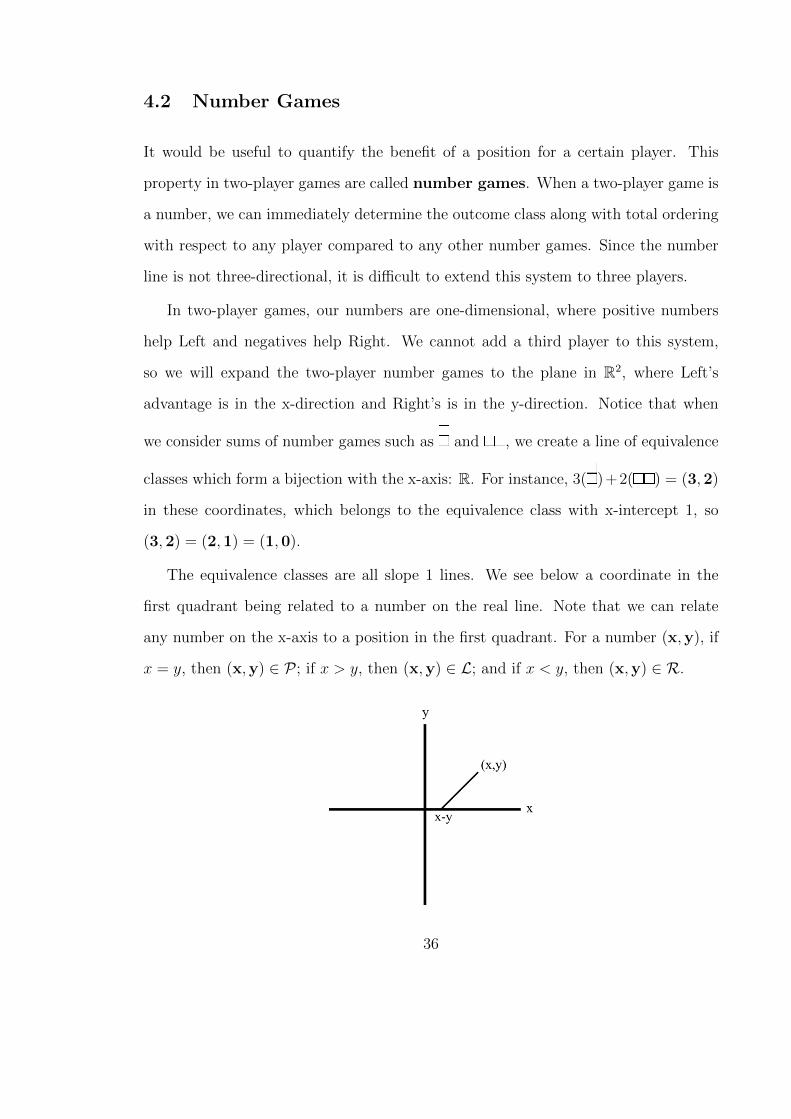
The equivalence classes are all slope 1 lines. We see below a coordinate in the
first quadrant being related to a number on the real line. Note that we can relate
any number on the x-axis to a position in the first quadrant. For a number (x,y), if
x = y, then (x,y) ∈ P ; if x > y, then (x,y) ∈ L; and if x < y, then (x,y) ∈ R.
36

This provides the intuition for our approach to three-player number games.
In defining this, perhaps if we could quantify the amount a game benefits a specific
player, we could find three-dimensional coordinates in the first quadrant for a game.
We will build these number games exclusively on sums of tiles, i.e. a( )+b( )+c( ).
We define an (x, y, z)-coordinate value by first assigning the value (1,0,0) to the
smallest LLL game, + . Similarly, we will assign (0,1,0) to + and (0,0,1)
to + .
Example: A number (1,2,3) would be: 1( + ) + 2( + ) + 3( + ) =
3( ) + 5( ) + 4( ) = 3L + 5C + 4R ∈ RRR.
A quick look at some basic sums gives us:
(0,0,0) ∈ RLC (1,1,1) ∈ RLC
(1,0,0) + (1,0,0) = (2,0,0) ∈ LLL (1,0,0) + (0,1,0) = (1,1,0) ∈ LLC
(0,1,0) + (0,1,0) = (0,2,0) ∈ CCC (0,1,0) + (0,0,1) =(0,1,1) ∈ RCC
(0,0,1) + (0,0,1) = (0,0,2) ∈ RRR (1,0,0) + (0,0,1) =(1,0,1) ∈ RLR
The outcome of these games depends solely on who runs out of tiles first, as
(x,y, z) = (x+ y) + (y+ z) + (x+ z) . Once a player runs out of tiles, the player
before them wins.
Conjecture 4. Number games form an equivalence class where (x,y, z) = (u,v,w)
if and only if x− u = y − v = z − w.
This seems intuitive enough, but since we have not been able to prove that 1L +
1C + 1R = 0, we cannot show this in general yet.
How many outcomes can we produce with numbers and what can we generalize
about them? We observe the following properties:
1. If x = y = z = 0, then (x,y, z) ∈ RLC.
This is given by (x,y, z) = (0) + (0) + (0) = 0 ∈ RLC.
37

2. If x > y ≥ 0, z = 0, then (x,y, z) ∈ LLL.
This is given by (x,y, z) = (x+ y) + (y) + (x) , so Center will run out of moves
first and Left will always win.
3. If x = y > 0, z = 0, then (x,y, z) ∈ LLC.
This is given by (x,y, z) = (2x) + (x) + (x) , which means Center will run out of
moves first unless Right moves first.
4. If y > x > 0, z = 0, then (x,y, z) ∈ CCC.
This is given by (x,y, z) = (x + y) + (y) + (x) , so Right will run out of moves
first and Center will always win.
Properties 1-4 are sufficient to classify the outcomes of all number games for two
reasons:
Firstly, if a = min{x, y, z}, then (x,y, z) belongs to the same outcome class as
(x− a,y − a, z− a). This is because subtracting a from all three coordinates is the
same as removing 2a rounds of turns, which do not affect the outcome of the game.
Thus the cases where one of x, y, z equal 0 are enough to determine the outcome.
Secondly, rotations permute our numbers, so since (1,0,0)60 = (0,1,0), we can
similarly argue that (x,y, z)60 = (z,x,y). Thus the outcomes in all other cases can
be found by rotation.
We are saying that given any number game (x,y, z), we can reduce at least one
of the coordinates to zero without changing the outcome and then rotate to make
z = 0, which has a well-defined effect on the outcome, and then the resulting game
will follow one of the four given properties.
Thus by reduction and rotation, we can only produce the outcomes RLC, LLL,
CCC, RRR, LLC, RCC, and RLR through these number games.
Now that we have number games and understand them fairly well, the questions
are how do we generalize them and what do they mean? We can see definite benefits
38

to each player given different sums, so it would be interesting to better understand
how we might generalize numbers in order to apply them to more complicated game
positions.
This thesis provides the foundation for this research by solidifying game rules and
definitions in Rhombination and other three-player partizan games. We have made
some discoveries such as the effect of rotation on outcome and created an abelian
monoid with an identity we wish to generalize. The most important next step would
be to prove a generalized identity for game addition along with finding inverses to
games to give us an abelian group. Another important idea to look for is the existence
or nonexistence of positions in the outcome classes LRC, CLR, and RCL.
39
Bibliography
[1] Albert, Nowakowski, and Wolfe. Lessons in Play, A K Peters Ltd., Wellesley,
Massachusetts, 2007.
[2] Skiena, S. Hasse Diagrams. Computational Discrete Mathematics, Cambridge
University, 5.4.2, 2003.
[3] Cincotti, Alessandro. Three-player Domineering. International Journal of Math-
ematical, Computational, Physical, Electrical and Computer Engineering, Vol. 2,
No. 10, 2008.
[4] Propp, James. Three-player impartial games. Department of Mathematics, Uni-
versity of Wisconsin, 1998.
[5] Li, S.-Y.R. N-person Nim and N-person Moore’s Games. International Journal
of Game Theory, Vol. 7, Issue 1, page 31-36, 1978.
[6] Cincotti, A. Three-player partizan games. Theoretical Computer Science 332
(2005) 367-389. Engineering Vol: 2, No: 10, 2008.
40

Appendix A: Rhombination Positions for the Outcome
Classes
∈ LCR + ∈ CRL ∈ RLC
+ ∈ LLL + ∈ CCC + ∈ RRR
∈ LLC ∈ RCC ∈ RLR
∈ LLR ∈ LCC ∈ RCR
∈ LCL ∈ CCR ∈ LRR
+ ∈ LRL + ∈ CCL + ∈ CRR
∈ CLL ∈ CRC ∈ RRL
∈ RLL ∈ CLC ∈ RRC
? ∈ LRC ? ∈ CLR ? ∈ RCL
These game examples have minimal birthdays except for RLC, RLL, CLC, and
RRC. We do not have minimal examples for RLL, CLC, and RRC, but the minimal
RLC game is 0.
41

Appendix B: Sample Game Trees for Rhombination
We will highlight the optimal game sequences in green.
����
����
���
����
����
���
����
����
���
�����
���
CCCC
CCCC
CCCC
@@
@@
@@
@@
@@@
@L L C R
����
AAAA
����
AAAA
����
����
����
����
L R L C L L
This game is in LCL.
����
����
���
����
����
���
����
����
���
���
���
��
HHHHH
HHH
HHH
HHHHH
HHHH
HHHH
PPPP
PPPP
PPP
PPPP
PPPP
PPP
PPPP
PPPP
PPP
L L C C R
����
����
@@@
@
����
AAAA
����
AAAA
����
����
����
AAAA
L L C R C R L C L C
This game is also in LCL.
42

+
���
���
��
HHH
HHH
HH
HHH
HHH
HH
HHHH
HHH
H
R R
+
����
@@@@
����
����
����
@@
@@L L L L
C C C
This is a partial game tree in RLL where we look at the sequence with Right
moving first.
43

Curriculum Vitae : Katie Greene
Education:
Wake Forest University
Master of Arts in Mathematics
May 2017
Brigham Young University
Bachelor of Science in Mathematics
December 2014
Professional Experience:
Site Director at AoPS Academy (March 2017-Present)
Graduate Teaching Assistant at Wake Forest (August 2015-May 2017)
Grader for Measurement Incorporated (February 2015-July 2015)
Discrete Math Grader for Brigham Young University (January 2013-April 2014)
Math Circles Assistant for Brigham Young University (September 2013- April 2014)
PALS Math Teacher for Timpanogos Elementary (December 2013 - April 2014)
MathCounts Coach for Lakeridge Junior High (December 2013 - March 2014)
Math Tutor for Forsyth Tech (February 2011 - December 2011)
Performance Experience
Independent Performer with the Tricky Trio (February 2015 - May 2016)
Actress/Choreographer for Showtime Performers (July 1998 - August 2015)
Acrobat for the Carolina Renaissance Festival (October 2006 - November 2009)
44