exploration of long run carbon-intensive pathways with ... · ‘routine’ behaviors. for...
TRANSCRIPT
20 rue Rosenwald 75015 PARIS
Teacutel 01 53 68 14 94 Fax 01 53 68 14 93
NEW EMISSIONS SCENARIOS
Exploration of long run carbon-intensive pathways with IMACLIM-R
ENSEMBLES Project Task 71b
February 2007
- 1 -
Partner
60 SMASH 20 rue Rosenwald 75015 PARIS France
Contact
Jean-Charles HOURCADE 45bis avenue de la Belle Gabrielle 94736 Nogent-Sur-Marne cedex (33) 1 43 94 73 80 hourcadecentre-ciredfr
Team
CRASSOUS Renaud GITZ Vincent GUIVARCH Ceacuteline SASSI Olivier WAISMAN Henri
- 2 -
1 INTRODUCTION 4
2 THE IMACLIM-R FRAMEWORK 6 21 RATIONALE OF THE IMACLIM-R MODELING BLUEPRINT 6
211 A Dual Vision of the Economy an easier dialogue between engineers and economists 7 212 A growth engine allowing gaps between potential and real growth 10
22 TECHNICAL DESCRIPTION 11 221 Aggregation scheme and Data 11 222 Static Equilibrium 14 223 Dynamic Linkages Growth engine and technical change 25
3 LONG-RUN EMISSION SCENARIOS 33 31 ASSUMPTIONS 33
311 The growth engine 33 312 Development styles laquo energy intensive raquo vs laquo energy sober raquo 36 313 Energy and technology variables variants on technical progress and on the speed of technology diffusion 37 314 Eight alternative scenarios 38
32 EMISSION SCENARIOS 39 321 What risks of a high carbon future 39 322 The laquo Kaya raquo decomposition revisited ex post 40 323 The rebound effects 43 324 The structural change in the developing countries 47 325 The comeback of coal 49 326 Impact of growth variants on the fossil content of trajectories 51
33 CONCLUSION 51
4 REFERENCES 53
- 3 -
1 Introduction
This report deals with the research undertaken for the ENSEMBLES European Project at SMASH-CIRED under the Research Theme 7 lsquoScenarios and policy Implicationsrsquo precisely to fulfill Task 71b
Task 71 was first focused on the assessment of SRES scenarios which provided the clear answer that SRES trajectories were still a valid set of reference scenarios to explore the range of uncertainties about non-intervention future pathways (Tol OrsquoNeill van Vuuren 2005 Vuuren and ONeill 2006) SMASH was involved in the updated task 71b that was to compute some new emissions scenarios that could bring further insights beyond the materials and lessons from SRES The SRES exercise was a unique attempt to provide a set of scenarios explicitly designed to explore the uncertainties both from models and from our ignorance of the future This kind of exercise demands a rigorous coordination scheme stringent transparency on modeling assumptions numerous iterations among experts and modelers and numerous model runs Therefore both for scientific and for pragmatic reasons the research presented in this report do not pretend to provide a new updated comprehensive set of trajectories but rather intend to focus on a specific question
One major challenge is to reinforce the internal consistency of long run
scenarios through an endogenous representation of the interactions between macroeconomic technological and structural variables The Imaclim-R model aims precisely at allowing a representation detailed enough as to reinforce the plausibility of the simulated trajectories and facilitating the dialog between modellers experts and stakeholders Two research issues are at stake in this innovative modelling approach
(i) On one side a stronger consistency could probably limit the uncertainty of emission trajectories if some combinations of exogenous trends are deemed to be impossible
(ii) On the other side the modelling of endogenous mechanisms instead of exogenous trends should in principle lead to more robust assessments of the impact from energy and climate policies owing to an explicit modelling of more numerous possible feedbacks
We chose to apply this approach to try and explore scenarios that could be in the
upper bound of carbon-intensive pathways This choice stems from two facts in the current research community
(i) In many studies we observed that the multi-scenario approach is somehow abandoned in favor of a single medium reference trajectory which we think very harmful for policy-oriented as academic research
- 4 -
(ii) Recent trends of energy and carbon intensity led to a strong increase of emissions that is follows the upper bound of the SRES scenarios in spite of the ETS the Kyoto Protocol and the plausibility of future stringent GHG regulations This means that some deep forces ndash growth technology or development styles ndash actually push emissions upwards and are likely to do so during the following decades more than sometimes expected on average
Understanding what are the forces behind a carbon-intensive scenario could play a
significant role in the design of appropriate policies in due time to counterbalance these forces and lead the economy on a decarbonization path
The report is divided in two parts first it presents the Imaclim-R model its
rationale and its detailed specifications second it presents a set of emission scenarios computed with Imaclim-R thanks to the most recent developments The new scenarios explore what could be the energy and non-energy drivers of high emissions trajectories We focus our analysis on the link between trajectory uncertainty and the interactions between global growth regimes price signals technology potentials and development styles
2 The Imaclim-R framework
The risk of non sustainable development stems ultimately from the joint effect of issues as diverse as climate change energy and food security land cover changes or social dualism in urban and rural areas These issues in turn depend on the dynamics of consumption and technologies in sectors such as energy transportation construction or food production and on the hazards caused by shortages of primary resources or by the transformation of our global environment The challenge is thus to integrate sector-based analysis in a common economic framework capturing their interplay in a world experiencing very rapid demographic and economic transitions
The IMACLIM-R structure presented in this paper tries and meets this challenge through an integrated modeling approach (Weyant et al 1996) Its primary aim is to provide an innovative framework that could organize better the dialogue between economics (to capture the general interdependences between sectors issues and policy decisions) demography (to represent a major driver of the world economic trends) natural sciences (to capture the feedbacks of the alteration of the ecosystems) and engineering sciences (to capture the technical constraints and margins of freedom)
We first present the rationale of the IMACLIM-R structure the following part contains the technical description of its static and dynamic components
21 Rationale of the IMACLIM-R modeling blueprint
The overall rationale of IMACLIM-R stems from the necessity to understand better amongst the drivers of baseline and policy scenarios the relative role of (i) technical parameters in the supply side and in the end-use equipments (ii) structural changes in the final demand for goods and services (dematerialization of growth patterns) (iii) micro and macroeconomic behavioral parameters in opened economies This is indeed critical to capture the mechanisms at play in transforming a given environmental alteration into an economic cost and in widening (or narrowing) margins of freedom for mitigation or adaptation
The specific way through which IMACLIM-R tries and reaches this objective
derives from a twofold diagnosis about the challenges for designing more useful baseline scenarios
minus The increasing recognition that endogenizing technical change to capture policy induced transformation of the set of available techniques should be broadened to the endogeneization of structural change As noted by Solow (1990) indeed the rate and direction of technical progress depend not only on the efficiency of
physical capital on the supply side but also on the structure of the final householdsrsquo demand Ultimately they depend upon the interplay between consumption styles technologies and localization patterns The point is that drastic departures from currents trends possibly required by sustainability targets cannot but alter the very functioning of the macroeconomic growth engine
minus Although computable general equilibrium models represented a great progress in
capturing economic interdependences that are critical for the environment-economy interface their limit is to study equilibrated growth pathways often under perfect foresight assumptions whereas sustainability challenges come primarily from controversies about long term risks These controversies and the delay in perceiving complete impacts cannot but inhibit their internalization in due time and trigger higher transition costs necessary to adapt to unexpected hazards This makes it necessary to describe an economy with disequilibrium mechanisms fueled by the interplay between inertia imperfect foresights and lsquoroutinersquo behaviors For instance an economy with structural debt or unemployment and submitted to volatile energy prices will not react in the same way to environmental shocks or policy intervention as an economy situated on a steady state growth pathway
211 A Dual Vision of the Economy an easier dialogue between engineers and economists
IMACLIM-R is based on an explicit description of the economy both in money metric values and in physical quantities linked by a price vector1 The existence of explicit physical (and not only surrogate) variables comes back to the Arrow-Debreu axiomatic In this context it provides a dual vision of the economy allowing to check whether the projected economy is supported by a realistic technical background and conversely whether the projected technical system corresponds to realistic economic flows and consistent sets of relative prices It does so because its physical variables allow a rigorous incorporation of sector based information about how final demand and technical systems are transformed by economic incentives especially for very large departures from the reference scenario This information encompasses (i) engineering based analysis about economies of scale learning by doing mechanisms and saturations in efficiency progress (ii) expert views about the impact of incentive systems market or institutional imperfections and the bounded rationality of economic behaviors 1 For the very subject of climate change mitigation which implies the necessity to account for physical energy flows modellers use so-called lsquohybrid matricesrsquo including consistent economic input-output tables and physical energy balances (see Sands et al 2005) In Imaclim-R we aim at extending physical accounting to other non-energy relevant sectors such as transportation (passenger-kilometres ton-kilometres) or industry (tons of steel aluminium cement)
One major specificity of this dual description of the economy is that it no longer uses the conventional KLE or KLEM production functions which after Berndt and Wood (1975) and Jorgenson (1981) were admitted to mimic the set of available techniques and the technical constraints impinging on an economy Regardless of questions about their empirical robustness2 their main limit when representing technology is that they resort to the Sheppardrsquos lemma to reveal lsquorealrsquo production functions after calibration on cost-shares data And yet the domain within which this systematic use of the envelope theorem provides a robust approximation of real technical sets is limited by (i) the assumption that economic data at each point of time result from an optimal response to the current price vector3 and (ii) the lack of technical realism of constant elasticities over the entire space of relative prices production levels and time horizons under examination in sustainability issues4 Even more important the use of such production functions prevents from addressing the path-dependency of technical change
The solution retained in IMACLIM-R is based on the lsquobeliefrsquo that it is almost impossible to find tractable functions with mathematical properties suited to cover large departures from reference equilibrium over one century and flexible enough to encompass different scenarios of structural change resulting from the interplay between consumption styles technologies and localization patterns (Hourcade 1993) Instead the productions functions at each date and their transformation between t and t+n are derived from a recursive structure that allows a systematic exchange of information between
minus An annual static equilibrium module in which the equipment stock is fixed and in which the only technical flexibility is the utilization rate of this equipment Solving this equilibrium at t provides a snapshot of the economy at this date a set of relative prices levels of output physical flows profitability rates for each sector and allocation of investments among sectors
2 Having assessed one thousand econometric works on the capital-energy substitution Frondel and Schmidt conclude that ldquoinferences obtained from previous empirical analyses appear to be largely an artefact of cost shares and have little to do with statistical inference about technology relationshiprdquo (Frondel and Schmidt 2002 p72) This comes back to the Solowrsquos warning that this lsquowrinklersquo is acceptable only at an aggregate level (for specific purposes) and implies to be cautious about the interpretation of the macroeconomic productions functions as referring to a specific technical contentrsquo (Solow 1988 p 313) 3 ldquoTotal-factor-productivity calculations require not only that market prices can serve as a rough-and-ready approximation of marginal products but that aggregation does not hopelessly distort these relationshipsrdquo (Solow 1988 p 314) 4 Babiker MH JM Reilly M Mayer RS Eckaus I Sue Wing and RC Hyman (2001) laquo The MIT Emissions Prediction and Policy Analysis (EPPA) Model Emissions Sensitivities and Comparison of Results Massachusetts Institute of Technology raquo Joint Program on the Science and Policy of Global Change report 71 (httpwebmiteduglobalchangewwwMITJPSPGC_Rpt71pdf)
minus Dynamic modules including demography capital dynamics and sector-specific reduced forms of technology-rich models which take into account the economic values of the previous static equilibria computes the reaction of technical systems and send back this information to the static module in the form of new coefficients for calculating the equilibrium at t+1
Each year technical choices for new equipments are flexible they modify at the
margin the factors and overall productivity embodied in the existing equipments that result from past technical choices This general putty-clay5 assumption is critical to represent the inertia in technical systems and how the economy adapts not only to the level and direction of economic signals but also to their volatility
Figure 1 Iterative Top-down Bottom-Up dialogue in IMACLIM-R
This modular structure allows to couple a rather aggregated static equilibrium with sector-specific bottom-up reaction functions (transportation energy land-use) that capture explicit and tangible drivers of structural and technical changes in a compact way6 These reduced forms are calibrated to approximate the response of bottom-up models to a set of economic parameters (price signals investments) The level of sector aggregation and the compactness of bottom-up modules can thus be adapted in function 5 Doing this we neglect the existing possibilities of lsquoretrofittingrsquo existing capital from one technology to an other one or from one sector to an other sector This can be modified easily in the modules describing capital dynamics In the current version of the model our choice is to represent somehow the upper bound of inertia 6 Building these lsquocompactrsquo bottom-up reaction functions avoids us the daunting and perhaps useless task of building general equilibrium structures with as many product categories as in engineering based descriptions of the energy systems
Annual Consistent Static Macroeconomic Economic
System t
- Relative prices - New Equipment stocks
Moving the Envelope of Technical Possibilities Reduced Forms of Technology-rich Models
- New Technical C ffi i
- Savings - Investment
tTechnical
Constraints
of the objective of the modeling exercise One benefit of this modeling strategy is to test the influence of the various assumptions about decision-making routines and expectations (perfect or imperfect foresight risk aversionhellip)
212 A growth engine allowing gaps between potential and real growth
IMACLIM-Rrsquos growth engine is conventionally composed of exogenous demographic trends and labor productivity changes and is fuelled by regional net investment rates and investments allocation among sectors The specificity of this engine is to authorize endogenous disequilibrium so as to capture transition costs after a policy decision or an exogenous shock Retaining endogenous disequilibrium mechanisms comes to follow Solowrsquos advice (1988) that when devoting more attention to transition pathways economic cycles should not be viewed as ldquooptimal blips in optimal paths in response to random variations in productivity and the desire for leisure [] and the markets for goods and labor [hellip] as frictionless mechanisms for converting the consumption and leisure desires of households into production and employmentrdquo We thus adopted a ldquoKaleckianrdquo dynamics in which investment decisions are driven by profit maximization under imperfect expectations in non fully competitive markets7 Disequilibria are endogenously generated by the inertia in adapting to changing economic conditions due to non flexible characteristics of equipment vintages available at each period The inertia inhibits an automatic and costless come-back to a steady- state equilibrium In the short run the main available flexibility lies in the rate of utilization of capacities which may induce excess or shortage of production factors unemployment and unequal profitability of capital across sectors Progress in computational capacity now allows to run disequilibrium models that incorporate features that avoid the drawback of Harrod-Domarrsquos knife-edged growth with structural (and unrealistic) crisis and this without resorting to the ldquowrinklerdquo (Solow 1988) of the production function which tended to picture frictionless return to the steady state The growth pathways generated by IMACLIM-R always return to equilibrium in the absence of new exogenous shock but after lsquosomersquo transition
7 We are encouraged in this direction by the Stiglitzrsquos remark that some results of neo-classical growth model incorporating costs of adjustment ldquohave some semblance to those of the model that Kaldor (1957 1961) and Kalecki (1939) attempted to constructrdquo which ldquomay be closer to the mark than the allegedly ldquotheoretically correctrdquo neoclassical theoryrdquo (Stiglitz 1993 pp 57-58)
Updated parameters(tech coef stocks etc)
Bottom-up sub models (reduced forms)Marco economic growth engine
Price-signals rate of returnPhysical flows
Static Equilibrium t Static equilibrium t+1
Time path
Figure 2 The recursive dynamic framework of IMACLIM-R
22 Technical Description
221 Aggregation scheme and Data
IMACLIM-R is a multi-sector multi-region dynamic recursive growth model The time-horizon of the model is 2100 The model is run for a partition of the world in twelve regions and twelve economic sectors The model is calibrated on economic data from the GTAP 6 database (benchmark year is 2001) physical energy data from ENERDATA 41 database and passenger transportation data from (Schafer and Victor 2000)
The mapping of regional and sector aggregation of the original regions8 and sectors9 of GTAP 6 can be found in the following tables
IMACLIM-R Regions GTAP regions
USA USA
CAN Canada
EUR Austria Belgium Denmark Finland France Germany United Kingdom Greece Ireland Italy Luxembourg Netherlands Portugal Spain Sweden Switzerland Rest of EFTA Rest of Europe Albania Bulgaria Croatia Cyprus Czech Republic Hungary Malta Poland Romania Slovakia Slovenia Estonia Latvia Lithuania
OECD Pacific
Australia New-Zealand Japan Korea
FSU Russian Federation Rest of Former Soviet Union
CHN China
IND India
BRA Brazil
ME Rest of Middle East
AFR Morocco Tunisia Rest of North Africa Botswana South Africa Rest of South African CU Malawi Mozambique Tanzania Zambia Zimbabwe Rest of SADC Madagascar Uganda Rest of Sub-Saharan Africa
RAS Indonesia Malaysia Philippines Singapore Thailand Vietnam Hong Kong Taiwan Rest of East Asia Rest of Southeast Asia Bangladesh Sri Lanka Rest of South Asia Rest of Oceania
RAL Mexico Rest of North America Colombia Peru Venezuela Rest of Andean Pact Argentina Chile Uruguay Rest of South America Central America Rest of FTAA Rest of the Caribbean
Table 1 Regional aggregation
8 For a comprehensive description of GTAP 60 region see httpswwwgtapageconpurdueedudatabasesv6v6_regionsasp9 For a comprehensive description of GTAP 60 sectors see httpswwwgtapageconpurdueedudatabasesv6v6_sectorsasp
Imaclim-R sectors GTAP sectors
Coal Coal
Oil Oil
Gas Gas
Refined products Petroleum and coal products
Electricity Electricity
Construction Construction
Air transport Air transport
Water transport Sea transport
Terrestrial transport Other transport
Agriculture and related industries Paddy rice Wheat Cereal grains nec Vegetables fruit nuts Oil seeds Sugar cane sugar beet Plant-based fibers Crops nec Cattle sheep goats horses Animal products nec Raw milk Wool silk-worm cocoons Forestry Fishing Meat Meat products nec Vegetable oils and fats Dairy products Processed rice Sugar Food products nec Beverages and tobacco products
Energy-intensive Industries Minerals nec Textiles Wearing apparel Leather products Wood products Paper products publishing Chemical rubber plastic prods Mineral products nec Ferrous metals Metals nec Metal products Motor vehicles and parts Transport equipment nec Electronic equipment Machinery and equipment nec Manufactures nec
Other industries and Services Rest of sectors Table 2 Sector aggregation
In the following pages we describe the equations of the static equilibrium that determine short-term adjustments and the dynamic modules that condition the motion of growth Index k refers to regions indexes i and j refer to goods or sectors index t refers to the current year and t0 to the benchmark year 2001
222 Static Equilibrium The static equilibrium is Walrasian in nature domestic and international markets for all goods are cleared by a unique set of relative prices On the production side whereas total investment flows are equilibrated the utilization rate of production capacities can vary and there is no guarantee that the labor force is fully employed Those mechanisms depend on the behaviors of representative agents on the demand and supply sides They derive from (i) the maximization of a householdsrsquo representative utility function under budget constraints (ii) the choice of the utilization rate of installed production capacities (iii) the decision routines in government policies (iv) the adjustments of commercial and capital flows (v) the allocation of investments among sectors The calculation of the equilibrium determines the following variables relative prices wages labor quantities of goods and services value flows At the equilibrium all are set to satisfy market clearing conditions for all tradable goods under budget constraints of agents and countries while respecting the mass conservation principle of physical flows
2221 Households demand of goods services and energy
Consumersrsquo final demand is calculated by solving the utility maximization
program of a representative consumer10 The distinctive features of this program come from the arguments of the utility function and from the existence of two budget constraints (income and time) Income and savings
Households income is equal to the sum of wages received from all sectors i in region k (non mobile labor supply) dividends (a fixed share divki of regional profits) and lump-sum public transfers as shown in equation [1] Savings are a proportion (1-ptcki) of this income set as a scenario variable which evolves in time in function of exogenous assumptions that translate views about how saving behaviors will change in function of the age pyramid11
10 Here we follow (Muellbauer 1976) who states that the legitimacy of the representative consumer assumption is only to provide lsquoan elegant and striking informational economyrsquo by capturing the aggregate behavior of final demand through a utility maximization This specification remains valid as long as the dispersion of individual consumersrsquo characteristics is not evolving significantly (Hildenbrand 1994) 11 A full endogeneisation of the saving rates over the long run would require a better description of the loop between demography and economic growth Advances in that direction will be undertaken in collaboration with the INGENUE 2 model (CEPII 2003)
k k j k j k j
j jIncome wages div profits transfers= + sdot +sum sum k
k
[1]
(1 )k kSavings ptc Income= minus sdot [2] Utility function
The arguments of the utility function U are (i) the goods Cki produced by the agriculture industry and services sectors (ii) mobility service Skmobility (in passenger-kilometers pkm) (iii) housing services Skhousing (in square meters) Basic needs of each good or service are noted bn
( ) ( ) ( )housing mobility
housing housing mobility
( )
i
i i mobilitygoods i
agricultureindustryservices
U C -bn S bn S bnξ ξξ= sdot minus sdot minusprod [3]
First note that energy commodities are considered only as production factors of
housing services and mobility they are not directly included in the utility function They will impact on the equilibrium and welfare through the associated energy bill Energy consumption for housing is derived from the physical stock of lodging and from efficiency coefficients characterizing the existing stock of end-use equipments per square meter
The link between mobility services and energy demand is more complex it encompasses not only the energy efficiency of the vehicles but also the availability and efficiency of four transport modes terrestrial public transport air transport private vehicles and non-motorized Due to differences in amenities delivered by each mode and to regional particularities the transport modes are assumed imperfect substitutes The amounts of passenger-kilometers pkmmode in the different modes are nested in a single index of mobility service within a constant-elasticity-of-substitution function
1
k kk k
k publick air k cars k nonmotorizedk mobility
k air k public k cars k nonmotorized
pkmpkm pkm pkmS
b b b b
η k ηη η minus⎛ ⎞⎛ ⎞⎛ ⎞ ⎛ ⎞ ⎛ ⎞⎜ ⎟= + + +⎜ ⎟⎜ ⎟ ⎜ ⎟ ⎜ ⎟⎜ ⎟ ⎜ ⎟ ⎜ ⎟⎜ ⎟⎜ ⎟⎝ ⎠ ⎝ ⎠ ⎝ ⎠⎝ ⎠⎝ ⎠
η
[4]
The advantage of not entering energy in the utility function is to allow an explicit representation of the end-use efficiency The final energy demands from households are derived from the levels of Skhousing and pkmkcars through equation [5]
sup2
Cars mk Ei k cars k Ei k housing k EiC pkm Sα α= sdot + sdot [5]
where αcars are the mean energy consumption to travel one passenger-kilometer with the current stock of private cars and αmsup2 is the consumption of each energy product per square meter of housing These parameters are held constant during the resolution of the static equilibrium and are adjusted in the residential module (see 0) that describes the changes in nature of end-use equipments and their energy requirements Maximization program
In order to capture the links between final demand and the availability of infrastructures and equipments IMACLIM-R considers that consumers maximize their utility under two constraints (i) A disposable income constraint which imposes that purchases of non-energy goods and services Cki and of energy (induced by transportation by private cars and end-use services in housing) are equal to the income available for consumption (equation [6]) for a given set of consumers prices pCki
( )sup2
cars mk k k i k i k Ei k cars k Ei h housing k Ei
i Energies Ei
ptc Income pC C pC pkm Sαsdot = sdot + sdot sdot + sdotsum sum α [6]
(ii) A time budget constraint which imposes an upper limit to the average time people can (or are willing to) devote to daily transportation This rests on the so-called Zahavirsquos law (Zahavi et Talvitie 1980) stating that the average daily travel time of households in a large panel of cities remains constant over decades The choice between different transportation modes depends not only on their relative prices but also on their relative marginal travel time efficiency τkTj ie the time needed to travel one additional kilometer by the mode Tj Each mode is characterized by a specific travel time efficiency which decreases with the utilization rate of its infrastructures The more one approaches the capacity limit CaptransportkTj of its infrastructures (expressed in kilometers of road or rail or seat-kilometers) the less each mode will be time-efficient because of congestion (Figure 3) The Zahavi constraint reads12
0
k Tj
j
j j
pkm
k k Tmeans of transport T k T
uTdisp duCaptransport
τ⎛ ⎞⎜=⎜ ⎟⎝ ⎠
sum int ⎟
[7]
Obviously as explained in section 0 this capacity limit will change over time according to the amount of investment devoted to each type of infrastructure
k
12 Assuming a 11 hour per day traveling the total annual time devoted to transportation is given by where L11 365= sdot sdotkTdisp L k is the total population
2222 Production constraints and supply curves
At each point in time producers are assumed to operate under constraint of a
fixed production capacity Capki defined as the maximum level of physical output achievable with installed equipments However the model allows short-run adjustments to market conditions through modifications of the utilization rate QkiCapki This represents a different paradigm from usual production specifications since the lsquocapitalrsquo factor is not always fully operated It is grounded on three broad set of reasons (i) beyond a certain utilization rate static diminishing return cause marginal operating costs to become higher than the market price (ii) security margins are set in case of technical failures or of unexpected selling opportunities (iii) the existence of economic cycles contrast with the fact that capital intensive industries calibrate their capacity expansion over long periods of time and then undergo ups and downs of their revenues
Supply cost curves in IMACLIM-R thus show static decreasing returns production
costs increase when the capacity utilization rate of equipments approaches one (Figure 3) In principle these decreasing return may concern all the intermediary inputs and labor However for simplicity sake and because of the orders of magnitude suggested by the work of (Corrado and Mattey 1997) on the link between utilization rates of capacities and prices we assume that the primary cause of higher production costs consists in higher labor costs due to extra hours with lower productivity costly night work and more maintenance works We thus set (i) fixed input-output coefficients representing that with the current set of embodied techniques producing one unit of a good i in region k requires fixed physical amounts ICjik of intermediate goods j and lki
of labor (ii) a decreasing return parameter Ωki=Ω(QkiCapki) on wages only at the sector level13 (see [9])
Actually this solution comes back to earlier works on the existence of short-run
flexibility of production systems at the sector level with putty-clay technologies (Marshall 1890 Johansen 1959) demonstrating that this flexibility comes less from input substitution than from variations in differentiated capacities utilization rates
13 The treatment of crude oil production costs is an exception the increasing factor weighs on the mark-up rate to convey the fact that oligopolistic producers can take advantage of capacity shortages by increasing their differential rent
Ω
1 Capacity utilization rate
decreasing mean
efficiency
capacity shortage
Figure 3 Static decreasing returns
We derive an expression of mean production costs Cmki (equation [8])
depending on prices of intermediate goods pICjik input-ouput coefficients ICjik and lki standard wages wki and production level through the decreasing return factor ΩkI applied to labor costs (including payroll taxes )
wk itax
( ) (1 )w
k i j i k j i k k i k i k i k ij
Cm pIC IC w l tax= sdot + Ω sdot sdot sdot +sum [8]
Producer prices are equal to the sum of mean production costs and mean profit
In the current version of the model all sectors apply a constant sector-specific mark-up rate πki so that the producer price is given by equation [9] This constant markup corresponds to a standard profit-maximization for producers whose mean production costs follow equation [8] and who are price-takers provided that the decreasing return factor can be approximated by an exponential function of utilization rate
( )ki jik ki ki p = pIC Ω w (1 )wj i k k i k i k i k i
jIC l tax pπsdot + sdot sdot sdot + + sdotsum [9]
This equation represents an inverse supply curve it shows how the representative producer decides its level of output Qki (which is included in the Ωki factor) in function of all prices and real wages From equation [9] we derive immediately wages and profits in each sector
( ) k i k i k i k i k iwages w l Q= Ω sdot sdot sdot
nvInfra
[10]
k i k i k i k iprofits p Qπ= sdot sdot [11]
2223 Governments
Governmentsrsquo resources are composed of the sum of all taxes They are equal to
the sum of public administrations expenditures Gki transfers to households transfersk and public investments in transportation infrastructures InvInfrak
14 Public administrations expenditures are assumed to follow population growth Decisions to invest in infrastructures hang on behavioral routines detailed in 0 As Gki k and InvInfra are exogenously fixed in the static equilibrium governments simply adjust transfers to households to balance their budget (equation [12])
k ki ktaxes pG transfersk i ki
G I= sdot + +sum sum [12]
2224 Labor market
For each sector the output Qkj requires a labor input lkiQki In each region the unemployment rate is given by the difference between total labor requirements and the current active population act
kL
k
k
Qz
actk k j
jactk
L l
L
minus sdot=
sum j
[13]
The unemployment rate zk impacts on all standard wages wki according to a wage curve (Figure 4)15 Effective wages in each sector depend both on the regional level of employment (through the wage curve) and on the sector utilization rate (through the decreasing return factor Ω)
14 We assume that road infrastructures are funded by public expenditure and by public commitments vis-agrave-vis equipment and building industries
15 For a comprehensive discussion about the meaning and the robustness of the wage curve see
(Blanchflower and Oswald 1995)
Real wage w
Unemployment rate z
Figure 4 Wage curve
2225 Capital flows and investments
Regional and international allocation of savings
In the real world capital flows savings and investment depend on various factors such as real interest rates risk attitudes anticipations or access to financial markets for individuals and monetary and fiscal policies national debt and openness to foreign direct investment at the aggregate level In spite of the difficulties to represent so complex interactions in a global model it is crucial to seize how financial flows impact the very functioning of the growth engine and the spread of technical change As stressed by (McKibbin et al 1998) the assessment of global energy or climate policies cannot neglect the impact of large shifts in commercial flows (variations of energy flows exchanges on carbon markets changes in product competitiveness) on current accounts on investments and eventually on relative prices In an attempt to seize these crucial interactions we adopted the following modeling options
minus Available domestic financial resources for investment are given by the sum of
savings and the share of profits that is not redistributed to households minus Producing sectors formulate anticipations on the investment requirements to
expand their production capacity they do so under imperfect foresight about future prices profitability rates and demands In each region the sum of all sectors investment needs represents a global demand for financial resources
minus We then compare the available financial resources in each region and this global demand Regions showing a surplus of financial resources become net capital exporters and feed an international capital pool which is then allocated to other
regions that experience a deficit of financial resources In addition to nominal return they take into account durable country-risks that hamper foreign direct investment
minus The resulting net available financial resources are allocated among sectors proportionally to their investment needs Investment is used in each sector to build new production capacities with a new set of technologies which requires the purchase of different goods ndash most of them from the construction and industry sectors (see below 0)
Eventually the capital balance is defined as the difference between capital
exports and capital imports Capital balance and commercial balance compensate for each other as a result of the conservation of value flows between all agents in each region16 Any shift in capital or commercial flows will be counterbalanced by a shift in each regionrsquos relative prices and the subsequent instantaneous modifications of exports and imports17 Purchase of investment goods
The total amount of money InvFinki available for investment in sector i in the region k allows to build new capacities ∆Capki at a cost pCapki (equation [14]) The cost pCapki depends on the quantities βjik and the prices pIkj of goods j required by the construction of a new unit of capacity in sector i and in region k (equation [15]) Coefficient βjik is the amount of good j necessary to build the equipment18 corresponding to one new unit of production capacity in the sector i of the region k In order to be consistent with shifts to more or less capital intensive techniques these parameters are modified according to the characteristics of the new sets of techniques embodied in new capacities They capture both the structure of the demand for investment goods and the capital deepening associated to technical change
Finally in each region the total demand of goods for building new capacities is given by equation [16]
k ik i
k i
InvFinCap
pCap∆ = [14]
16 But this accounting rule is met without considering other parameters that would modify the current account in the real world such as variations of money stocks of central banks 17 Since short run growth fluctuations are very sensitive to current account variations (and the policy intervention to control them) we did not want to retain the closure rule of current accounts being constant or converging to zero 18 In practice due to sector aggregation in this version of the model building a new unit of capacity only requires construction and industry goods (for the other inputs ie energy and transportation goods β coefficients are null)
( k i j i k k jj
)pCap pIβ= sdotsum [15]
sec
k j j i k k itors i
I β= sdot∆sum Cap [16]
2226 Goodsrsquo markets and international trade
All goods can be traded internationally and each component of total demand is
composed of both imported and domestic goods In order to avoid tracking bilateral flows which is not crucial for the purpose of our simulations all trade flows go in an international pool which re-allocates them For each good international trade is then characterized by two parameters (i) the share of domestic (
domk ishareC ) and imported
( impk ishareC ) goods in each region for households government investment and
intermediary consumption (denoted C G I and IC respectively) and (ii) the share of exports of each region on the international markets (
Xk iMS )
A well-known modeling issue is how to translate that products are not perfect
substitute The most usual practice is to adopt an Armington (1969) specification based on the assumption that the same goods produced in different regions are not perfect substitutes but can be aggregated in a single quantity index (typically a CES index) We adopt it for all non-energy goods It enables to represent markets in which domestically produced goods keep a share of domestic markets even though their price is higher than the world price wpi and in which different exporters co-exist on the world market even with different prices
While ensuring the closure of domestic and international markets in value terms
this Armington specification has the major drawback of not allowing to sum up international trade flows in physical terms Although this modeling choice can be maintained for generic ldquocomposite goodsrdquo where quantity units are indexes that are not used directly to analyze the economy-energy-environment interfaces it cannot be used to track energy balances in real physical units Therefore for energy goods we assume a perfect substitutability but to avoid that the cheapest exporter takes all the market we follow a mere market sharing formula The international pool buys energy at different prices and sells at a single mean world price to importers Shares of exporters on the international market and regional shares of domestic versus imported energy goods depend on relative export prices export taxes and on lsquomarket fragmentationrsquo parameters calibrated so as to reproduce the existing marketsrsquo structure19
19 The market fragmentation parameters encompass regional specificities such as the commercial networks delivery costs consumer preferences for nationally or regionally produced goods
For all goods import prices pImp include the world price wpi export taxes or subsidies and mean transportation costs (
impk itax
it k iwp nitsdot ) (equation [17]) Then energy prices impact on transportation costs and eventually on commercial flows and industrial localization patterns
( ) 1Imp Impk i i k i it k ip wp tax wp nit= sdot + + sdot
sdot
[17]
2227 Equilibrium constraints on physical flows
Equations [18] and [19] are market closure equations which secure physical
balance respectively for domestic and imported goods for all kind of goods20 For each good the volume of the international market Xi is equal to the demand for imports summed over all the regions (equation [20]) Exporters supply the international markets
ith shares MSX as shown in equation [21] w
[ ]
dom dom domk i k i k i k i k i k i k i
domk j i j k i j k k i
j
Q shareC C shareG G shareI I
Q IC shareIC X
= sdot + sdot +
+ sdot sdot +sum [18]
[ ]
imp imp impk i k i k i k i k i k i k i
imp impk j i j k i j k
j
M shareC C shareG G shareI I
Q IC share
= sdot + sdot +
+ sdot sdotsum
sdot
k jsdot
[19]
imp imp imp imp
i k i k i k i k i k i k i i j k i j kk j
X shareC C shareG G shareI I shareIC IC Q⎛ ⎞
= sdot + sdot + sdot + sdot⎜ ⎟⎝ ⎠
sum sum [20]
( ) X
k i k i iX MS t X= sdot [21]
2228 Choice of a numeraire
The static equilibrium consists in a full set of quantities and relative prices
fulfilling all equations above The absolute level of prices is not determined by the model which is completely homogenous in prices One price has to be fixed as a numeraire and we chose to set the price of the composite good in the USA equal to one
20 Note that for energy goods the two equations can be summed in a unique balance constraint whereas it is not feasible for Armington goods
2229 Greenhouse gas emissions
IMACLIM-R computes CO2 emissions from fossil fuel burning thanks to
consistent energy balances and emission coefficients by fuels The ongoing work on detailed descriptions of industry (see 36) and land-use will allow to encompass emissions from industrial processes and land-use management and for other greenhouse gases The impact of CO2 emissions on climate is computed by a compact climate model developed earlier at CIRED (Ambrosi et al 2003)
223 Dynamic Linkages Growth engine and technical change
In IMACLIM-R the rate and direction of economic growth are governed by (i) a macroeconomic growth engine that determines the potential rate of growth at each period in time (ii) the energy-related technical change in each region that encompasses the evolution of energy supply and the dynamics of energy consuming equipments (iii) the induced structural change resulting from the evolution of the composition of householdsrsquo demand of intersectoral relationships and of sector-specific labour productivity
Ultimately the real economic growth of a region in a given scenario results from the interplay between these three sets of drivers and from the interdependence mechanisms that links this region to other world regions
2231 The growth engine demography productivity and investment
The IMACLIM-R growth engine is made up of (i) exogenous demographic trends
(ii) labor productivity growth (iii) capital deepening mechanisms and (iv) hypothesis about the evolution of saving rates
Exogenous assumptions for demographic trends are derived from UN scenarios
corrected with migration flows capable to stabilize populations in low fertility regions such as Europe Both active and total populations are concerned the former drives the available working force in the economy the latter determines the levels of consumption for a given equipment ratio
Labor productivity growth follows a constant long term rate for the most
advanced economy and catching-up assumptions for other regions More precisely the baseline trajectory is based on the hypothesis that (i) the United States remain the world productivity leader and their mean labor productivity follows a steady growth of 165 per year (ii) other countries productivity dynamics are driven by a partial catch-up of productivity gaps the parameters of which are calibrated on historic trajectories (Maddison 1995) and lsquobest guessrsquo of long-term trends (Oliveira-Martins et al 2005) For policy scenarios two different specifications were tested in order to focus on endogenous technical change (Crassous et al 2006) labor productivity was either exogenous or dependent on cumulated regional investment The latter case allows to test the crowding-out effect of climate policies on total investment and then productivity growth
In combination with these long-run drivers both the availability of investments
and their allocation are control variables of the effective growth The amount of
investment in each sector drives the pace of productive capacity expansion and the pace of embodied technical change Productive capacity follows a usual law of capital accumulation with a constant depreciation rate except Electricity and Industry sectors for which both vintages and equipment lifetimes are fully represented Sub-sector allocation of investments among technologies is treated in a specific module for each sector when relevant The IMACLIM-R architecture currently includes five detailed dynamic modules concerning either supply or final demand for energy fossil fuel extraction electricity generation residential energy uses transportation and industry
2232 Energy-related technical change
As previously explained all technical change parameters are driven by the
cumulated effect of economic choices over the projected period Because of the embodiment of technical change in equipments endogenous technical change captured in IMACLIM-R has to be interpreted as encompassing both RampD and learning-by-doing We describe hereafter the sub-modules that simulate this putty-clay dynamics on both energy supply and energy demand sectors
22321 Supply of energy Fossil fuels resources depletion and production costs
This module seizes the main constraints on fossil fuels production and details the drivers of their prices Coal and gas extraction costs are depicted through reduced forms of the energy model POLES (Criqui 2001) linking extraction costs to cumulated extraction while crude oil is subject to a detailed treatment which deserves more explanationsThe equation [9] sets oil price as the sum of production costs and of a mark-up
minus Production costs captures the differentiated characteristics of oil slicks
(conventional vs unconventional oil) as oil reserves are classified in 6 categories according to the cost of putting a barrel at producerrsquos disposal (including prospecting and extraction) The decision to initiate the production of a given category of resources is made when the current world price of oil reaches a threshold level This threshold defines at which price level the producer considers that the exploitation becomes profitable taking into account both technical production costs and non-prices considerations (security investment risks)
minus The mark-up π applied by producers depends on the short-run pressure on
available production capacities it increases when the ratio of current output to
total production capacity approaches unity The availability of crude oil production capacities is not only constrained by the amount of previous investments but also by geological and technical factors that cause time lags in the increase of production (a slick existing in the subsoil is not entirely and immediately available for extraction)21 Therefore for a given category of resource in a given region the available capacity of production is assumed to follow a lsquoHubbertrsquo curve This curve is interpreted as resulting from the interplay of two contradictory effects the information effect _finding an oil slick offers information about the probability of existence of other ones_ and the depletion effect _the total quantity of oil in the subsoil is finite(Rehrl and Friedrich (2006))22
The unequal allocation of reserves is captured by an explicit description of
available resources in each region endogenous decision routines can mimic the decision to run or not new capacities in OPEC countries ndash that currently own between 40 and 50 of the world total production capacities ndash and the subsequent market power IMACLIM-R is then able to capture the impact of strategic behaviors and geopolitical scenarios for instance the freeze of production capacities decided by producers can be used to mimic oil crisis Electricity generation
The electric sector can not be represented as other producing sectors as electricity is not a commodity and cannot be stored easily the so-called ldquoload curverdquo associated with an electrical grid plays a central role in the choice of suitable technologies The methodological issue is then to model realistically the production of electricity that mobilizes installed producing capacities according to a non-flat load curve
The electric supply module in IMACLIM-R represents the evolution of electric generating capacities over time When describing annual investment decisions within the electric sector the model anticipates ten years forward the potential future demand for electricity taking into account past trends of demand The module then computes an optimal mix of electric productive capacities to face the future demand at the lowest cost given anticipations of future fuel prices The optimization process sets not only the total capacity of the plants stock but also its distribution among 26 different power plant technologies (15 conventional including coal- gas- and oil fired nuclear and hydro and 11 renewables) which characteristics are calibrated on the POLES energy model The 21 Note that this time lag between exploration decisions and commercial decisions allows to include any other type of constraint on the deployment of capacities 22 Note that this physical interpretation of the lsquoHubbertrsquo curve at the lsquofieldrsquo level is not equivalent to empirically assuming the occurrence of a peak of world oil production sometime in the 21st century which is still controversial
share of each technology in the optimal capacity mix results from a classical competition among available technologies depending on their mean production costs Moreover this competition also includes constraints linked with the differentiated cost structure of the technologies technologies with high fixed costs and low variable costs such as nuclear power are more competitive for base load capacities whereas technologies with low fixed costs and high variable costs are likely to be chosen for peak production
This modeling structure also allows to account for the physical constraints - in the absence of competitive technology for electricity storage - that hamper the extensive deployment of renewable capacities within the electrical grid due to their intermittent production especially for solar or wind technologies Once the optimal mix of productive equipment for year t+10 has been computed the model accounts for the time constraints in the deployment of capacities the new capacity built at year t results from a minimization of the gap between the mix of capacity currently installed and the mix of capacity that is expected to be optimal to face the demand at year t+10 This minimization is run under the constraint of the actual amount of investment allocated to the electric sector This process of planning with imperfect foresight is repeated at every period and expectations are adapted to changes in prices and demand
22322 Demand of Energy
For the evolution of demand-side systems we distinguish specific mechanisms for residential transportation and industry consumptions Residential energy end-uses
Total household energy demand for residential end-use is disaggregated in seven main end-uses whose characteristics are described separately space heating cooking water heating lighting space cooling refrigerators and freezers and other electrical appliances
For each of these seven end-uses the final energy service SEi depends on the total number of households Hi (or the number of residential square meters for space heating and space cooling) their equipment rate λi and the level of use of the equipment ei For each energy carrier j the subsequent final energy demand DEFj depends on the shares of the energy mix for each end-use shij and on the mean efficiency of equipments ρij
COMi
j ijend usei ij
for each energy
SEDEF shρminus
⎧⎪ =⎨⎪⎩
sum [22]
The evolution of the shares of the energy mix for each end-use is modeled by a
logit function on prices of the energy services to describe householdsrsquo choices on inhomogeneous markets The evolution of the efficiency of equipments can be made dependent on past experience and prices
The lodging surface per person evolves correlatively to the real disposable
income per capita This is also the case for end-use equipments but the utilization intensity of these equipments is driven by both the real disposable income per capita and the energy prices with elasticities depending on the end-use (distinguishing basic needs and comfort uses) the region considered and the absolute level of use of the equipment The corresponding demand curves are bounded by asymptotes representing minimum levels (or subsistence levels) and saturation levels which translate views about future lsquodevelopment stylesrsquo
Some more explanation has to be given on traditional biomass energy Its
contribution is often neglected as it mainly belongs to the informal sector Therefore we split up the final energy service SEi
TOT into the energy service supplied by ldquocommercialrdquo energy sources (coal gas oil and electricity) SEi
COM and the energy service provided by traditional biomass SEi
BIO In equation [23] θi represents the share of the population relying on traditional biomass for the energy service considered To include a link between development indexes and endogenous characteristics of the population (mainly disposable income and inequalities in the distribution of revenues described through a Gini index) we assume that this share of the population using traditional biomass is the share of the population earning less than 2$ a day (IEA 2002)
(1 )
COM COMi i i i iBIO BIOi i i i iTOT COM BIOi i i
for each end use
SE H e
SE H e
SE SE SE
θ λ
θ λ
minus
⎧ = minus⎪
=⎨⎪ = +⎩
[23]
Transportation
The transportation dynamic module alters the constraints applied to the transportation demand formation in the static equilibrium transportationrsquos infrastructure householdsrsquo car equipment vehicles energy efficiency and evolution of the freight content of economic activity
Transportationrsquos infrastructure evolves accordingly to the investment decisions
Various investment policies can be tested through different routines For personal
vehicles the building of transportation infrastructure follows the evolution of modal mobility It induces a change in the travel time efficiency (Figure 5) For the lsquoother transportsrsquo sector (which gathers road and rail transportation excepted personal vehicles) and air transport capacity indexes follow the variations of the productive capacity of those sectors
τkTj
building of transportation infrastructure
PkmkTj
Figure 5 Marginal time efficiency of the mode Tj
CaptransportkTj
Congestion relevance of
the mode
Total householdsrsquo time dedicated to mobility evolves correlatively to the total
population The motorization rate is related to the evolution of per capita disposable income with a variable income-elasticity Indeed for very poor people the access to motorized mobility rests on public modes and income-elasticity remains low Households with a medium per capita income have access to private motorized mobility and the motorization rate becomes very sensitive to variations of income Finally for higher per capita income level comparable to OECDrsquos saturation effects appear and the income elasticity of the motorization rate declines
The evolution of the energy intensity of the automobile fleet is related to final
energy prices through a reaction function calibrated on the energy sector model POLES This function encompasses induced energy efficiency gains for conventional vehicles and the penetration in the fleet of advanced technologies such as electric hybrid or fuel cells cars
As for the freight dynamics the evolution has to be described in a different
manner It is driven by the capacity indexes (encompassing infrastructure disponibility) the energy input-output coefficients of lsquoother transportsrsquo and the freight content of
economic growth The evolution of the energy input-output coefficients of lsquoother transportsrsquo triggered by final energy prices variations accounts for both energy efficiency gains and shifts between road and rail modes This evolution results from a compact reaction function also calibrated on bottom-up information from POLES
Eventually the evolution of the freight content of the economic growth which is
represented by the transportation input-output coefficients of all the productive sectors in the economy is an exogenous scenariorsquos variable Indeed it is unclear to assess how energy prices will affect firmsrsquo choices of localization and production management but these parameters are likely to play a central role in cost-effective mitigation policies (Crassous et al 2006) Agriculture Industry and Services
By default supply-side energy consumption in these three sectors changes according to global energy efficiency improvements and shifts of the energy mix for new vintages of capital Both are driven by relative prices of energies On the demand-side income elasticities of consumption of industrial and agricultural goods are assumed to decline when per capita income increases in order to represent saturations It mechanically leads to an endogenous dematerialization
Nevertheless the examination of sustainable trajectories representing large
departures from baseline trajectories because of dramatic decarbonization orand dematerialization trends pointed out that the description of industry dynamics should be improved We indeed need to assess potential reductions of emissions energy or materialsrsquo consumption not only in industrial processes themselves but also those allowed by potential changes in end-use material consumption elsewhere in the economy As stressed in (Gielen and Kram 2006) material policies are likely to represent significant low-cost abatement potentials thanks to dematerialization or trans-materialization A current research project aiming at exploring the implications of a division by four of GHG emissions in 2050 in Europe for glass cement steel aluminum and refining industries recently led to the development of (i) a bottom-up description of the demand for each of these five products and (ii) reduced forms of detailed model describing technological change in these sectors that incorporate technical asymptotes recycling potentials and limitations in energy substitution Finally changes on the supply and demand sides for those industrial sectors are re-aggregated to modify the characteristics of the industry sector as a whole in the static equilibrium in order to ensure full macroeconomic consistency of trajectories
Structural change
Imaclim-R does capture structural change as resulting from the simultaneous evolutions of household final demand technologies in the energy sector input-output matrices and labor productivity For example assuming that householdsrsquo housing demand is inelastic a scenario in which productivity gains are far lower in the construction sector than in the composite sector will lead to a higher share of this sector in total output This share will be lower for the same productivity assumptions in a scenario in which housing demand is more elastic
To this respect an interesting feature of Imaclim-R is the representation of structural change triggered by transportation dynamics Indeed thanks to the fact that the householdsrsquo optimization program under double constraint allows to represent the induction of mobility structural change is made dependent upon both infrastructure policies and technical change Dynamically investments targeted to transportation networks will lower congestion of transportation and increase its time-efficiency while more efficient vehicles will lower fuel costs Thus for the modes in which congestion has been released mobility demand will increase even at constant income and time budget Then the share of transportation in the total GDP will not only depend on the price effect of lower transportation costs but also on the volume effect of the induction by infrastructures
An other interesting example the numerical importance of which is demonstrated in (Crassous et al 2006) is the critical evolution of freight transportation Indeed if the input-output coefficients of transportation services in all sectors are assumed to remain stable or to increase because efficiency gains in transportation modes are outweighed by the generalization of lsquojust-in-timersquo logistics and the spatial extension of markets then an activity which now represents a minor share of total output will tend to increase steadily over time
3 Long-run emission scenarios However these two ambitious objectives require a numerical implementation if one
wants to go beyond the aesthetical framework This is the objective of the fourth and last part of this report It presents a case study on a set of scenarios combining hypotheses on the potential economic growth (demography and labour productivity growth rates) on development styles (laquo energy intensive raquo versus laquo energy soberraquo) and on the technical progress potential in the energy sector (laquo slow and limited raquo or laquo rapid and deep raquo) Eight variants are obtained by combining the three sets of hypotheses This exercise permits to stress how the macroeconomic impacts of technology transformations can significantly modify the trajectories rebound effect on the economic activity on the mobility on the fuel prices and on the energy mix
Before presenting the analysis of results we describe hereafter the hypotheses chosen
for each variant as well as their modelling translation in Imaclim-R model
31 Assumptions
311 The growth engine
3111 Demography transition slow vs rapid and extended
The main demography uncertainty is how rapid and broad will the demography
transition in the developing countries be The high population hypothesis extrapolates the past trends up to the end of the XXIst
century The fertility rates are supposed to converge in the long run towards the level which provides a stable population Industrialized countries would have a very slow population growth while Asian population would be stable during the second half of the century and the rest of the world at the end of the century The total population grows to 94 billions in 2050 and then more slowly to 10 billions in 2100
The low demography trajectory results from hypotheses of lower rates both for fertility
and mortality so that the demography transition is completed earlier in developing countries The distinct feature of this hypothetical trajectory is that the global population peaks at 87 billions around 2050 before it decreases to 7 billions in 2100
Our first (high) trajectory chosen is the median one from the United Nations (UN
1998) (and it was also chosen in the B2 SRES scenarios) The low trajectory we retained was proposed as the low projection from Lutz (1996) (again retained by the A1 and B1 SRES scenarios The recent publication by (Vuuren and OrsquoNeill 2006) does not modify them much
The following table gives a summary of these trajectories
Millions 2000 2025 2050 2075 2100High 6086 7972 9296 9942 10227 World Low 6086 7826 8555 8137 6904High 593 604 577 564 581Europe
Low 593 626 624 587 554High 315 373 391 399 405North-America Low 315 381 431 471 513High 204 205 192 147 91Japan-Austrasia Low 204 215 212 200 188High 277 280 275 261 253CIS Low 277 291 287 264 235High 518 695 817 872 898Latin America Low 518 684 756 720 612High 174 267 341 394 431Middle East Low 174 278 357 390 365High 815 1503 2163 2630 2855Africa Low 815 1415 1808 1903 1648High 887 1120 1265 1260 1203The rest of Asia Low 887 1107 1178 1064 844High 1021 1416 1691 1823 1896India Low 1021 1414 1579 1474 1150High 1281 1510 1584 1592 1613China Low 1281 1415 1322 1064 794
Table 3 Total populations millions of inhabitants 2000-2100
In order to assess the active population which is determining the labour force in the scenarios we define it as
- The population from 18 to 64 years old in developing countries - The population from 15 to 64 years old in industrialized countries This is an oversimplification especially as it does not give an account of the complex
dynamics of the formal-informal categories and of the female access to work It nevertheless provides a robust idea of the magnitude and it shows the following tendencies
(i) In the high population variant
An active population growing less rapidly than the total population all along the century for North America and even decreasing for Europe Japan and Australia
An active population growing more rapidly than the total population for Africa along the century
An active population growing more rapidly than the total population for the other developing countries in the early century before the active population decreases after 2010 in China and 2030 in the rest of DC
A more unique pattern in the CIS region the total population decreases while the active population increases up to 2010 and strongly decreases afterwards
(ii) In the low population variant
An active population growing less rapidly than the total population all along the century for North America and even decreasing for Europe Japan and Australia
For all developing countries the trajectory goes more or less rapidly through the four stages (1) an active population growing more rapidly than the total population (2) and then less rapidly (3) before a decrease of the active population is combined to a slow growth of the total population (4) before the active population itself also decreases more rapidly than the total population Thus the active population decreases in China from 2010 on in America Latina from 2040 on in India from 2050 on in Africa from 2065 on while the total population begins to decrease in China from 2030 in America Latina and India from 2055 on and in Africa from 2070 on
In both scenarios these evolutions of age composition are apt to have an impact on the saving behaviour and to induce structural financing issues either for the retired persons in industrialized countries or for the high potential growth and infrastructure needs in developing countries
3112 Labour productivity North American leadership but a variant on the long run growth rate
In both variants the trajectory chosen for the labour productivity gains rests on two converging studies one on the past trends by A Maddison (1995) and the other on the future trends by Oliveira Martins (2005)
Thus the high variant represents
- A long run adjusted growth rate of 165 per year derived from the CEPII (INGENUE 2005) which takes into account the intergenerational flows (savings pension heritage)
- A combination of three assumptions a catching up trend by developing countries with higher labour productivity rates combined to a high capital output ratio and to a substitution of labour with capital as it happened in the XXth century industrialized countries We assume that the absolute levels of productivity in DC are partially catching up with IC ones The CIS region and 5 out of 7 developing regions are involved in such a catching up during most of the century We assume exogenously that the CIS region and China and India among other developing countries have already begun this catching up phase (for different reasons) whereas Latin America would join them some time in the first half of the century For the Middle East and for Africa we have not assumed such a catching up because of political instability and of other obstacles (ie the non optimal use of oil income or lsquoDutch diseasersquo) The IMF statistics have however assumed a 2 projected labour productivity growth rate per year for the century
Labor productivity growth rate
0
1
2
3
4
5
6
7
8
2000 2
a
The low varithat is to say variants implcorresponds t
312 The h
way of life chouses It reqhome equipm
The low
buildings witgreater role fothis variant
Each va
home size an
Chin
010 2020 2030 2040USA CaJapan-Australia-Corea CISIndia BraAfrica Re
Graph 1 Hypotheses on
ant corresponds to a homotha long run growth trend puty the assumption of a stroo a continued globalization a
Development styles laquo en
igh (energy intensive) varianharacterized by the urban spuires to heat and air-conditents and private cars
(energy sober) variant reph a high residential densityr collective transport Elect
riant is characterized by qud durable good home equi
India
2050 2060 2070nada Europ
Chinazil Middle
st of Asia Rest o
the labour productivity gro
etic trajectory with annua down to 1485 and a leng technical progress diffnd integration process
ergy intensive raquo vs laquo ener
t corresponds to the generawl resulting from a prefion these large areas and
resents the dense urban p It induces less everyday mric equipments for househ
ite different laquo saturation lepment) Nevertheless de
Africa + Middle East
Asia
2080 2090 2100e
Eastf Latin America wth rates
l rates decreased by 10 ss rapid catching up Both usion across regions that
gy sober raquo
ralisation of the American erence for large individual to invest in a large set of
attern based on collective obility needs as well as a
olds are less spread out in
vels raquo (with regards to the velopment styles canrsquot be
summarised by a mere expression of saturation levels of equipment rates and households demand Consumptions behaviours depend on existing room for manoeuvre therefore there is a direct link between the evolution of equipment rates and the growth of income per capita The parameterisation of this link strongly influences the transitional profile of development pathways
Let us note that we did not contrast the variants on parameters concerning long distance
mobility needs (air transport) and fret transport The reason is that both are highly increasing components in the context of global trade development and are not dependent on the low versus high choice concerning the urban and territory planning variants
In practical terms the contrasted development styles are represented by the following assumptions on parameters
Concerning lodging the asymptotic values and the income elasticities for the residential area per head are increased respectively by 20 and 30 in the high variant as compared to the low variant
Concerning the home equipment the asymptotic values and the income elasticities are also increased respectively by 20 and 30 in the high variant as compared to the low variant
Concerning the transport we have chosen to encapsulate the whole option in one single parameter namely the ldquohousehold motorization ratiordquo The asymptotic ratio values of the private car per capita are 07 in the high variant as against 06 in the low variant case Furthermore we opt for a higher income elasticity of the private car investment in the high variant which means a larger number of cars for a given growth trajectory in developing countries
The material intensity of household consumption is represented by the final demand level to the industry sector We assume that the saturation level of this final demand in the high variant case is twice the low variant case level
313 Energy and technology variables variants on technical progress and on the speed of technology diffusion
We have decided to represent two technical progress variants in the final demand sectors
(transport residential) and in the productive sectors in which exist the larger energy efficiency potential gains However there are also uncertainties on the market imperfections inertia and on the consumer and industrial producer behaviours which induces an uncertainty on the speed of the diffusion of more efficient technologies That is the reason why our variants bear on both the asymptotic energy efficiency but also on the diffusion speed to its attainment The low variant targets a higher energy efficiency and a more rapid technical progress than the high variant Thus we make the twin hypotheses that the sooner the technical progress the deeper it will go in the long run
However let us note that in both variants we took a rather conservative view on the potential technical progress We assume no fundamental technological breakthrough for instance in the case of hydrogen to electricity Also concerning the fossil fuel reserves we have made only one hypothesis and a rather optimistic one23
23 The fossil resource parameterization was done on the basis of the results of the POLES model which in turn was calibrated on the data published by the Institut Franccedilais du Peacutetrole (IFP)
The parameters chosen to represent both energy efficiency variants in the model are as
follows - Concerning transports we assume that in 2100 the efficiency frontier is 60 lower and
the efficiency price elasticity is twice higher in the low energy variant than in the high energy variant
- Concerning the residential sector the variants differ by a slow or rapid rate of progress on the energy efficiency of equipments
- Concerning the productive sectors variants differ by a slow or rapid AEEI (Autonomous Energy Efficiency Improvement)
314 Eight alternative scenarios
Combining the two variants on the three hypotheses above we get eight alternative scenarios which are denominated as follows in the rest of this report Development styles
D0 low variant energy sober development style D1 high variant energy intensive development style
Technology variables
T0 low variant rapid and deep technical progress T1 high variant slow and more limited technical progress
Growth engine
M0 low variant low population and labour productivity growth rate M1 high variant median population and high labour productivity growth rate
These eight scenarios do not include any explicit climate change policy However the
frontier between a business as usual and a climate policy has become blurred The uncertainty element is inherent in BAU scenarios because of the uncertain knowledge that we have on the future say on the real oil reserves or on the possible technological breakthroughs The uncertainty also results from a sequence of collective and individual choices all along the trajectory of evolution of future technical and socio-economic systems What is at stakes behind the development style concept is the fact that collective decisions on spatial planning schemes on urban and transport infrastructures etc open or close the margin for individual choices Even a scenario including a consistent set of factors reducing the private car mobility can be seen as a BAU scenario provided this orientation is considered independently from the climate change challenge otherwise it would rather be seen as a ldquopolicyrdquo scenario in which infrastructural policies reinforce the emission abatement potential
Instead of the distinction BAU scenarios vs climate policy scenarios we prefer to say that the aforementioned scenarios share the common feature of a zero carbon price
32 Emission scenarios
321 What risks of a high carbon future
Our eight emission scenarios give an uncertainty interval in 2100 going from 13 to 33 gigatons of Carbon (that is from 47 to 120 gigatons of CO2) Our interval stands clearly above the SRES interval going from 5 to 21 GtC
Our scenarios in the high end of the interval illustrate that the abundant availability of coal could make these global emission levels possible in a future world with a zero carbon price (no carbon constraint) Emission could go beyond the SRES upper bound even for scenarios which assume a good technology progress and an energy sober development style
These high scenarios share a common element ie the Coal-To-Liquid technology which is all the more justified as the coal price do not increase much as compared to the other liquid fuels including the bio-fuels and to electricity Within this set of energy hypotheses the main factor determining the long run emissions pattern is the growth engine24 which cumulates the demography and labour productivity growth this growth relying on an increasing role played by coal and its derivatives The coal role in the energy mix will be dealt with later
Global emissions in GtC
0
5
10
15
20
25
30
35
40
2000
2005
2010
2015
2020
2025
2030
2035
2040
2045
2050
2055
2060
2065
2070
2075
2080
2085
2090
2095
D0T0M0D0T1M0D1T0M0D1T1M0D0T0M1D0T1M1D1T0M1D1T1M1
Graph 2 Global emissions (in GtC) for our eight scenarios
These emission trajectories are bound to have a potentially significant impact on the
climate system By feeding Imaclim-R fossil fuel emissions into OSCAR a carbon cycle model (Gitz 2004) developed at CIRED we have calculated the concentration profile
24 It would be unfounded to extrapolate this remark to the totality of possible scenarios We have explored here only the variants pertaining to the efficiency parameter intervals and not to the possible availability of some technical breakthroughs Without a C-T-L route or with a strong potential for hydrogen this overwhelming determining role of the macro-economical factor would probably no longer be true albeit it would remain crucial for the emissions
obtained for each of the eight scenarios (Graph 3) by combining them with two contrasted land use scenarios chosen from the SRES (A2 and B1 based on IMAGE giving a very detailed land use) Two observations are worth mentioning
Our scenarios without a carbon constraint do not allow a stabilization level below 650 ppm C02 that is at least 750 ppm for all GHG Even the scenarios combining a low growth and a low deforestation (in blue) would go beyond the 650 ppm ceiling without emission mitigation policies The upper emission bound (in black) is set between 800 and 920 ppm in 2100 and displays a very high emission growth rate
The land use uncertainty is comparable to the fossil fuel uncertainty as shown by the black arrows
0
100
200
300
400
500
600
700
800
900
1000
1900 1950 2000 2050 2100
ppm
650 ppm
550 ppm
450 ppm
Land-Use A2
Land-Use B1
Graph 3 CO2 atmospheric concentrations for the eight scenarios
and two polarized land use scenarios (SRES B1 et A2)
322 The laquo Kaya raquo decomposition revisited ex post
In the first part of our report we have shown that adding up the uncertainty on each element of the laquo Kaya raquo decomposition can overestimate the combined uncertainty for lack of taking into account the strong correlations between economic growth energy efficiency and carbon intensity After having tried to explicitly represent the uncertainty mechanisms and give their assumed parameter interval we come back ex post to the laquo Kaya raquo decomposition as an analysis filter for the trajectories simulated by Imaclim-R
In support to the argument that aggregated variables inside the ldquoKayardquo identity do not
follow independent dynamics let us compare two scenarios which only differ on the growth engine factor The Graph 11 shows the relative evolution of Kaya indicators of the high growth engine scenario D0T0M1 compared to the low growth engine scenario D0T0M0 Clearly the modification of macroeconomic parameters has an effect on the energy intensity of the GNP (+10 in 2100) as well as on the carbon intensity of the energy system (+6 in 2100)
The energy intensity of the GNP is first lower in the high growth engine (M1) scenario in a transitory phase with a higher energy efficiency progress rate due to the macroeconomic effects the higher economic growth induces an increased use of energy therefore forcing higher the fuel prices themselves inducing technology progress This global effect is combined to the usual effect the higher the GNP growth (in M1) the higher the investment in new capital the younger is the average capital age the better its average energy efficiency On the contrary the economic growth in developing countries is accompanied by a strong industrialisation structural change which has an effect on aggregated energy intensity of the GNP contrary to the previous as industry is more energy intensive than agriculture or services At the end of the century the energy intensity of the GNP becomes higher in M1 under the combined effect of this structural change effect and of the convergence of energy efficiency levels in both scenarios as they stand on the same hypothesis for technical asymptotes
The carbon intensity of the energy system is higher in the scenario D0T0M1 than in
the D0T0M0 all along the trajectory because the increased growth largely rests on the use of fossil fuels From 2040 to 2070 the penetration of biofuels allows a partial stabilisation of the carbon intensity index whereas the (M1M0) index increases later in the century because the coal share increases as coal and its derivative CTL become then the main fuel to cope for a higher growth
Comparing scenario D0T0B2 and scenario D0T0B1
08
09
1
11
12
13
14
15
16
2000 2010 2020 2030 2040 2050 2060 2070 2080 2090 2100
Population
GNP per capita
Energy intensity ofGNP
Carbon intensity ofthe energy system
Graph 4 Comparing the Kaya decomposition factors between the D0T0M0 and D0T0M1
scenarios
To go beyond this demonstration on a particular case showing that indicators from the Kaya decomposition are correlated let us examine the joint evolutions of energy intensity and carbon intensity in the eight scenarios produced This examination is symptomatic of the understanding difficulties emerging from the fact that Kaya identity gives only a very aggregated view of the mechanisms underlying emission trajectories
The Graph 5 puts together the global trajectories of the four scenarios sharing the high growth engine (M1) variant All the M1 scenarios display rather comparable trajectories including four distinct phases of the underlying structural and energy dynamics along the XXIst century
(i) From 2005 to 2020 the four scenarios exhibit substantial energy efficiency gains
ranging from 10 to 20 as compared to the 2001 reference but growth rests largely on fossil energy resources owing to their moderate prices which triggers a 3 growth of the carbon intensity
(ii) From 2020 to 2040 the marginal energy efficiency gains per year across all sectors
are more than compensated by a rapid and wide structural change in the developing countries The industrialization process in the large emerging economies is based on a growing share of the GNP going to energy intensive sectors which mechanically increases the average energy intensity of the world GNP even though the energy efficiency is improving from year to year in all sectors The fossil resources keep being competitive and accessible so that the average carbon intensity increases by 4 per year during that phase
(iii) From 2040 to 2060 (or 2080 depending on the scenario) a sudden bifurcation brings
an era of high energy efficiency gains and of energy de-carbonization It results from the combination of various factors (i) the accelerated oil and gas price increases induce accelerated efficiency gains (ii) the bio-fuels become competitive and take a growing share of liquid fuels and (iii) the industrial growth rate in developing countries slows down considerably
(iv) The end of the century brings a new turn of trajectories A slow down of energy
efficiency gains is due to the asymptote hypothesis the nearer you get to the ceiling the slower you move to it whereas the demography and the labour productivity assumptions lower the GNP growth rate The decarbonisation effect is being stopped as the bio-fuels can no longer grow due to its physical limits whereas the coal-to-liquid road becomes competitive
99
100
101
102
103
104
105
106
107
108
109
50 60 70 80 90 100
TPESGNP (toe$)
CO
2TP
ES (t
CO
2M
toe)
D0T0M1D0T1M1D1T0M1D1T1M1
starting point 2001
Graph 5 World trajectories of the 4 high growth engine scenarios exhibiting respectively the
total primary energy supply (TPES) to GNP ratio and the carbon to TPES ratio Each point corresponds to a year larger symbols stand for each decade
These evolutions provide a straightforward explanation of why CO2 emission can reach up to 110 gigatons of CO2 (30 gigatons of carbon) in 2100 a strong GNP growth between 30 to 40 of energy efficiency progress but a continued dependence on competitive fossil fuels which do not induce any straightforward decarbonisation
Three mechanisms at work in our scenario dynamics deserve some more detailed
explanations the rebound effects the effect of developing countries industrialisation and comeback of coal as a competitive fuel
323 The rebound effects
The rebound effect concept refers to the case of a consumption (or an activity) increase following an energy efficiency improvement The rebound effects combine direct indirect and macro-economic effects triggered by an energy efficiency progress
- Direct effects ndash The consumer opts to re-use the saved expense to consume more For instance someone getting access to a more efficient car (saving on the specific fuel use per kilometre) can opt for increasing onersquos car use This direct effect is limited as the average transport time remains bounded (around 11 hour per day as given by empirical observations the so-called ldquoZahavirdquo rule)
- Indirect effects ndash The consumer can opt to re-use the saved expense in consuming more of other goods which in turn induce additional energy consumption For instance a household can save money owing to a more efficient heating system and use it to buy more durable goods for the home equipment - Market effects ndash Less demand for a resource lowers its price which allows marginally more competitive uses For instance the electricity has been initially used for lighting in the residential sector but its decreasing price allowed its use for many other home equipments When talking about emissions the rebound effect corresponds to the difference between the emission reduction projected (by mere transposition of efficiency gains) and the real reduction due to an increased energy efficiency Indeed 30 improvement of energy efficiency wonrsquot lead to 30 reduction of energy expenses nor 30 emissions reduction the difference between these 30 of ldquopotentialrdquo emissions reduction and real reduction is the rebound effect Of course this doesnrsquot mean the rebound effect rules out all benefits of energy efficiency improvements on emissions but it truly limits their impact as we will illustrate with two examples of results given by the model
3231 The rebound effect of the technical progress on the GNP
As the technical progress saves part of the energy expenses for a given energy service
it allows a higher activity level and thus again an increased energy demand which cuts on the initial energy saving
Let us compare for instance D0T0M1 and D0T1M1 scenarios which share the same
development style D0 and the same high growth engine M1 but have different technical progress variant A more rapid technical progress in the D0T0M1 scenario decreases the energy intensity of the GNP for a given date (see Graph 6) However the level of activity represented here by the GNP is higher because of the redeployment of part of the saved energy expenses The net effect on the emission saved is smaller than the gross direct effect The effect is magnified on the carbon budget (ie the cumulated emissions) and therefore on the climate
09
092
094
096
098
1
102
104
2000 2010 2020 2030 2040 2050 2060 2070 2080 2090 2100
Rebound effect onemissions
D0T0M1D0T1M1Carbon budget
D0T0M1D0T1M1Energy intensity ofGNP
D0T0M1D0T1M1GNP per capita
D0T0M1D0T1M1Total emissions
Graph 6 The rebound effect of the technical progress on the GNP and the carbon budget
Comparing the scenarios D0T0M1 and D0T1M1 Index 1 for the scenario D0T1M1
3232 The rebound effect of the technical progress on the mobility
The rebound mechanism described previously has been publicized mostly in the
transport case As explained previously progress in cars efficiency hides partly increases of oil prices and induces more mobility (income effect on the mobility in the householdsrsquo utility function) Additionally to this income effect efficiency improvement can induce changes in the modal shares as the efficiency gains and the weight of energy in the kilometre cost are not homogenous in the different modes The emission reductions expected may thus be counterbalanced partly by mobility increase and modal transfer on more energy intensive transportation modes
Coming back to the comparison between the D0T0M1 and D0T1M1 scenarios which share the same development style D0 and the same high growth engine M1 but are distinguished on the technical progress variant the rebound effect on mobility can be highlighted The trajectories for China (see Graph 7) display more mobility in the more energy efficient scenario (D0T0M1) The total emissions due to cars are the product of the four factors (i) the carbon content of fuels (ii) the specific fuel use per kilometre (energy efficiency of cars) (iii) the mobility per head and (iv) the population (identical for the two scenarios under scrutiny here) The carbon content in the D0T0M1 scenario is slightly higher than in the D0T1M1 scenario because the more efficient route determines a lower cumulated fossil fuel demand and thus lower prices which slows down the entry of bio-fuels Later in the century the efficient route (T0) can still rely on the bio-fuels whereas the less efficient scenario (T1) has saturated the bio-fuel potential and is bound to go more on the coal-to-liquid route
In the end private transport emissions are not mechanically discounted by the ratio of progress on the specific fuel use in the T0 scenario as against the T1 Emissions can even be higher in the transition phase (here from 2025 to 2045) because the higher technical progress is assumed to induce a strong modal shift in favour of the private car option
Results for China
comparing D0T0M1 and D0T1M1
06
07
08
09
1
11
12
2000
2005
2010
2015
2020
2025
2030
2035
2040
2045
2050
2055
2060
2065
2070
2075
2080
2085
2090
2095
Rebound effect onemissions
Carbon budget due tocars
Energy efficiency ofcars
Mobility per capita
Carbon content offuels
Emissions due tocars
Graph 7 The rebound effect of the technical progress on the mobility and the carbon budget
Comparing results for China D0T0M1 compared to D0T1M1 Index 1 is set for the scenario D0T1M1
3233 Effect of the development style on the technical progress
Again the energy technical progress can induce a feedback effect through price in the
case of the development style variant As in the rebound effect case the direct emission difference is partly compensated a less energy intensive development style determines a lower cumulated oil and gas demand and thus a lag in the world price increase In turn it determines less induced technical progress or less induced energy resource substitution for instance towards bio-fuels The projected technical progress penetration effect is reduced as compared to the theoretical energy efficiency gain
This effect is not visible in the Graph 5 because it is negligible as compared to the
energy need difference between both development styles But a detailed D0T1M1 and D1T1M1 comparative analysis can illustrate the compensation mechanism On Graph 8 the D0T1M1 contains less mobility need and thus less oil price increase Therefore it induces less technical progress and a lagged bio-fuels penetration In total the emission projection does not reflect the totality of the gross effect of a lower mobility need determined by a denser space planning
Results for Europe comparing D0T1M1 to D1T1M1
08
085
09
095
1
105
11
2000
2005
2010
2015
2020
2025
2030
2035
2040
2045
2050
2055
2060
2065
2070
2075
2080
2085
2090
2095
Rebound effect onemissions
Carbon budget due tocars
Mobility per capita
Energy efficiency ofcars
Carbon content offuels
Emissions due to cars
Graph 8 The fossil price feedback effect and the carbon budget
The D0T1M1 - D1T1M1 comparison for Europe Index 1 = D1T1M1 scenario
324 The structural change in the developing countries
The CO2 emission per capita in developing countries is much below what it is in industrialized countries even with comparable geographical or climatic areas Therefore the catching-up which is assumed as the central trend of the next century means that the developing countries will be weighting more and more on the world average all along the century Thus we can see on the Graph 5 that the developing countries industrialization catching-up weights as much as to be able to slow down (or even reverse) the global trend of an ever declining global energy intensity into a temporary increase from 2020 to 2040
The Figure 17 illustrates the OECD and non OECD differing trajectories OCDE
countries where the expansion of the service sector is continuous over the whole trajectory see a strong decrease of the energy intensity (around 45 in 2100 as compared to 2000) This decrease of energy intensity goes along with a slow decarbonisation due to progressive penetration of nuclear and renewable energies for electricity generation One should note that these two trajectories presented on the same graph may be misleading the starting point in 2000 represented here by the ratio 100 doesnrsquot correspond to the same absolute values for OECD and non OECD countries The latter remain in our scenarios less efficient than the OECD average Therefore the energy intensity world average will be raised by the growing share taken by non OECD countries in the world GNP (from 20 to 40 between 2000 and 2100 in scenario D1T1M1)
Added Value in Industry
0E+00
5E+06
1E+07
2E+07
2E+07
3E+07
3E+07
4E+07
4E+07
2000 2010 2020 2030 2040 2050 2060 2070 2080 2090
M$
non OECDOECD
Graph 9 OECD and non OECD industry added value in scenario D1T1MI
This effect that we may call laquo aggregation effect raquo is visible when we compare the
world trajectory (as in figure 11) to the regional trajectories (as in figure 17) Beyond the precise data presented here there lies a fundamental issue Will the catching up effect in favour of developing countries share in the world industry (and GNP) be dominated by a leapfrogging effect towards the efficiency frontier or will it still be combined to a strong heritage of the efficiency gap from the starting period In the end the global energy trajectory is differing very significantly The factors bearing on it are as follow the capacity to finance ldquocleanrdquo technologies on productive capital or final equipment the inertia of existing less efficient capital the relative prices of energy compared to domestic prices in developing countries etc
88
93
98
103
108
113
50 60 70 80 90 100
TPESGNP (toe$)
CO2
TPE
S (tC
O2
Mto
e)
OECD
non OECD
Graph 10 OECD and non-OECD trajectories for the scenario D1T1M1
325 The comeback of coal
On the Graph 2 there is a noticeable slow down on the emission growth trajectory beginning around 2035 up to 2065 or 2085 according to the scenario before a steeper slope up to the end of the century This sequence reflects the physical impact of the penetration of bio-fuels from around 2035 on and their saturation between 2065 and 2085 giving room to the coal-to-liquid route This coal comeback is inevitable in a zero carbon price world with a coal-to-liquid technology available and becoming the least cost option It carries a strong risk of an emission explosive trajectory before the end of the century More precisely this ldquocomeback of coalrdquo occurs when remaining oil resources and bio-fuels are not sufficient to satisfy demand for liquid fuels The Imaclim-R model thus does not make the hypothesis of a laquo backstop raquo technology ie a technology apt to penetrate after the price increase gets above its competitive price and then to provide an unlimited supply of a perfect substitute to the exhausted oil reserves and then to the saturated bio-fuels As the existence of such a backstop technology does not seem assured today it seemed to be nor necessary nor robust to make such assumption for our simulations
Liquid fuels
0
20
40
60
80
100
2000
2005
2010
2015
2020
2025
2030
2035
2040
2045
2050
2055
2060
2065
2070
2075
2080
2085
2090
2095
petroleum products
bio-fuels
CTL
Graph 11 The shares of liquid fuels in the scenario D1T1M1
The bio-fuel potential is limited by the land use constraints the competition with food
land allocation and the agricultural yield We have fed into our model the bio-fuel supply potentials as published in the International Energy Agency (IEA 2006) We do not assume a drastic modification of the agricultural system as we are modelling a reference scenario with no carbon policy The bio-fuel global upper limit is nevertheless set at 1400 Mtoe which is about equivalent to the current OPEP oil production Finally the capture and geological sequestration of CO2 would only save the potential emission during the coal-to-liquid process and not the emission which inevitably happens during the engine combustion itself The impact of the comeback of coal on emissions wouldnrsquot be tempered significantly by capture and sequestration
Energy mix Primary Energy
0
20
40
60
80
100
2000
2005
2010
2015
2020
2025
2030
2035
2040
2045
2050
2055
2060
2065
2070
2075
2080
2085
2090
2095
Other renewables
Nuclear
Hydro
Gas
Oil
Coal
Graph 12 The primary energy mix evolution in the D1T1M1 scenario
In the mix of the total primary energy supply the renewable energy share increases
only at a very slow pace whereas the coal remains much more competitive Only the increase
of nuclear in the generation and the shift to electricity of the energy system allows to decrease the fossil energy share in the energy mix as shown Graph 12
326 Impact of growth variants on the fossil content of trajectories The Graph 5 presents the trajectories of the four highest emission scenarios The
impact of moderate growth on laquo Kaya raquo trajectories stems directly from analysis detailed so far Nevertheless we may comment on salient features shown in the Figure 20
The carbon intensity increases by around 4 instead of 8 in the M1 scenarios An energy efficiency quite comparable in 2100 resulting from a slightly lower
technical progress and less rebound effects as well as less industry growth The postponement of the recourse to the coal-to-liquid option in the scenarios with the
ldquosoberrdquo development style variant which benefit from a postponed oil and gas exhaustion
99
100
101
102
103
104
105
50 60 70 80 90 100
TPESGNP (toe$)
CO
2TP
ES (t
CO
2M
toe)
D0T0M0D0T1M0D1T0M0D1T1M0
starting point 2001
Graph 13 Trajectories for 4 scenarios of low growth engine (M0) the energy intensity of GNP
index and the world carbon intensity of energy index Each point represents one year and larger symbols stand for decades
33 Conclusion In this exercice we formulate independent assumptions on the economy growth
engine and on the energy technical progress Therefore the growth impact on the energy efficiency gains is only a second order mechanism through the speed of equipment replacement or the cumulative extraction of fossil resources which in turn have a bearing on the technological package all along the trajectory Nevertheless it widely recognized that the birth the development and the diffusion of innovative technologies are directly correlated to the economic growth for at least two reasons first growth is a precondition to finance the
RampD investments second technical progress may be induced by the anticipations that agents make on the potential gains of expected progress and those anticipations depend notably on the growth rate on the energy price and on the expected fossil reserves Both factors support the interdependence view that the higher the GNP growth expected the higher the technical progress Previous work with an earlier and more compact version of the IMACLIM-R model was especially focused on this topic of induced technical change but not with a perspective of exploring uncertainty
This sounds like a reminder of what was answered by modellers to Castles and Hendersonrsquos criticism against the overestimated growth rates for the catching up of developing countries GNP expressed in current exchange rates Nakicenovic and al (2003) stressed that the emission estimation of SRES was still correct because the effect of overestimated growth rates for developing countries may somehow be compensated by the higher technical progress growth rates as a corollary to the high GNP growth rates McKibbin and al (2004) tested this intuition with the G-Cubed model and showed that emissions are not systematically over-estimated because of higher catching-up growth rates of GNP with the use of market exchange rates
If we lend credibility in the intuition that GNP and technical progress growth rates are correlated we should examine more in depth the assumptions behind the most contrasted scenarios ie D0T0M0 and D1T1M1 to test their self-consistency We cannot decide for sure whether they are still within the uncertainty for crossed intervals on growth and technical progress or whether we miss here a strong link In that case it would mean that the four scenarios (DT1M1 DT0M0) can not be considered as consistent and the most contrasted scenarios would become D0T1M0 and D1T0M1 The initial uncertainty interval between the eight scenarios of 134 to 338 GtC would then decreases to 146-313 GtC that is an interval reduced by 19
4 References Agence Internationale de lrsquoEnergie 2006 ldquoEnergy Technology Perspectives 2006 In support of the G8 Plan of Action Scenarios and Strategies to 2050rdquo pp 283-288 Agence Internationale de lrsquoEnergie 2002 World Energy Oultook Paris 533 p Ch 13 lsquoEnergy and Povertyrsquo Ambrosi P Hourcade J-C Hallegatte S Lecocq F Dumas P Ha Duong M 2003 Optimal control models and elicitation of attitudes towards climate damages Environmental Modeling and Assessment 8 3 133-147 Armington P S 1969 A Theory of Demand for Products Distinguished by Place of Production IMF International Monetary Fund Staff Papers 16 170-201 Berndt E and Wood D 1975 ldquoTechnology Prices and the Derived Demand for Energyrdquo The Review of Economics and Statistics August pp 259-268 Blanchflower D G and A J Oswald 1995 ldquoAn introduction to the Wage Curverdquo Journal of Economic Perspectives 9(3) 153-167 Boumlhringer C Rutherford TF 2005 Integrating Bottom-Up into Top-DownA Mixed Complementarity Approach Discussion Paper No 05-28 ZEW Mannheim 2005 Castles I Henderson D 2003 lsquoThe IPCC Emission Scenarios An Economic-Statistical Critiquersquo Energy amp Environment vol 14 (2-3) pp 159-185 CEPII 2001 Croissance Economique Mondiale un sceacutenario de reacutefeacuterence agrave lrsquohorizon 2030 CEPII working papers Nina Kousnetzoff PARIS deacutecembre 2001 Corrado C and Mattey J 1997 ldquoCapacity Utilizationrdquo Journal of Economic Perspectives Vol 11 No 1 pp 151-167 Crassous R Hourcade J-C Sassi O 2006 Endogenous Structural Change and Climate Targets Modeling experiments with IMACLIM-R The Energy Journal Special Issue lsquoEndogenous Technological Change and the Economics of Atmospheric Stabilisationrsquo 259-276
Criqui P 2001 ldquoPOLES Prospective Outlook on Long-term Energy Systemsrdquo Institut drsquoEacuteconomie et de Politique de lrsquoEacutenergie Grenoble France 9 pp httpwwwupmf-grenoblefriepetextesPOLES8p_01pdf (accessed August 2006) Edmonds JA HM Pitcher RD Sands 2004 Second Generation Model 2004 An Overview httpwwwepagovairpdfsSGMoverviewpdf Frondel M and Schmidt M C 2002 ldquoThe Capital-Energy Controversy An Artifact of Cost Sharesrdquo The Energy Journal Vol23 Issue 3 53-79
Ghersi F Hourcade J-C 2006 Macroeconomic consistency issues in E3 modeling the continued fable of the elephant and the rabbit The Energy Journal 27 (Special Issue ndeg2 Hybrid Modeling of Energ-Environment Policies Reconciling Bottom-up and Top-down) 27-49
Gielen D Kram T Ybema R 1996 ldquoIntegrating Energy and Material Strategies for Greenhouse Gas Reduction A Promising Challengerdquo Change vol 30 June Gitz V 2004 Usage des terres et politiques climatiques globales Thegravese sciences de lenvironnement ENGREF Paris 2004 Hildenbrand W 1994 ldquoMarket Demand theory and empirical evidencerdquo Princeton University Press Hourcade JC 1993 ldquoModelling long-run scenarios Methodology lessons from a prospective study on a low CO2 intensive countryrdquo Energy Policy 21(3) 309-326 Hourcade JC and Ghersi F 2000 Le Rocircle du Changement Technique dans le Double Dividende drsquoEacutecotaxes Eacuteconomie et Preacutevision 143-144 47-68 Hourcade JC Journeacute V 2002 Monsieur Homais les guides de montagne et le maicirctre nageur Variations sur la neacutegation des risques climatiques Critique Internationale 26 pp 65-79 2002 Johansen L 1959 lsquoSubstitution versus Fixed Production Coefficients in the Theory of Growth A synthesisrsquo Econometrica 27 April 1959 157-176 Jorgenson DW and Fraumeini B 1981 ldquoRelative Prices and Technical Changerdquo In ER Berndt and BC Field (eds) Modeling and Measuring Natural Resource Substitution MIT Press Cambridge MA United States Lomborg B 2001 The Skeptical Environmentalist Cambridge University Press 515 pp Maddison A 1995 Monitoring the world economy 1820 ndash 1992 OECD Development Center August 1995 260 p Marshall A 1890 Principles of Economics London Macmillan and Co Ltd 1920 Eighth edition McKibbin W Pearce D Stegman A 2004 lsquoLong-run projections for climate-change scenariosrsquo Brookings Discussion Papers in International Economics No 160 April Washington DC The Brookings Institution
Muellbauer J 1976 ldquoCommunity Preferences and the Representative Consumerrdquo Econometrica 44(5)979-999 Nakicenovic N Gruumlbler A Gaffin S et al 2003 lsquoIPCC SRES revisited a responsersquo Energy amp Environment 14(2-3) May 187-214 Nakicenovic N Alcamo J Davis G de Vries B Fenhann J Gaffin S Gregory K Gruumlbler A Jung TY Kram T La Rovere EL Michaelis L Mori S Morita T Pepper W Pitcher H Price L Riahi K Roehrl A Rogner H-H Sankovski A Schlesinger M Shukla P Smith S Swart R van Rooijen S Victor N Dadi Z 2000 IPCC Special Report on Emissions Scenarios Cambridge University Press Cambridge United Kingdom and New York NY USA 599pp
Oliveira Martins J F Gonand P Antolin C de la Maisonneuve and Kwang-Y 2005 The impact of ageing on demand factor markets and growthrdquo OECD Economics Department Working Papers 420 OECD Economics Department Nordhaus W 2005 Alternative Measures of Output in Global Economic-Environmental ModelsPurchasing Power Parity or Market Exchange Rates Meeting of IPCC Expert Meeting on Emission Scenarios US-EPA Washington DC January 12-14 Rana A Morita T 2000 Scenarios for Greenhouse Gas Emissions A Review of Modeling of Strategies and Policies in Integrated Assessment Models Environmental Economics and Policy Studies 3 (2) 267-289 Rehrl T Friedrich R 2006 Modelling long-term oil price and extraction with a Hubbert approach The LOPEX model Energy Policy 34(15) October 2006 pp 2413-2428 Rivers N and Jaccard M 2005 ldquoCombining Top-Down-Bottom up-Approaches to Energy Economy Modeling Using Discrete Choice Methodsrdquo The Energy Journal 6 (1) 83-106 Schaumlfer A and DG Victor 2000 ldquoThe future mobility of future populationrdquo Transportation Research Part A 34171-205 Solow R 1990 ldquoReactions to Conference Papersrdquo in Diamond P (ed) Growth Productivity Unemployment Essays to Celebrate Bob Solowrsquos Birthday The MIT Press Solow R 1988 ldquoGrowth theory and afterrdquo The American Economic Review 783 307-317 Vuuren D ONeill B 2006 The Consistency of IPCCs SRES Scenarios to 1990ndash2000 Trends and Recent Projections Climatic Change Vol 75 1-2 march 2006 pp 9-46 Weyant et al 1996 ldquoIntegrated Assessment of Climate Change An Overview and Comparison of Approaches and Resultsrdquo in Climate Change 1995 Economic and Social Dimensions of Climate Change JP Bruce H Lee EF Haites (eds) Cambridge University Press Cambridge UK Chapter 10 Sections 101-103 pp 374-380 Zahavi Y and A Talvitie 1980 ldquoRegularities in travel time and money expendituresrdquo Transportation Research Record 750 13plusmn19
- Introduction
- The Imaclim-R framework
-
- Rationale of the Imaclim-R modeling blueprint
-
- A Dual Vision of the Economy an easier dialogue between eng
- A growth engine allowing gaps between potential and real gro
-
- Technical Description
-
- Aggregation scheme and Data
- Static Equilibrium
-
- Households demand of goods services and energy
- Production constraints and supply curves
- Governments
- Labor market
- Capital flows and investments
- Goodsrsquo markets and international trade
- Equilibrium constraints on physical flows
- Choice of a numeraire
- Greenhouse gas emissions
-
- Dynamic Linkages Growth engine and technical change
-
- The growth engine demography productivity and investment
- Energy-related technical change
-
- Supply of energy
- Demand of Energy
-
- Long-run emission scenarios
-
- Assumptions
-
- The growth engine
-
- Demography transition slow vs rapid and extended
- Labour productivity North American leadership but a variant
-
- Development styles laquo energy intensive raquo vs laquo energy sober raquo
- Energy and technology variables variants on technical progr
- Eight alternative scenarios
-
- Emission scenarios
-
- What risks of a high carbon future
- The laquo Kaya raquo decomposition revisited ex post
- The rebound effects
-
- The rebound effect of the technical progress on the GNP
- The rebound effect of the technical progress on the mobility
- Effect of the development style on the technical progress
-
- The structural change in the developing countries
- The comeback of coal
- Impact of growth variants on the fossil content of trajector
-
- Conclusion
-
- References
-
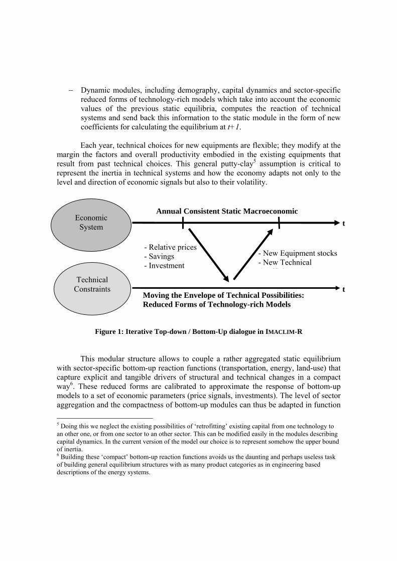
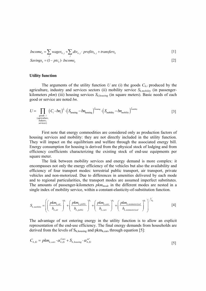
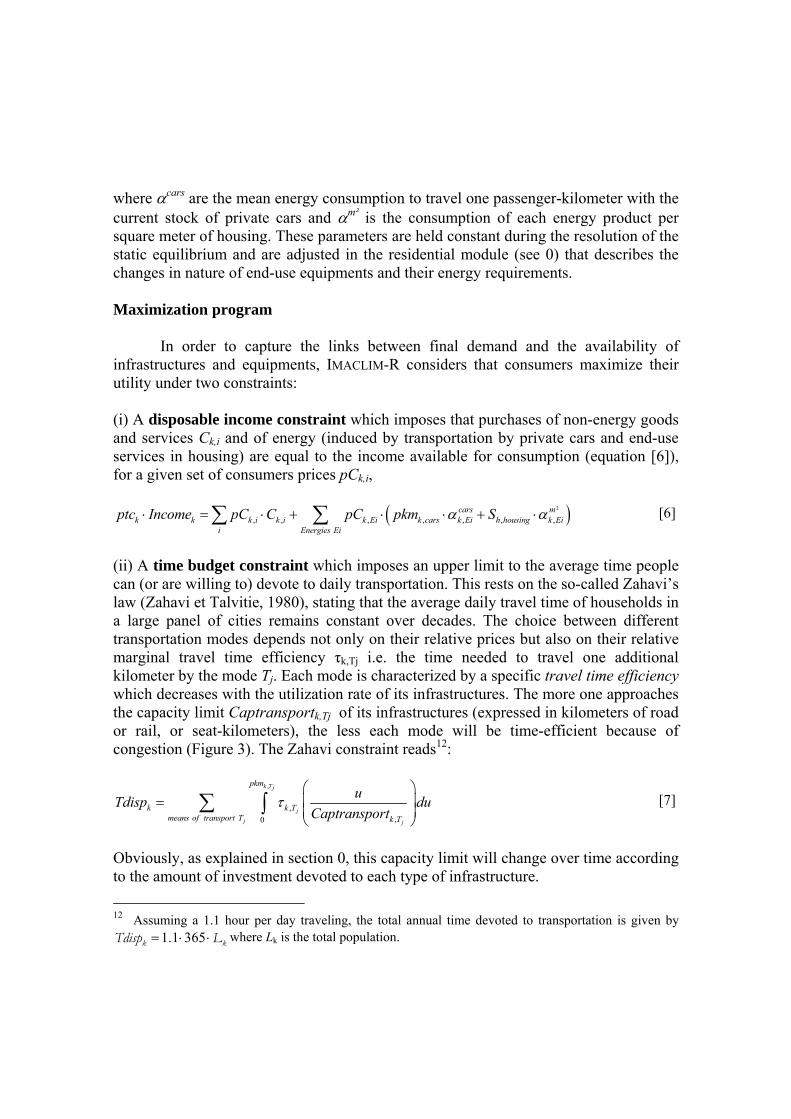
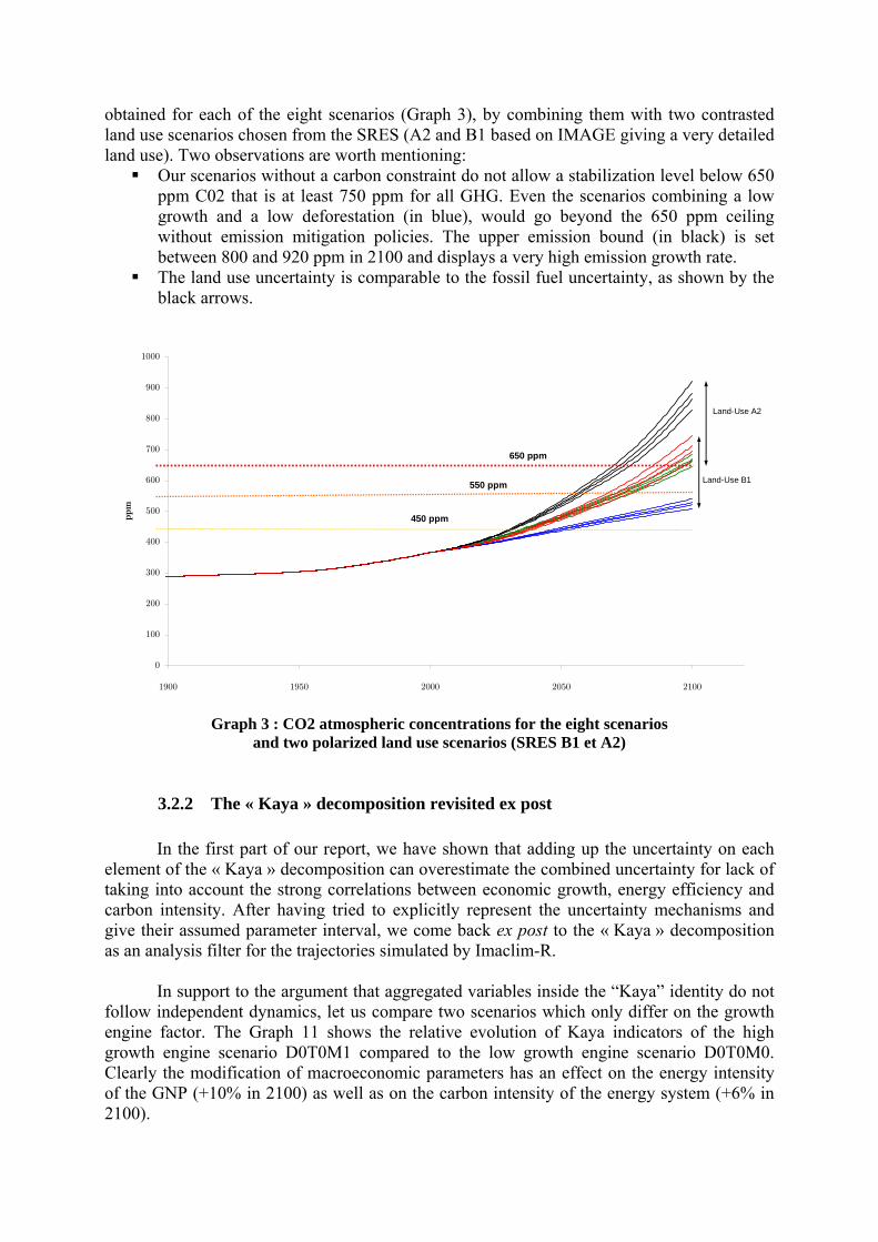
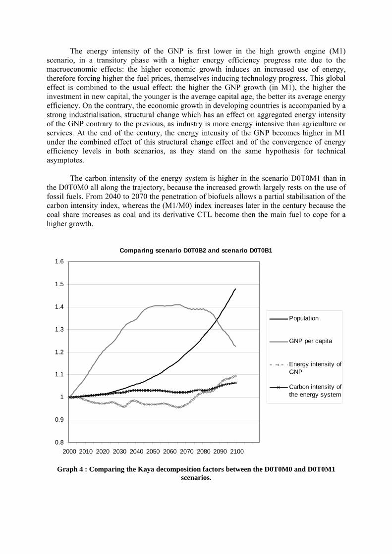
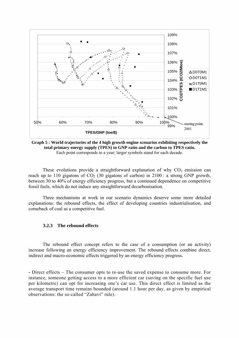
99
100
101
102
103
104
105
106
107
108
109
50 60 70 80 90 100
TPESGNP (toe$)
CO
2TP
ES (t
CO
2M
toe)
D0T0M1D0T1M1D1T0M1D1T1M1
starting point 2001
Graph 5 World trajectories of the 4 high growth engine scenarios exhibiting respectively the
total primary energy supply (TPES) to GNP ratio and the carbon to TPES ratio Each point corresponds to a year larger symbols stand for each decade
These evolutions provide a straightforward explanation of why CO2 emission can reach up to 110 gigatons of CO2 (30 gigatons of carbon) in 2100 a strong GNP growth between 30 to 40 of energy efficiency progress but a continued dependence on competitive fossil fuels which do not induce any straightforward decarbonisation
Three mechanisms at work in our scenario dynamics deserve some more detailed
explanations the rebound effects the effect of developing countries industrialisation and comeback of coal as a competitive fuel
323 The rebound effects
The rebound effect concept refers to the case of a consumption (or an activity) increase following an energy efficiency improvement The rebound effects combine direct indirect and macro-economic effects triggered by an energy efficiency progress
- Direct effects ndash The consumer opts to re-use the saved expense to consume more For instance someone getting access to a more efficient car (saving on the specific fuel use per kilometre) can opt for increasing onersquos car use This direct effect is limited as the average transport time remains bounded (around 11 hour per day as given by empirical observations the so-called ldquoZahavirdquo rule)
- Indirect effects ndash The consumer can opt to re-use the saved expense in consuming more of other goods which in turn induce additional energy consumption For instance a household can save money owing to a more efficient heating system and use it to buy more durable goods for the home equipment - Market effects ndash Less demand for a resource lowers its price which allows marginally more competitive uses For instance the electricity has been initially used for lighting in the residential sector but its decreasing price allowed its use for many other home equipments When talking about emissions the rebound effect corresponds to the difference between the emission reduction projected (by mere transposition of efficiency gains) and the real reduction due to an increased energy efficiency Indeed 30 improvement of energy efficiency wonrsquot lead to 30 reduction of energy expenses nor 30 emissions reduction the difference between these 30 of ldquopotentialrdquo emissions reduction and real reduction is the rebound effect Of course this doesnrsquot mean the rebound effect rules out all benefits of energy efficiency improvements on emissions but it truly limits their impact as we will illustrate with two examples of results given by the model
3231 The rebound effect of the technical progress on the GNP
As the technical progress saves part of the energy expenses for a given energy service
it allows a higher activity level and thus again an increased energy demand which cuts on the initial energy saving
Let us compare for instance D0T0M1 and D0T1M1 scenarios which share the same
development style D0 and the same high growth engine M1 but have different technical progress variant A more rapid technical progress in the D0T0M1 scenario decreases the energy intensity of the GNP for a given date (see Graph 6) However the level of activity represented here by the GNP is higher because of the redeployment of part of the saved energy expenses The net effect on the emission saved is smaller than the gross direct effect The effect is magnified on the carbon budget (ie the cumulated emissions) and therefore on the climate
09
092
094
096
098
1
102
104
2000 2010 2020 2030 2040 2050 2060 2070 2080 2090 2100
Rebound effect onemissions
D0T0M1D0T1M1Carbon budget
D0T0M1D0T1M1Energy intensity ofGNP
D0T0M1D0T1M1GNP per capita
D0T0M1D0T1M1Total emissions
Graph 6 The rebound effect of the technical progress on the GNP and the carbon budget
Comparing the scenarios D0T0M1 and D0T1M1 Index 1 for the scenario D0T1M1
3232 The rebound effect of the technical progress on the mobility
The rebound mechanism described previously has been publicized mostly in the
transport case As explained previously progress in cars efficiency hides partly increases of oil prices and induces more mobility (income effect on the mobility in the householdsrsquo utility function) Additionally to this income effect efficiency improvement can induce changes in the modal shares as the efficiency gains and the weight of energy in the kilometre cost are not homogenous in the different modes The emission reductions expected may thus be counterbalanced partly by mobility increase and modal transfer on more energy intensive transportation modes
Coming back to the comparison between the D0T0M1 and D0T1M1 scenarios which share the same development style D0 and the same high growth engine M1 but are distinguished on the technical progress variant the rebound effect on mobility can be highlighted The trajectories for China (see Graph 7) display more mobility in the more energy efficient scenario (D0T0M1) The total emissions due to cars are the product of the four factors (i) the carbon content of fuels (ii) the specific fuel use per kilometre (energy efficiency of cars) (iii) the mobility per head and (iv) the population (identical for the two scenarios under scrutiny here) The carbon content in the D0T0M1 scenario is slightly higher than in the D0T1M1 scenario because the more efficient route determines a lower cumulated fossil fuel demand and thus lower prices which slows down the entry of bio-fuels Later in the century the efficient route (T0) can still rely on the bio-fuels whereas the less efficient scenario (T1) has saturated the bio-fuel potential and is bound to go more on the coal-to-liquid route
In the end private transport emissions are not mechanically discounted by the ratio of progress on the specific fuel use in the T0 scenario as against the T1 Emissions can even be higher in the transition phase (here from 2025 to 2045) because the higher technical progress is assumed to induce a strong modal shift in favour of the private car option
Results for China
comparing D0T0M1 and D0T1M1
06
07
08
09
1
11
12
2000
2005
2010
2015
2020
2025
2030
2035
2040
2045
2050
2055
2060
2065
2070
2075
2080
2085
2090
2095
Rebound effect onemissions
Carbon budget due tocars
Energy efficiency ofcars
Mobility per capita
Carbon content offuels
Emissions due tocars
Graph 7 The rebound effect of the technical progress on the mobility and the carbon budget
Comparing results for China D0T0M1 compared to D0T1M1 Index 1 is set for the scenario D0T1M1
3233 Effect of the development style on the technical progress
Again the energy technical progress can induce a feedback effect through price in the
case of the development style variant As in the rebound effect case the direct emission difference is partly compensated a less energy intensive development style determines a lower cumulated oil and gas demand and thus a lag in the world price increase In turn it determines less induced technical progress or less induced energy resource substitution for instance towards bio-fuels The projected technical progress penetration effect is reduced as compared to the theoretical energy efficiency gain
This effect is not visible in the Graph 5 because it is negligible as compared to the
energy need difference between both development styles But a detailed D0T1M1 and D1T1M1 comparative analysis can illustrate the compensation mechanism On Graph 8 the D0T1M1 contains less mobility need and thus less oil price increase Therefore it induces less technical progress and a lagged bio-fuels penetration In total the emission projection does not reflect the totality of the gross effect of a lower mobility need determined by a denser space planning
Results for Europe comparing D0T1M1 to D1T1M1
08
085
09
095
1
105
11
2000
2005
2010
2015
2020
2025
2030
2035
2040
2045
2050
2055
2060
2065
2070
2075
2080
2085
2090
2095
Rebound effect onemissions
Carbon budget due tocars
Mobility per capita
Energy efficiency ofcars
Carbon content offuels
Emissions due to cars
Graph 8 The fossil price feedback effect and the carbon budget
The D0T1M1 - D1T1M1 comparison for Europe Index 1 = D1T1M1 scenario
324 The structural change in the developing countries
The CO2 emission per capita in developing countries is much below what it is in industrialized countries even with comparable geographical or climatic areas Therefore the catching-up which is assumed as the central trend of the next century means that the developing countries will be weighting more and more on the world average all along the century Thus we can see on the Graph 5 that the developing countries industrialization catching-up weights as much as to be able to slow down (or even reverse) the global trend of an ever declining global energy intensity into a temporary increase from 2020 to 2040
The Figure 17 illustrates the OECD and non OECD differing trajectories OCDE
countries where the expansion of the service sector is continuous over the whole trajectory see a strong decrease of the energy intensity (around 45 in 2100 as compared to 2000) This decrease of energy intensity goes along with a slow decarbonisation due to progressive penetration of nuclear and renewable energies for electricity generation One should note that these two trajectories presented on the same graph may be misleading the starting point in 2000 represented here by the ratio 100 doesnrsquot correspond to the same absolute values for OECD and non OECD countries The latter remain in our scenarios less efficient than the OECD average Therefore the energy intensity world average will be raised by the growing share taken by non OECD countries in the world GNP (from 20 to 40 between 2000 and 2100 in scenario D1T1M1)
Added Value in Industry
0E+00
5E+06
1E+07
2E+07
2E+07
3E+07
3E+07
4E+07
4E+07
2000 2010 2020 2030 2040 2050 2060 2070 2080 2090
M$
non OECDOECD
Graph 9 OECD and non OECD industry added value in scenario D1T1MI
This effect that we may call laquo aggregation effect raquo is visible when we compare the
world trajectory (as in figure 11) to the regional trajectories (as in figure 17) Beyond the precise data presented here there lies a fundamental issue Will the catching up effect in favour of developing countries share in the world industry (and GNP) be dominated by a leapfrogging effect towards the efficiency frontier or will it still be combined to a strong heritage of the efficiency gap from the starting period In the end the global energy trajectory is differing very significantly The factors bearing on it are as follow the capacity to finance ldquocleanrdquo technologies on productive capital or final equipment the inertia of existing less efficient capital the relative prices of energy compared to domestic prices in developing countries etc
88
93
98
103
108
113
50 60 70 80 90 100
TPESGNP (toe$)
CO2
TPE
S (tC
O2
Mto
e)
OECD
non OECD
Graph 10 OECD and non-OECD trajectories for the scenario D1T1M1
325 The comeback of coal
On the Graph 2 there is a noticeable slow down on the emission growth trajectory beginning around 2035 up to 2065 or 2085 according to the scenario before a steeper slope up to the end of the century This sequence reflects the physical impact of the penetration of bio-fuels from around 2035 on and their saturation between 2065 and 2085 giving room to the coal-to-liquid route This coal comeback is inevitable in a zero carbon price world with a coal-to-liquid technology available and becoming the least cost option It carries a strong risk of an emission explosive trajectory before the end of the century More precisely this ldquocomeback of coalrdquo occurs when remaining oil resources and bio-fuels are not sufficient to satisfy demand for liquid fuels The Imaclim-R model thus does not make the hypothesis of a laquo backstop raquo technology ie a technology apt to penetrate after the price increase gets above its competitive price and then to provide an unlimited supply of a perfect substitute to the exhausted oil reserves and then to the saturated bio-fuels As the existence of such a backstop technology does not seem assured today it seemed to be nor necessary nor robust to make such assumption for our simulations
Liquid fuels
0
20
40
60
80
100
2000
2005
2010
2015
2020
2025
2030
2035
2040
2045
2050
2055
2060
2065
2070
2075
2080
2085
2090
2095
petroleum products
bio-fuels
CTL
Graph 11 The shares of liquid fuels in the scenario D1T1M1
The bio-fuel potential is limited by the land use constraints the competition with food
land allocation and the agricultural yield We have fed into our model the bio-fuel supply potentials as published in the International Energy Agency (IEA 2006) We do not assume a drastic modification of the agricultural system as we are modelling a reference scenario with no carbon policy The bio-fuel global upper limit is nevertheless set at 1400 Mtoe which is about equivalent to the current OPEP oil production Finally the capture and geological sequestration of CO2 would only save the potential emission during the coal-to-liquid process and not the emission which inevitably happens during the engine combustion itself The impact of the comeback of coal on emissions wouldnrsquot be tempered significantly by capture and sequestration
Energy mix Primary Energy
0
20
40
60
80
100
2000
2005
2010
2015
2020
2025
2030
2035
2040
2045
2050
2055
2060
2065
2070
2075
2080
2085
2090
2095
Other renewables
Nuclear
Hydro
Gas
Oil
Coal
Graph 12 The primary energy mix evolution in the D1T1M1 scenario
In the mix of the total primary energy supply the renewable energy share increases
only at a very slow pace whereas the coal remains much more competitive Only the increase
of nuclear in the generation and the shift to electricity of the energy system allows to decrease the fossil energy share in the energy mix as shown Graph 12
326 Impact of growth variants on the fossil content of trajectories The Graph 5 presents the trajectories of the four highest emission scenarios The
impact of moderate growth on laquo Kaya raquo trajectories stems directly from analysis detailed so far Nevertheless we may comment on salient features shown in the Figure 20
The carbon intensity increases by around 4 instead of 8 in the M1 scenarios An energy efficiency quite comparable in 2100 resulting from a slightly lower
technical progress and less rebound effects as well as less industry growth The postponement of the recourse to the coal-to-liquid option in the scenarios with the
ldquosoberrdquo development style variant which benefit from a postponed oil and gas exhaustion
99
100
101
102
103
104
105
50 60 70 80 90 100
TPESGNP (toe$)
CO
2TP
ES (t
CO
2M
toe)
D0T0M0D0T1M0D1T0M0D1T1M0
starting point 2001
Graph 13 Trajectories for 4 scenarios of low growth engine (M0) the energy intensity of GNP
index and the world carbon intensity of energy index Each point represents one year and larger symbols stand for decades
33 Conclusion In this exercice we formulate independent assumptions on the economy growth
engine and on the energy technical progress Therefore the growth impact on the energy efficiency gains is only a second order mechanism through the speed of equipment replacement or the cumulative extraction of fossil resources which in turn have a bearing on the technological package all along the trajectory Nevertheless it widely recognized that the birth the development and the diffusion of innovative technologies are directly correlated to the economic growth for at least two reasons first growth is a precondition to finance the
RampD investments second technical progress may be induced by the anticipations that agents make on the potential gains of expected progress and those anticipations depend notably on the growth rate on the energy price and on the expected fossil reserves Both factors support the interdependence view that the higher the GNP growth expected the higher the technical progress Previous work with an earlier and more compact version of the IMACLIM-R model was especially focused on this topic of induced technical change but not with a perspective of exploring uncertainty
This sounds like a reminder of what was answered by modellers to Castles and Hendersonrsquos criticism against the overestimated growth rates for the catching up of developing countries GNP expressed in current exchange rates Nakicenovic and al (2003) stressed that the emission estimation of SRES was still correct because the effect of overestimated growth rates for developing countries may somehow be compensated by the higher technical progress growth rates as a corollary to the high GNP growth rates McKibbin and al (2004) tested this intuition with the G-Cubed model and showed that emissions are not systematically over-estimated because of higher catching-up growth rates of GNP with the use of market exchange rates
If we lend credibility in the intuition that GNP and technical progress growth rates are correlated we should examine more in depth the assumptions behind the most contrasted scenarios ie D0T0M0 and D1T1M1 to test their self-consistency We cannot decide for sure whether they are still within the uncertainty for crossed intervals on growth and technical progress or whether we miss here a strong link In that case it would mean that the four scenarios (DT1M1 DT0M0) can not be considered as consistent and the most contrasted scenarios would become D0T1M0 and D1T0M1 The initial uncertainty interval between the eight scenarios of 134 to 338 GtC would then decreases to 146-313 GtC that is an interval reduced by 19
4 References Agence Internationale de lrsquoEnergie 2006 ldquoEnergy Technology Perspectives 2006 In support of the G8 Plan of Action Scenarios and Strategies to 2050rdquo pp 283-288 Agence Internationale de lrsquoEnergie 2002 World Energy Oultook Paris 533 p Ch 13 lsquoEnergy and Povertyrsquo Ambrosi P Hourcade J-C Hallegatte S Lecocq F Dumas P Ha Duong M 2003 Optimal control models and elicitation of attitudes towards climate damages Environmental Modeling and Assessment 8 3 133-147 Armington P S 1969 A Theory of Demand for Products Distinguished by Place of Production IMF International Monetary Fund Staff Papers 16 170-201 Berndt E and Wood D 1975 ldquoTechnology Prices and the Derived Demand for Energyrdquo The Review of Economics and Statistics August pp 259-268 Blanchflower D G and A J Oswald 1995 ldquoAn introduction to the Wage Curverdquo Journal of Economic Perspectives 9(3) 153-167 Boumlhringer C Rutherford TF 2005 Integrating Bottom-Up into Top-DownA Mixed Complementarity Approach Discussion Paper No 05-28 ZEW Mannheim 2005 Castles I Henderson D 2003 lsquoThe IPCC Emission Scenarios An Economic-Statistical Critiquersquo Energy amp Environment vol 14 (2-3) pp 159-185 CEPII 2001 Croissance Economique Mondiale un sceacutenario de reacutefeacuterence agrave lrsquohorizon 2030 CEPII working papers Nina Kousnetzoff PARIS deacutecembre 2001 Corrado C and Mattey J 1997 ldquoCapacity Utilizationrdquo Journal of Economic Perspectives Vol 11 No 1 pp 151-167 Crassous R Hourcade J-C Sassi O 2006 Endogenous Structural Change and Climate Targets Modeling experiments with IMACLIM-R The Energy Journal Special Issue lsquoEndogenous Technological Change and the Economics of Atmospheric Stabilisationrsquo 259-276
Criqui P 2001 ldquoPOLES Prospective Outlook on Long-term Energy Systemsrdquo Institut drsquoEacuteconomie et de Politique de lrsquoEacutenergie Grenoble France 9 pp httpwwwupmf-grenoblefriepetextesPOLES8p_01pdf (accessed August 2006) Edmonds JA HM Pitcher RD Sands 2004 Second Generation Model 2004 An Overview httpwwwepagovairpdfsSGMoverviewpdf Frondel M and Schmidt M C 2002 ldquoThe Capital-Energy Controversy An Artifact of Cost Sharesrdquo The Energy Journal Vol23 Issue 3 53-79
Ghersi F Hourcade J-C 2006 Macroeconomic consistency issues in E3 modeling the continued fable of the elephant and the rabbit The Energy Journal 27 (Special Issue ndeg2 Hybrid Modeling of Energ-Environment Policies Reconciling Bottom-up and Top-down) 27-49
Gielen D Kram T Ybema R 1996 ldquoIntegrating Energy and Material Strategies for Greenhouse Gas Reduction A Promising Challengerdquo Change vol 30 June Gitz V 2004 Usage des terres et politiques climatiques globales Thegravese sciences de lenvironnement ENGREF Paris 2004 Hildenbrand W 1994 ldquoMarket Demand theory and empirical evidencerdquo Princeton University Press Hourcade JC 1993 ldquoModelling long-run scenarios Methodology lessons from a prospective study on a low CO2 intensive countryrdquo Energy Policy 21(3) 309-326 Hourcade JC and Ghersi F 2000 Le Rocircle du Changement Technique dans le Double Dividende drsquoEacutecotaxes Eacuteconomie et Preacutevision 143-144 47-68 Hourcade JC Journeacute V 2002 Monsieur Homais les guides de montagne et le maicirctre nageur Variations sur la neacutegation des risques climatiques Critique Internationale 26 pp 65-79 2002 Johansen L 1959 lsquoSubstitution versus Fixed Production Coefficients in the Theory of Growth A synthesisrsquo Econometrica 27 April 1959 157-176 Jorgenson DW and Fraumeini B 1981 ldquoRelative Prices and Technical Changerdquo In ER Berndt and BC Field (eds) Modeling and Measuring Natural Resource Substitution MIT Press Cambridge MA United States Lomborg B 2001 The Skeptical Environmentalist Cambridge University Press 515 pp Maddison A 1995 Monitoring the world economy 1820 ndash 1992 OECD Development Center August 1995 260 p Marshall A 1890 Principles of Economics London Macmillan and Co Ltd 1920 Eighth edition McKibbin W Pearce D Stegman A 2004 lsquoLong-run projections for climate-change scenariosrsquo Brookings Discussion Papers in International Economics No 160 April Washington DC The Brookings Institution
Muellbauer J 1976 ldquoCommunity Preferences and the Representative Consumerrdquo Econometrica 44(5)979-999 Nakicenovic N Gruumlbler A Gaffin S et al 2003 lsquoIPCC SRES revisited a responsersquo Energy amp Environment 14(2-3) May 187-214 Nakicenovic N Alcamo J Davis G de Vries B Fenhann J Gaffin S Gregory K Gruumlbler A Jung TY Kram T La Rovere EL Michaelis L Mori S Morita T Pepper W Pitcher H Price L Riahi K Roehrl A Rogner H-H Sankovski A Schlesinger M Shukla P Smith S Swart R van Rooijen S Victor N Dadi Z 2000 IPCC Special Report on Emissions Scenarios Cambridge University Press Cambridge United Kingdom and New York NY USA 599pp
Oliveira Martins J F Gonand P Antolin C de la Maisonneuve and Kwang-Y 2005 The impact of ageing on demand factor markets and growthrdquo OECD Economics Department Working Papers 420 OECD Economics Department Nordhaus W 2005 Alternative Measures of Output in Global Economic-Environmental ModelsPurchasing Power Parity or Market Exchange Rates Meeting of IPCC Expert Meeting on Emission Scenarios US-EPA Washington DC January 12-14 Rana A Morita T 2000 Scenarios for Greenhouse Gas Emissions A Review of Modeling of Strategies and Policies in Integrated Assessment Models Environmental Economics and Policy Studies 3 (2) 267-289 Rehrl T Friedrich R 2006 Modelling long-term oil price and extraction with a Hubbert approach The LOPEX model Energy Policy 34(15) October 2006 pp 2413-2428 Rivers N and Jaccard M 2005 ldquoCombining Top-Down-Bottom up-Approaches to Energy Economy Modeling Using Discrete Choice Methodsrdquo The Energy Journal 6 (1) 83-106 Schaumlfer A and DG Victor 2000 ldquoThe future mobility of future populationrdquo Transportation Research Part A 34171-205 Solow R 1990 ldquoReactions to Conference Papersrdquo in Diamond P (ed) Growth Productivity Unemployment Essays to Celebrate Bob Solowrsquos Birthday The MIT Press Solow R 1988 ldquoGrowth theory and afterrdquo The American Economic Review 783 307-317 Vuuren D ONeill B 2006 The Consistency of IPCCs SRES Scenarios to 1990ndash2000 Trends and Recent Projections Climatic Change Vol 75 1-2 march 2006 pp 9-46 Weyant et al 1996 ldquoIntegrated Assessment of Climate Change An Overview and Comparison of Approaches and Resultsrdquo in Climate Change 1995 Economic and Social Dimensions of Climate Change JP Bruce H Lee EF Haites (eds) Cambridge University Press Cambridge UK Chapter 10 Sections 101-103 pp 374-380 Zahavi Y and A Talvitie 1980 ldquoRegularities in travel time and money expendituresrdquo Transportation Research Record 750 13plusmn19
- Introduction
- The Imaclim-R framework
-
- Rationale of the Imaclim-R modeling blueprint
-
- A Dual Vision of the Economy an easier dialogue between eng
- A growth engine allowing gaps between potential and real gro
-
- Technical Description
-
- Aggregation scheme and Data
- Static Equilibrium
-
- Households demand of goods services and energy
- Production constraints and supply curves
- Governments
- Labor market
- Capital flows and investments
- Goodsrsquo markets and international trade
- Equilibrium constraints on physical flows
- Choice of a numeraire
- Greenhouse gas emissions
-
- Dynamic Linkages Growth engine and technical change
-
- The growth engine demography productivity and investment
- Energy-related technical change
-
- Supply of energy
- Demand of Energy
-
- Long-run emission scenarios
-
- Assumptions
-
- The growth engine
-
- Demography transition slow vs rapid and extended
- Labour productivity North American leadership but a variant
-
- Development styles laquo energy intensive raquo vs laquo energy sober raquo
- Energy and technology variables variants on technical progr
- Eight alternative scenarios
-
- Emission scenarios
-
- What risks of a high carbon future
- The laquo Kaya raquo decomposition revisited ex post
- The rebound effects
-
- The rebound effect of the technical progress on the GNP
- The rebound effect of the technical progress on the mobility
- Effect of the development style on the technical progress
-
- The structural change in the developing countries
- The comeback of coal
- Impact of growth variants on the fossil content of trajector
-
- Conclusion
-
- References
-
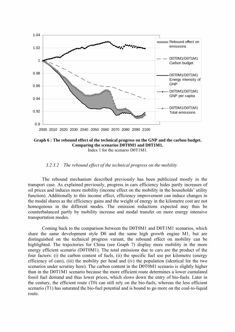
09
092
094
096
098
1
102
104
2000 2010 2020 2030 2040 2050 2060 2070 2080 2090 2100
Rebound effect onemissions
D0T0M1D0T1M1Carbon budget
D0T0M1D0T1M1Energy intensity ofGNP
D0T0M1D0T1M1GNP per capita
D0T0M1D0T1M1Total emissions
Graph 6 The rebound effect of the technical progress on the GNP and the carbon budget
Comparing the scenarios D0T0M1 and D0T1M1 Index 1 for the scenario D0T1M1
3232 The rebound effect of the technical progress on the mobility
The rebound mechanism described previously has been publicized mostly in the
transport case As explained previously progress in cars efficiency hides partly increases of oil prices and induces more mobility (income effect on the mobility in the householdsrsquo utility function) Additionally to this income effect efficiency improvement can induce changes in the modal shares as the efficiency gains and the weight of energy in the kilometre cost are not homogenous in the different modes The emission reductions expected may thus be counterbalanced partly by mobility increase and modal transfer on more energy intensive transportation modes
Coming back to the comparison between the D0T0M1 and D0T1M1 scenarios which share the same development style D0 and the same high growth engine M1 but are distinguished on the technical progress variant the rebound effect on mobility can be highlighted The trajectories for China (see Graph 7) display more mobility in the more energy efficient scenario (D0T0M1) The total emissions due to cars are the product of the four factors (i) the carbon content of fuels (ii) the specific fuel use per kilometre (energy efficiency of cars) (iii) the mobility per head and (iv) the population (identical for the two scenarios under scrutiny here) The carbon content in the D0T0M1 scenario is slightly higher than in the D0T1M1 scenario because the more efficient route determines a lower cumulated fossil fuel demand and thus lower prices which slows down the entry of bio-fuels Later in the century the efficient route (T0) can still rely on the bio-fuels whereas the less efficient scenario (T1) has saturated the bio-fuel potential and is bound to go more on the coal-to-liquid route
In the end private transport emissions are not mechanically discounted by the ratio of progress on the specific fuel use in the T0 scenario as against the T1 Emissions can even be higher in the transition phase (here from 2025 to 2045) because the higher technical progress is assumed to induce a strong modal shift in favour of the private car option
Results for China
comparing D0T0M1 and D0T1M1
06
07
08
09
1
11
12
2000
2005
2010
2015
2020
2025
2030
2035
2040
2045
2050
2055
2060
2065
2070
2075
2080
2085
2090
2095
Rebound effect onemissions
Carbon budget due tocars
Energy efficiency ofcars
Mobility per capita
Carbon content offuels
Emissions due tocars
Graph 7 The rebound effect of the technical progress on the mobility and the carbon budget
Comparing results for China D0T0M1 compared to D0T1M1 Index 1 is set for the scenario D0T1M1
3233 Effect of the development style on the technical progress
Again the energy technical progress can induce a feedback effect through price in the
case of the development style variant As in the rebound effect case the direct emission difference is partly compensated a less energy intensive development style determines a lower cumulated oil and gas demand and thus a lag in the world price increase In turn it determines less induced technical progress or less induced energy resource substitution for instance towards bio-fuels The projected technical progress penetration effect is reduced as compared to the theoretical energy efficiency gain
This effect is not visible in the Graph 5 because it is negligible as compared to the
energy need difference between both development styles But a detailed D0T1M1 and D1T1M1 comparative analysis can illustrate the compensation mechanism On Graph 8 the D0T1M1 contains less mobility need and thus less oil price increase Therefore it induces less technical progress and a lagged bio-fuels penetration In total the emission projection does not reflect the totality of the gross effect of a lower mobility need determined by a denser space planning
Results for Europe comparing D0T1M1 to D1T1M1
08
085
09
095
1
105
11
2000
2005
2010
2015
2020
2025
2030
2035
2040
2045
2050
2055
2060
2065
2070
2075
2080
2085
2090
2095
Rebound effect onemissions
Carbon budget due tocars
Mobility per capita
Energy efficiency ofcars
Carbon content offuels
Emissions due to cars
Graph 8 The fossil price feedback effect and the carbon budget
The D0T1M1 - D1T1M1 comparison for Europe Index 1 = D1T1M1 scenario
324 The structural change in the developing countries
The CO2 emission per capita in developing countries is much below what it is in industrialized countries even with comparable geographical or climatic areas Therefore the catching-up which is assumed as the central trend of the next century means that the developing countries will be weighting more and more on the world average all along the century Thus we can see on the Graph 5 that the developing countries industrialization catching-up weights as much as to be able to slow down (or even reverse) the global trend of an ever declining global energy intensity into a temporary increase from 2020 to 2040
The Figure 17 illustrates the OECD and non OECD differing trajectories OCDE
countries where the expansion of the service sector is continuous over the whole trajectory see a strong decrease of the energy intensity (around 45 in 2100 as compared to 2000) This decrease of energy intensity goes along with a slow decarbonisation due to progressive penetration of nuclear and renewable energies for electricity generation One should note that these two trajectories presented on the same graph may be misleading the starting point in 2000 represented here by the ratio 100 doesnrsquot correspond to the same absolute values for OECD and non OECD countries The latter remain in our scenarios less efficient than the OECD average Therefore the energy intensity world average will be raised by the growing share taken by non OECD countries in the world GNP (from 20 to 40 between 2000 and 2100 in scenario D1T1M1)
Added Value in Industry
0E+00
5E+06
1E+07
2E+07
2E+07
3E+07
3E+07
4E+07
4E+07
2000 2010 2020 2030 2040 2050 2060 2070 2080 2090
M$
non OECDOECD
Graph 9 OECD and non OECD industry added value in scenario D1T1MI
This effect that we may call laquo aggregation effect raquo is visible when we compare the
world trajectory (as in figure 11) to the regional trajectories (as in figure 17) Beyond the precise data presented here there lies a fundamental issue Will the catching up effect in favour of developing countries share in the world industry (and GNP) be dominated by a leapfrogging effect towards the efficiency frontier or will it still be combined to a strong heritage of the efficiency gap from the starting period In the end the global energy trajectory is differing very significantly The factors bearing on it are as follow the capacity to finance ldquocleanrdquo technologies on productive capital or final equipment the inertia of existing less efficient capital the relative prices of energy compared to domestic prices in developing countries etc
88
93
98
103
108
113
50 60 70 80 90 100
TPESGNP (toe$)
CO2
TPE
S (tC
O2
Mto
e)
OECD
non OECD
Graph 10 OECD and non-OECD trajectories for the scenario D1T1M1
325 The comeback of coal
On the Graph 2 there is a noticeable slow down on the emission growth trajectory beginning around 2035 up to 2065 or 2085 according to the scenario before a steeper slope up to the end of the century This sequence reflects the physical impact of the penetration of bio-fuels from around 2035 on and their saturation between 2065 and 2085 giving room to the coal-to-liquid route This coal comeback is inevitable in a zero carbon price world with a coal-to-liquid technology available and becoming the least cost option It carries a strong risk of an emission explosive trajectory before the end of the century More precisely this ldquocomeback of coalrdquo occurs when remaining oil resources and bio-fuels are not sufficient to satisfy demand for liquid fuels The Imaclim-R model thus does not make the hypothesis of a laquo backstop raquo technology ie a technology apt to penetrate after the price increase gets above its competitive price and then to provide an unlimited supply of a perfect substitute to the exhausted oil reserves and then to the saturated bio-fuels As the existence of such a backstop technology does not seem assured today it seemed to be nor necessary nor robust to make such assumption for our simulations
Liquid fuels
0
20
40
60
80
100
2000
2005
2010
2015
2020
2025
2030
2035
2040
2045
2050
2055
2060
2065
2070
2075
2080
2085
2090
2095
petroleum products
bio-fuels
CTL
Graph 11 The shares of liquid fuels in the scenario D1T1M1
The bio-fuel potential is limited by the land use constraints the competition with food
land allocation and the agricultural yield We have fed into our model the bio-fuel supply potentials as published in the International Energy Agency (IEA 2006) We do not assume a drastic modification of the agricultural system as we are modelling a reference scenario with no carbon policy The bio-fuel global upper limit is nevertheless set at 1400 Mtoe which is about equivalent to the current OPEP oil production Finally the capture and geological sequestration of CO2 would only save the potential emission during the coal-to-liquid process and not the emission which inevitably happens during the engine combustion itself The impact of the comeback of coal on emissions wouldnrsquot be tempered significantly by capture and sequestration
Energy mix Primary Energy
0
20
40
60
80
100
2000
2005
2010
2015
2020
2025
2030
2035
2040
2045
2050
2055
2060
2065
2070
2075
2080
2085
2090
2095
Other renewables
Nuclear
Hydro
Gas
Oil
Coal
Graph 12 The primary energy mix evolution in the D1T1M1 scenario
In the mix of the total primary energy supply the renewable energy share increases
only at a very slow pace whereas the coal remains much more competitive Only the increase
of nuclear in the generation and the shift to electricity of the energy system allows to decrease the fossil energy share in the energy mix as shown Graph 12
326 Impact of growth variants on the fossil content of trajectories The Graph 5 presents the trajectories of the four highest emission scenarios The
impact of moderate growth on laquo Kaya raquo trajectories stems directly from analysis detailed so far Nevertheless we may comment on salient features shown in the Figure 20
The carbon intensity increases by around 4 instead of 8 in the M1 scenarios An energy efficiency quite comparable in 2100 resulting from a slightly lower
technical progress and less rebound effects as well as less industry growth The postponement of the recourse to the coal-to-liquid option in the scenarios with the
ldquosoberrdquo development style variant which benefit from a postponed oil and gas exhaustion
99
100
101
102
103
104
105
50 60 70 80 90 100
TPESGNP (toe$)
CO
2TP
ES (t
CO
2M
toe)
D0T0M0D0T1M0D1T0M0D1T1M0
starting point 2001
Graph 13 Trajectories for 4 scenarios of low growth engine (M0) the energy intensity of GNP
index and the world carbon intensity of energy index Each point represents one year and larger symbols stand for decades
33 Conclusion In this exercice we formulate independent assumptions on the economy growth
engine and on the energy technical progress Therefore the growth impact on the energy efficiency gains is only a second order mechanism through the speed of equipment replacement or the cumulative extraction of fossil resources which in turn have a bearing on the technological package all along the trajectory Nevertheless it widely recognized that the birth the development and the diffusion of innovative technologies are directly correlated to the economic growth for at least two reasons first growth is a precondition to finance the
RampD investments second technical progress may be induced by the anticipations that agents make on the potential gains of expected progress and those anticipations depend notably on the growth rate on the energy price and on the expected fossil reserves Both factors support the interdependence view that the higher the GNP growth expected the higher the technical progress Previous work with an earlier and more compact version of the IMACLIM-R model was especially focused on this topic of induced technical change but not with a perspective of exploring uncertainty
This sounds like a reminder of what was answered by modellers to Castles and Hendersonrsquos criticism against the overestimated growth rates for the catching up of developing countries GNP expressed in current exchange rates Nakicenovic and al (2003) stressed that the emission estimation of SRES was still correct because the effect of overestimated growth rates for developing countries may somehow be compensated by the higher technical progress growth rates as a corollary to the high GNP growth rates McKibbin and al (2004) tested this intuition with the G-Cubed model and showed that emissions are not systematically over-estimated because of higher catching-up growth rates of GNP with the use of market exchange rates
If we lend credibility in the intuition that GNP and technical progress growth rates are correlated we should examine more in depth the assumptions behind the most contrasted scenarios ie D0T0M0 and D1T1M1 to test their self-consistency We cannot decide for sure whether they are still within the uncertainty for crossed intervals on growth and technical progress or whether we miss here a strong link In that case it would mean that the four scenarios (DT1M1 DT0M0) can not be considered as consistent and the most contrasted scenarios would become D0T1M0 and D1T0M1 The initial uncertainty interval between the eight scenarios of 134 to 338 GtC would then decreases to 146-313 GtC that is an interval reduced by 19
4 References Agence Internationale de lrsquoEnergie 2006 ldquoEnergy Technology Perspectives 2006 In support of the G8 Plan of Action Scenarios and Strategies to 2050rdquo pp 283-288 Agence Internationale de lrsquoEnergie 2002 World Energy Oultook Paris 533 p Ch 13 lsquoEnergy and Povertyrsquo Ambrosi P Hourcade J-C Hallegatte S Lecocq F Dumas P Ha Duong M 2003 Optimal control models and elicitation of attitudes towards climate damages Environmental Modeling and Assessment 8 3 133-147 Armington P S 1969 A Theory of Demand for Products Distinguished by Place of Production IMF International Monetary Fund Staff Papers 16 170-201 Berndt E and Wood D 1975 ldquoTechnology Prices and the Derived Demand for Energyrdquo The Review of Economics and Statistics August pp 259-268 Blanchflower D G and A J Oswald 1995 ldquoAn introduction to the Wage Curverdquo Journal of Economic Perspectives 9(3) 153-167 Boumlhringer C Rutherford TF 2005 Integrating Bottom-Up into Top-DownA Mixed Complementarity Approach Discussion Paper No 05-28 ZEW Mannheim 2005 Castles I Henderson D 2003 lsquoThe IPCC Emission Scenarios An Economic-Statistical Critiquersquo Energy amp Environment vol 14 (2-3) pp 159-185 CEPII 2001 Croissance Economique Mondiale un sceacutenario de reacutefeacuterence agrave lrsquohorizon 2030 CEPII working papers Nina Kousnetzoff PARIS deacutecembre 2001 Corrado C and Mattey J 1997 ldquoCapacity Utilizationrdquo Journal of Economic Perspectives Vol 11 No 1 pp 151-167 Crassous R Hourcade J-C Sassi O 2006 Endogenous Structural Change and Climate Targets Modeling experiments with IMACLIM-R The Energy Journal Special Issue lsquoEndogenous Technological Change and the Economics of Atmospheric Stabilisationrsquo 259-276
Criqui P 2001 ldquoPOLES Prospective Outlook on Long-term Energy Systemsrdquo Institut drsquoEacuteconomie et de Politique de lrsquoEacutenergie Grenoble France 9 pp httpwwwupmf-grenoblefriepetextesPOLES8p_01pdf (accessed August 2006) Edmonds JA HM Pitcher RD Sands 2004 Second Generation Model 2004 An Overview httpwwwepagovairpdfsSGMoverviewpdf Frondel M and Schmidt M C 2002 ldquoThe Capital-Energy Controversy An Artifact of Cost Sharesrdquo The Energy Journal Vol23 Issue 3 53-79
Ghersi F Hourcade J-C 2006 Macroeconomic consistency issues in E3 modeling the continued fable of the elephant and the rabbit The Energy Journal 27 (Special Issue ndeg2 Hybrid Modeling of Energ-Environment Policies Reconciling Bottom-up and Top-down) 27-49
Gielen D Kram T Ybema R 1996 ldquoIntegrating Energy and Material Strategies for Greenhouse Gas Reduction A Promising Challengerdquo Change vol 30 June Gitz V 2004 Usage des terres et politiques climatiques globales Thegravese sciences de lenvironnement ENGREF Paris 2004 Hildenbrand W 1994 ldquoMarket Demand theory and empirical evidencerdquo Princeton University Press Hourcade JC 1993 ldquoModelling long-run scenarios Methodology lessons from a prospective study on a low CO2 intensive countryrdquo Energy Policy 21(3) 309-326 Hourcade JC and Ghersi F 2000 Le Rocircle du Changement Technique dans le Double Dividende drsquoEacutecotaxes Eacuteconomie et Preacutevision 143-144 47-68 Hourcade JC Journeacute V 2002 Monsieur Homais les guides de montagne et le maicirctre nageur Variations sur la neacutegation des risques climatiques Critique Internationale 26 pp 65-79 2002 Johansen L 1959 lsquoSubstitution versus Fixed Production Coefficients in the Theory of Growth A synthesisrsquo Econometrica 27 April 1959 157-176 Jorgenson DW and Fraumeini B 1981 ldquoRelative Prices and Technical Changerdquo In ER Berndt and BC Field (eds) Modeling and Measuring Natural Resource Substitution MIT Press Cambridge MA United States Lomborg B 2001 The Skeptical Environmentalist Cambridge University Press 515 pp Maddison A 1995 Monitoring the world economy 1820 ndash 1992 OECD Development Center August 1995 260 p Marshall A 1890 Principles of Economics London Macmillan and Co Ltd 1920 Eighth edition McKibbin W Pearce D Stegman A 2004 lsquoLong-run projections for climate-change scenariosrsquo Brookings Discussion Papers in International Economics No 160 April Washington DC The Brookings Institution
Muellbauer J 1976 ldquoCommunity Preferences and the Representative Consumerrdquo Econometrica 44(5)979-999 Nakicenovic N Gruumlbler A Gaffin S et al 2003 lsquoIPCC SRES revisited a responsersquo Energy amp Environment 14(2-3) May 187-214 Nakicenovic N Alcamo J Davis G de Vries B Fenhann J Gaffin S Gregory K Gruumlbler A Jung TY Kram T La Rovere EL Michaelis L Mori S Morita T Pepper W Pitcher H Price L Riahi K Roehrl A Rogner H-H Sankovski A Schlesinger M Shukla P Smith S Swart R van Rooijen S Victor N Dadi Z 2000 IPCC Special Report on Emissions Scenarios Cambridge University Press Cambridge United Kingdom and New York NY USA 599pp
Oliveira Martins J F Gonand P Antolin C de la Maisonneuve and Kwang-Y 2005 The impact of ageing on demand factor markets and growthrdquo OECD Economics Department Working Papers 420 OECD Economics Department Nordhaus W 2005 Alternative Measures of Output in Global Economic-Environmental ModelsPurchasing Power Parity or Market Exchange Rates Meeting of IPCC Expert Meeting on Emission Scenarios US-EPA Washington DC January 12-14 Rana A Morita T 2000 Scenarios for Greenhouse Gas Emissions A Review of Modeling of Strategies and Policies in Integrated Assessment Models Environmental Economics and Policy Studies 3 (2) 267-289 Rehrl T Friedrich R 2006 Modelling long-term oil price and extraction with a Hubbert approach The LOPEX model Energy Policy 34(15) October 2006 pp 2413-2428 Rivers N and Jaccard M 2005 ldquoCombining Top-Down-Bottom up-Approaches to Energy Economy Modeling Using Discrete Choice Methodsrdquo The Energy Journal 6 (1) 83-106 Schaumlfer A and DG Victor 2000 ldquoThe future mobility of future populationrdquo Transportation Research Part A 34171-205 Solow R 1990 ldquoReactions to Conference Papersrdquo in Diamond P (ed) Growth Productivity Unemployment Essays to Celebrate Bob Solowrsquos Birthday The MIT Press Solow R 1988 ldquoGrowth theory and afterrdquo The American Economic Review 783 307-317 Vuuren D ONeill B 2006 The Consistency of IPCCs SRES Scenarios to 1990ndash2000 Trends and Recent Projections Climatic Change Vol 75 1-2 march 2006 pp 9-46 Weyant et al 1996 ldquoIntegrated Assessment of Climate Change An Overview and Comparison of Approaches and Resultsrdquo in Climate Change 1995 Economic and Social Dimensions of Climate Change JP Bruce H Lee EF Haites (eds) Cambridge University Press Cambridge UK Chapter 10 Sections 101-103 pp 374-380 Zahavi Y and A Talvitie 1980 ldquoRegularities in travel time and money expendituresrdquo Transportation Research Record 750 13plusmn19
- Introduction
- The Imaclim-R framework
-
- Rationale of the Imaclim-R modeling blueprint
-
- A Dual Vision of the Economy an easier dialogue between eng
- A growth engine allowing gaps between potential and real gro
-
- Technical Description
-
- Aggregation scheme and Data
- Static Equilibrium
-
- Households demand of goods services and energy
- Production constraints and supply curves
- Governments
- Labor market
- Capital flows and investments
- Goodsrsquo markets and international trade
- Equilibrium constraints on physical flows
- Choice of a numeraire
- Greenhouse gas emissions
-
- Dynamic Linkages Growth engine and technical change
-
- The growth engine demography productivity and investment
- Energy-related technical change
-
- Supply of energy
- Demand of Energy
-
- Long-run emission scenarios
-
- Assumptions
-
- The growth engine
-
- Demography transition slow vs rapid and extended
- Labour productivity North American leadership but a variant
-
- Development styles laquo energy intensive raquo vs laquo energy sober raquo
- Energy and technology variables variants on technical progr
- Eight alternative scenarios
-
- Emission scenarios
-
- What risks of a high carbon future
- The laquo Kaya raquo decomposition revisited ex post
- The rebound effects
-
- The rebound effect of the technical progress on the GNP
- The rebound effect of the technical progress on the mobility
- Effect of the development style on the technical progress
-
- The structural change in the developing countries
- The comeback of coal
- Impact of growth variants on the fossil content of trajector
-
- Conclusion
-
- References
-
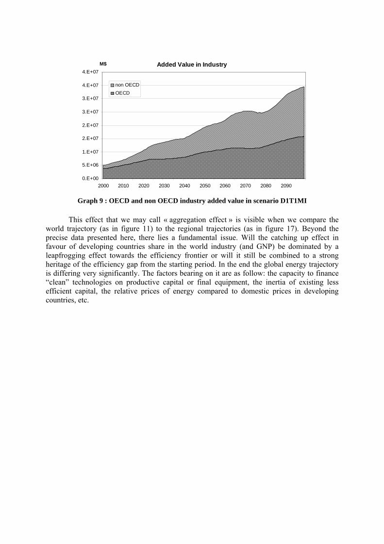
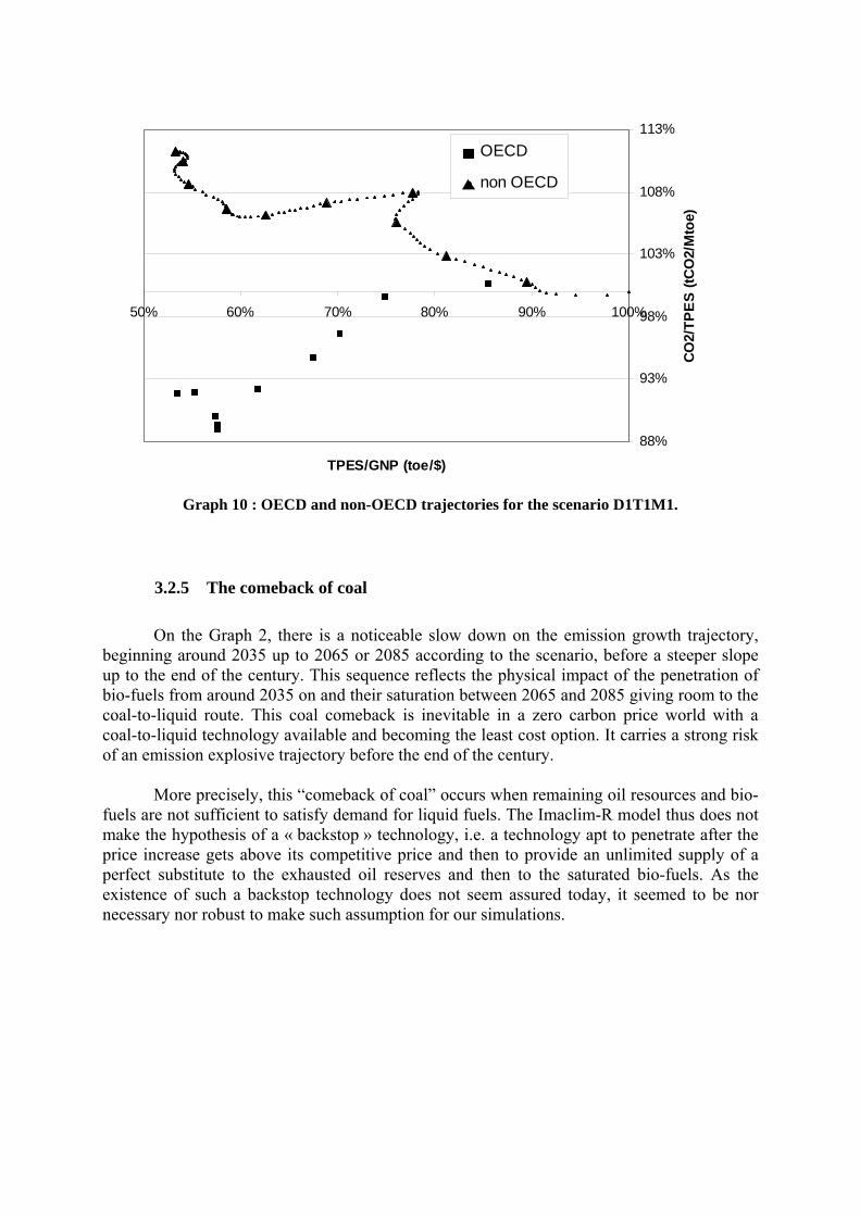