exploiting wi-fi channel state information for artificial
TRANSCRIPT

Exploiting Wi-Fi Channel State Information for
Artificial Intelligence-Based Human Activity
Recognition of Similar Dynamic Motions
by
Itaf Omar Joudeh
A thesis submitted to the Faculty of Graduate and Postdoctoral
Affairs in partial fulfillment of the requirements for the degree of
Master of Applied Science
in
Electrical and Computer Engineering (Data Science)
Carleton University
Ottawa, Ontario
© 2020, Itaf Omar Joudeh

ii
Copyright
Parts of this thesis come from [1], “WiFi Channel State Information-Based Recognition of
Sitting-Down and Standing-Up Activities,” a conference proceedings paper, published by
the Institute of Electrical and Electronics Engineers (IEEE). The IEEE does not require
individuals working on a thesis to obtain a formal reuse license, however, in the text,
material from this source will be identified as © 2019 [1], accordingly.

iii
Abstract
Real-time recognition of Activities of Daily Living (ADLs) enables surveillance, security,
and health monitoring applications. Establishing systems to recognize ADLs non-
intrusively and passively, would facilitate smart spaces by providing assistive living for
seniors and people with disabilities. This work applies artificial intelligence to pervasive
Wi-Fi technology to measure motion and distinguish the patterns associated with dynamic
activities. Processed signals are segmented into labelled sequences. Statistical features are
extracted to enable activity recognition. Classifiers are tested to predict activities. Support
vector machines achieve the best performance at distinguishing still, sitting-down, and
standing-up activity classes. Results on data collected by one subject achieve a
classification accuracy of 98.8% for sitting and standing activities at one room location,
within one experimental setup, and 98.5% for various activity locations, within different
experimental setups. Results on data collected by four subjects achieve an accuracy of
97.6% for sitting and standing activities at random room locations.

iv
Acknowledgements
This study was partially funded by a Discovery Grant and an Engage Grant from the
Natural Sciences and Engineering Research Council (NSERC) of Canada, and was
performed in collaboration with Aerial Technologies, Inc.
I would like to thank all members of my family, one by one, for their continued,
unconditional love and support. I love them more than anything in this whole world!
Also, I would like to thank my supervisors, Dr. Cretu, Dr. Wallace, and Dr. Goubran, for
their time and assistance. I would like to acknowledge my medical advisor, Dr. Knoefel,
for being responsive and available. It was a great pleasure to work with them!
Nonetheless, I would also like to acknowledge my colleagues in the DSP lab at Carleton
University, for all their help in performing some experiments. I enjoyed working with such
nice people!
Last but not least, I really appreciate the services provided by the technical staff in the
Department of Systems and Computer Engineering (SCE) at Carleton University.

v
Table of Contents
Copyright ........................................................................................................................... ii
Abstract ............................................................................................................................. iii
Acknowledgements .......................................................................................................... iv
Table of Contents .............................................................................................................. v
List of Tables .................................................................................................................... ix
List of Figures ................................................................................................................. xiii
List of Appendices .......................................................................................................... xvi
Table of Acronyms ........................................................................................................ xvii
Chapter 1: Introduction .................................................................................................. 1
1.1 Motivation ........................................................................................................... 1
1.2 Objectives ........................................................................................................... 1
1.3 Problem Statement .............................................................................................. 2
1.4 Contributions....................................................................................................... 2
1.5 Thesis Structure .................................................................................................. 4
Chapter 2: Background ................................................................................................... 5
2.1 Activities of Daily Living (ADLs) ...................................................................... 5
2.2 ADL Assessment Technologies .......................................................................... 6
2.2.1 Usability of ADL Sensing Options for Aging Adults ........................................ 6
2.2.2 ADL Assessment with Cameras ......................................................................... 7
2.2.3 ADL Assessment with Sensors and Smartphones .............................................. 8
2.2.4 ADL Assessment with Radar ........................................................................... 10
2.2.5 ADL Assessment with Wi-Fi ........................................................................... 10
vi
2.3 Machine Learning ............................................................................................. 13
2.3.1 Training ............................................................................................................ 14
2.3.2 Testing and Validation ..................................................................................... 15
2.3.3 Performance Metrics ........................................................................................ 16
2.4 Deep Learning ................................................................................................... 17
Chapter 3: Equipment ................................................................................................... 19
3.1 Theory of Operation of the Equipment ............................................................. 19
3.2 Working Principle of the Equipment ................................................................ 20
3.3 Deployment of the Equipment .......................................................................... 21
Chapter 4: Proposed Solution ....................................................................................... 23
4.1 Data Collection ................................................................................................. 24
4.2 Data Preprocessing............................................................................................ 25
4.3 Feature Extraction and Selection ...................................................................... 27
4.4 Class Imbalance ................................................................................................ 31
4.5 Classification..................................................................................................... 32
4.5.1 Classification via Traditional Machine Learning ............................................. 32
4.5.2 Classification via Deep Learning ..................................................................... 35
Chapter 5: Experimental Results ................................................................................. 38
5.1 Distinguishing Sitting-down and Standing-up Activities ................................. 38
5.1.1 Preliminary Sitting and Standing Experiments by One Subject....................... 38
5.1.2 Preliminary Results .......................................................................................... 40
5.2 Pre-processing Techniques ............................................................................... 42
5.2.1 Experiments with Data Preprocessing Techniques .......................................... 43
5.2.2 CSI Normalization ............................................................................................ 44

vii
5.2.3 Feature Scaling ................................................................................................. 44
5.2.4. Optimization of Preprocessing Methodology ................................................. 46
5.3 Subject Activity and Device Location Independence ....................................... 48
5.3.1 Experiments on Activity Location Independence ............................................ 48
5.3.2 Independence of Activity Location .................................................................. 52
5.3.3 Independence of Device Location .................................................................... 54
5.4 Time Repeatability and Drift ............................................................................ 59
5.4.1 Experiments over Time .................................................................................... 59
5.4.2 Time Repeatability and Independence ............................................................. 60
5.4.3 Signal Drift ....................................................................................................... 66
5.5 Testing and Validation on More Subjects ......................................................... 70
5.5.1 Experiments by Other Subjects ........................................................................ 70
5.5.2 Dependence of Classification Performance on Subjects .................................. 71
5.5.3 Independence of Classification Performance from Subjects ............................ 74
5.5.4 Deep Learning Results ..................................................................................... 80
5.5.4.1 Sequence-to-Sequence BiLSTM Network ............................................ 81
5.5.4.2 Sequence-to-Label BiLSTM Network .................................................. 81
Chapter 6: Conclusion ................................................................................................... 84
6.1 Summary of Related Work ............................................................................... 84
6.2 Discussion of Results ........................................................................................ 85
6.3 Future Work ...................................................................................................... 89
Appendices ....................................................................................................................... 91
Appendix A Summary of Data Samples ....................................................................... 91
Appendix B Samples of Preprocessed Data .................................................................. 94
viii
B.1 Raw Signal ....................................................................................................... 94
B.2 Filtering ............................................................................................................ 95
B.3 Normalization ................................................................................................... 96
B.4 Feature Scaling ............................................................................................... 100
B.5 Filtering, Z-Score Standardization, and Feature Scaling Combined .............. 103
Appendix C Samples of Data from Different Activity Locations .............................. 104
C.1 Middle ............................................................................................................ 104
C.2 Near the Transmitter ....................................................................................... 105
C.3 Near the Receiver ........................................................................................... 106
C.4 Empty Corners ................................................................................................ 107
Appendix D Samples of Data with Different Device Placements .............................. 109
D.1 2D (Ground-Ground) Device Placement ........................................................ 109
D.2 3D (Ceiling-Ground) Device Placement ........................................................ 110
Appendix E Samples of Data by Different Subjects ................................................... 111
E.1 Subject 1 (I) .................................................................................................... 111
E.2 Subject 2 (M) .................................................................................................. 112
E.3 Subject 3 (J) .................................................................................................... 113
E.4 Subject 4 (H) .................................................................................................. 114
Bibliography or References .......................................................................................... 115

ix
List of Tables
Table 1 Cameras vs. Sensors vs. Wi-Fi vs. Radar ........................................................... 7
Table 2 Preliminary Classification Results .................................................................... 41
Table 3 Confusion Matrix of the Medium Gaussian SVM for the “preliminary” Data
Set ..................................................................................................................................... 42
Table 4 Comparison of Classification Accuracies achieved by Normalization
Approaches ....................................................................................................................... 45
Table 5 Comparison of Classification Accuracies achieved by Feature Scaling
Approaches ....................................................................................................................... 46
Table 6 Classification Results with Optimum Preprocessing Methodology ................. 47
Table 7 Summary of Test Scenarios .............................................................................. 51
Table 8 Classification Results Demonstrating the Independence of Performance with
Respect to Activity Location ............................................................................................ 53
Table 9 Device Placement Classification Results .......................................................... 55
Table 10 Confusion Matrix of the Medium Gaussian SVM for the “preliminary” Data
Set ..................................................................................................................................... 57
Table 11 Confusion Matrix of the Medium Gaussian SVM for the “floor” Data Set ... 57
Table 12 Confusion Matrix of the Medium Gaussian SVM for the “ceiling” Data Set 58
Table 13 Confusion Matrix of the Medium Gaussian SVM for the “floor + ceiling”
Data Set ............................................................................................................................. 58
Table 14 Classification Results for Time Repeatability Evaluation .............................. 62

x
Table 15 Confusion Matrix Summarizing the Medium Gaussian SVM Predictions for
“day 1” .............................................................................................................................. 63
Table 16 Confusion Matrix Summarizing the Medium Gaussian SVM Predictions for
“day 2” .............................................................................................................................. 63
Table 17 Classification Results showing Time Repeatability on Two Data Sets from the
Same Day .......................................................................................................................... 64
Table 18 Confusion Matrix Summarizing the Medium Gaussian SVM Predictions for
Capture 1 ........................................................................................................................... 65
Table 19 Confusion Matrix Summarizing the Medium Gaussian SVM Predictions for
Capture 2 ........................................................................................................................... 65
Table 20 Confusion Matrix Summarizing the Medium Gaussian SVM Predictions for
the Data Set Combining Both Captures ............................................................................ 65
Table 21 Classification Results for Signal Drift Evaluation .......................................... 67
Table 22 Classification Results showing Signal Drift on Two Data Sets from the Same
Day .................................................................................................................................... 69
Table 23 Subject Information and Characteristics ......................................................... 70
Table 24 Classification Results for Individual Subjects, Dependent on the Subject ..... 72
Table 25 Confusion Matrix Summarizing the Medium Gaussian SVM Predictions for
the Data Set Collected by Subject M ................................................................................ 73
Table 26 Confusion Matrix Summarizing the Medium Gaussian SVM Predictions for
the Data Set Collected by Subject J .................................................................................. 73
Table 27 Confusion Matrix Summarizing the Medium Gaussian SVM Predictions for
the Data Set Collected by Subject H ................................................................................. 74

xi
Table 28 Confusion Matrix Summarizing the Medium Gaussian SVM Predictions for
the “other” Data Set, Combining Data Collected by Subjects M, J, and H ...................... 74
Table 29 Classification Results of Training of Different Data Sets, Independent of the
Subject............................................................................................................................... 75
Table 30 Classification Results of Training on “floor” Data Set and Testing on “other”
Data Set ............................................................................................................................. 76
Table 31 Classification Results of Training on “ceiling” Data Set and Testing on
“other” Data Set ................................................................................................................ 77
Table 32 Classification Results of Training on “floor + ceiling” and Testing on “other”
Data Set ............................................................................................................................. 79
Table 33 Confusion Matrix Displaying the Validation Predictions of a Sequence-to-
Label BiLSTM Network, with Three Activity Classes .................................................... 82
Table 34 Confusion Matrix Displaying the Validation Predictions of a Sequence-to-
Label BiLSTM Network, with Four Activity Classes ...................................................... 83
Table 35 Summary of Results from Both Sequence-to-Sequence and Sequence-to-Label
Models of the BiLSTM Network ...................................................................................... 83
Table 36 Comparison of Classification Performances with Related Work ................... 85
Table 37 Summary of Sitting and Standing Data Samples Collected under a 2D
(Ground-Ground) Device Placement, by the Author ........................................................ 91
Table 38 Summary of Sitting and Standing Data Samples Collected under a 3D
(Ceiling-Ground) Device Placement, by the Author ........................................................ 92
Table 39 Summary of Sitting and Standing Data Samples Collected by Three Volunteer
Subjects ............................................................................................................................. 92

xii
Table 40 Summary of Additional Data Samples Collected by the Author, but Not Used
........................................................................................................................................... 93

xiii
List of Figures
Figure 1 Detection Area [51] ......................................................................................... 19
Figure 2 Signal Propagation © 2019 [1] ......................................................................... 21
Figure 3 Deployment Topology and Components ......................................................... 22
Figure 4 System Overview............................................................................................. 23
Figure 5 Raw CSI Capture ............................................................................................. 25
Figure 6 Filtered CSI Capture ........................................................................................ 26
Figure 7 Sample Time Series of Subcarrier Features © 2019 [1] .................................. 28
Figure 8 Sample Plots for Moving Variance of the Mean and of the Variance © 2019
[1] ...................................................................................................................................... 28
Figure 9 The Three Levels of Extracted Features .......................................................... 30
Figure 10 Layers of Designed Neural Network ............................................................. 36
Figure 11 Initial activity location with the chair placed in the middle of the room ©
2019 [1] ............................................................................................................................. 40
Figure 12 Top Views of Experimental Setups ............................................................... 49
Figure 13 Classification Accuracy per Classifier for Device Placement ....................... 56
Figure 14 Sample Plots of a Raw Signal ....................................................................... 94
Figure 15 Sample Plots of a Filtered Signal .................................................................. 95
Figure 16 Sample Plots of Signals Normalized via Z-Score Standardization, over the
Time/Packet Domain ........................................................................................................ 96
Figure 17 Sample Plots of Signals Normalized via Z-Score Standardization, over the
Subcarriers Domain .......................................................................................................... 97

xiv
Figure 18 Sample Plots of Signals Normalized using a Fixed-Factor, over the
Time/Packet Domain ........................................................................................................ 98
Figure 19 Sample Plots of Signals Normalized using a Fixed-Factor, over the
Subcarriers Domain .......................................................................................................... 99
Figure 20 Sample Plots of Signals Scaled through Subcarrier Features ...................... 100
Figure 21 Sample Plots of Signals Scaled through Time Features .............................. 101
Figure 22 Sample Plots of Signals Scaled through Both Subcarrier and Time Features
......................................................................................................................................... 102
Figure 23 Sample Plots of Filtered, Z-Score Standardized (over subcarriers), and Scaled
(all features) Signals ....................................................................................................... 103
Figure 24 Sample Plots of Data Collected at the Middle of a Room ........................... 104
Figure 25 Sample Plots of Data Collected near the Transmitter ................................. 105
Figure 26 Sample Plots of Data Collected near the Receiver ...................................... 106
Figure 27 Sample of Plots of Data Collected at the Empty Front-Left Corner of a Room
......................................................................................................................................... 107
Figure 28 Sample of Plots of Data Collected at the Empty Back-Right Corner of a Room
......................................................................................................................................... 108
Figure 29 Sample of Plots with Data Collected under a 2D (Ground) Device Placement
......................................................................................................................................... 109
Figure 30 Sample of Plots with Data Collected under a 3D (Ground-Ceiling) Device
Placement ........................................................................................................................ 110
Figure 31 Sample of Plots for Data Collected by Subject 1 ........................................ 111
Figure 32 Sample of Plots for Data Collected by Subject 2 ........................................ 112
xv
Figure 33 Sample of Plots for Data Collected by Subject 3 ........................................ 113
Figure 34 Sample of Plots for Data Collected by Subject 4 ........................................ 114

xvi
List of Appendices
Appendix A Summary of Data Samples ………………………………………………. 91
Appendix B Samples of Preprocessed Data ………………………………………...…. 94
B.1 Raw Signal ……………………………………………………………….…. 94
B.2 Filtering ……………………………………………………………………. 95
B.3 Normalization ……………………………………………………….…...…. 96
B.4 Feature Scaling …………………………………………………………….. 100
B.5 Filtering, Z-Score Standardization, and Feature Scaling Combined ............ 103
Appendix C Samples of Data from Different Activity Locations ……….………….... 104
C.1 Middle ……………………………………………….………….....……….. 104
C.2 Near the Transmitter ………………………………………………………... 105
C.3 Near the Receiver ………………………………………………………..…. 106
C.4 Empty Corners …………………………………………………………..…. 107
Appendix D Samples of Data with Different Device Placements ………………...…. 109
D.1 2D Device Placement …………………….………………..……….………. 109
D.2 3D Device Placement ………………………………………………...…….. 110
Appendix E Samples of Data by Different Subjects …………………………...……. 111
E.1 Subject 1 (I) …………………………………………………………...……. 111
E.2 Subject 2 (M) ……………………………………………………………….. 112
E.3 Subject 3 (J) …………………………………………………..……..…...…. 113
E.4 Subject 4 (H) ……………………………………………………..…...……. 114

xvii
Table of Acronyms
Acronym Term
1D One-Dimensional
2D Two-Dimensional
3D Three-Dimensional
AAL Ambient Assistive Living
ABLSTM Attention-based Bidirectional Long Short-Term Memory
ADAM ADAptive Moment Estimation
ADASYN Adaptive Synthetic Sampling
ADL Activities of Daily Living
AP Access Point
API Application Programming Interface
BiLSTM Bidirectional Long Short-Term Memory
CNN Convolutional Neural Network
CSI Channel State Information
DA Discriminant Analysis
DT Decision Tree
F1 F-Score
FN False Negatives
FNN Feedforward Neural Network
FP False Positives
HAR Human Activity Recognition
HMM Hidden Markov Model
IEEE Institute of Electrical and Electronic Engineers
KNN K-Nearest Neighbours
LAN Local Access Network
MIMU Magnetic and Inertial Measurement Unit
MLP Multi-Layer Perceptron
MVMN MultiVariate MultiNomial
NB Naïve Bayes
NSERC Natural Sciences and Engineering Research Council
OFDM Orthogonal Frequency Division Multiplexing
RF Radio Frequency
RSS Received Signal Strength
SCE Systems and Computer Engineering
SMOTE Synthetic Minority Oversampling TEchnique
STA Client Station
SVM Support Vector Machine
TN True Negatives
TP True Positives
WLAN Wireless Local Area Network

1
Chapter 1: Introduction
This chapter details the motivation behind this thesis, reviews the problem statement,
states the objectives and contributions, and describes the structure of the thesis.
1.1 Motivation
Real-time monitoring and recognition of human activities is an essential functionality
of smart spaces © 2019 [1]. It enables applications such as surveillance, security, and health
monitoring to assist living for older adults and/or for people with disabilities. Establishing
an accurate Human Activity Recognition (HAR) system, which is non-intrusive and
passive, would facilitate smart spaces by allowing older adults to stay in the comfort of
their own homes and live independently; hence, improving their well-being, while
significantly reducing the healthcare costs associated with admission to long-term care [2].
It could also help and support people with disabilities in their everyday activities. A HAR
system would also be useful for generating alerts to the user, a patient’s family, and/or
caregivers should abnormal activities be identified.
1.2 Objectives
The main objective of this thesis is to remotely analyze and recognize human
activities using the Wi-Fi devices, supplied by Aerial Technologies, in order to provide
reliable means of health monitoring to assist living for older adults or people with
disabilities. The main research question that this thesis tries to answer is whether Wi-Fi
can be utilized to distinguish between human Activities of Daily Living (ADLs). The work
was limited to sitting-down and standing-up activities in order to manage the expectations
of this thesis.

2
1.3 Problem Statement
Human ADLs, such as bathing, cooking, eating, driving, resting (sleeping or sitting),
etc., describe our behavioural and functional abilities. The monitoring and recognition of
ADLs can significantly help to diagnose and assess many health problems that relate to
aging or mental states. They can also be used in assistive living applications to support the
vulnerable population (elderly and disabled). Human activities can be assessed via various
means of measurement, such as wearable sensors, surveillance cameras, radar, and Wi-Fi.
Wearable sensors must be worn by the user, which can be uncomfortable. On the other
hand, video can be a significant intrusion on privacy when recorded. As such, this leads to
a need for an alternative solution that assesses ADLs through ambient sensing, such as
Radio Frequency (RF), where radar is one option and Wi-Fi is another. This work focuses
on the potential for RF, specifically the use of low-cost Wi-Fi, to establish a passive and
non-intrusive HAR system to identify and recognize ADLs.
1.4 Contributions
This thesis focuses on classifying sitting-down and standing-up activities to
specifically distinguish them from each other and from a no-motion, still case. The thesis
was conducted in several stages of research. As indicated below, some of the contributions
made in this thesis have been published:
1. Performing data collection, preprocessing, visualization, and analysis in order
to prove that Wi-Fi can be used to distinguish between the two similar
motions of sitting-down and standing-up actions [1];
2. Proposing a novel system for classifying human activities based on Wi-Fi
data by leveraging traditional machine learning solutions such as decision

3
trees, discriminant analysis, naïve Bayes, Support Vector Machines (SVMs),
K-Nearest Neighbours (KNN), or ensemble classifiers to recognize human
activities [1];
3. Exploring multiple preprocessing techniques to boost the classification
performance of the system [1];
4. Validating the proposed solution for location and participant movement
independence by assessing varying sitting and standing speeds and styles at
different room locations;
5. Studying the impact of the location of Wi-Fi sensor devices on the
classification performance, through the addition of a vertical dimension to the
measurements, where one sensor was installed up at the ceiling and the other
down on the ground to include elevation information in the measurements;
6. Evaluating the capability of time repeatability on the classification
performance to test the time independence of the proposed solution;
7. Investigating the possibility of eliminating the need for repetitive training, in
the case of environmental changes or subject motion, by pre-training the
classifiers on a wide range of data samples from a single person, and testing
them on a diverse population of volunteers to cover various ages and genders,
as well as under different environmental settings to cover varying distances
between access points (APs); and
8. Designing and implementing a neural network, and leveraging it to apply two
deep learning models of classification: sequence-to-label and sequence-to-
sequence.

4
1.5 Thesis Structure
This thesis is organized into six chapters. The next three chapters give a brief
background about the topic and outline the used methodology and the proposed solution,
respectively. Chapter 2 provides a brief background on the topic. Chapter 3 outlines the
used methodology. The remainder of the thesis discusses the work carried out to achieve
contributions 1 through 8, listed in section 1.4. As such, Chapter 4 introduces the proposed
solution, while the experimental results are presented in Chapter 5. Finally, Chapter 6
concludes the thesis.

5
Chapter 2: Background
This chapter provides a quick overview of the required knowledge to understand the
context of this thesis, and briefly covers relevant state-of-the-art work in this context.
2.1 Activities of Daily Living (ADLs)
ADLs define our daily routines. There are two types of ADLs: basic and instrumental
[3]. Basic ADLs include hygiene activities such as dressing, bathing, self-feeding, and
basic kitchen use. Instrumental ADLs are more complex tasks that are composed of
multiple steps or require the use of instruments, such as food preparation, shopping,
driving, social activities, and using a computer. There has always been a challenge for the
accurate reporting of functional abilities based on patients’ histories of performing ADLs.
Clinicians use changes in the ability to perform ADLs to diagnose and classify the severity
of diseases or decline through remote episodic assessments of day-to-day activities, which
could help identify behavioural and functional changes. Today, clinicians solely rely on
self-reporting, but there is a potential for episodic assessments to be automated. This can
be accomplished by monitoring and detecting the ADLs of patients on an ongoing basis
using sensor solutions. This thesis shows the potential of achieving this through Wi-Fi
sensors versus solely relying on self-reports.
For a typical person, the importance of the monitoring and recognition of ADLs
might not be as intuitive. This, however, becomes crucial when it comes to the vulnerable
population (i.e. seniors and persons with disabilities). The effects of aging and illness can
cause older adults to need support and assistance from a family member or a care giver.
The decline can include changes in physical and/or cognitive abilities. Persons with

6
disabilities may need special accommodations to support them in completing their ADLs.
The context of this work focuses on the elderly, in an initial attempt to establish a passive
and non-intrusive HAR system to identify and recognize ADLs.
2.2 ADL Assessment Technologies
The assessment of ADLs is currently based on self-reporting. This might not be an
accurate approach, as patients might forget or deny. Hence, there is a need to assess ADLs
via a more reliable mechanism of sensing, such as image/video, sensors, and RF. The
choice of these technologies is driven from both human factors, and their usability by the
individual as well as the usability of the technology to process the sensor data in order to
achieve accurate results.
Game playing is an example of a complex task that could be a proxy for the
assessment of instrumental ADLs [3]. Games that are easy to learn, play, and are age
appropriate for older patients can potentially be used to measure the cognitive well-being
of patients [3 - 5]. For instance, a whack-a-mole game is used to identify changes in
cognitive abilities for older adults [4, 5].
2.2.1 Usability of ADL Sensing Options for Aging Adults
Activity monitoring and recognition systems have been reported to utilize cameras
[6 - 15] and/or other types of sensors [16 - 26]. The raised usability issues of sensors include
the discomfort of users, the requirement for a person to carry them at all times, and the
need for the regular charging of devices © 2019 [1]. Camera-based systems have been
reported with privacy issues, raising concerns regarding their use in spaces like bathrooms
or bedrooms [6 - 15]. Unlike these, a Wi-Fi-based approach has the potential to be

7
convenient, independent of environmental changes, such as lighting, and eliminates the
privacy issues associated with video. Since Wi-Fi is pervasive and low cost, this approach
reduces deployment costs in contrast to alternative RF-based solutions, such as radar,
which can give accurate results, but is very costly. Table 1 compares the advantages and
disadvantages of four technologies: cameras, sensors, Wi-Fi, and radar.
Table 1 Cameras vs. Sensors vs. Wi-Fi vs. Radar
Cameras Sensors Wi-Fi Radar
privacy concerns uncomfortable non-intrusive non-intrusive
requires lighting integration and calibration passive passive
battery or electricity battery or electricity electricity electricity
expensive cheap pervasive expensive
2.2.2 ADL Assessment with Cameras
Cameras are one possible solution for ADL monitoring. Cameras are more
commonly used for surveillance purposes [6, 7], rather than health monitoring. It would be
odd for them to be used for healthcare applications in a private home setting, especially in
more private spaces like bathrooms and bedrooms. However, the use of cameras has been
considered in less private areas, such applications including respiration rate estimation [8],
gesture recognition [9], gait analysis [10], human activity recognition [11 - 15]. Most state-
of-the-art studies apply machine learning in their solutions. A novel video surveillance
system that uses one static camera was presented in [6] for human posture recognition
through K-means and fuzzy C-means clustering, Multi-layer Perceptron (MLP) self-
organizing maps, and Feedforward Neural Networks (FNNs). An artificial neural network
[7] was designed to perform human activity monitoring and detection of suspicious
activities within a surveillance system.

8
An approach to estimate inhale and exhale durations as well as their ratios using a
video stream, from the upper torso, was proposed in [8]. A study that uses the SVM, MLP,
and naïve Bayes classification techniques [9] was conducted to recognize gestures of the
human body, captured via a Kinect camera. A method that measures relative gait
parameters during unconstrained straight-line walking using a single camera was proposed
in [10] to estimate step length ratios.
A novel space-boundary detection method that leverages a mobile camera and a
finite state machine [11] was employed to identify the location and pose of a person within
a home setting, in order to improve the human-robot interaction for health care and
companion applications. A stereo camera was used to acquire activity video images of the
body joint angles for a three-dimensional (3D) HAR system that generated a Hidden
Markov Model (HMM) of activities [12]. Moladande et al. [13] proposed a novel approach
that uses verbal communication, behaviour recognition, and motion recognition to identify
user intentions via machine learning, computer vision, and voice recognition for human
robot interaction in assistive technologies. In [14], a moving camera was used to capture
human activities with background areas that undergo diverse camera motions (i.e. motion-
planes and multiple homographies) for activity localization and recognition. A technique
that depends on multi-view videos, motion frequency features, and SVM [15] was
proposed to achieve activity recognition.
2.2.3 ADL Assessment with Sensors and Smartphones
Numerous authors have been performing research on the topic of activity
recognition using sensors and/or smartphones, such as monitoring for overnight wandering
by a person with dementia [16] using low-cost motion, bed, and latch sensors, as well as

9
speakers, and smart lights © 2019 [1]. A study on physiological postural monitoring [17]
using low-cost, easy-to-integrate temperature sensors, as opposed to pressure sensors,
showed that temperature changes are correlated with posture changes. This work was
extended in [18] to present two alternative instrumentation and measurement means to find
chair occupancy, postural change timings, and posture states of a person in a chair.
A custom threshold-based hierarchical decision tree that performs transition state
identification and context awareness [19], was proposed to classify mobile and immobile
states of human activities using accelerometer, magnetometer, and gyroscope data from
smartphones© 2019 [1]. Five different classifiers: KNN, FNN, SVM, naïve Bayes, and
decision trees, were compared [20] for their performance on recognizing sitting, standing,
laying, ascending and descending stairs, and walking activities using a Magnetic and
Inertial Measurement Unit (MIMU) sensor containing a tri-axial accelerometer, gyroscope,
and magnetometer. A real-time algorithm [21] was proposed to differentiate between falls,
sitting, standing, laying, ascending and descending stairs, and walking activities using a
smart sensor, which is based on a tri-axial accelerometer, connected to a microcontroller
Wi-Fi module. A smartphone-based ADL detector [22] was developed to provide reliable
monitoring for the elderly in the context of Ambient Assistive Living (AAL) through two
algorithms: 1) threshold-based classification, and 2) principal component analysis-based
classification to distinguish falls from other events. This work was later extended in [23],
and again in [24] to apply a multisensory data-fusion paradigm. A method of equestrian
analysis based on inertial body sensor networks [25] was proposed to help correct horse-
riding postures. A non-iterative orientation estimation method, based on the physical and
geometrical properties of the acceleration, angular rate, and magnetic field vectors was

10
used in [26] to estimate the orientation of motion sensor units for the recognition of daily
and sports activities.
2.2.4 ADL Assessment with Radar
Other studies considered the use of radar sensors to assess ADLs. A fall detection
system that uses a 79GHz-band millimeter wave sensor (i.e. radar) was proposed in [27] to
detect possible bathroom falls © 2019 [1]. It utilizes k-means clustering to analyze the
motion of a bathing person. A wireless sensor network that uses the generative HMM and
discriminative conditional random fields [28] was proposed to recognize activities from
non-intrusive observations. Gu et al. [29] distinguished among hand gestures from
interfering movements using a solution based on a single-input multiple-output frontend
and a blind motion separation algorithm, through continuous-wave radar sensors. In [30],
a Convolutional Neural Network (CNN) was utilized to classify digits written in the air via
hand gestures, where the hand gestures are captured using impulse radio ultra-wideband
radar sensors.
2.2.5 ADL Assessment with Wi-Fi
The main principle of Wi-Fi human activity monitoring uses the strength,
amplitude, and phase of signals between two points of communication (i.e. transmitter and
receiver) as they are affected by human movements © 2019 [1]. Modern wireless
communications use Orthogonal Frequency Division Multiplexing (OFDM) [31] to encode
digital data on multiple carrier frequencies. A Wi-Fi signal propagates between a
transmitter and a receiver through multiple transmission channels. The transmitter
broadcasts simultaneously on several narrowly separated subcarriers, within each channel,
to increase the data rate. Thus, the information obtained from the physical layer of wireless

11
infrastructures, such as Channel State Information (CSI) and Received Signal Strength
(RSS), can potentially be used to characterize human activities.
CSI describes how the transmitted signal is propagated through the channels and
is measured for each OFDM subcarrier, providing amplitude and phase responses for each
subcarrier [31] © 2019 [1]. In an indoor environment, the CSI signal remains stable for an
unchanging room. Once a person is present, the CSI signal starts reflecting amplitude and
phase alterations, due to different multipath effects, based on movements [31]. So, CSI can
be utilized to recognize ADLs.
Recent studies leveraged Wi-Fi signals for human identification [32] and
localization [33 - 36], intruder detection [33, 36], vital signs monitoring [37 - 39], gesture
tracking [40, 41], and basic activity recognition [35, 42 - 47] © 2019 [1]. WiWho [32] is a
system that can identify a person from a small group of two to six people using the CSI of
Wi-Fi signals. It performs CSI preprocessing to remove distant multipath and high-
frequency noises, and uses a decision tree-based approach to classify people’s gait pattern
profiles. A real-time trajectory tracking technique that uses mobility HMMs and the
received power of Wi-Fi signals (i.e. RSS) was proposed in [34] to localize people in an
indoor environment. The authors of [35] applied a radio image processing method to
characterize the influence of human location and activity on Wi-Fi CSI via a deep learning
network. In this study, CSI measurements from multiple Wi-Fi channels were transformed
into a radio image and interpreted as two-dimensional (2D) data. An initial attempt for
outdoor human detection through IEEE 802.11ac Wireless Local Area Network (WLAN)
CSI was presented in [36].

12
Liu et al. [37] proposed a system that monitors vital signs, such as respiration rate
and heart rate, during sleep using CSI amplitude and phase measurements © 2019 [1].
PhaseBeat [38] uses CSI phase information to monitor and estimate respiration rate and
heart rate. Wi-Fi’s RSS was also exploited to locate breathing persons and estimate their
breathing rate, while sitting, laying down, standing, or sleeping, without calibration [39].
WiTrace [40] is a Wi-Fi CSI-based centimeter-level one-dimensional (1D) and 2D
tracking system for hand gestures © 2019 [1]. WiKey [41] is a system that exploits the CSI
of Wi-Fi signals to recognize keystrokes by analyzing the unique formations and directions
associated with such hand and finger gestures.
E-eyes [42] is an activity recognition system that uses CSI to distinguish between
in-place and walking activities. CSI measurements were preprocessed to eliminate outliers,
and a moving variance was applied to determine the category of the activity © 2019 [1]. A
large moving variance represents a walking activity, while a small moving variance
represents in-place or no activity. E-eyes performs location-oriented identification of in-
place and walking activities, with an average accuracy of 92%. CARM [43] is a
quantitative activity monitoring and recognition system that associates CSI value dynamics
with human movements and activities through two models: a CSI-speed model, and a CSI-
activity model. As a HAR system, CARM can achieve an average recognition accuracy of
96%. A multi-layer CNN [44] was developed to analyze and classify the CSI data acquired
from multiple Wi-Fi APs in order to recognize standing, sitting, and hand moving/raising
activities. The CNN achieves an accuracy of over 80% for most tested cases. Doppler
frequency shifts in CSI [45] were proposed to recognize human behaviours such as picking
up an item from the floor, sitting, standing, falling, as well as getting up and out of bed in

13
an indoor environment. The approach proposed in [45] achieves accuracy at recognizing
dynamic sitting-down and standing-up movements was 92%. This was then extended to
detect human presence and classify standing and walking events [46]. The Attention-based
Bidirectional Long Short-Term Memory (ABLSTM) approach [47] was proposed for the
recognition of laying, falling, walking, running, sitting, standing, jumping, picking up, and
hand waving activities. The ABLSTM network achieves an accuracy of 95% at recognizing
sit-down activities, and 98% at recognizing stand-up activities. It has a probability of 52%
at misclassifying sit-down activities as stand-up activities.
Finally, as part of a project done in collaboration between Aerial Technologies,
Inc. and McGill University, Ghourchian et al. [33] proposed a Wi-Fi-based indoor
localization system, which uses random forests to locate a subject and detect intruders in a
residential unit in the context of motion detection in home security applications © 2019
[1]. The state-of-the-art shows that machine learning algorithms can be used to associate
the obtained CSI signals with ADLs.
2.3 Machine Learning
ADLs can be identified and recognized through various means, such as mathematical
modelling [8, 10, 21, 25, 26, 29, 38, 40, 41, 43], machine learning [6, 9, 13, 19, 20, 22 -
24, 27, 28, 30 - 35, 42, 44, 46, 47], or a combination of both [7, 11, 14, 15]. Mathematical
models and algorithms can be quite time consuming, as a lot of data analysis is required to
derive them. On the other hand, machine learning approaches can simplify such analysis,
as they are used to automate the modelling process, by studying the patterns associated
with the data [48, 49].

14
2.3.1 Training
As the name suggests, machine learning is a process in which a machine learns to
perform a task using a set of training data [48, 49]. Machine learning processes can be
supervised or unsupervised. Supervised learning requires the inputted training data to
contain information about the correct output. In unsupervised learning, the machine
determines the output to a given problem based on the associated patterns.
Any supervised machine learning process consists of a classifier that is trained on
a data set of labelled attributes/variables/features to fit into the classifier’s model [48, 49].
The trained classifier can then be utilized to recognize other data samples, which are
unlabelled, by accordingly predicting the classes they belong to.
Examples of supervised learning algorithms include decision trees, discriminant
analysis, naïve Bayes, SVMs, and KNN [48]. Decision trees are constructed from
conditional statements based on the boundaries in the variables of the inputted training data
set, where each branch represents a condition and outputs a decision. Discriminant analysis
is the process of distinguishing between two or more classes using a boundary function.
Naïve Bayes classification depends on a collection of probabilistic algorithms that are
based on Bayes’ theorem, which views each feature independently. SVMs attempt to
identify the optimal hyperplane for categorizing data samples. An optimal hyperplane
defines a clear gap between the data points in terms of space. The KNN algorithm
determines the class of a sample according to its 𝑘 nearest neighbours.
15
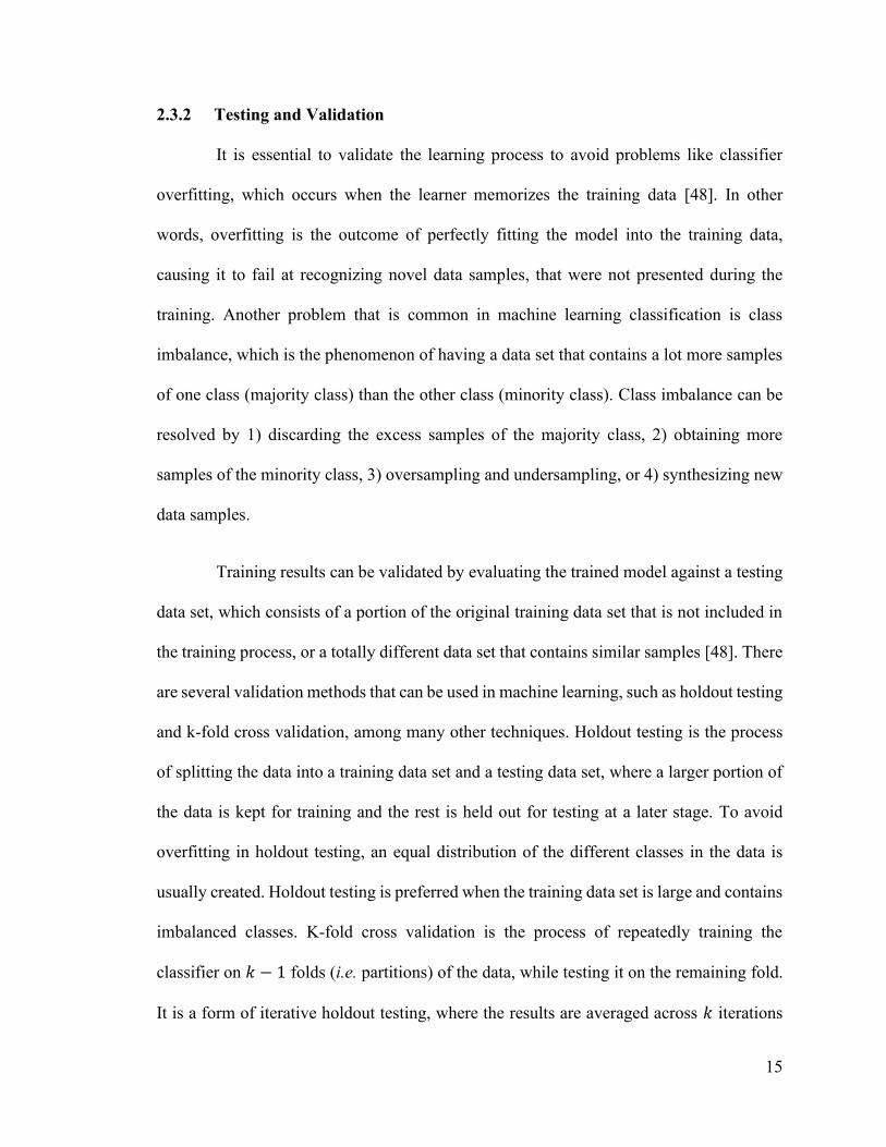
2.3.2 Testing and Validation
It is essential to validate the learning process to avoid problems like classifier
overfitting, which occurs when the learner memorizes the training data [48]. In other
words, overfitting is the outcome of perfectly fitting the model into the training data,
causing it to fail at recognizing novel data samples, that were not presented during the
training. Another problem that is common in machine learning classification is class
imbalance, which is the phenomenon of having a data set that contains a lot more samples
of one class (majority class) than the other class (minority class). Class imbalance can be
resolved by 1) discarding the excess samples of the majority class, 2) obtaining more
samples of the minority class, 3) oversampling and undersampling, or 4) synthesizing new
data samples.
Training results can be validated by evaluating the trained model against a testing
data set, which consists of a portion of the original training data set that is not included in
the training process, or a totally different data set that contains similar samples [48]. There
are several validation methods that can be used in machine learning, such as holdout testing
and k-fold cross validation, among many other techniques. Holdout testing is the process
of splitting the data into a training data set and a testing data set, where a larger portion of
the data is kept for training and the rest is held out for testing at a later stage. To avoid
overfitting in holdout testing, an equal distribution of the different classes in the data is
usually created. Holdout testing is preferred when the training data set is large and contains
imbalanced classes. K-fold cross validation is the process of repeatedly training the
classifier on 𝑘 − 1 folds (i.e. partitions) of the data, while testing it on the remaining fold.
It is a form of iterative holdout testing, where the results are averaged across 𝑘 iterations

16
to determine the final decision. This is good to continually evaluate the capability of the
classifier to recognize new, unseen data, and thus, helps to avoid overfitting. In this work,
5-fold cross validation was used to protect the classifiers against overfitting.
2.3.3 Performance Metrics
The performance of a classifier can then be measured by comparing the predicted
classes with the true classes of the data samples [48]. There are different metrics that can
be calculated to measure the performance of a classifier: accuracy, precision, sensitivity,
specificity, and F-score. In the case of binary classification, such metrics can be determined
using the number of true positives (TP), true negatives (TN), false positives (FP), and false
negatives (FN).
True positives are the samples that are classified positive and actually belong to
the positive class, while true negatives are the samples that are classified negative and
actually belong to the negative class [48]. False positives are the samples that are classified
positive but belong to the negative class, while false negatives are the samples that are
classified negative but belong to the positive class. Accuracy is the measure of correctly
classified samples (i.e. rate of true samples among all samples), that is:
𝐴𝑐𝑐𝑢𝑟𝑎𝑐𝑦 =𝑇𝑃 + 𝑇𝑁
𝑁 (1)
where N is the total number of samples. Precision measures the correctness in positive
predictions (i.e. rate of TP among all positive predictions), that is:
𝑃𝑟𝑒𝑐𝑖𝑠𝑖𝑜𝑛 =𝑇𝑃
𝑇𝑃 + 𝐹𝑃 (2)

17
Sensitivity is the measure of correctly classified positives (i.e. true positive rate), whereas
specificity is the measure of correctly classified negatives (i.e. true negative rate), that is:
𝑆𝑒𝑛𝑠𝑖𝑡𝑖𝑣𝑖𝑡𝑦 =𝑇𝑃
𝑇𝑃 + 𝐹𝑁 (3)
𝑆𝑝𝑒𝑐𝑖𝑓𝑖𝑐𝑖𝑡𝑦 =𝑇𝑁
𝑇𝑁 + 𝐹𝑃 (4)
The F-score (F1) is the harmonic mean of precision and sensitivity, which can be calculated
as follows:
𝐹1 = 2 ∙𝑝𝑟𝑒𝑐𝑖𝑠𝑖𝑜𝑛 ∙ 𝑠𝑒𝑛𝑠𝑖𝑡𝑖𝑣𝑖𝑡𝑦
𝑝𝑟𝑒𝑐𝑖𝑠𝑖𝑜𝑛 + 𝑠𝑒𝑛𝑠𝑖𝑡𝑖𝑣𝑖𝑡𝑦
=2𝑇𝑃
2𝑇𝑃 + 𝐹𝑃 + 𝐹𝑁
(5)
A confusion matrix is usually used to summarize TP, TN, FP, and FN. The rows of a
confusion matrix represent the true class (e.g. activity) of the data samples, whereas the
columns represent the class that the learner predicted, accordingly.
In multiclass classification problems, one can use true and false ratios for each
class instead of limiting the ratios to TP, TN, FP, and FN, for a total of 𝑛 × 2 ratios, where
𝑛 represents the number of classes. The performance metrics can then be calculated using
the true and false ratios of all classes.
2.4 Deep Learning
Deep learning is an advanced type of machine learning. Deep learners are neural
networks that are deep and have many neurons [50]. Deep learning models are usually

18
composed of multiple levels of abstraction, where the backpropagation algorithm is used
to determine the amount of adjustment in a machine’s parameters from one level to the
next. They have the potential to analyze patterns associated with complex forms of data.
Deep learning models can be trained on data sets of images, videos, sequences, or time
series. Hence, they enable complex applications, such as speech recognition, face
recognition, and activity recognition.

19
Chapter 3: Equipment
This chapter describes the equipment used to accomplish the contributions proposed
in this thesis.
3.1 Theory of Operation of the Equipment
This work was developed in collaboration with industry. Aerial Technologies
supported the work by providing their platforms for motion detection to determine if they
could also accomplish human activity recognition. Aerial’s motion detection technology
leverages the patterns in Wi-Fi signals propagating between two connected Wi-Fi devices
(transmitter and receiver) to analyze and detect the intensity of motion within an area of
coverage [51]. The detection then occurs in the range of an ellipsoid around the two
connected Wi-Fi devices, acting as the focal points. The highest motion intensities are
detected when moving near the devices or in the direct path between the two devices.
Although the intensity of motion reduces at other positions, motion would still be detected
as long as movements are happening in the coverage area (i.e. ellipsoid shape in Figure 1).
Figure 1 illustrates an example of a detection area.
Figure 1 Detection Area [51]

20
The size and shape of the detection area can be altered by many factors, such as the
shape, size and layout of the place; furniture and obstacles; building materials; as well as
the distance between the Aerial devices [51]. The detection area increases and decreases
with the distance between the devices. The two Wi-Fi devices consist of an AP and a client
station (STA) in Figure 1, each having a different functionality. These devices are designed
and tested in a laboratory environment, and they have no shielding. Hence, they are affected
by electromagnetic interference when placed within a small proximity of other wireless
devices and/or machines, such as computers.
The maximum detection area that can be covered by the Aerial devices is
approximately 1,200 square feet (110 square meters) [51]. A single AP-STA pair might not
be enough to guarantee complete coverage of larger spaces, in which case, multiple AP-
STA pairs may be used. Also, it is highly recommended to place the devices in the most
visited areas such as entrances, hallways, living rooms, etc. for better coverage, with fewer
devices.
3.2 Working Principle of the Equipment
Aerial Technologies provides an AP and a STA that can collect CSI data according
to the IEEE 802.11n and IEEE 802.11ac standards [51]. The AP acts as the transmitter,
whereas the STA acts as the receiver. Each device contains four antennas, which results in
16 potential active streams. Figure 2 shows the manner in which the Wi-Fi signal is
propagated from the transmitter to the receiver, having a direct path and multipath
components due to reflections and diffractions on objects and walls. Each spatial stream
contains multiple subcarriers in the frequency domain. The sampling rate of the system is
pre-set to 20 packets or samples per second, while the bandwidth is pre-set to 80 megahertz.

21
Figure 2 Signal Propagation © 2019 [1]
The obtained CSI packets from all links and subcarriers are indexed over time [33]
© 2019 [1]. Let 𝑙 ∈ {1, ⋯ , 𝐿} represent the antenna link, and 𝐶𝑆𝐼𝑖𝑙(𝑡) represent a complex
number, describing the signal received at subcarrier 𝑖 ∈ {1, ⋯ , 𝐼} at time 𝑡, defined by [33]:
𝐶𝑆𝐼𝑖𝑙(𝑡) = |𝐶𝑆𝐼𝑖𝑙(𝑡)| 𝑒∠𝐶𝑆𝐼𝑖𝑙(𝑡) (6)
For a total of 16 streams with 58 subcarriers each, data samples consist of CSI
measurements in the form of 3D matrices © 2019 [1]:
𝑠𝑢𝑏𝑐𝑎𝑟𝑟𝑖𝑒𝑟 𝑖𝑛𝑑𝑖𝑐𝑒𝑠 × 𝑝𝑎𝑐𝑘𝑒𝑡𝑠 × 𝑠𝑡𝑟𝑒𝑎𝑚𝑠 (7)
3.3 Deployment of the Equipment
The Aerial system was deployed in a 19 × 35 feet laboratory. The Wi-Fi devices
(AP and STA) were placed diagonally across the laboratory. Initially, the two devices were
both placed on the ground, at the corners of the laboratory, to perform 2D CSI
measurements. Any captures collected under this setting are missing elevation information.
Therefore, the AP was later mounted on the ceiling to perform 3D CSI measurements.
The Local Access Network (LAN) port of the provided AP device was connected to
a port on the laboratory’s router using an Ethernet cable. The AP device must always be
plugged in and connected to the Internet, as it is responsible for reporting CSI captures to

22
Aerial’s cloud engine. On the other hand, the STA device just needs to be connected to a
power outlet.
Aerial’s Android application can be used to record data samples, and for live (real-
time) demonstrations. An Application Programming Interface (API) is called by the
application every 2 seconds to store data in Aerial’s cloud. Aerial’s app was installed on
an Acer tablet, which was connected to the same network as the AP and STA. The app was
configured by 1) pairing it to the AP device, and 2) signing up and creating a profile to
associate with the AP device. Figure 3 below displays the deployment topology and the
involved components. This system was used to acquire data for the thesis.
Figure 3 Deployment Topology and Components

23
Chapter 4: Proposed Solution
Aerial’s system was utilized to distinguish between two similar motions: the actions
of sitting-down and standing-up from each other, and from the still (seated or standstill)
case. The solution is composed of five main blocks: data collection and conversion, data
preprocessing, feature extraction and scaling, class balancing, and classification. The data
collection block is the stage at which sitting and standing experiments were performed to
acquire the required Wi-Fi CSI signals for the study. The data preprocessing block is
necessary to put the data in a proper format. Feature extraction is essential to determine
attributes that identify an activity, as well as to reduce the dimensionality of the data. The
class balancing block ensures that there is an equal distribution of data samples across all
activity classes. Lastly, the classification block is split into two stages: training and testing.
Sections 4.1 through 4.5 will discuss these five blocks, respectively. Figure 4 provides an
overview of the developed system.
Figure 4 System Overview
This chapter covers contributions 1 and 2. Contribution 1 focuses on performing data
collection, preprocessing, visualization, and analysis on CSI captures; while contribution
2 focuses on applying a supervised machine learning technique to distinguish among
sitting-down and standing-up actions. The following sections describe the proposed
solution in more details.
24
4.1 Data Collection
The first block in the system is data collection (see Figure 4). Test scenarios of
differing sitting and standing speeds and styles, within various room arrangements, were
conducted using the setup detailed in section 3.3 to address as many variations as could be
tested © 2019 [1]. Various experimental setups were explored in terms of the position of
Wi-Fi devices (AP and SAT/transmitter and receiver), and the location of activities relative
to the devices. CSI data for a sequence of sitting-down and standing-up activities were
acquired, as performed by a single subject, multiple times. Thus, four data sets were
generated to represent data collected for:
1. a single activity location with both devices (i.e. AP and STA) on ground, as
shown in Figure 11;
2. multiple activity locations, as shown in Figure 12, with both devices on
ground;
3. multiple activity locations, as shown in Figure 12, with the AP at the ceiling
and the STA on the ground; and
4. all cases combined (data sets 1, 2 and 3).
Also, three volunteers were later asked to perform similar sitting and standing activities, at
random room locations, with the AP mounted at the ceiling and the STA on the ground.
Appendix A contains table summaries of the data collected and used for experimentation
in this thesis.
The collected data consisted of 3D CSI captures, where each reading was a complex
number of the form |𝐶𝑆𝐼𝑖𝑙(𝑡)| 𝑒∠𝐶𝑆𝐼𝑖𝑙(𝑡). Each CSI reading is collected by a specific

25
subcarrier, at a specific timestamp. Each timestamp roughly corresponds to a second in
time. With a sampling rate of 20 packets per second, about 1,800 packets of data were
captured per sample, by 58 subcarriers, at 16 different streams. As such, the data consisted
of 58 × 16 time series of CSI measurements. Figure 5 shows a sample of the magnitudes
of a raw CSI capture, for one stream.
Figure 5 Raw CSI Capture
4.2 Data Preprocessing
The second block in the system is data preprocessing (see Figure 4). The acquired
data/signals were preprocessed with filtering, dimensionality reduction, and segmentation
© 2019 [1]. The signals were segmented and labelled as still, sitting-down, or standing-up.
Then, a set of features was then extracted and scaled between 0 and 1 (see section 4.3). It
was important to balance the classes in the data to improve the classification process (see
section 4.4). Lastly, a series of traditional machine learning classifiers was used to
distinguish among three classes of motion: stationary (seated or standing still), sitting-
down, and standing-up (see section 4.5). The remainder of this section will further discuss
the data preprocessing methodology.

26
Since all streams reflect the same signal, one stream, rather than on all 16, was chosen
to operate on © 2019 [1]. As such, the best spatial stream (i.e. the one with the highest
signal power and the lowest mean variance) was selected based on RSS and stability. The
highest power represented the strongest signal, while the lowest long-term variance
constituted a consistent, stable signal. This approach enabled us to operate on the stream
that was mostly affected by the human activity.
The raw CSI measurements (complex numbers) in the selected stream were divided
into their amplitudes, phases, and magnitudes (i.e. the square root of the sum of squared
amplitude and phase components) © 2019 [1]. Then, a Hampel filter was applied to
eliminate any outliers as suggested by [37], [38], and [45], along with a low-pass filter for
noise removal. Since no human activity exceeds 2 hertz [33], the cut-off frequency of the
low-pass filter was set to 2 hertz. Figure 6 displays a sample CSI capture after filtering.
Figure 6 Filtered CSI Capture
Lastly, the CSI signals were segmented into 20-packet windows and accordingly
labelled © 2019 [1]. A window length of 20 was chosen because some sitting-down and

27
standing-up activities only take 1 second (i.e. about 20 packets) to complete. A timestamp
was attached to each packet. To segment and label the data, the timestamps attached to the
packets, as well as the event times recorded while performing sequences of sitting-down
and standing-up activities, were utilized. This was achieved by finding the minimum
absolute difference between an event’s timestamp and the timestamps of the packets. Each
event timestamp marked the beginning or the end of a stationary, sitting-down, or standing-
up activity. Once the appropriate starting timestamp/packet for an activity was located, the
signal was segmented into 20-packet segments until the next event’s timestamp was
reached.
4.3 Feature Extraction and Selection
The third block in the system is feature extraction and scaling (see Figure 4). To
reduce the dimensionality of the problem, the data was transformed from 3D to 2D by
calculating metrics such as kurtosis, maximum, mean, minimum, skew, standard deviation,
and variance along the subcarrier domain © 2019 [1]. The calculated attributes were chosen
as they are commonly used across multiple state-of-the-art studies [32 - 47]. After this step,
each data sample was represented as a time series of measured attributes. Figure 7 shows
a sample plot of these time series in terms of features calculated on the magnitude of CSI
measurements. One can observe that the time series seem to have some sort of a pattern
associated with the movement from a sitting to a standing position, and vice versa (arrows
in Figure 7). This pattern was evident on all of the attributes, which justified their selection
for further analysis. Nonetheless, the moving variance of the mean as well as the moving
variance of the variance, over a sliding window of 20 packets, were explored to more

28
clearly visualize the patterns associated with the movements from a sitting to a standing
position, and vice versa © 2019 [1].
Figure 7 Sample Time Series of Subcarrier Features © 2019 [1]
Figure 8 Sample Plots for Moving Variance of the Mean and of the Variance © 2019 [1]
Figure 8 represents a sample plot of the moving variance of the mean and the moving
variance of the variance. Each peak is associated with a sitting-down or a standing-up

29
activity, which shows a great potential to recognize human activities from the CSI of Wi-
Fi signals. Therefore, these peaks were used as another feature.
To deal with time series, the dimensionality of the data was further reduced by
calculating metrics over the time (packet) domain © 2019 [1]. As a result, the final feature
space, illustrated in Figure 9, was constructed at three levels:
1. Complex features, which consisted of 3D arrays of the amplitudes, phases,
and magnitudes of raw CSI measurements (third dimension), obtained over
time and sampled as packets (second dimension), by 58 subcarriers (first
dimension), in the best spatial stream;
2. Subcarrier features, which consisted of 2D arrays of the kurtoses, maximums,
means, minimums, skews, standard deviations, and variances of complex
features (second dimension), calculated over the subcarrier domain (reduced
dimension), for each packet (first dimension); and
3. Time features, which consisted of 1D points of the kurtosis, maximum, mean,
minimum, peak, skew, standard deviation, and variance of subcarrier
features, calculated across packets (reduced dimension).
As such, the feature space contained a total of 168 features per data sample. The 3D
complex features were represented as three different matrices: CSI amplitudes, phases, and
magnitudes, in terms of both subcarrier indices and packets of time. To reduce the
subcarriers dimension, the 2D subcarrier features were calculated as 21 time series of
kurtoses, maximums, means, minimums, skewnesses, standard deviations, and variances,
for each of the 3D matrices in the set of complex features (i.e. CSI amplitudes, phases, and

30
magnitudes). Finally, to reduce the packets dimension, the time features were determined
for each packet, by calculating the kurtosis, maximum, mean, minimum, peak of moving
variance of the mean, peak of moving variance of the variance, skewness, standard
deviation, and variance of each of the 2D time series in the set of subcarrier features.
Figure 9 The Three Levels of Extracted Features
To bring all values into the range [0 1], feature scaling was applied on these features
via the following formula © 2019 [1]:
𝑥𝑖′ =
𝑥𝑖 − 𝑋𝑚𝑖𝑛
𝑋𝑚𝑎𝑥 − 𝑋𝑚𝑖𝑛 (8)
where 𝑋𝑚𝑖𝑛 and 𝑋𝑚𝑎𝑥 are the minimum and maximum values of a feature vector. This
approach is also known as min-max normalization. The range of all features should be
normalized for them to contribute proportionately to the final decision of the classifiers.

31
Feature scaling was tested by scaling the features space 1) over the subcarrier domain by
normalizing the 2D subcarrier features, 2) across the time domain by normalizing the 1D
time features, and 3) both ways (1 and 2). The third option improved the classification
performance the most, as demonstrated using experimental results in section 5.2.3.
4.4 Class Imbalance
The fourth block in the system is class balancing (see Figure 4). Since the main
interest was in the dynamics of the movements, lifting off the chair was counted as a
“standing-up” activity, whereas getting on the chair was considered to be a “sitting-down”
activity © 2019 [1]. To label the data, three labels (i.e. classes) were used: still (seated or
standstill), sitting-down, and standing-up. Due to the nature of the employed data
collection, the collected data contained more samples belonging to the “still” class, and, as
such, the data set was imbalanced. To tackle this issue, the ADAptive SYNthetic Sampling
(ADASYN) technique [52] was utilized to reduce class imbalance by synthesizing new
samples of the minority class around the boundary between two classes instead of the
interior of the minority class. This technique is an extension of the Synthetic Minority
Oversampling TEchnique (SMOTE), which synthesizes new samples through a linear
interpolation between existing minority class samples. In the context of this work,
ADASYN was first applied to generate more samples of the “sitting-down” class as
opposed to the “still” class. Then, it was applied to generate more samples of the “standing-
up” class as opposed to the “still” class. Afterwards, the synthesized “sitting-down” and
“standing-up” samples were combined with the original data set. The used implementation
of the ADASYN method takes six input parameters: a matrix of features, a vector of labels,
the desired level of balance, the density of neighbors (for the k-nearest neighbors – KNN

32
– call used in ADASYN [52]), the density for the KNN call used in SMOTE, and a Boolean
that specifies if the features are normalized. The density parameters were set to 5 by default,
while the normalization parameter was set to false. Setting the normalization parameter to
false triggers unit variance normalization. The ADASYN method did not only assist in
solving the class imbalance issue, but also provided more data to train the classifiers on.
4.5 Classification
The fifth block in the system is classification (see Figure 4). In terms of classification,
both classical classifiers and deep learning classifiers were attempted. MATLAB’s
Classification Learner and Deep Network Designer apps were used to test a number of
classification models. The following sections will discuss the classification methodologies
in further details.
4.5.1 Classification via Traditional Machine Learning
MATLAB’s Classification Learner was used to train different classifiers on the
collected data © 2019 [1]. All available classifiers were leveraged to compare their
classification performances, with 5-fold cross validation, to prevent them from overfitting.
The tested classifiers included decision trees, discriminant analysis, naïve Bayes, SVMs,
KNN, and ensemble classifiers. The “No Free Lunch” theorem applies here, in the sense
that there is no one classifier that works best in all circumstances. The performance of the
classifiers is very dependent on the available data. However, the literature has shown use
of decision tree [19, 20, 32], naïve Bayes [9, 20], SVM [9, 15, 20, 45, 46], and KNN [20]
classifiers among others that were not utilized by the author of this thesis.
33
For the decision trees, the fine, medium, and coarse versions were used. A fine
decision tree has many leaves, and makes many fine distinctions between classes with a
maximum number of 100 splits. A medium decision tree is a medium-complexity decision
tree that has fewer leaves, and a maximum number of 20 splits, while a coarse decision tree
has few leaves, and makes coarse distinctions between classes with a maximum number of
4 splits.
In terms of discriminant analysis, linear and quadratic discriminant classifiers with
diagonal covariance regularization were tested. A linear discriminant is, in general, a faster
and easier-to-interpret classifier, which creates linear boundaries between classes, while a
quadratic discriminant classifier creates more complex (elliptical, parabolic, or hyperbolic)
boundaries between classes, and, as such, has the potential to improve the classification.
To keep up with recent advances in research such as [9] and [20], naïve Bayes
classifiers were added to the analysis © 2019 [1]. More specifically, two naïve Bayes
approaches were tested: Gaussian and kernel. A Gaussian naïve Bayes classifier uses a
Gaussian distribution for numeric predictors, while a kernel naïve Bayes classifier uses a
kernel distribution, with a Gaussian kernel type and unbounded support. Both Gaussian
and kernel naïve Bayes classifiers use a MultiVariate MultiNomial (MVMN) distribution
for categorical predictors.
Among the SVMs, linear, quadratic, cubic, fine Gaussian, medium Gaussian, and
coarse Gaussian SVMs were tested © 2019 [1]. The linear, quadratic, and cubic SVMs
differ, as in the case of the discriminants above, in the complexity of the boundary that they
create between classes. The fine, medium, and coarse Gaussian SVMs all use Gaussian
kernels that differ in size. A fine Gaussian SVM enables finely-detailed distinctions

34
between classes, using a Gaussian kernel with the kernel scale set to 𝑠𝑞𝑟𝑡(𝑃)/4, where 𝑃
is the number of predictors (i.e. features). A medium Gaussian SVM makes fewer
distinctions between classes, using the Gaussian kernel with the kernel scale set to 𝑠𝑞𝑟𝑡(𝑃).
Finally, a coarse Gaussian SVM makes coarse distinctions between classes, using the
Gaussian kernel with the kernel scale set to 𝑠𝑞𝑟𝑡(𝑃) ∗ 4.
For the KNN classifiers, the fine, medium, coarse, cosine, cubic, and weighted
versions were tested © 2019 [1]. The fine, medium, and coarse KNN classifiers make
distinctions between classes using a Euclidean distance metric and equal distance weight,
with the number of neighbours set to 1, 10, and 100, respectively. A cosine KNN classifier
uses the cosine distance metric and equal distance weight, with the number of neighbours
set to 10, while a cubic KNN classifier uses the cubic distance metric, Minkowski, and
equal distance weight, with the number of neighbours set to 10. A weighted KNN classifier
uses a Euclidean distance metric and squared inverse distance weight, with the number of
neighbours set to 10.
Decision trees are constructed from conditional statements based on the boundaries
in the variables of the inputted training data set, where each branch represents a condition
and outputs a decision [48]. Discriminant analysis is the process of distinguishing between
two or more classes using a boundary function. Naïve Bayes classification depends on a
collection of probabilistic algorithms that are based on Bayes’ theorem, which views each
feature independently. SVMs attempt to identify the optimal hyperplane for categorizing
data samples. An optimal hyperplane defines a clear gap between the data points in terms
of space. The KNN algorithm determines the class of a sample according to its 𝑘 nearest
neighbours.

35
Finally, five different ensemble classifiers were also tried: boosted trees, bagged
trees, subspace discriminant, subspace KNN, and RUSBoosted trees © 2019 [1]. The
boosted trees model creates an ensemble of 30 medium decision trees using the AdaBoost
algorithm. It uses relatively little memory or time, but might require more ensemble
members than bagged trees. The bagged trees model is a bootstrap-aggregated ensemble
of 30 fine decision trees. This type of model is often very accurate, but can be slow and
memory-intensive for large data sets. The subspace models use the random subspace
algorithm to create an ensemble of classifiers, with a subspace dimension of 𝑃/2. The
subspace discriminant model creates an ensemble of 30 discriminant classifiers, whereas
the subspace KNN model creates an ensemble of 30 KNN classifiers. They are good for
many predictors (i.e. features), relatively fast for fitting and prediction, and low on memory
usage. However, their performance can vary depending on the data. The RUSBoosted trees
model is an extension of the boosted trees model. It is usually used when there is a skew in
the data, with many more observations of one class (i.e. class imbalance (see section 4.4)).
The next section will cover the proposed deep learning methodology.
4.5.2 Classification via Deep Learning
MATLAB’s Deep Network Designer was used to design and implement a deep
learning model. A Bidirectional Long Short-Term Memory (BiLSTM) neural network was
designed to perform deep learning on the collected data. A BiLSTM network is a recurrent
neural network, dedicated for learning long-term dependencies among the time steps of
sequence data, and thus, is a good candidate for classifying the activities in the data set(s)
of this work. Figure 10 displays the layers of the designed network. The network starts with

36
a Sequence Input layer, and ends with a Fully Connected layer, a SoftMax layer, and a
Classification Output layer to facilitate the prediction of class labels.
Figure 10 Layers of Designed Neural Network
The Sequence Input layer allows for the sequence of 21 features to be inputted to
the network. Then, a BiLSTM layer of 128 hidden units/nodes, in default, is added to learn
the bidirectional long-term dependencies between the time steps of the inputted time series
(i.e. sequence data). These dependencies are useful for the network to learn from the
complete time series at each time step. The number of hidden units/nodes specifies the
amount of information that will be remembered between time steps. The Fully Connected
layer multiplies the input by a weight matrix and then adds a bias vector, with an output
size of 3 or 4 (number of activity classes). The SoftMax layer applies a softmax activation
function to the input to determine the probabilities distribution of each activity class over
all classes. Finally, the Classification Output layer computes the cross-entropy loss for

37
multi-class classification with mutually exclusive classes. The cross-entropy loss is a
measurement of performance.
Signals, such as the one shown in Figure 7, have been used to perform deep
learning using the designed BiLSTM network. These signals represent the subcarrier
features, which are time series of seven attributes: mean, minimum, maximum, variance,
standard deviation, kurtosis, and skewness; calculated over the subcarrier domain of 3D
matrices of CSI amplitudes, phases, and magnitudes. As such, the resulting feature space
consists of 21 variables.
The ADAM (adaptive moment estimation) optimizer was then used to train the
designed network. The network was set to train for a maximum of 100 epochs, where an
epoch represents a full pass through the entire data set. Furthermore, the minimum batch
size was set to 20, meaning that the network is trained on 20 observations at each iteration
of an epoch. The validation frequency was set to 50 iterations.

38
Chapter 5: Experimental Results
This chapter will discuss the achieved experimental results for the contributions of
this thesis.
5.1 Distinguishing Sitting-down and Standing-up Activities
A “preliminary” data set was initially collected to perform basic test cases for the
proof of concept. This section includes details about the conducted experiments to collect
the so-called “preliminary” data set, and results showing that the solution proposed in
Chapter 4 can, in fact, distinguish between the dynamic motions of sitting-down and
standing-up activities.
5.1.1 Preliminary Sitting and Standing Experiments by One Subject
Initially, data about Wi-Fi’s CSI were collected by having one person (the author;
a healthy female, 25 years old, 160 centimeters high, and 57 kilograms in weight) perform
a sequence of sitting-down and standing-up activities at a single location in the room ©
2019 [1]. The system was tested on a set of sitting-down and standing-up activities for a
period of 90 seconds, as follows:
• sit for 5 seconds,
• stand for 15 seconds,
• sit for 15 seconds,
• stand for 15 seconds, and
• sit for the remaining time.

39
The subject also carried a timer to record her event times as she sat down and stood
up © 2019 [1]. This was done to keep track of the duration, as well as the start and end
times of activities to help with data segmentation and labelling later on. At the start of a
sequence of sitting-down and standing-up activities, the subject hit the timer’s start button.
Then, she waited for 5 seconds, hit the lap button, and started standing up. When she
finished standing up, she hit the lap button again. She waited 15 seconds in a standstill
position, hit the lap button, and started sitting down. Once fully seated, she hit the lap
button again, and so on, until she completed the sequence. The lap times were recorded as
a sequence of nine event times in minutes, seconds, and milliseconds, which corresponded
to the duration of the laps (i.e. roughly between 1 to 15 seconds each). The actual timestamp
of each event, within a sequence, was calculated by adding the preceding event times to its
time. Event timestamps were then used to segment the data into separate samples, for each
activity, as explained in section 4.2 above. Additionally, the activities were also video-
recorded to get a ground truth of the subject’s actions.
To allow the system to be able to identify a larger spectrum of sit-stand human
activities, the following variations of actions were proposed for the training data, which
was collected by the initial subject © 2019 [1]:
• sitting down and standing up in one step (i.e. no bending or leaning),
• sitting down and standing up in two steps by slightly bending forward then
standing up or sitting down, and
• sitting down and standing up in three steps by leaning, bending, then standing
up or sitting down.

40
This was repeated multiple times, while facing a different direction (forward, backward,
right, left, facing the transmitter/AP, facing the receiver/STA) each time © 2019 [1]. All
of these experiments were completed with a chair placed in the middle of the laboratory,
as in Figure 11.
Thus, a data set of CSI captures with the chair at the middle of the room, and both
devices placed at ground-level (the so-called “preliminary” data set), was obtained. It was
then filtered using both Hampel and low-pass filters, and segmented into 20-packet (1
second) segments. The so-called “preliminary” data set contained 2,835 samples. The
number of samples within the so-called “preliminary” data set was then increased to 7,576
by generating new samples to balance the classes (see section 4.4). The so-called
“preliminary” data set was used as a proof of concept data set to perform various tests.
5.1.2 Preliminary Results
The results for the preliminary case with the activity executed, by one individual,
in the middle of the laboratory and both devices on the floor (as illustrated in Figure 11)
are shown in Table 2, which summarizes the achieved classification accuracies. Note that
the data used here was only filtered via both a Hampel and a low-pass filter, without
applying any normalization or feature scaling yet.
Figure 11 Initial activity location with the chair placed in the middle of the room © 2019 [1]

41
Table 2 Preliminary Classification Results
Classification Method Type Accuracy (%)
Decision Trees (DTs)
Fine 77.9
Medium 68.0
Coarse 60.3
Discriminant Analysis (DA) Linear 57.1
Quadratic 53.2
Support Vector Machines (SVMs)
Linear 74.0
Quadratic 96.1
Cubic 97.2
Fine Gaussian 95.5
Medium Gaussian 97.5
Coarse Gaussian 70.5
K-Nearest Neighbours (KNN)
Fine 85.7
Medium 78.3
Coarse 60.2
Cosine 85.9
Cubic 77.0
Weighted 78.0
Ensemble Classifiers
Boosted Trees 76.2
Bagged Trees 96.1
Subspace Discriminant 73.7
Subspace KNN 75.0
RUSBoosted Trees 68.0
In this case, the maximum accuracy, achieved by the medium Gaussian SVM, was
97.5%. Accuracy is often not considered as a good estimate of classification performance,
since it only measures the ratio of correct predictions, regardless of the amount of incorrect
predictions. Therefore, confusion matrices will also be presented to offer a more complete
view of the classification performance.
Table 3 illustrates the confusion matrix of the predictions of the medium Gaussian
SVM for the so-called “preliminary” data set. As observed in the table, most samples were

42
classified correctly. The green cells represent the number of correctly classified samples,
while the pink cells represent the number of incorrectly classified samples. From 2,526
samples for the “still” class, 2,338 were correctly classified as still and 188 were wrongly
classified as sitting-down or standing-up. For the “sitting-down” class, from 2,526 samples,
2,525 were correctly classified as sitting-down and one was wrongly classified as still. For
the “standing-up” class, from 2,524 samples, 2,520 were correctly classified as standing-
up and 4 were wrongly classified.
Table 3 Confusion Matrix of the Medium Gaussian SVM for the “preliminary” Data Set
Tru
e C
lass
Still 2338 85 103
Sitting-down 1 2525 0
Standing-up 3 1 2520
Still Sitting-down Standing-up
Predicted Class
These results demonstrate that it is possible to use Wi-Fi CSI to distinguish
between the two similar motions of sitting-down and standing-up. Most of the utilized
classifiers achieved high accuracies, and only 193 samples (out of 7,576) were
misclassified by the best classifier.
5.2 Pre-processing Techniques
Based on the results in the previous section, additional preprocessing methods that
could potentially improve the classification performance of the system were studied. As
such, this section compares a number of preprocessing approaches to conclude regarding
the best approach in terms of classification performance, which constitutes the third
contribution of the thesis, from the list in section 1.4.

43
5.2.1 Experiments with Data Preprocessing Techniques
To study the impact on the classification performance, multiple data preprocessing
techniques were investigated. In particular, various normalization approaches were
explored:
1. standardizing the raw CSI measurements over subcarriers for each
packet/timestamp separately (or vice versa), using the z-score method:
𝑥𝑖′ = 𝑧𝑖 =
𝑥𝑖 − 𝜇
𝜎 (9)
where 𝑥𝑖 is a sample CSI amplitude, phase, or magnitude; while 𝜇 and 𝜎 are
the mean and the standard deviation of a vector of CSI amplitudes, phases, or
magnitudes, respectively. This approach normalized the data to have a mean
of 0 and a standard deviation of 1.
2. normalizing the raw CSI measurements over subcarriers for each
packet/timestamp separately (or vice versa), using the following fixed-factor
formula, determined by Aerial:
𝑋′ = 𝑛𝑜𝑟𝑚𝑎𝑙𝑖𝑧𝑎𝑡𝑖𝑜𝑛 𝑓𝑎𝑐𝑡𝑜𝑟 ∙ 𝑋 (10)
𝑛𝑜𝑟𝑚𝑎𝑙𝑖𝑧𝑎𝑡𝑖𝑜𝑛 𝑓𝑎𝑐𝑡𝑜𝑟
= √(1𝑒6 ∗ 1.6508)(𝑋 ∙ 𝑋𝑇)
(11)
where 𝑋 is a vector of CSI amplitudes, phases, or magnitudes; and 𝑋𝑇 is the
transpose of 𝑋.

44
As can be seen in the following sections, the z-score standardization approach noticeably
enhanced the performance over the other approaches.
5.2.2 CSI Normalization
As mentioned in section 5.2.1 above, multiple data preprocessing techniques were
explored, beyond filtering. The explored techniques include normalizing the data using z-
score standardization, or by a normalization factor. The data were normalized over the time
domain and over the subcarrier domain. Normalizing the data over the subcarriers, using
z-score standardization, had a better effect on the classification performance. Table 4 below
compares the classification accuracies of the different classifiers, after applying the
aforementioned normalization methods, on the so-called “preliminary” data set.
As observed in the table, standardization via the z-score method, across the
subcarriers per timestamp significantly improved the classification performance over the
other approaches. It achieved a maximum accuracy of 98.5% by the medium Gaussian
SVM.
5.2.3 Feature Scaling
Feature scaling is essential to normalize the range of all features between 0 and 1,
for them to contribute proportionately to the prediction of the classifiers. Feature scaling
was performed on the 2D subcarrier features (i.e. time series), the 1D time features (i.e.
data points), and on both. Scaling the 2D subcarrier features as well as scaling all features,
at both the 2D level and again at the 1D level, produced similar classification accuracies,
as can be seen in Table 5. The first approach (scaling the 2D subcarrier features) achieved
a maximum accuracy of 98.5% by the medium Gaussian SVM.

45
Table 4 Comparison of Classification Accuracies achieved by Normalization Approaches
Classification
Method Type
Accuracy (%)
z-score
(time)
factor
(time)
z-score
(subcarriers)
factor
(subcarriers)
Decision Trees
(DTs)
Fine 77.1 77.3 75.7 76.7
Medium 68.4 69.5 66.8 66.8
Coarse 60.3 61.5 58.2 60.3
Discriminant
Analysis (DA)
Linear 55.8 52.1 55.5 58.3
Quadratic 58.3 58.0 33.9 56.9
Support Vector
Machines (SVMs)
Linear 76.0 74.4 76.7 73.0
Quadratic 96.2 95.8 96.5 95.9
Cubic 97.6 97.3 97.6 96.9
Fine
Gaussian 92.3 92.6 92.0 92.8
Medium
Gaussian 97.9 97.8 98.5 97.3
Coarse
Gaussian 74.0 71.6 73.7 71.6
K-Nearest
Neighbours (KNN)
Fine 85.5 84.7 81.7 85.4
Medium 77.9 76.4 73.4 77.6
Coarse 61.4 59.9 58.1 60.4
Cosine 87.9 85.1 83.5 86.1
Cubic 76.6 75.7 73.1 76.9
Weighted 77.8 76.5 73.2 77.4
Ensemble
Classifiers
Boosted
Trees 74.8 75.7 75.3 72.8
Bagged
Trees 96.2 96.8 95.8 95.8
Subspace
Discriminant 73.6 73.7 69.7 73.0
Subspace
KNN 92.0 64.8 88.4 87.4
RUSBoosted
Trees 69.4 70.1 69.0 67.4
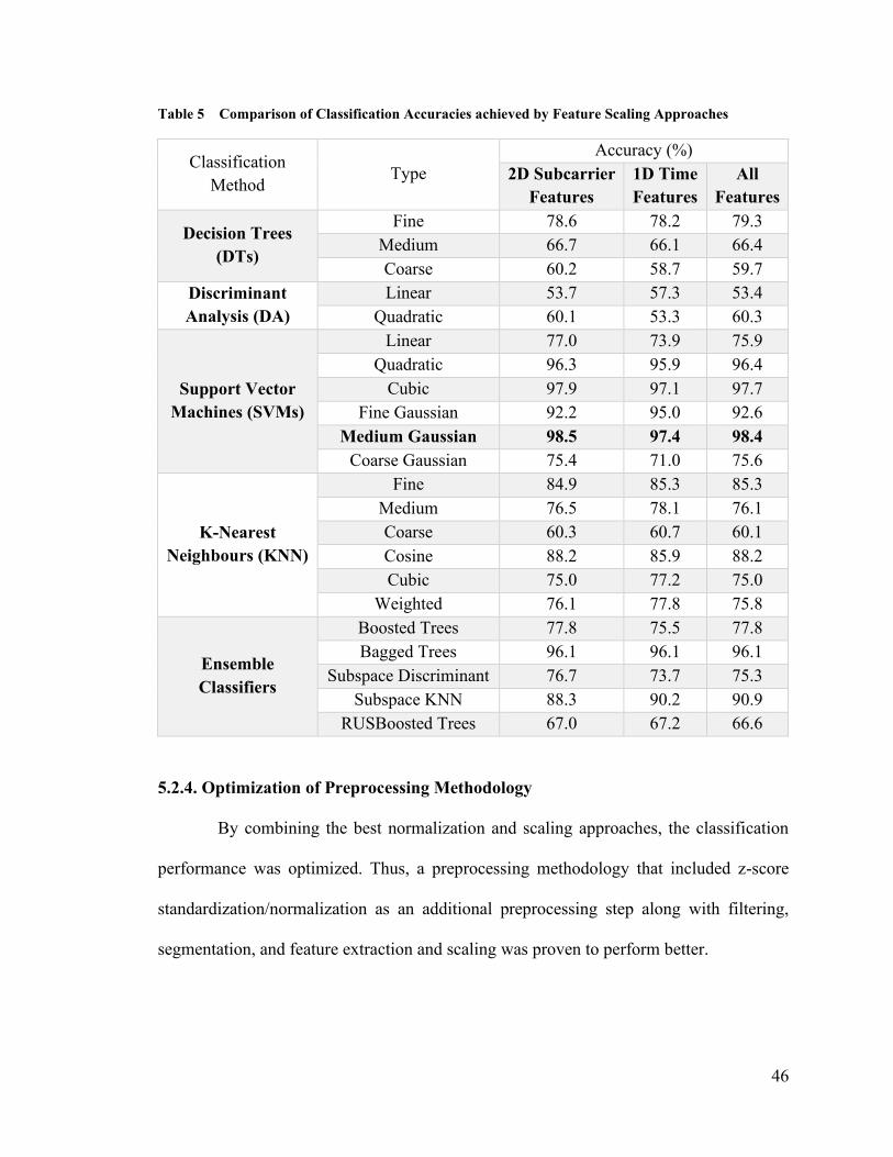
46
Table 5 Comparison of Classification Accuracies achieved by Feature Scaling Approaches
Classification
Method Type
Accuracy (%)
2D Subcarrier
Features
1D Time
Features
All
Features
Decision Trees
(DTs)
Fine 78.6 78.2 79.3
Medium 66.7 66.1 66.4
Coarse 60.2 58.7 59.7
Discriminant
Analysis (DA)
Linear 53.7 57.3 53.4
Quadratic 60.1 53.3 60.3
Support Vector
Machines (SVMs)
Linear 77.0 73.9 75.9
Quadratic 96.3 95.9 96.4
Cubic 97.9 97.1 97.7
Fine Gaussian 92.2 95.0 92.6
Medium Gaussian 98.5 97.4 98.4
Coarse Gaussian 75.4 71.0 75.6
K-Nearest
Neighbours (KNN)
Fine 84.9 85.3 85.3
Medium 76.5 78.1 76.1
Coarse 60.3 60.7 60.1
Cosine 88.2 85.9 88.2
Cubic 75.0 77.2 75.0
Weighted 76.1 77.8 75.8
Ensemble
Classifiers
Boosted Trees 77.8 75.5 77.8
Bagged Trees 96.1 96.1 96.1
Subspace Discriminant 76.7 73.7 75.3
Subspace KNN 88.3 90.2 90.9
RUSBoosted Trees 67.0 67.2 66.6
5.2.4. Optimization of Preprocessing Methodology
By combining the best normalization and scaling approaches, the classification
performance was optimized. Thus, a preprocessing methodology that included z-score
standardization/normalization as an additional preprocessing step along with filtering,
segmentation, and feature extraction and scaling was proven to perform better.

47
Table 6 summarizes the classification accuracies after 1) standardizing the CSI
data, over the subcarriers domain, through the z-score method, and 2) scaling subcarrier
features or all features.
Table 6 Classification Results with Optimum Preprocessing Methodology
Classification
Method Type
Accuracy (%)
Subcarrier Features All Features
Decision Trees
(DTs)
Fine 75.9 75.7
Medium 67.0 66.6
Coarse 58.3 58.8
Discriminant
Analysis (DA)
Linear 56.6 56.5
Quadratic 65.1 66.1
Support Vector
Machines (SVMs)
Linear 74.3 75.3
Quadratic 96.6 96.8
Cubic 97.7 97.8
Fine Gaussian 90.1 90.6
Medium Gaussian 98.8 98.8
Coarse Gaussian 74.7 74.7
K-Nearest
Neighbours
(KNN)
Fine 82.3 82.2
Medium 73.3 73.2
Coarse 58.3 57.2
Cosine 86.9 86.8
Cubic 72.2 72.2
Weighted 73.1 72.8
Ensemble
Classifiers
Boosted Trees 75.5 75.7
Bagged Trees 96.7 96.5
Subspace Discriminant 73.3 73.1
Subspace KNN 87.4 87.8
RUSBoosted Trees 69.2 68.7
By comparing Tables 2, 4, 5 and 6, one can observe that applying a preprocessing
methodology that includes both z-score standardization over the subcarriers and scaling all
features improved the performance for most classifiers. For example, the maximum
accuracy, achieved by the medium Gaussian SVM, went up to 98.8% for the so-called

48
“preliminary” data set. Therefore, the results presented in the following sections are all
presented for data that was preprocessed by filtering, z-score standardization, and by
scaling all features.
Appendix B presents samples of the signals produced by applying the different
preprocessing techniques.
5.3 Subject Activity and Device Location Independence
Once the first series of results demonstrated that the proposed solution distinguishes
between still, sitting-down, and standing-up activity classes, different activity and device
locations were also investigated. These are related to contributions 4 and 5 from the list in
section 1.4. Contribution 4 focuses on the validation of the proposed solution for location
and participant movement independence, while contribution 5 focuses on the impact of the
location of Wi-Fi sensor devices on the classification. This section explains these
contributions, by supporting them with additional experimental results.
5.3.1 Experiments on Activity Location Independence
As already briefly mentioned in section 4.1, the capability of the system to deal
with different variations was explored. First, the location of the chair was changed, while
keeping both the transmitter and the receiver on the ground. The chair was then positioned
near the transmitter, near the receiver, and at the two empty corners of the room. All of the
experiments were repeated with the transmitter mounted on the ceiling. Thus, test scenarios
of differing sitting and standing speeds and styles were conducted, by one individual,
within various room arrangements, to address as many variations as possible. Five
experimental setups in terms of the position of Wi-Fi devices, and the location of activities

49
relative to the devices were explored. Figure 12 shows top views of the various
experimental setups.
a) Initial activity location with the chair placed in the middle of the room
b) Second activity location with the chair placed
near the transmitter
c) Third activity location with the chair placed near
the receiver
d) Fourth activity location with the chair placed at
the front-left corner
e) Fifth activity location with the chair placed at
the back-righ corner
Figure 12 Top Views of Experimental Setups
In a real-life situation, a chair could be placed anywhere in a room. By changing
the position of the chair around the laboratory, relative to the Wi-Fi devices, the system
was enabled to identify more cases of sitting-down and standing-up activities. In turn, a
data set was acquired for all scenarios and activity locations, with both devices placed at
ground-level (the “floor” data set). Mounting one of the Wi-Fi devices at the ceiling of the

50
laboratory added a third dimension to the CSI measurements. This helped to account for
elevation information, such as the height of a person, in the sensed motions. Also, this
enabled the sensing of Wi-Fi signals’ propagation throughout the whole room, rather than
propagating at the level of the ground only. Hence, this provided more coverage of the
room in terms of both connectivity, and motion detection and identification. As a result, a
data set of all scenarios and activity locations was acquired, with one device placed at
ground-level and the other mounted at the ceiling (the “ceiling” data set). The so-called
“preliminary”, “floor”, and “ceiling” data sets were then combined into one data set: the
“floor + ceiling” data set. To summarize, four different data sets were acquired:
1. a preliminary data set with the chair at the middle of the room and both
devices placed at ground-level (preliminary);
2. a data set of all scenarios and activity locations with both devices placed at
ground-level (floor);
3. a data set of all scenarios and activity locations with one device placed at
ground-level and the other mounted at the ceiling (ceiling); and
4. a full data set combining the “preliminary”, the “floor”, and the “ceiling” data
sets (floor + ceiling).
Appendix C presents samples of the signals produced by performing the sitting and
standing activities at different room locations. Appendix D presents samples of the signals
produced by performing the sitting and standing activities under various device
placements. The two appendices present how the pattern in CSI captures is influenced by
activity location and device placement.

51
After balancing the classes, the so-called “preliminary” data set contained 2,835
samples. The “floor” data set contained 6,849 samples, whereas the “ceiling” data set
contained 5,208 samples. The “floor + ceiling” data set contained 12,057 samples. Note
that the so-called “preliminary” data set is a subset of the “floor” data set. Table 7
summarizes the test scenarios. The second last row represents the size of the imbalanced
data sets, before applying a class balancing mechanism (see section 4.4). The last row
represents the size of the balanced data sets.
Table 7 Summary of Test Scenarios
Data Set Preliminary Floor Ceiling Floor + Ceiling
Transmitter/AP Position floor
Receiver/STA Position floor ceiling ceiling or floor
Chair/Activity Location middle middle, near transmitter, near receiver,
front-left corner, back-right corner
Body Orientation front, back, left, right, towards transmitter, towards
receiver
Number of Subjects one
Number of CSI Captures 42 102 78 180
Size of Original Data Set 2,835 6,849 5,208 12,057
Size of Balanced Data Set 7,569 18,156 13,488 31,637
The classifiers were trained using the so-called “preliminary”, “floor”, “ceiling”,
and “floor + ceiling” data sets. They were tested using the built-in 5-fold cross validation
in MATLAB’s Classification Learner. Overall, the quadratic SVM, cubic SVM, the
medium Gaussian SVM, and bagged trees outperformed the other classifiers. The effects

52
on the classification performances by inputting the four data sets, one at a time, were
studied. Comparing the four sets of results, the larger data sets (“floor”, “ceiling”, and
“floor + ceiling”) led to slightly downgraded classification performances from the so-called
“preliminary” data set. Typically, this is what one would expect due to the wide range of
variations in the data. However, it is important to note that the preliminary results are
constrained to a very specific scenario. The following two sections will discuss the
obtained classification results on the independence of classification performance from
activity location and device placement, respectively.
5.3.2 Independence of Activity Location
Building on the preliminary results (see section 5.1), where the activity was
executed in the center of the room, the subject performed actions in each of the four room
corners, affecting their relative position to the transmitter and receiver. This was useful to
analyze the independence of the system with regards to subjects’ activity location. By
collecting such data, the system was trained to recognize sitting and standing activities at
different locations across the laboratory. To study the influence of training the classifiers
on data collected by performing the experiments at different locations of the room, the
results obtained from the so-called “preliminary” data set were compared with those
obtained using the “floor” data set. As a reminder, the so-called “preliminary” data set was
solely constituted of data from the experimental setup in Figure 12 (a), while the “floor”
data set was constituted of data from all activity locations in Figure 12. Table 8 compares
the classification accuracies.
In this case, the preliminary results demonstrated slightly better classification
accuracies than the combined floor results, but only by approximately 3.4%. This was

53
expected, given that more variations of activities were involved in the “floor” data set. The
slight decline in performance for the “floor” data set is because of the increase in data
variations due to location independence. The naïve Bayes algorithm has also been added
to the tests, Gaussian and kernel naïve Bayes in Table 9, to compare with state-of-the-art
work, such as [9] and [20].
Table 8 Classification Results Demonstrating the Independence of Performance with Respect to
Activity Location
Classification Method Type Accuracy (%)
Floor Preliminary Difference
Decision Trees (DTs)
Fine 67.4 75.7 8.3
Medium 61.9 66.6 4.7
Coarse 56.9 58.8 1.9
Discriminant Analysis
(DA)
Linear 54.6 56.5 1.9
Quadratic 60.9 66.1 5.2
Naïve Bayes (NB) Gaussian 60.9 65.6 4.7
Kernel 72.3 79.8 7.5
Support Vector
Machines (SVMs)
Linear 66.8 75.3 8.5
Quadratic 94.6 96.8 2.2
Cubic 97.6 97.8 0.2
Fine Gaussian 90.4 90.6 0.2
Medium Gaussian 98.5 98.8 0.3
Coarse Gaussian 70.9 74.7 3.8
K-Nearest Neighbours
(KNN)
Fine 80.6 82.2 1.6
Medium 72.2 73.2 1
Coarse 57.2 57.2 0
Cosine 85.7 86.8 1.1
Cubic 71.4 72.2 0.8
Weighted 72.0 72.8 0.8
Ensemble Classifiers
Boosted Trees 65.8 75.7 9.9
Bagged Trees 95.9 96.5 0.6
Subspace Discriminant 64.5 73.1 8.6
Subspace KNN 86.5 87.8 1.3
RUSBoosted Trees 62.9 68.7 5.8
AVERAGE 3.4

54
5.3.3 Independence of Device Location
Building on the preliminary results (see section 5.1), where the two Wi-Fi devices
were both floor mounted, this part of the work evaluated the change in performance related
to a floor-ceiling (3D) sensor placement. This included data from the various test scenarios
and experimental setups (i.e. the “floor”, “ceiling”, and “floor + ceiling” data sets), as
shown in Table 7 of section 5.3.1. Training the system to be able to classify CSI data of
sitting and standing activities with the various sensor locations added more abstraction to
its recognition capability. Table 9 compares the classification accuracies achieved on the
“floor”, “ceiling”, and “floor + ceiling” data sets, whereas Figure 13 visualizes these
results.
The medium Gaussian SVM achieved an accuracy of 98.8% for the so-called
“preliminary” data set, 98.5% for the “floor” data set, 97.7% for the “ceiling” data set, and
97.8% for the “floor + ceiling” data set. Therefore, if the preliminary results were
overlooked due to their associated limitations, the highest accuracy was achieved via the
“floor” data set. This is likely because of the fact that placing both sensors on the ground,
led to a smaller distance between the two devices, whereas a floor-ceiling placement did,
in fact, place the sensors further apart.
Tables 10, 11, 12, and 13 illustrate the confusion matrices of the medium Gaussian
SVM for the “preliminary”, “floor”, “ceiling”, and “floor + ceiling” data sets, respectively.
As observed in the tables, most samples were classified correctly.

55
Table 9 Device Placement Classification Results
Classification
Method Type
Accuracy (%)
Preliminary Floor Ceiling Floor +
Ceiling
Decision Trees
(DTs)
Fine 75.7 67.4 66.1 62.9
Medium 66.6 61.9 59.4 58.0
Coarse 58.8 56.9 54.6 55.6
Discriminant
Analysis (DA)
Linear 56.5 54.6 54.2 52.6
Quadratic 66.1 60.9 60.9 58.1
Naïve Bayes (NB) Gaussian 65.6 60.9 60.7 58.0
Kernel 79.8 72.3 71.7 69.0
Support Vector
Machines (SVMs)
Linear 75.3 66.8 66.1 62.2
Quadratic 96.8 94.6 93.4 92.4
Cubic 97.8 97.6 96.6 97.1
Fine Gaussian 90.6 90.4 88.8 90.2
Medium Gaussian 98.8 98.5 97.7 97.8
Coarse Gaussian 74.7 70.9 69.1 67.1
K-Nearest
Neighbours
(KNN)
Fine 82.2 80.6 79.9 79.7
Medium 73.2 72.2 71.1 71.3
Coarse 57.2 57.2 55.6 56.9
Cosine 86.8 85.7 84.1 85.5
Cubic 72.2 71.4 70.1 70.7
Weighted 72.8 72.0 71.5 71.2
Ensemble
Classifiers
Boosted Trees 75.7 65.8 64.1 61.4
Bagged Trees 96.5 95.9 94.6 95.7
Subspace
Discriminant 73.1 64.5 63.4 59.5
Subspace KNN 87.8 86.5 84.8 85.2
RUSBoosted Trees 68.7 62.9 61.5 58.8

56
Figure 13 Classification Accuracy per Classifier for Device Placement
50 60 70 80 90 100
Fine DT
Medium DT
Coarse DT
Linear DA
Quadratic DA
Gaussian NB
Kernel NB
Linear SVM
Quadratic SVM
Cubic SVM
Fine Gaussian SVM
Medium Gaussian SVM
Coarse Gaussian SVM
Fine KNN
Medium KNN
Coarse KNN
Cosine KNN
Cubic KNN
Weighted KNN
Boosted Trees
Bagged Trees
Subspace Discriminant
Subspace KNN
RUSBoosted Trees
Classification Accuracy per Classifier
Full Ceiling Floor Preliminary

57
According to Table 10, from 2,526 samples for the “still” class, 2,438 were
correctly classified as still and 88 were wrongly classified as sitting-down or standing-up.
For the “sitting-down” class, from 2,478 samples, 2,478 were correctly classified as sitting-
down and 0 were wrongly classified. For the “standing-up” class, from 2,565 samples,
2,565 were correctly classified as standing-up and 0 were wrongly classified.
Table 10 Confusion Matrix of the Medium Gaussian SVM for the “preliminary” Data Set
Tru
e C
lass
Still 2438 31 57
Sitting-down 0 2478 0
Standing-up 0 0 2565
Still Sitting-down Standing-up
Predicted Class
Table 11 shows that from 6,054 samples for the “still” class, 5,789 were correctly
classified as still and 265 were wrongly classified as sitting-down or standing-up. For the
“sitting-down” class, from 5,993 samples, 5,979 were correctly classified as sitting-down
and 14 were wrongly classified as still. For the “standing-up” class, from 6,109 samples,
6,108 were correctly classified as standing-up and one was wrongly classified as still.
Table 11 Confusion Matrix of the Medium Gaussian SVM for the “floor” Data Set
Tru
e C
lass
Still 5789 106 159
Sitting-down 14 5979 0
Standing-up 1 0 6108
Still Sitting-down Standing-up
Predicted Class

58
As it can be observed in Table 12, from 4,480 samples for the “still” class, 4,194
were correctly classified as still and 286 were wrongly classified as sitting-down or
standing-up. For the “sitting-down” class, from 4,456 samples, 4,442 were correctly
classified as sitting-down and 14 were wrongly classified as still. For the “standing-up”
class, from 4,552 samples, 4,547 were correctly classified as standing-up and 5 were
wrongly classified as still.
Table 12 Confusion Matrix of the Medium Gaussian SVM for the “ceiling” Data Set
Tru
e C
lass
Still 4194 128 158
Sitting-down 14 4442 0
Standing-up 5 0 4547
Still Sitting-down Standing-up
Predicted Class
Finally, according to Table 13, 9,894 from 10,534 samples of the “still” class, were
correctly classified as still and 640 were wrongly classified as sitting-down or standing-up.
In the case of the “sitting-down” class, from 10,654 samples, all but 32 were correctly
classified as sitting-down. For the “standing-up” class, from 10,449 samples, all but 15
were correctly classified.
Table 13 Confusion Matrix of the Medium Gaussian SVM for the “floor + ceiling” Data Set
Tru
e C
lass
Still 9894 275 365
Sitting-down 32 10622 0
Standing-up 15 0 10434
Still Sitting-down Standing-up
Predicted Class

59
The confusion matrices reflect the classification accuracies. Also, they show that
most of the wrong predictions belonged to the “still” class, as they were classified as
“sitting-down” or “standing-up”. This might be due to the fact that the last position of a
sitting-down activity is the seated/still position, whereas the last position of a standing-up
activity is the standstill position. Nonetheless, the starting position of a sitting-down
activity is the standstill position, whereas the starting position of a standing-up activity is
the seated/still position.
5.4 Time Repeatability and Drift
The capability of the system to deal with time repeatability and signal drifting was
tested by collecting the data on different days, at different times of the day. As such, this
section details the experiments performed to complete contribution 6.
5.4.1 Experiments over Time
Additional tests were performed to study the time independence and stability of
the proposed solution. Two similar data sets of CSI captures were collected, 10 days apart,
by having one subject perform a sequence of sitting-down and standing-up activities at the
middle of the room. The data sets each corresponded to sitting-down and standing-up
activities for a period of 90 seconds, as in section 5.1.1.
Each data set included the actions described in section 5.1.1, repeated six times,
while facing different directions (forward, backward, right, left, facing the transmitter,
facing the receiver).
To achieve this, the selected data sets were subsets of the so-called “preliminary”
data set (see section 5.1). They were generated by dividing the so-called “preliminary” data

60
set, which combined CSI data collected on two different days, for the same test scenarios,
into two equal portions. Each proportion represented the data collected on one of the two
days. The dates on which the data were collected were 10 days apart. These data sets were
labelled as “day 1” and “day 2”. Each of “day 1” and “day 2” data sets consisted of 18 CSI
captures. After segmentation and balancing, the “day 1” data set included 3,284 samples,
while the “day 2” data set contained 3,246.
Another subject collected two CSI captures that each include one sequence of
sitting-down and standing-up activities, within the same day. This provided us with two
data sets that were collected on the same day, within a shorter period of time. Therefore,
testing the system, in terms of time repeatability and signal drift, using these data sets was
considered as well. These data sets were labelled as “capture 1” and “capture 2”. These
data sets were also processed through 1) Hampel and low-pass filtering, 2) z-score
standardization/normalization, 3) data segmentation, 4) class labelling, 5) feature
extraction and scaling, and 6) class balancing, as described in sections 4.2 through 4.4 and
5.2. After segmentation and balancing, the “capture 1” data set included 184 samples, while
the “capture 2” data set contained 187.
5.4.2 Time Repeatability and Independence
The concept of time repeatability in Wi-Fi signals was addressed by collecting the
data on different days of the week, at different times of the day; hence, enhancing the
capability of the system to recognize activities at any point in time.
The classifiers were trained, and 5-fold cross validated on each of the “day 1” and
“day 2” data sets, individually. Table 14 compares the classification accuracies achieved

61
by training on those data sets separately, along with the classification accuracies achieved
by the combined “preliminary” data set. The overall average difference in classification
accuracy between the preliminary results, and the results for the data from day 1 and 2 was
approximately 4.8%. This was because there were more data in the so-called “preliminary”
data set. The overall difference in classification accuracy between the results for the data
from day 1 and 2 was only 2.0% on average. Therefore, this showed that the proposed
solution was not much affected by the concept of time repeatability, and performed
relatively the same at different points in time.
Tables 15 and 16 illustrate the confusion matrices of the medium Gaussian SVM
predictions for the data sets from day 1 and day 2, respectively. Approximately 99% of the
samples were correctly classified by the medium Gaussian SVM. Only 16 samples of the
data set for day 1 were misclassified, while 22 samples were misclassified from the data
set for day 2.
Specifically, for the “day 1” data set, Table 16 shows that from 1,085 samples for
the “still” class, 1,070 were correctly classified as still and 15 were wrongly classified as
sitting-down or standing-up. For the “sitting-down” class, all 1,109 samples were correctly
classified as sitting-down. For the “standing-up” class, from 1,090 samples, 1,089 were
correctly classified as standing-up and only one was wrongly classified as “still”.
For the “day 2” data set, Table 16 shows that from 1,087 samples for the “still”
class, 1,065 were correctly classified as still and 22 were wrongly classified as sitting-down
or standing-up. For the “sitting-down” class, all 1,073 samples were correctly classified as

62
sitting-down. For the “standing-up” class, all 1,086 samples were correctly classified as
standing-up.
Table 14 Classification Results for Time Repeatability Evaluation
Classification Method Type Accuracy (%)
Preliminary Day 1 Day 2
Decision Trees (DTs)
Fine 75.7 84.1 87.4
Medium 66.6 72.7 78.0
Coarse 58.8 61.4 68.6
Discriminant Analysis
(DA)
Linear 56.5 66.0 63.1
Quadratic 66.1 72.9 73.0
Naïve Bayes (NB) Gaussian 65.6 72.9 73.0
Kernel 79.8 82.6 89.5
Support Vector
Machines (SVMs)
Linear 75.3 84.6 87.0
Quadratic 96.8 97.4 97.6
Cubic 97.8 97.8 98.3
Fine Gaussian 90.6 91.3 90.6
Medium Gaussian 98.8 99.5 99.3
Coarse Gaussian 74.7 82.7 82.6
K-Nearest Neighbours
(KNN)
Fine 82.2 83.0 84.0
Medium 73.2 74.0 75.1
Coarse 57.2 59.1 55.4
Cosine 86.8 87.3 88.4
Cubic 72.2 72.2 73.5
Weighted 72.8 73.7 74.8
Ensemble Classifiers
Boosted Trees 75.7 88.1 88.6
Bagged Trees 96.5 97.0 97.0
Subspace Discriminant 73.1 83.6 85.2
Subspace KNN 87.8 87.5 89.3
RUSBoosted Trees 68.7 73.7 78.9

63
Table 15 Confusion Matrix Summarizing the Medium Gaussian SVM Predictions for “day 1”
Tru
e C
lass
Still 1070 6 9
Sitting-down 0 1109 0
Standing-up 1 0 1089
Still Sitting-down Standing-up
Predicted Class
Table 16 Confusion Matrix Summarizing the Medium Gaussian SVM Predictions for “day 2”
Tru
e C
lass
Still 1065 9 13
Sitting-down 0 1073 0
Standing-up 0 0 1086
Still Sitting-down Standing-up
Predicted Class
Afterwards, the classifiers were trained, and 5-fold cross-validated on each of the
“capture 1” and “capture 2” data sets, individually. Table 17 compares the classification
accuracies achieved by training on those data sets separately, along with the classification
accuracies achieved by the combined data set. The overall average difference in
classification accuracy between the combined results, and the results for the data from
captures 1 and 2 was approximately 4.3%. This is likely because there were more data in
the combined data set. The overall difference in classification accuracy between the results
for the data from “capture 1” and “capture 2” was only 2.9% on average. Therefore, this
showed that the proposed solution was not much affected by the concept of time
repeatability, and performed relatively the same at different points in time.

64
Table 17 Classification Results showing Time Repeatability on Two Data Sets from the Same Day
Classification Method Type Accuracy (%)
Capture 1 Capture 2 Combined
Decision Trees (DTs)
Fine 92.9 97.3 96.2
Medium 92.9 97.3 96.2
Coarse 92.9 97.3 93.0
Discriminant
Analysis (DA)
Linear 87.5 87.7 84.1
Quadratic 32.6 32.1 67.7
Naïve Bayes (NB) Gaussian Failed Failed Failed
Kernel 97.8 99.5 99.7
Support Vector
Machines (SVMs)
Linear 97.8 95.7 96.2
Quadratic 98.4 96.3 97.6
Cubic 98.4 96.8 97.8
Fine Gaussian 96.2 98.9 94.6
Medium Gaussian 100 100 100
Coarse Gaussian 95.1 92.0 90.3
K-Nearest
Neighbours (KNN)
Fine 83.7 80.7 79.8
Medium 74.5 67.9 72.0
Coarse 52.7 66.8 66.8
Cosine 94.0 89.3 85.2
Cubic 72.8 71.7 72.2
Weighted 73.9 67.9 72.0
Ensemble Classifiers
Boosted Trees 32.6 32.1 33.7
Bagged Trees 92.9 94.1 94.6
Subspace Discriminant 93.5 93.0 92.7
Subspace KNN 87.0 86.1 84.1
RUSBoosted Trees 32.6 32.1 46.6
Tables 18, 19, and 20 demonstrate the confusion matrices of the predictions for
capture 1, capture 2, and the combined data set, respectively. As the accuracy suggests, the
confusion matrices also reflect perfect classification performances for the three data sets.

65
Table 18 Confusion Matrix Summarizing the Medium Gaussian SVM Predictions for Capture 1
Tru
e C
lass
Still 61 0 0
Sitting-down 0 62 0
Standing-up 0 0 61
Still Sitting-down Standing-up
Predicted Class
Table 19 Confusion Matrix Summarizing the Medium Gaussian SVM Predictions for Capture 2
Tru
e C
lass
Still 62 0 0
Sitting-down 0 63 0
Standing-up 0 0 62
Still Sitting-down Standing-up
Predicted Class
Table 20 Confusion Matrix Summarizing the Medium Gaussian SVM Predictions for the Data Set
Combining Both Captures
Tru
e C
lass
Still 123 0 0
Sitting-down 0 125 0
Standing-up 0 0 123
Still Sitting-down Standing-up
Predicted Class

66
5.4.3 Signal Drift
Drift can be caused by many factors such as multipath interference, building
attenuation, device and antenna orientation, dynamic changes in the environment, and
signal noise [33]. Signal drift was addressed by using the data sets from “day 1” and “day
2” as well as “capture 1” and “capture 2” above to evaluate the influence of signal drift on
classification performance. The data from day 1 were first used to train the classifiers, and
the data from day 2 were used to test them. Then, the process was repeated with day 2 as
the training data set, and day 1 as the testing data set. Table 21 below summarizes the
obtained results for “day 1” and “day 2”.
The results suggested that the proposed solution was negatively influenced by
signal drift. The average difference between the training and testing classification
accuracies, when day 1’s data set was used for training and day 2’s data set was used for
testing, was approximately 34%. In contrast, the average difference between the training
and testing classification accuracies, when day 2’s data set was used for training and day
1’s data set was used for testing, was approximately 36.9%. So, the first scenario performed
a little bit better than the second scenario, likely because the balanced training data set
(using ADASYN) contained more samples in that specific case. The balanced data set for
day 1 had 3,284 samples, while it contained 3,246 samples for day 2.

67
Table 21 Classification Results for Signal Drift Evaluation
Classification
Method Type
Accuracy (%)
Training
on “Day 1”
Testing on
“Day 2”
Training
on “Day 2”
Testing on
“Day 1”
Decision
Trees (DTs)
Fine 84.0 43.9 85.8 45.0
Medium 73.8 45.5 76.3 51.3
Coarse 61.6 46.0 68.8 50.9
Discriminant
Analysis
(DA)
Linear 65.6 51.0 63.6 47.0
Quadratic 73.2 51.6 72.1 48.8
Naïve Bayes
(NB)
Gaussian 73.2 51.6 72.1 48.8
Kernel 82.3 56.5 88.2 48.6
Support
Vector
Machines
(SVMs)
Linear 84.4 49.0 87.1 45.9
Quadratic 97.0 49.0 97.8 41.4
Cubic 97.7 48.5 98.2 41.6
Fine Gaussian 91.1 33.5 90.9 33.0
Medium
Gaussian 99.5 45.3 99.3 39.4
Coarse
Gaussian 82.6 55.3 82.6 50.8
K-Nearest
Neighbours
(KNN)
Fine 83.1 44.5 83.9 45.5
Medium 73.8 40.4 74.9 42.8
Coarse 58.6 38.9 53.7 36.5
Cosine 87.4 41.9 89.0 41.0
Cubic 72.4 40.1 73.5 42.3
Weighted 73.7 40.7 74.8 44.4
Ensemble
Classifiers
Boosted
Trees 87.3 57.2 87.9 47.5
Bagged Trees 97.5 49.5 97.2 44.6
Subspace
Discriminant 83.6 51.1 85.9 45.8
Subspace
KNN 87.6 46.6 89.1 48.9
RUSBoosted
Trees 75.9 53.6 76.9 51.3
AVERAGE DIFFERENCE 34.0 36.9

68
Table 22 below summarizes the classification results obtained by training the
classifiers on “capture 1” and testing on “capture 2”, which were collected on the same
day, within a very short period of time apart. The average difference between the training
and testing classification accuracies, when capture 1’s data set was used for training and
capture 2’s data set was used for testing, was approximately 34.7%. In contrast, the average
difference between the training and testing classification accuracies, when capture 2’s data
set was used for training and capture 1’s data set was used for testing, was approximately
40.6%. So, the first scenario performed better than the second scenario.
The results suggested that the proposed solution was badly affected by signal drift,
even on the same day. This showed that time was not the main factor behind performance
changes, as the performance degraded even when using two data sets that were captured
within a very short amount of time from one another. One can also question the integrity
of the data collected by the volunteer as there is no guarantee that he/she performed the
exercise as expected.
The poor results suggest that the system will need to adopt an ongoing training
mechanism (i.e. adaptive learning), as it was unable to recognize the samples from CSI
captures that it was not trained on. This was apparent since there was a significant drop in
training and testing performances, although the training and testing data sets included
similar data. Furthermore, the best classifier, as indicated by the training performance, may
not necessarily be the best according to the testing performance. For example, the SVMs
tended to achieve the highest classification accuracies in training, but they did not hold up
when tested on other data sets. The KNN classifiers, however, seemed to hold up better as
their performances were relatively consistent through both the training and testing stages.

69
Table 22 Classification Results showing Signal Drift on Two Data Sets from the Same Day
Classification
Method Type
Accuracy (%)
Training
on
Capture 1
Testing
on
Capture 2
Training
on
Capture 2
Testing
on
Capture 1
Decision Trees
(DTs)
Fine 92.4 54.0 98.4 30.4
Medium 92.4 54.0 98.4 30.4
Coarse 92.4 54.6 98.4 30.4
Discriminant
Analysis (DA)
Linear 87.0 46.5 88.8 47.3
Quadratic 32.6 33.7 32.1 33.7
Naïve Bayes
(NB)
Gaussian Failed Failed Failed Failed
Kernel 98.9 31.0 100 33.15
Support Vector
Machines
(SVMs)
Linear 98.9 32.1 94.7 32.1
Quadratic 98.4 32.1 97.3 32.1
Cubic 98.4 32.1 97.9 32.1
Fine Gaussian 96.7 33.2 99.5 33.2
Medium
Gaussian 100 33.2 100 33.2
Coarse
Gaussian 95.1 31.6 93.0 41.3
K-Nearest
Neighbours
(KNN)
Fine 83.7 74.9 80.7 53.8
Medium 71.2 65.8 67.4 58.2
Coarse 51.6 33.7 66.8 63.6
Cosine 90.8 64.2 89.8 46.7
Cubic 71.2 64.2 71.1 57.6
Weighted 70.7 67.9 67.4 59.8
Ensemble
Classifiers
Boosted Trees 32.6 33.7 32.1 33.7
Bagged Trees 96.2 41.7 97.3 51.1
Subspace
Discriminant 92.9 50.3 87.2 40.2
Subspace
KNN 89.1 75.9 86.1 45.7
RUSBoosted
Trees 32.6 33.7 32.1 33.7
AVERAGE DIFFERENCE 34.7 40.6
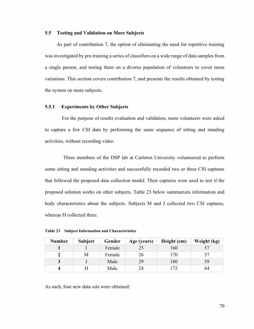
70
5.5 Testing and Validation on More Subjects
As part of contribution 7, the option of eliminating the need for repetitive training
was investigated by pre-training a series of classifiers on a wide range of data samples from
a single person, and testing them on a diverse population of volunteers to cover more
variations. This section covers contribution 7, and presents the results obtained by testing
the system on more subjects.
5.5.1 Experiments by Other Subjects
For the purpose of results evaluation and validation, more volunteers were asked
to capture a few CSI data by performing the same sequence of sitting and standing
activities, without recording video.
Three members of the DSP lab at Carleton University volunteered to perform
some sitting and standing activities and successfully recorded two or three CSI captures
that followed the proposed data collection model. Their captures were used to test if the
proposed solution works on other subjects. Table 23 below summarizes information and
body characteristics about the subjects. Subjects M and J collected two CSI captures,
whereas H collected three.
Table 23 Subject Information and Characteristics
Number Subject Gender Age (years) Height (cm) Weight (kg)
1 I Female 25 160 57
2 M Female 26 170 57
3 J Male 29 180 59
4 H Male 24 172 64
As such, four new data sets were obtained:

71
1) a data set containing the data collected by subject M;
2) a data set containing the data collected by subject J;
3) a data set containing the data collected by subject H; and
4) a data set combining the data collected by the three other subjects (the “other”
data set), at random room locations, with the transmitter mounted at the
ceiling.
Subject M’s data set contained 137 samples before applying class balancing, and
371 after. Subject J’s data set contained 136 samples before applying class balancing, and
359 after. Subject H’s data set contained 177 samples before applying class balancing, and
500 after. The “other” data set contained 450 samples before applying class balancing, and
1,216 after.
Appendix E presents samples of the signals produced by having different subjects
perform the same sequence of sitting and standing activities. It shows how the pattern in
CSI captures is influenced by the body characteristics of the subjects.
5.5.2 Dependence of Classification Performance on Subjects
To study the influence of subject body characteristics on the classification
performance, the classifiers were trained on the data sets acquired by individual subjects.
As shown in Table 24, some classifiers were influenced as they performed differently on
the different data sets. For example, the quadratic discriminant analysis method performed
relatively different for each data set. It achieved an accuracy of 67.7% for subject M, 33.4%
for subject J, 99.4% for subject H, and 89.7% for the combined data set. Most classifiers
performance degraded for the combined data set, which is expected as it is larger in size.

72
Table 24 Classification Results for Individual Subjects, Dependent on the Subject
Classification
Method Type
Accuracy (%)
Subject
M
Subject
J
Subject
H
Subject M, J, H
Combined
Decision Trees
(DTs)
Fine 93.5 95.3 97.4 90.5
Medium 93.5 95.3 97.4 87.0
Coarse 89.5 87.7 88.6 74.1
Discriminant
Analysis (DA)
Linear 83.8 87.5 87.4 72.9
Quadratic 67.7 33.4 99.4 89.7
Naïve Bayes
(NB)
Gaussian Failed Failed 99.4 89.7
Kernel 99.5 99.4 100 95.3
Support Vector
Machines
(SVMs)
Linear 95.4 96.1 98.2 92.2
Quadratic 98.4 97.2 99.2 97.1
Cubic 97.6 97.5 99.2 97.4
Fine Gaussian 94.3 91.1 98.8 90.4
Medium Gaussian 100 100 100 99.8
Coarse Gaussian 90.0 95.5 95.2 88.2
K-Nearest
Neighbours
(KNN)
Fine 80.9 81.9 86.8 82.8
Medium 72.0 69.4 74.0 71.7
Coarse 66.8 63.0 66.2 60.9
Cosine 84.9 93.6 95.2 88.6
Cubic 71.4 70.5 72.4 71.1
Weighted 71.7 68.5 74.0 71.5
Ensemble
Classifiers
Boosted Trees 33.7 33.4 33.6 94.0
Bagged Trees 95.1 98.6 98.2 97.0
Subspace
Discriminant 92.5 92.5 98.2 93.0
Subspace KNN 84.9 86.6 93.4 88.1
RUSBoosted Trees 33.7 45.1 33.6 87.3
The medium Gaussian SVM outperformed the other classifiers by achieving
perfect performances for all subjects, and 99.8% on the combined data set. However, these
variations can be caused by other factors such as activity location, environmental changes,
and noise level as well. Another factor is the integrity of the data collected by the other
subjects as one cannot guarantee that they performed the required exercise as expected. If

73
one can verify that these differences were really caused by individual body characteristics,
that would mean that the system needs to either be repeatedly trained and configured for
users upon deployment (subject dependence), or be trained on a huge data set collected by
a diverse population of subjects (subject independence). The first option would lead to a
system in which the performance depends on the subject; while the second option would
lead to a system in which the performance is independent of the subject.
Tables 25, 26, 27 and 28 show the confusion matrices of the predictions for the
data sets collected by subject M, subject J, subject H, and the combined data set,
respectively.
Table 25 Confusion Matrix Summarizing the Medium Gaussian SVM Predictions for the Data Set
Collected by Subject M
Tru
e C
lass
Still 123 0 0
Sitting-down 0 125 0
Standing-up 0 0 123
Still Sitting-down Standing-up
Predicted Class
Table 26 Confusion Matrix Summarizing the Medium Gaussian SVM Predictions for the Data Set
Collected by Subject J
Tru
e C
lass
Still 120 0 0
Sitting-down 0 119 0
Standing-up 0 0 120
Still Sitting-down Standing-up
Predicted Class

74
Table 27 Confusion Matrix Summarizing the Medium Gaussian SVM Predictions for the Data Set
Collected by Subject H
Tru
e C
lass
Still 166 0 0
Sitting-down 0 166 0
Standing-up 0 0 168
Still Sitting-down Standing-up
Predicted Class
Table 28 Confusion Matrix Summarizing the Medium Gaussian SVM Predictions for the “other”
Data Set, Combining Data Collected by Subjects M, J, and H
Tru
e C
lass
Still 407 2 0
Sitting-down 0 140 0
Standing-up 0 0 640
Still Sitting-down Standing-up
Predicted Class
As the accuracies suggest, the confusion matrices also reflect perfect classification
performances for the data sets of the three subjects, and an almost perfect performance for
the combined data set. All samples were correctly classified for subject M, J, and H. Only
two samples of the combined data set were wrongly classified.
5.5.3 Independence of Classification Performance from Subjects
The classifiers were trained on a data set combining all of the collected data: the
“floor”, “ceiling”, “floor + ceiling”, and “other” data sets. To see how the classifiers would
perform on the data set collected by the volunteers, training the classifiers on it was
considered as well. This was done to aim towards a trained-once activity recognition and

75
monitoring system, which would be able to classify the CSI data corresponding to ADLs,
under any circumstances.
Table 29 Classification Results of Training of Different Data Sets, Independent of the Subject
Classification
Method Type
Accuracy (%)
Floor Ceiling Floor +
Ceiling Other
All
Combined
Decision
Trees (DTs)
Fine 68.1 65.7 64.4 90.5 62.7
Medium 62.5 59.2 59.1 87.0 57.3
Coarse 56.3 55.0 55.2 74.1 54.8
Discriminant
Analysis (DA)
Linear 54.8 54.2 52.5 72.9 52.4
Quadratic 61.1 60.1 58.2 89.7 57.5
Naïve Bayes
(NB)
Gaussian 61.1 60.1 58.2 89.7 57.5
Kernel 72.2 72.6 68.7 95.3 68.5
Support
Vector
Machines
(SVMs)
Linear 67.0 65.9 62.4 92.2 62.2
Quadratic 94.5 93.3 92.2 97.1 92.1
Cubic 97.6 96.6 97.0 97.4 97.0
Fine
Gaussian 90.8 88.6 90.2 90.4 89.8
Medium
Gaussian 98.4 97.6 97.7 99.8 97.6
Coarse
Gaussian 70.7 68.7 66.7 88.2 67.1
K-Nearest
Neighbours
(KNN)
Fine 80.9 80.0 79.7 82.8 79.6
Medium 72.3 71.2 71.5 71.7 71.2
Coarse 57.2 55.3 56.8 60.9 56.7
Cosine 85.8 84.2 85.5 88.6 85.1
Cubic 71.3 70.1 70.8 71.1 70.5
Weighted 72.1 71.6 71.2 71.5 71.1
Ensemble
Classifiers
Boosted
Trees 66.2 63.0 61.0 94.0 60.3
Bagged Trees 96.0 94.8 94.6 97.0 94.3
Subspace
Discriminant 64.5 63.7 59.1 93.0 59.4
Subspace
KNN 86.8 84.8 85.2 88.1 85.0
RUSBoosted
Trees 63.5 60.6 59.8 87.3 58.2

76
Table 29 summarizes the classification accuracies achieved by training the
classifiers on the different data sets (see section 5.3.1). Note that the reason for the values
in the “Floor”, “Ceiling”, and “Floor + Ceiling” columns to differ slightly from the values
in the previous tables is that this experiment was carried out at a later point in time.
Table 30 Classification Results of Training on “floor” Data Set and Testing on “other” Data Set
Classification
Method Type
Accuracy (%)
Training on
“floor” Data Set
Testing on
“other” Data Set
Decision Trees
(DTs)
Fine 68.1 42.1
Medium 62.5 37.1
Coarse 56.3 42.9
Discriminant
Analysis (DA)
Linear 54.8 42.8
Quadratic 61.1 42.3
Naïve Bayes (NB) Gaussian 61.1 42.3
Kernel 72.2 47.0
Support Vector
Machines (SVMs)
Linear 67.0 33.2
Quadratic 94.5 43.8
Cubic 97.6 39.9
Fine Gaussian 90.8 33.6
Medium Gaussian 98.4 35.2
Coarse Gaussian 70.7 45.0
K-Nearest
Neighbours
(KNN)
Fine 80.9 39.6
Medium 72.3 39.5
Coarse 57.2 34.9
Cosine 85.8 35.6
Cubic 71.3 36.8
Weighted 72.1 39.1
Ensemble
Classifiers
Boosted Trees 66.2 38.0
Bagged Trees 96.0 43.4
Subspace Discriminant 64.5 32.9
Subspace KNN 86.8 40.7
RUSBoosted Trees 63.5 36.9
AVERAGE DIFFERENCE 34.5

77
Table 31 Classification Results of Training on “ceiling” Data Set and Testing on “other” Data Set
Classification Method Type
Accuracy (%)
Training on
“ceiling” Data Set
Testing on
“other” Data Set
Decision Trees (DTs)
Fine 65.7 29.7
Medium 59.2 34.4
Coarse 55.0 44.1
Discriminant
Analysis (DA)
Linear 54.2 43.0
Quadratic 60.1 41.5
Naïve Bayes (NB) Gaussian 60.1 41.5
Kernel 72.6 52.5
Support Vector
Machines (SVMs)
Linear 65.9 36.7
Quadratic 93.3 50.4
Cubic 96.6 50.7
Fine Gaussian 88.6 33.6
Medium Gaussian 97.6 34.4
Coarse Gaussian 68.7 49.1
K-Nearest
Neighbours (KNN)
Fine 80.0 39.7
Medium 71.2 37.1
Coarse 55.3 32.5
Cosine 84.2 37.4
Cubic 70.1 36.0
Weighted 71.6 36.8
Ensemble Classifiers
Boosted Trees 63.0 37.9
Bagged Trees 94.8 45.4
Subspace
Discriminant 63.7 33.5
Subspace KNN 84.8 45.9
RUSBoosted Trees 60.6 31.9
AVERAGE DIFFERENCE 32.6
Three sets of models were generated by training the classifiers on the “floor”,
“ceiling”, and “floor + ceiling” data sets, respectively. All models were trained with 5-fold
cross validation to protect the learners against overfitting by partitioning the data sets into
five folds and estimating the classification accuracy on each fold. Afterwards, each of the
78
trained models was tested using the “other” data set, which consisted of the data collected
by the three volunteers, with the receiver on the ground and the transmitter at the ceiling.
Since the activities performed by the other subjects were conducted with the
transmitter mounted at the ceiling, one would expect the testing performance to improve
when training the classifiers on the “ceiling” data set. As can be seen in Tables 30 and 31
above, this was indeed the case. The average difference between the training and testing
accuracies was 34.5% when training on the “floor” data set, while it was reduced to 32.6%
when training on the “ceiling” data set.
In addition, training the classifiers on a larger data set, combining both the “floor”
and “ceiling” data sets reduced the average difference even more. When training on the
“floor + ceiling” data set, the average difference between the training and testing accuracies
was approximately 30.1% (see Table 32 below).
As observed in Tables 30, 31, and 32 above, the performance of the classifiers
significantly dropped when tested on the data set collected by other subjects. These changes
in performance can be due to a number of reasons, including signal/time drift, subject bias,
and classifier overfitting. Factors such as time, environmental changes, noise, and device
calibration contribute to signal drift. On the other hand, the system appeared unable to
detect sitting-down and standing-up actions by different people, which it was not trained
on. Looking closely at the models exported from MATLAB’s Classification Learner, the
prediction functions, used to predict the classes of test data samples, were noticed to
generate ahead of validation, meaning that the system would not be protected against
overfitting.

79
Table 32 Classification Results of Training on “floor + ceiling” and Testing on “other” Data Set
Classification
Method Type
Accuracy (%)
Training on “floor
+ ceiling” Data Set
Testing on
“other” Data Set
Decision
Trees (DTs)
Fine 64.4 33.3
Medium 59.1 37.8
Coarse 55.2 45.0
Discriminant
Analysis (DA)
Linear 52.5 43.8
Quadratic 58.2 43.1
Naïve Bayes
(NB)
Gaussian 58.2 43.1
Kernel 68.7 53.7
Support
Vector
Machines
(SVMs)
Linear 62.4 33.5
Quadratic 92.2 54.4
Cubic 97.0 50.3
Fine Gaussian 90.2 33.6
Medium Gaussian 97.7 39.5
Coarse Gaussian 66.7 50.1
K-Nearest
Neighbours
(KNN)
Fine 79.7 41.0
Medium 71.5 38.7
Coarse 56.8 31.7
Cosine 85.5 41.0
Cubic 70.8 37.3
Weighted 71.2 38.7
Ensemble
Classifiers
Boosted Trees 61.0 39.0
Bagged Trees 94.6 51.2
Subspace Discriminant 59.1 33.1
Subspace KNN 85.2 46.1
RUSBoosted Trees 59.8 37.0
AVERAGE DIFFERENCE 30.1

80
5.5.4 Deep Learning Results
This section will cover contribution 8 from the list of contributions in section 1.4.
Contribution 8 is related to the implementation of a deep learning neural network to
recognize and classify sitting and standing activities. Two versions of the data in the “floor
+ ceiling” data set were generated. One before segmentation (180 samples/sequences), and
another after segmenting the data into 20-packet segments (12,057 samples/sequences).
The first version is useful for testing a sequence-to-sequence model of the network, where
the network takes a time series as the input and outputs a sequence of labels (i.e.
predictions). The inputted time series consisted of the acquired and preprocessed 90-second
CSI signals. The second version of the data is useful for testing a sequence-to-label model
of the designed network, where the network takes a time series as the input and outputs a
label at each iteration. In this case, the inputted time series consisted of the preprocessed
and segmented 1-second CSI signals.
In some real cases, different people may perform the same activity differently. For
all supervised learning, if activities performed by a subject “A” do not appear in training,
the data collected by “A” will be harder to predict during testing. To verify this, the
proposed network was trained with the data collected by one person and validate it with
the data collected by three other subjects. The training data set was collected by one subject,
who performed many variations of sitting and standing speeds and styles.
The network was tested by training and validating it using three activity classes,
and four activity classes. Both seated and standstill activities were first joined into the
“still” class, and both sitting-down and standing-up activities were kept in their respective
classes. Then, the still activities were split into two classes: “seated” and “standstill”. This

81
resulted with four activity classes: “seated”, “standstill”, “sitting-down”, and standing-up”.
Both seated and standstill activities are very similar in the sense that they are stationary.
On the other hand, both sitting-down and standing-up movements contain the same actions
in reverse order. Therefore, it is essential to distinguish among them.
5.5.4.1 Sequence-to-Sequence BiLSTM Network
A sequence-to-sequence model of the BiLSTM network, where the network
takes a time series as the input and outputs a sequence of labels (i.e. predictions) was
explored. The inputted time series consisted of the acquired and preprocessed 90-second
CSI signals. Dealing with the data without segmentation provides a data set of 90-second
sequences. By setting the maximum number of epochs to 100, with a minimum batch size
of 20, having a data set of 180 sequences, each epoch will consist of nine iterations, for a
total of 900 training iterations. The validation data set, on the other hand, contains only
seven sequences.
For the scenario with three activity classes, this model of the BiLSTM network
achieved a classification accuracy of 85.1%. It achieved a classification accuracy of 75.7%
with four activity classes.
5.5.4.2 Sequence-to-Label BiLSTM Network
A sequence-to-label model of the BiLSTM network, where the network takes a
time series as the input and outputs a label at each iteration was explored. In this case, the
inputted time series consisted of the preprocessed and segmented 1-second CSI signals.
The CSI signals were segmented into 20-packet windows and accordingly labelled. A
window length of 20 was chosen because some sitting-down and standing-up activities take

82
about 1 second (i.e. about 20 packets) to complete. To segment the signals, the starting
point for each activity in the sequence was first identified. Once the appropriate starting
timestamp/packet for an activity was located, the signal was segmented into 20-packet
segments until the next event’s timestamp was reached.
Data segmentation split the CSI sequences into 20-packet (1-second) sequences;
thus, providing a much larger data set. By setting the maximum number of epochs to 100,
with a minimum batch size of 20, having a data set of 12,057, each epoch will consist of
602 iterations, for a total of 60,200 training iterations. The validation data set, on the other
hand, contains 450 sequences.
For the scenario with three activity classes, the BiLSTM network achieved a
classification accuracy of 90.7%. For the scenario with four activity classes, the BiLSTM
network achieved a classification accuracy of 55.6%. Since accuracy is not a good measure
of classification performance in the case of imbalanced classes, Table 33 and Table 34
show the confusion matrices as they are more representative of the performance. Table 33
displays the confusion matrix for predicting three classes of activities, while Table 34
displays the confusion matrix for predicting four classes of activities.
Table 33 Confusion Matrix Displaying the Validation Predictions of a Sequence-to-Label BiLSTM
Network, with Three Activity Classes
Tru
e C
lass
Still 407 0 2
Standing-up 20 0 0
Still 19 0 1
Still Sitting-down Standing-up
Predicted Class

83
Table 34 Confusion Matrix Displaying the Validation Predictions of a Sequence-to-Label BiLSTM
Network, with Four Activity Classes
Tru
e C
lass
Seated 182 0 2 57
Sitting-down 11 1 1 8
Standing-up 16 0 2 2
Standstill 101 0 2 65
Seated Sitting-down Standing-up Standstill
Predicted Class
Due to the nature of the employed data collection, the collected data contained
more samples belonging to the “still”, “seated”, and “standstill” classes, and, as such, the
data set was imbalanced. As balancing the classes in time series data can become complex,
and due to time constraints, this item was left for future work. The above confusion
matrices show that the network is affected by the highly imbalanced structure of the
training set. This could also be due to the size of the training set as it deep learning networks
usually need significantly more data to train, or the proposed technique is not suitable for
the problem. Table 35 summarizes all of the obtained results. The sequence-to-label model
achieves a maximum accuracy of 90.7% at recognizing three activity classes: still, sitting-
down, and standing-up.
Table 35 Summary of Results from Both Sequence-to-Sequence and Sequence-to-Label Models of
the BiLSTM Network
Test
Implementation Details
Model Training
Samples
Testing
Samples
Activity
Classes
Accuracy
(%)
1 Sequence-to-Sequence 180 7 3 85.1
2 Sequence-to-Sequence 180 7 4 75.7
3 Sequence-to-Label 12,057 450 3 90.7
4 Sequence-to-Label 12,057 450 4 55.6

84
Chapter 6: Conclusion
This chapter concludes the thesis with a discussion of the main research findings and
includes some closing remarks and possible extensions of the work.
6.1 Summary of Related Work
This thesis utilizes the Wi-Fi devices provided by Aerial Technologies, as in [1, 33],
and proposes a HAR system that could potentially be used to recognize ADLs. It extends
the previous application of Wi-Fi CSI analysis for motion and location detection to not
only distinguish between a no motion activity and motion activities, as it is the case in [33],
but to also allow for two very similar motions of standing-up and sitting-down to be
distinguished from one another. The sensor used in [33] was simply a motion detector,
while this thesis introduces a HAR sensor that can capture movement/motion patterns.
Although [42 - 47] distinguish among ADL, [42, 43] do not distinguish between similar
movements, and only [44, 47] apply deep learning.
This work focuses on the recognition of the two similar dynamic motions of sitting-
down and standing-up. Furthermore, [42 - 47] apply more complex preprocessing
algorithms. This thesis aims at simplifying the preprocessing methodology, while still
achieving an acceptable recognition/classification performance. The applied feature
extraction and traditional machine learning classification, in this work, have demonstrated
the ability to extend the previous application of Wi-Fi CSI analysis for motion and location
detection to not only distinguish between a no motion activity and two motion activities,
but to also allow for two very similar motions of standing-up and sitting-down to be
distinguished from one another.

85
Traditional machine learners as well as a deep learning network were tested to
classify sitting and standing activities. Table 36 compares the performance achieved by
this work, at recognizing sitting and standing activities, with some state-of-the-art studies.
The top three rows of the table represent the results presented in this thesis, and the support
papers in comparison to other works.
Table 36 Comparison of Classification Performances with Related Work
Reference Movement Classification Method Average Accuracy (%)
New [1] Dynamic Traditional Machine Learning 98.4
New Dynamic Traditional Machine Learning 98.2
New Dynamic Deep Learning 87.9
[42] Static Traditional Machine Learning 92
[43] Static Traditional Machine Learning 96
[44] Dynamic Deep Learning over 80
[45] Dynamic Traditional Machine Learning 92
[46] Dynamic Traditional Machine Learning 95.3
[47] Dynamic Deep Learning 97
6.2 Discussion of Results
CSI data were acquired by performing a sequence of still, sitting-down and standing-
up action activities, preprocessed the acquired signals, extracted features, and labelled the
data samples for traditional, supervised machine learning. Four different data sets were
generated using the acquired Wi-Fi CSI signals: “preliminary”, “floor”, “ceiling”, and
“floor + ceiling” (see section 5.3.1). The “preliminary” data set contained data collected by
a single subject, at a single room location, with both Wi-Fi devices placed on the ground.
The so-called “preliminary” data set was utilized to perform basic test cases for the
proposed contributions. The “floor” data set contained data collected by a single subject,
at various room locations, with both Wi-Fi devices placed on the floor. The “ceiling” data

86
set included data collected by a single subject, at various room locations, with one Wi-Fi
device mounted at the ceiling and the other placed on the floor. The “floor + ceiling” data
set simply combined both of the “floor” and “ceiling” data sets together.
MATLAB’s Classification Learner was used to train various classifiers on the CSI
data (see section 4.5.1). The classifiers were trained and tested using 5-fold cross
validation. Basic tests, with minimal data preprocessing (only filtering), were performed
on the so-called “preliminary” data set. As such, the medium Gaussian SVM achieved a
highest accuracy of 98.4%. The manner at which SVMs operate explains the obtained
results. SVMs determine an optimal hyperplane that defines a clear gap between the data
points in terms of space [48].
As part of data preprocessing, the effects of standardizing/normalizing the CSI
measurements and scaling the extracted features, on classification accuracies, were studied
(see section 5.2). The medium Gaussian SVM achieved a highest accuracy of 98.8% for
the so-called “preliminary” data set, by applying z-score standardization over subcarrier
indices for each timestamp/packet, and scaling the features at all levels of the feature
extraction paradigm.
By testing and reporting results on the “floor”, “ceiling”, and “floor + ceiling” data
sets, different activity locations and device placements were examined (see section 5.3).
The best classification performance was achieved by training the classifiers on the “floor”
data set. The medium Gaussian SVM achieved an accuracy of 98.5% for the “floor” data
set, 97.7% for the “ceiling” data set, and 97.8% for the “floor + ceiling” data set. The
proposed solution was able to successfully distinguish between the three cases: stationary

87
activities such as remaining seated or standstill, and two dynamic activities such as sitting-
down or standing-up that were performed by one person. This goes beyond detecting
motion as the system was able to distinguish between two different movements.
Time repeatability and drift were also tested (see section 5.4) by running the
classifiers on data sets collected on different days (“day 1” and “day 2”), and again on data
sets collected on the same day, within a short period of time (“capture 1” and “capture 2”).
In terms of repeatability, the obtained results showed that the proposed solution performed
as good, regardless of the time/date the tests and data collection. In terms of drift, the
obtained results showed that the proposed solution was influenced by drift and/or other
factors. The classification performance of the system degraded when training it on one data
set, with 5-fold cross validation, and testing it on another data set. The performance was
degraded despite the amount of time passed between the collection of the two data sets.
Most of the acquired CSI data were captured by a single person performing the
proposed sequence of sitting-down and standing-up activities, using various experimental
setups. More data were collected by other subjects to cover different variations of age,
gender, height, and weight. Other means of validation, such as holdout validation and
separate testing data sets, were also investigated to see to what extent can the system
proceed without degrading the performance. The different classifiers were trained on data
collected by the preliminary subject (the author), and tested using data collected by other
subjects. This was done in an effort to explore the user independence of the proposed
methods. Unfortunately, the classification performance was significantly degraded when
training the classifiers on the data collected by one subject and testing on the data collected
by other subjects. This can be a result of many factors, such as overfitting the training data,
88
time/signal drifting, environmental changes, or the differing body characteristics of
subjects. Another issue that comes into question is the integrity of the data collected by the
other subjects, as one cannot guarantee that they precisely followed the experimental
instructions. Thus, the resulting CSI signals might be largely affected and not similar, in
pattern, to those that were used during the training process.
A BiLSTM network was designed to perform deep learning on the acquired Wi-Fi
CSI data (see section 4.5.2 and 5.5.4). The network was tested for both sequence-to-
sequence and sequence-to-label models of classification. The inputted sequences were
constituted of time series of 21 attributes. Furthermore, the two models were tested using
three activity classes (still, sitting-down, and standing-up), as well as four activity classes
(seated, standstill, sitting-down, and standing-up). The seated and standstill activities are
static, while sitting-down and standing-up are dynamic activities.
The sequence-to-sequence model was trained on 180 labelled time series, and tested
on seven time series. In this scenario, the network achieved a validation accuracy of 85.1%
at classifying sitting and standing sequences, with three activity classes. It achieved a
validation accuracy of 75.7% at classifying sitting and standing sequences, with four
activity classes.
The sequence-to-label model was trained on 12,057 labelled time series, and tested
on 450 time series. In this scenario, the network achieved a validation accuracy of 90.7%
at classifying sitting and standing sequences, with three activity classes. It achieved a
validation accuracy of 55.6% at classifying sitting and standing sequences, with four
activity classes.
89
The classification performance is expected to increase if the BiLSTM network was
to be trained on a larger amount of data. Also, due to the data collection process, there is a
class imbalance, where the still activities are majority, which could influence the
classification performance. Since the nature of BiLSTM requires ordered data and most
current approaches for data balancing do not provide solutions that maintain the order of
data, the class imbalance issue will have to be studied in more detail and addressed as part
of future work.
6.3 Future Work
In general, Wi-Fi seems an appropriate solution for capturing movements and non-
still activities. The proposed solution performs well on data that it was trained on, with 5-
fold cross validation, and data similar to the one that it was trained on, but not on data
collected at other times or by other subjects. The performance of the system is then said to
be user dependent, meaning that it would need to be continually trained in an adaptive
machine learning process. In future work, the solution should improve in terms of subject
dependence and independence from classification performance, by collecting more diverse
data sets.
In the future, the addition of a stateful mechanism will be explored to improve the
classification by distinguishing between standing still and seated, by tracking previous
predictions to decide whether the subject is sitting still or standing still © 2019 [1]. If the
mechanism detects that the person was standing-up before, he/she is likely standing still
after. Also, one should aim towards recognizing other human activities such as walking.
Finally, as part of future work, the potential for a hybrid classifier that combines the results
from multiple classifiers will be explored to predict activities by favouring the most

90
predicted class among all classifiers in order to potentially achieve an improved
performance.

91
Appendices
Appendix A Summary of Data Samples
This appendix contains a table summary of all of the conducted experiments, which
provided the data for this work.
Table 37 Summary of Sitting and Standing Data Samples Collected under a 2D (Ground-Ground)
Device Placement, by the Author
Device Location Activity
Location
Body
Orientation
Sit-Stand Style/Speed Total
AP STA 1 2 3
Ground Ground Middle
Front 2 2 3 7
Back 2 2 3 7
Towards AP 3 2 3 8
Towards STA 3 2 2 7
Left 2 2 2 6
Right 2 2 3 7
Ground Ground Near AP
Front 1 1 1 3
Back 1 1 1 3
Towards AP 1 1 1 3
Towards STA 1 1 1 3
Left 1 1 1 3
Right 1 1 1 3
Ground Ground Near STA
Front 1 1 1 3
Back 1 1 1 3
Towards AP 1 1 1 3
Towards STA 1 1 1 3
Left 1 1 1 3
Right 1 1 1 3
Ground Ground Front-Left
Corner
Front 1 1 1 3
Back 1 1 1 3
Left 1 1 1 3
Right 1 1 1 3
Ground Ground Back-Right
Corner
Front 1 1 1 3
Back 1 1 1 3
Left 1 1 1 3
Right 1 1 1 3
TOTAL NUMBER OF DATA SAMPLES 34 32 36 102

92
Table 38 Summary of Sitting and Standing Data Samples Collected under a 3D (Ceiling-Ground)
Device Placement, by the Author
Device Location Activity
Location
Body
Orientation
Number of Samples per
Sit-Stand Style/Speed Total
AP STA 1 2 3
Ceiling Ground Middle
Front 1 1 1 3
Back 1 1 1 3
Towards AP 1 1 1 3
Towards STA 1 1 1 3
Left 1 1 1 3
Right 1 1 1 3
Ceiling Ground Near AP
Front 1 1 1 3
Back 1 1 1 3
Towards AP 1 1 1 3
Towards STA 1 1 1 3
Left 1 1 1 3
Right 1 1 1 3
Ceiling Ground Near STA
Front 1 1 1 3
Back 1 1 1 3
Towards AP 1 1 1 3
Towards STA 1 1 1 3
Left 1 1 1 3
Right 1 1 1 3
Ceiling Ground Front-Left
Corner
Front 1 1 1 3
Back 1 1 1 3
Left 1 1 1 3
Right 1 1 1 3
Ceiling Ground Back-Right
Corner
Front 1 1 1 3
Back 1 1 1 3
Left 1 1 1 3
Right 1 1 1 3
TOTAL NUMBER OF DATA SAMPLES 26 26 26 78
Table 39 Summary of Sitting and Standing Data Samples Collected by Three Volunteer Subjects
Device Location Activity
Location
Body
Orientation
Number of Samples
by Subject Total
AP STA M J H
Ceiling Ground Random Random 2 2 3 7

93
Table 40 Summary of Additional Data Samples Collected by the Author, but Not Used
Device Location Activity/Chair
Location
Body
Orientation Activity
Number
of
Samples
Total AP STA
Ground Ground
Middle Front/Back/Left Seated 6 6
Middle Front/Back/Left Standstill 6 6
Middle N/A
Empty
Room
3
6
Near Receiver N/A 1
Front-Left
Corner N/A 1
Back-Right
Corner N/A 1
Middle Random
Walking
back and
fourth
across the
room
3 3
Ceiling Ground
Middle Front/Back/Left Seated 1 1
Middle Front/Back/Left Standstill 1 1
Middle N/A
Empty
Room
1
5
Near
Transmitter N/A 1
Near Receiver N/A 1
Front-Left
Corner N/A 1
Back-Right
Corner N/A 1
TOTAL NUMBER OF DATA SAMPLES 28

94
Appendix B Samples of Preprocessed Data
This appendix includes figures displaying and comparing samples of the data produced by
different processing techniques. This appendix is to presents how the pattern in one CSI
capture changes depending on the applied preprocessing technique(s). Although the
evident pattern in sole preprocessing methods, containing a singly preprocessing technique
(filtering, normalization, or feature scaling) was destroyed when applying a combination
of methods (see Figure 23 in Appendix B.5), the combined preprocessing approach
optimized the classification performance.
B.1 Raw Signal
Figure 14 Sample Plots of a Raw Signal

95
B.2 Filtering
Figure 15 Sample Plots of a Filtered Signal

96
B.3 Normalization
Z-Score Standardization
Over Time
Figure 16 Sample Plots of Signals Normalized via Z-Score Standardization, over the Time/Packet
Domain

97
Over Subcarriers
Figure 17 Sample Plots of Signals Normalized via Z-Score Standardization, over the Subcarriers
Domain
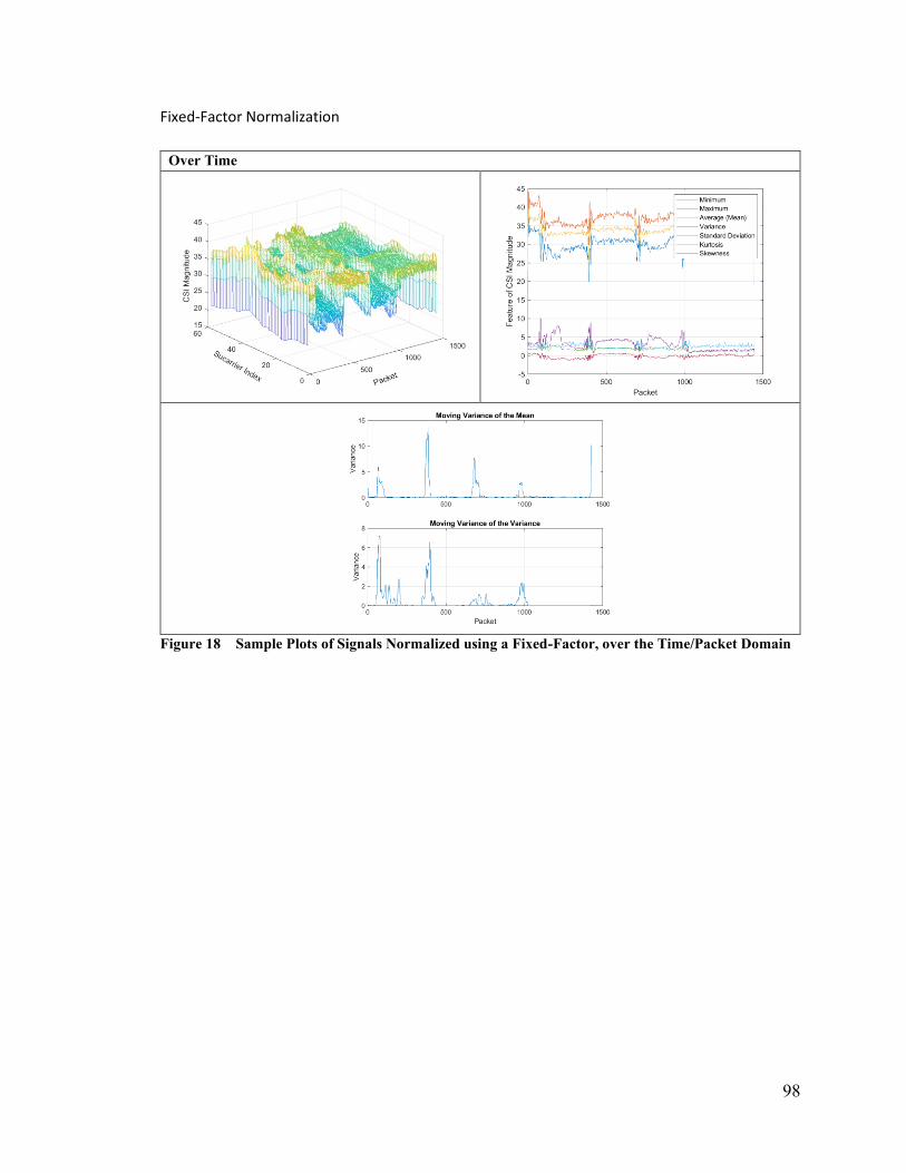
98
Fixed-Factor Normalization
Over Time
Figure 18 Sample Plots of Signals Normalized using a Fixed-Factor, over the Time/Packet Domain

99
Over Subcarriers
Figure 19 Sample Plots of Signals Normalized using a Fixed-Factor, over the Subcarriers Domain

100
B.4 Feature Scaling
Subcarrier Features
Figure 20 Sample Plots of Signals Scaled through Subcarrier Features

101
Time Features
Figure 21 Sample Plots of Signals Scaled through Time Features

102
All Features
Figure 22 Sample Plots of Signals Scaled through Both Subcarrier and Time Features

103
B.5 Filtering, Z-Score Standardization, and Feature Scaling Combined
Figure 23 Sample Plots of Filtered, Z-Score Standardized (over subcarriers), and Scaled (all
features) Signals

104
Appendix C Samples of Data from Different Activity Locations
This appendix includes figures representing data samples collected at different locations
around the laboratory.
C.1 Middle
Figure 24 Sample Plots of Data Collected at the Middle of a Room

105
C.2 Near the Transmitter
Figure 25 Sample Plots of Data Collected near the Transmitter

106
C.3 Near the Receiver
Figure 26 Sample Plots of Data Collected near the Receiver

107
C.4 Empty Corners
Front-Left Corner
Figure 27 Sample of Plots of Data Collected at the Empty Front-Left Corner of a Room

108
Back-Right Corner
Figure 28 Sample of Plots of Data Collected at the Empty Back-Right Corner of a Room

109
Appendix D Samples of Data with Different Device Placements
This appendix includes figures displaying data samples collected with differing device
placements.
D.1 2D (Ground-Ground) Device Placement
Figure 29 Sample of Plots with Data Collected under a 2D (Ground) Device Placement

110
D.2 3D (Ceiling-Ground) Device Placement
Figure 30 Sample of Plots with Data Collected under a 3D (Ground-Ceiling) Device Placement
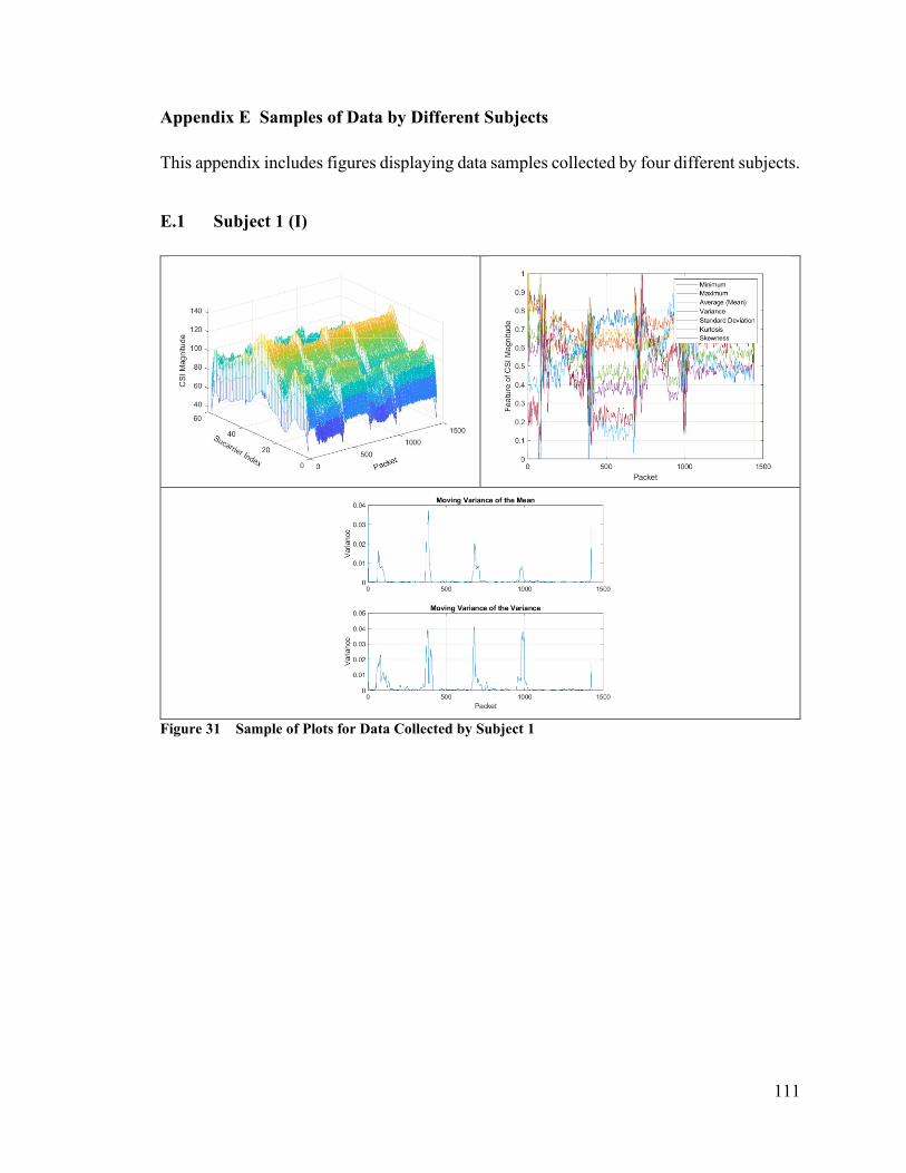
111
Appendix E Samples of Data by Different Subjects
This appendix includes figures displaying data samples collected by four different subjects.
E.1 Subject 1 (I)
Figure 31 Sample of Plots for Data Collected by Subject 1

112
E.2 Subject 2 (M)
Figure 32 Sample of Plots for Data Collected by Subject 2

113
E.3 Subject 3 (J)
Figure 33 Sample of Plots for Data Collected by Subject 3

114
E.4 Subject 4 (H)
Figure 34 Sample of Plots for Data Collected by Subject 4

115
Bibliography or References
[1] I. Joudeh et al, “WiFi Channel State Information-Based Recognition of Sitting-
Down and Standing-Up Activities,” in IEEE International Symposium on Medical
Measurements and Applications (MeMeA), Istanbul, Turkey, 2019.
[2] C. Zhu and W. Sheng, “Realtime Recognition of Complex Human Daily Activities
Using Human Motion and Location Data,” in IEEE Transactions on Biomedical
Engineering, vol. 59, (9), pp. 2422-2430, 2012.
[3] B. Wallace, R. Goubran, and F. Knoefel, “Cognition Assessment: A Framework for
Episodic Measurement,” in IEEE International Symposium on Medical
Measurements and Applications (MeMeA), Benevento, Italy, pp. 1-6, 2016.
[4] B. Wallace et al, “Monitoring cognitive ability in patients with moderate dementia
using a modified “whack-a-mole,” in IEEE International Symposium on Medical
Measurements and Applications (MeMeA), Rochester, MN, USA, 2017.
[5] B. Wallace et al, “Detecting Cognitive Ability Changes in Patients With Moderate
Dementia Using a Modified “Whack-a-Mole” Game,” in IEEE Transactions on
Instrumentation and Measurement (TIM), vol. 67, (7), pp. 1521-1534, 2018.

116
[6] K. K. Htike, O. O. Khalifa, H. A. M. Ramli, and M. A. M. Abushariah, “Human
Activity Recognition for Video Surveillance using Sequences of Postures,” in
International Conference on e-Technologies and Networks for Development
(ICeND2014), Beirut, Lebanon, 2014.
[7] M. K. Fiaz and B. Ijaz, “Vision Based Human Activity Tracking Using Artificial
Neural Networks,” in International Conference on Intelligent and Advanced
Systems, Manila, Philippines, 2010.
[8] O. Bodilovskyi and A. Popov, “Estimation of Time Domain Parameters for
Camera-Based Respiration Monitoring,” in Signal Processing Symposium
(SPSympo), Jachranka, Poland, 2017.
[9] R. Alfuadi and K. Mutijarsa, “Classification Method for Prediction of Human
Activity Using Stereo Camera,” in International Seminar on Application for
Technology of Information and Communication (ISemantic), Semarang, Indonesia,
2016.
[10] X. Cai, G. Han, and J. Wang, “Assessment of Gait Parameters during
Unconstrained Straight-line Walking using a Single Camera,” in IEEE
International Conference on Awareness Science and Technology (iCAST),
Qinhuangdao, China, 2015.

117
[11] K. Song and W. Chen, “Human Activity Recognition Using a Mobile Camera,” in
International Conference on Ubiquitous Robots and Ambient Intelligence (URAI),
Incheon, South Korea, 2011.
[12] M. Z. Uddin, N. D. Thang, and T. Kim, “Human Activity Recognition via 3-D Joint
Angle Features and Hidden Markov Models,” in IEEE International Conference on
Image Processing (ICIP), Hong Kong, China, 2010.
[13] M.W.C.N. Moladande and B.G.D.A. Madhusanka, “Implicit Intention and Activity
Recognition of Human Using Neural Networks for a Service Robot Eye,” in
International Research Conference on Smart Computing and Systems Engineering
(SCSE), Colombo, Sri Lanka, Sri Lanka, 2019.
[14] K. Avgerinakis, K. Adam, A. Briassouli, and Y. Kompatsiaris, “Moving Camera
Human Activity Localization and Recognition with Motionplanes and Multiple
Homographies,” in IEEE International Conference on Image Processing (ICIP),
Quebec City, QC, Canada, 2015.
[15] N. Käse, M. Babaee, and G. Rigoll, “Multi-view Human Activity Recognition using
Motion Frequency,” in IEEE International Conference on Image Processing
(ICIP), Beijing, China, 2017.

118
[16] B. Wallace, T. El Harake, R. Goubran, N. Valech, and F. Knoefel, “Preliminary
Results for Measurement and Classification of Overnight Wandering by Dementia
Patient using Multi-Sensors,” in IEEE International Instrumentation Measurement
Technology Conference (I2MTC), pp. 1-6, 2018.
[17] L. Russell, R. Goubran, and F. Kwamena, “Posture Sensing using a Low-cost
Temperature Sensor Array,” in IEEE International Symposium on Medical
Measurements and Applications (MeMeA), Rochester, MN, USA, pp. 443-447,
2017.
[18] L. Russell, R. Goubran, and F. Kwamena, “Posture Detection Using Sounds and
Temperature: LMS-Based Approach to Enable Sensory Substitution,” in IEEE
Transactions on Instrumentation and Measurement (TIM), vol. 67, (7), pp. 1543-
1554, 2018.
[19] N. A. Capela, E. D. Lemaire, and N. Baddour, “Improving Classification of Sit,
Stand, and Lie in a Smartphone Human Activity Recognition System,” in
Proceedings of IEEE International Symposium on Medical Measurements and
Applications (MeMeA), Torino, Italy, pp. 473-478, 2015.
[20] G. De Leonardis et al, “Human Activity Recognition by Wearable Sensors:
Comparison of Different Classifiers for Real-Time Applications,” in IEEE

119
International Symposium on Medical Measurements and Applications (MeMeA),
Rome, Italy, pp. 1-6, 2018.
[21] A. Lopez, D. Perez, F. J. Ferrero, and O. Postolache, “A Real-Time Algorithm to
Detect Falls in the Elderly,” in IEEE International Symposium on Medical
Measurements and Applications (MeMeA), Rome, Italy, pp. 1-5, 2018.
[22] B. Andò et al, “An event polarized paradigm for ADL detection in AAL context,”
in Proceedings of IEEE International Instrumentation and Measurement
Technology Conference (I2MTC), Montevideo, Uruguay, 2014.
[23] B. Andò, S. Baglio, C. O. Lombardo, and V. Marletta, “An Event Polarized
Paradigm for ADL Detection in AAL Context,” in IEEE Transactions on
Instrumentation and Measurement (TIM), vol. 64, (7), pp. 1814-1825, 2015.
[24] B. Andò, S. Baglio, C. O. Lombardo, and V. Marletta, “A Multisensor Data-Fusion
Approach for ADL and Fall Classification,” in IEEE Transactions on
Instrumentation and Measurement (TIM), vol. 65, (9), pp. 1960-1967, 2016.
[25] Z. Wang et al, “Inertial Sensor-Based Analysis of Equestrian Sports Between
Beginner and Professional Riders Under Different Horse Gaits,” in IEEE
Transactions on Instrumentation and Measurement (TIM), vol. 67, (11), pp. 2692-
2704, 2018.

120
[26] A. Yurtman and B. Barshan, “Novel Non-Iterative Orientation Estimation for
Wearable Motion Sensor Units Acquiring Accelerometer, Gyroscope, and
Magnetometer Measurements,” in IEEE Transactions on Instrumentation and
Measurement (TIM) (Early Access), pp. 1-1, 2019.
[27] S. Matsuguma and A. Kajiwara, “Bathroom accident detection with 79GHz-band
millimeter wave sensor,” in IEEE Sensors Applications Symposium (SAS), Sophia
Antipolis, France, 2019.
[28] T. L. M. van Kasteren, G. Englebienne, and B. J. A. Kröse, “An activity monitoring
system for elderly care using generative and discriminative models,” in Personal
and Ubiquitous Computing, vol. 14, (6), pp 489-498, 2010.
[29] Z. Gu et al, “Blind Separation of Doppler Human Gesture Signals Based on
Continuous-Wave Radar Sensors,” in IEEE Transactions on Instrumentation and
Measurement (TIM), vol. 68, (7), pp. 2659-2661, 2019.
[30] S. K. Leem, F. Khan, and S. H. Cho, “Detecting Mid-air Gestures for Digit Writing
with Radio Sensors and a CNN,” in IEEE Transactions on Instrumentation and
Measurement (TIM) (Early Access), pp. 1-1, 2019.

121
[31] Z. Wang, B. Guo, Z. Yu, and X. Zhou, “Wi-Fi CSI-Based Behavior Recognition:
From Signals and Actions to Activities,” in IEEE Communications Magazine, vol.
56, (5), pp. 109-115, 2018.
[32] Y. Zeng, P. Pathak, and P. Mohapatra, “WiWho: Wifi-based Person Identification
in Smart Spaces,” in Proceedings of the 15th International Conference on
Information Processing in Sensor Networks, pp. 1-12, 2016.
[33] N. Ghourchian, M. Allegue-Martinez, and D. Precup, “Real-Time Indoor
Localization in Smart Homes using Semi-Supervised Learning,” in Proceedings of
the 29th AAAI Conference on Innovative Applications (IAAI-17), pp. 4670-4677,
2017.
[34] D. Alshamaa, A. Chkeir, F. Mourad-Chehade, and P. Honeine, “A Hidden Markov
Model for Indoor Trajectory Tracking of Elderly People,” in IEEE Sensors
Applications Symposium (SAS), Sophia Antipolis, France, 2019.
[35] Q. Gao, J. Wang, X. Ma, X. Feng, and H. Wang, “CSI-Based Device-Free Wireless
Localization and Activity Recognition Using Radio Image Features,” in IEEE
Transactions on Vehicular Technology, vol. 66, (11), pp. 10346-10356, 2017.
122
[36] M. Miyazaki, S. Ishida, A. Fukuda, T. Murakami, and S. Otsuki, “Initial Attempt
on Outdoor Human Detection using IEEE802.11ac WLAN Signal,” in IEEE
Sensors Applications Symposium (SAS), Sophia Antipolis, France, 2019.
[37] J. Liu et al, “Tracking Vital Signs During Sleep Leveraging Off-the-shelf WiFi,” in
Proceedings of the 16th ACM International Symposium on Mobile Ad Hoc
Networking and Computing, pp. 267-276, 2015.
[38] X. Wang, C. Yang, and S. Mao, “PhaseBeat: Exploiting CSI Phase Data for Vital
Sign Monitoring with Commodity WiFi Devices,” in IEEE 37th International
Conference on Distributed Computing Systems (ICDCS), pp. 1230-1239, 2017.
[39] N. Patwari, L. Brewer, Q. Tate, O. Kaltiokallio, and M. Bocca, “Breathfinding: A
Wireless Network That Monitors and Locates Breathing in a Home,” in IEEE
Selected Topics in Signal Processing, vol. 8, (1), pp. 30-42, 2014.
[40] L. Wang, K. Sun, H. Dai, A. X. Liu, and X. Wang, “WiTrace: Centimeter-level
passive gesture tracking using WiFi signals,” in IEEE 15th Annual International
Conference on Sensing, Communication, and Networking (SECON), pp. 1-9, 2018.
[41] K. Ali, A. X. Liu, W. Wang, and M. Shahzad, “Keystroke Recognition Using Wifi
Signals,” in Proceedings of the 21st Annual ACM International Conference on
Mobile Computing and Networking, pp. 90-102, 2015.

123
[42] Y. Wang et al, “E-eyes: Device-free Location-oriented Activity Identification using
Fine-grained WiFi Signatures,” in Proceedings of the 20th Annual International
Conference on Mobile Computing and Networking, pp. 617-628, 2014.
[43] W. Wang, A. X. Liu, M. Shahzad, K. Ling, and S. Lu, “Understanding and
Modeling of WiFi Signal based Human Activity Recognition,” in Proceedings of
the 21st Annual International Conference on Mobile Computing and Networking,
pp. 65-76, 2015.
[44] H. Li, K. Ota, M. Dong, and M. Guo, “Learning Human Activities through Wi-Fi
Channel State Information with Multiple Access Points,” in IEEE Communications
Magazine, vol. 56, (5), pp. 124-129, 2018.
[45] B. Tan et al, “Exploiting WiFi Channel State Information for Residential
Healthcare Informatics,” in IEEE Communications Magazine, vol. 56, (5), pp. 130-
137, 2018.
[46] W. Li, B. Tan, and R. J. Piechocki, “WiFi-based Passive Sensing System for Human
Presence and Activity Event Classification,” in IET Wireless Sensor Systems, vol.
8, (6), pp. 276-283, 2018.

124
[47] Z. Chen, L. Zhang, C. Jiang, Z. Cao, and W. Cui, “WiFi CSI Based Passive Human
Activity Recognition Using Attention Based BLSTM,” in IEEE Transactions on
Mobile Computing, pp. 1-12, 2018.
[48] E. Alpaydin, Introduction to Machine Learning. Cambridge, MA: Massachusetts
Institute of Technology (MIT) Press, 2010.
[49] M. I. Jordan and T. M. Mitchell, “Machine learning: Trends, perspectives, and
prospects,” in Science, vol. 349, (6245), pp. 255-260, 2015.
[50] Y. LeCun, Y. Bengio, and G. Hinton, “Deep learning,” in Nature, vol. 521, (7553),
pp. 436-444, 2015.
[51] Aerial Technologies, “Aerial Solution Setup Guide,” Montreal, QC, 2018.
[52] H. He, Y. Bai, E. A. Garcia, and S. Li, “ADASYN: Adaptive Synthetic Sampling
Approach for Imbalanced Learning,” in Proceedings of IEEE International Joint
Conference on Neural Networks, Hong Kong, China, pp. 1322-1328, 2018.