exploitation of path diversity in cooperative multi-hop wireless networks dissertation committee...
TRANSCRIPT

Exploitation of Path Diversity in Cooperative Multi-Hop Wireless Networks
Dissertation Committee
Department of Electrical and Computing EngineeringUniversity of Delaware
Dr. CiminiDr. CottonDr. ShenDr. Morris
(ECE Department)(ECE Department)(CIS Department)(CERDEC)
CandidateChair
: Jonghyun Kim: Dr. Bohacek

Introduction and challenges Aggressive path quality monitoring
BSP Efficient path quality monitoring
LBSP Opportunistic forwarding
LBSP2, LOSP, LMOSP Conclusion and future work
Outline
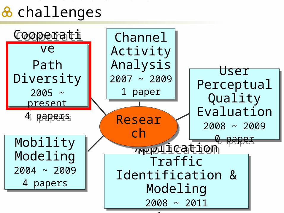
Introduction and challenges
Mobility Modeling2004 ~ 2009
4 papers
Mobility Modeling2004 ~ 2009
4 papers
CooperativePath Diversity
2005 ~ present4 papers
CooperativePath Diversity
2005 ~ present4 papers
Channel Activity Analysis
2007 ~ 20091 paper
Channel Activity Analysis
2007 ~ 20091 paper
User Perceptual Quality
Evaluation2008 ~ 2009
0 paper
User Perceptual Quality
Evaluation2008 ~ 2009
0 paper
Application Traffic Identification & Modeling
2008 ~ 20111 paper
Application Traffic Identification & Modeling
2008 ~ 20111 paper
ResearchResearch

Routing Technique
Proactive(e.g., OLSR)
Reactive(e.g., AODV)
Introduction and challenges
Introduction and challenges
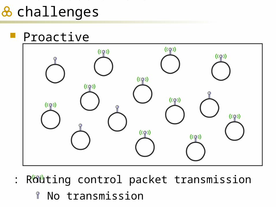
: Routing control packet transmission
: No transmission
Proactive
Introduction and challenges
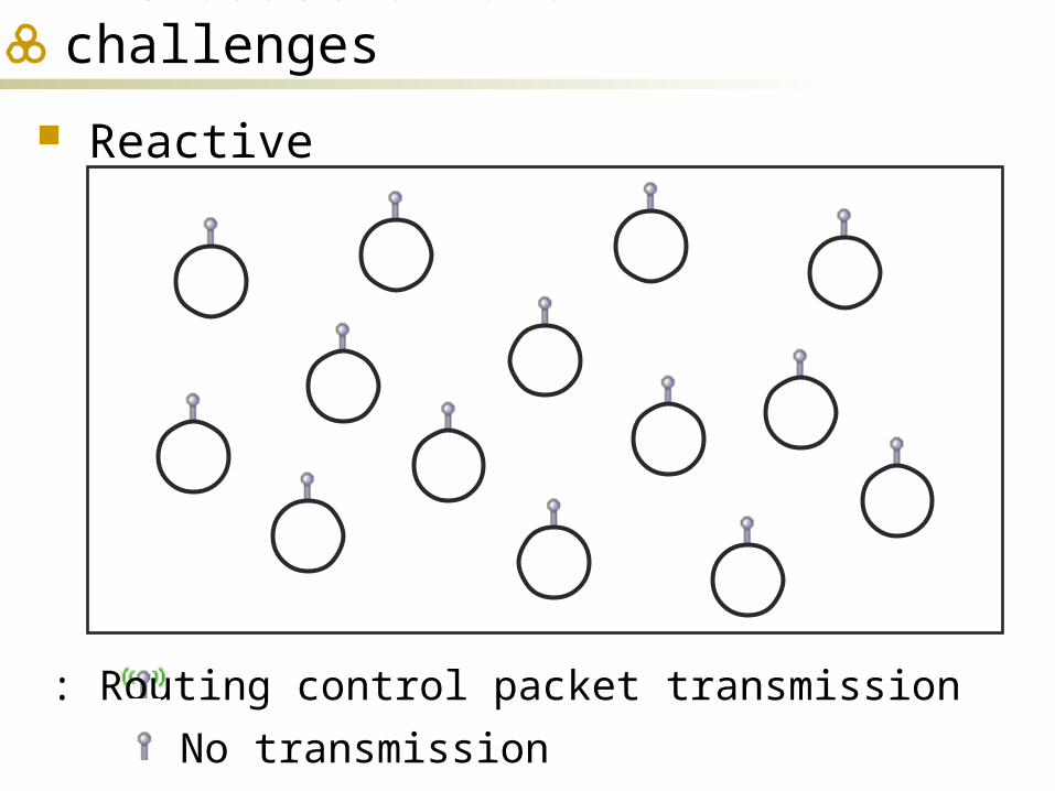
: Routing control packet transmission
: No transmission
Reactive

Introduction and challenges
: data packet from transport layer
Reactive
Introduction and challenges
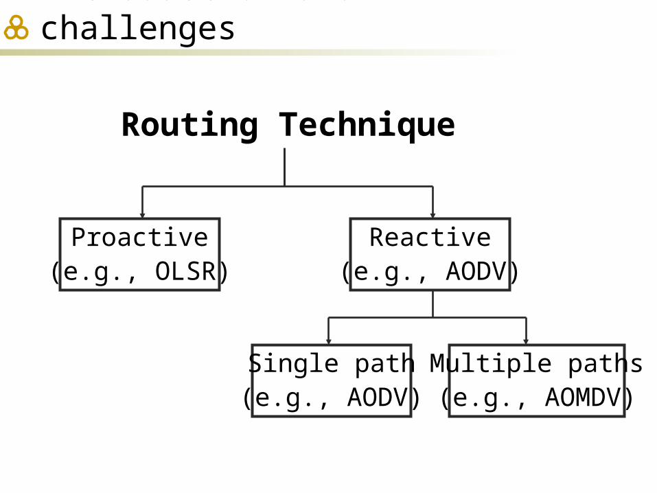
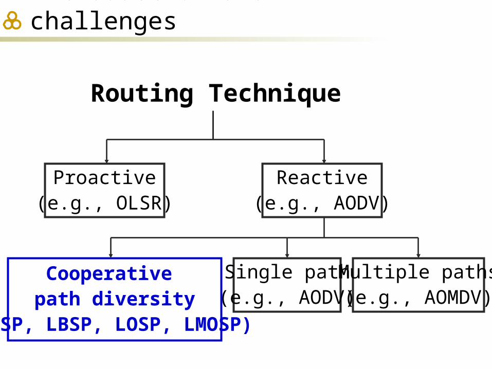
Routing Technique
Proactive(e.g., OLSR)
Reactive(e.g., AODV)
Single path(e.g., AODV)
Multiple paths(e.g., AOMDV)
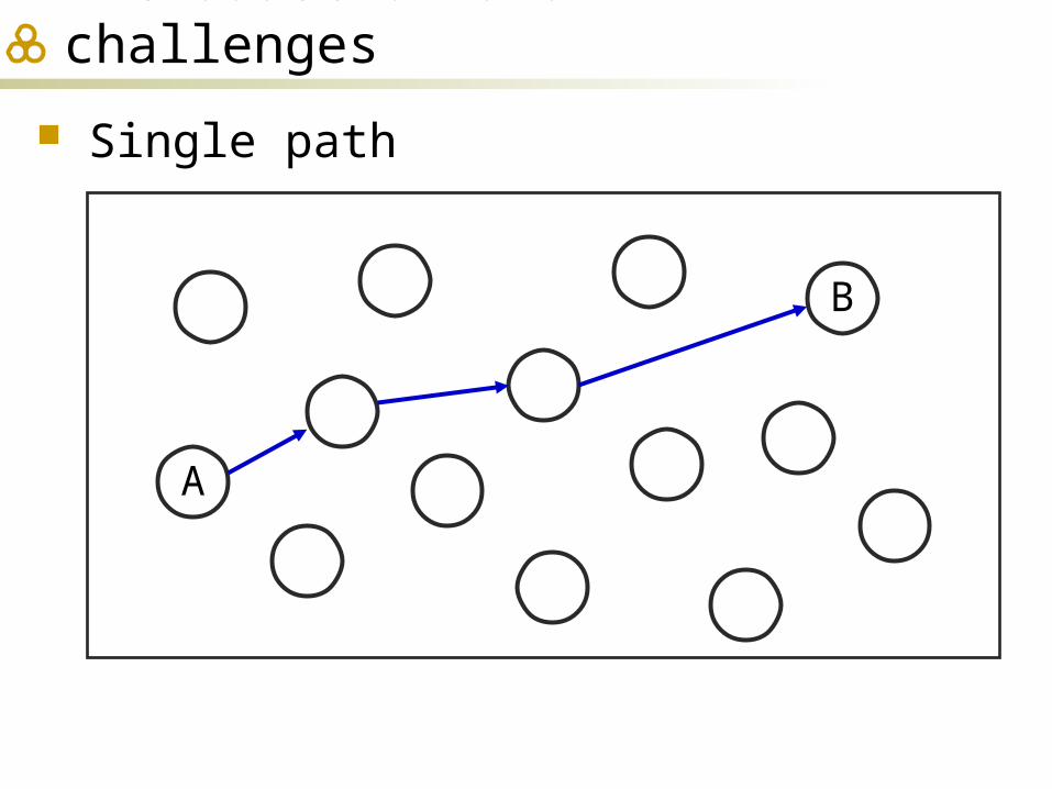
Introduction and challenges
Single path
B
A

Introduction and challenges
Multiple paths
B
A
Introduction and challenges
Routing Technique
Proactive(e.g., OLSR)
Reactive(e.g., AODV)
Single path(e.g., AODV)
Multiple paths(e.g., AOMDV)
Cooperative path diversity
(BSP, LBSP, LOSP, LMOSP)
Cooperative path diversity
BA
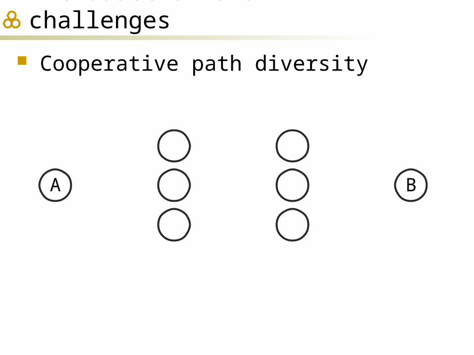
Introduction and challenges
Cooperative path diversity
BA
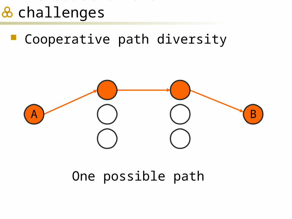
One possible path
Introduction and challenges
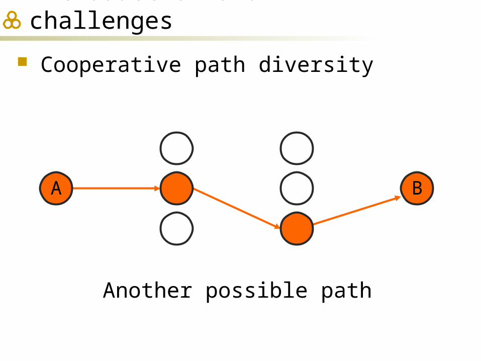
Cooperative path diversity
BA
Another possible path
Introduction and challenges

Cooperative path diversity
B
Many possible paths
A
Introduction and challenges

Cooperative path diversity
B
Best path
A
Introduction and challenges
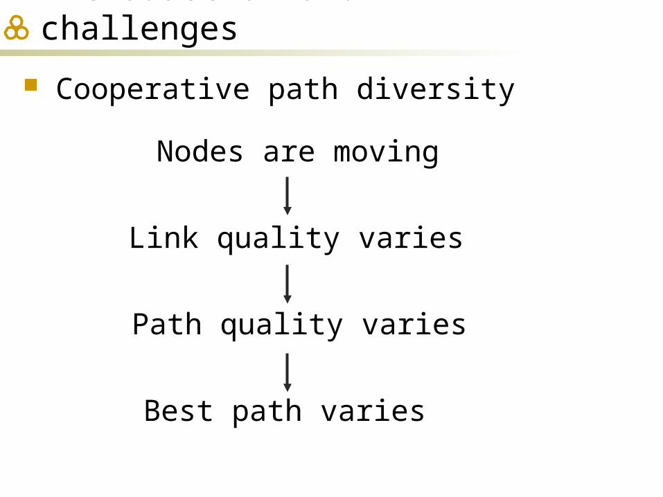
Cooperative path diversity
Nodes are moving
Link quality varies
Best path varies
Path quality varies
Introduction and challenges

Introduction and challenges
Challenges How to define the path quality
based on channel conditions? How to monitor the time-varying
path quality to determine the best path cooperatively?
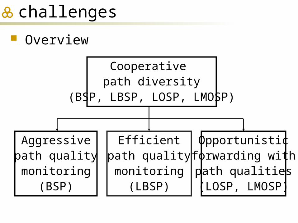
Overview
Cooperative path diversity
(BSP, LBSP, LOSP, LMOSP)
Aggressivepath qualitymonitoring
(BSP)
Efficientpath qualitymonitoring
(LBSP)
Introduction and challenges
Opportunisticforwarding with
path qualities(LOSP, LMOSP)

Introduction and challenges Aggressive path quality monitoring
BSP Efficient path quality monitoring
LBSP Opportunistic forwarding
LBSP2, LOSP, LMOSP Conclusion and future work
Outline
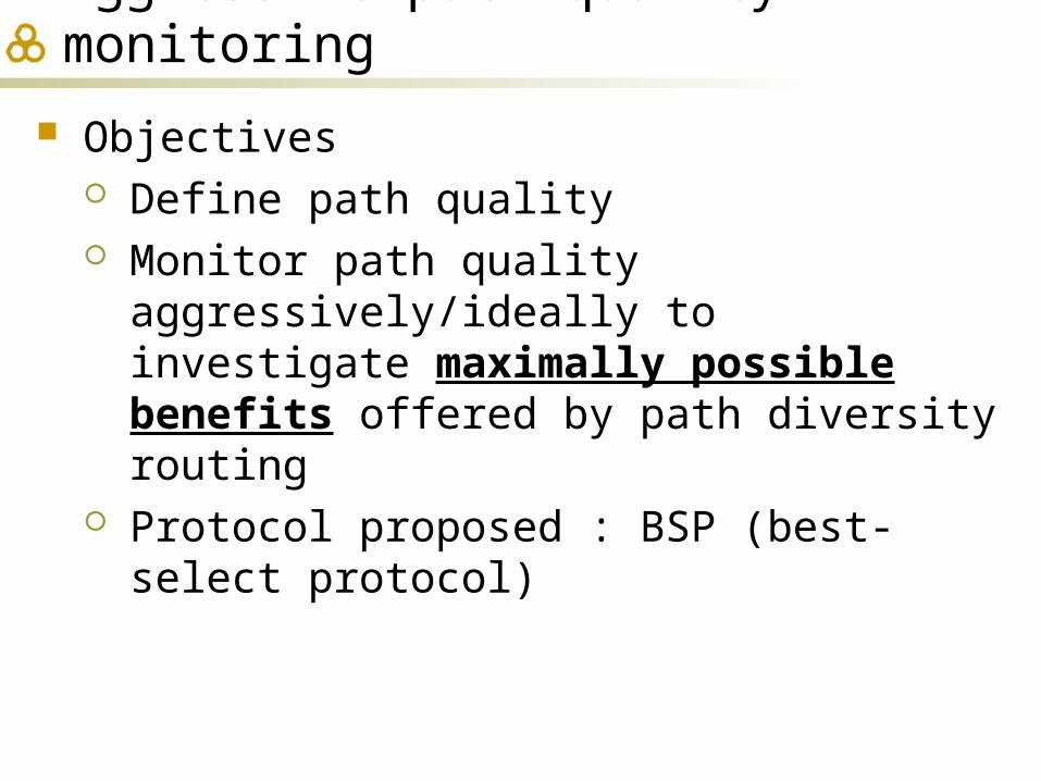
Aggressive path quality monitoring
Objectives Define path quality Monitor path quality aggressively/ideally to
investigate maximally possible benefits offered by path diversity routing
Protocol proposed : BSP (best-select protocol)

Path quality Depends on channel conditions
(e.g., channel loss, SNR, transmit power)
Aggressive path quality monitoring
Depends on protocol designer’s routing objectives Maximize the minimum SNR along the path
(max-min SNR) Maximize delivery probability Maximize throughput Minimize end-to-end delay Minimize total power Minimize total energy
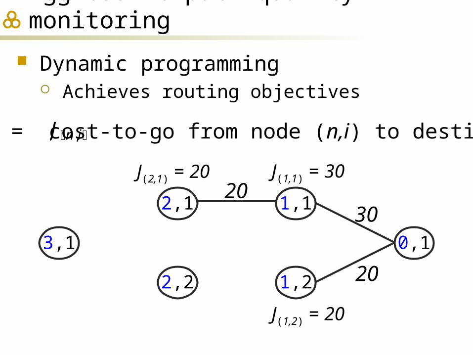
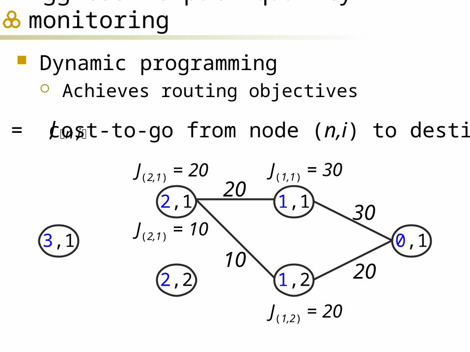
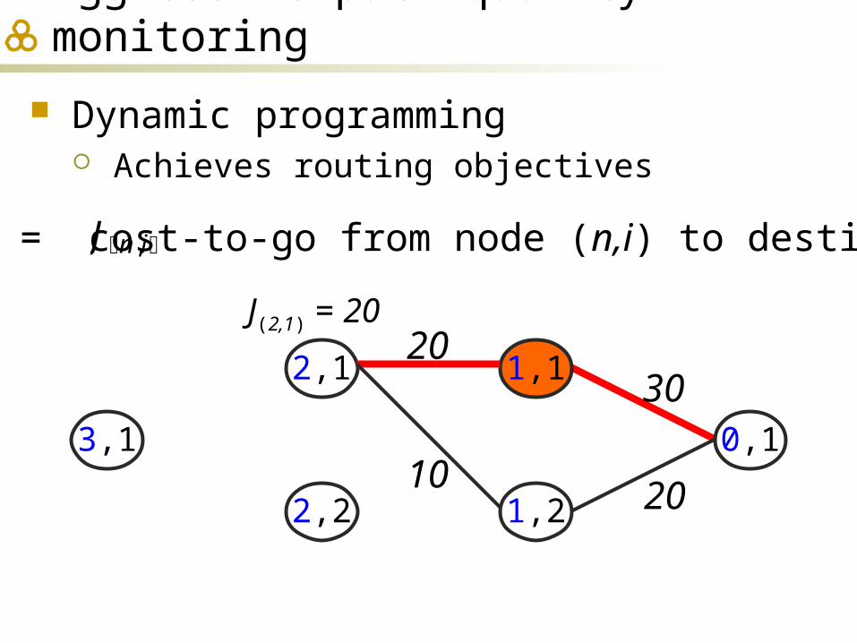
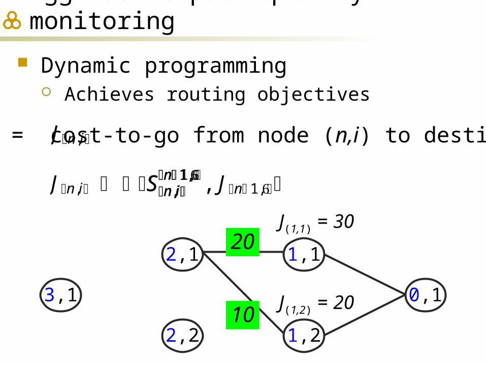
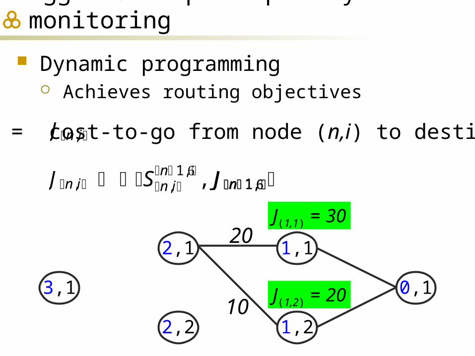
Dynamic programming Achieves routing objectives
Jn,i = cost-to-go from node (n,i) to destination
Aggressive path quality monitoring
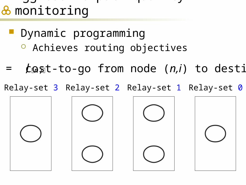
Dynamic programming Achieves routing objectives
Jn,i = cost-to-go from node (n,i) to destination
Relay-set 3 Relay-set 2 Relay-set 1 Relay-set 0
Aggressive path quality monitoring
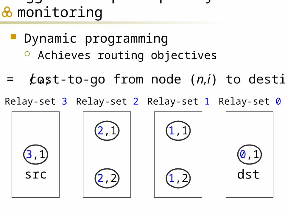
Dynamic programming Achieves routing objectives
0,1
1,1
1,2
2,1
2,2
3,1
Relay-set 3 Relay-set 2 Relay-set 1 Relay-set 0
src dst
Jn,i = cost-to-go from node (n,i) to destination
Aggressive path quality monitoring

Dynamic programming Achieves routing objectives
src dst
0,1
1,1
1,2
2,1
2,2
3,1
Jn,i = cost-to-go from node (n,i) to destination
Aggressive path quality monitoring
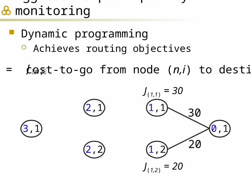
Dynamic programming Achieves routing objectives
0,1
1,1
1,2
2,1
2,2
3,1
Jn,i = cost-to-go from node (n,i) to destination
30
20
J(1,1) = 30
J(1,2) = 20
Aggressive path quality monitoring
Dynamic programming Achieves routing objectives
0,1
1,1
1,2
2,1
2,2
3,1
Jn,i = cost-to-go from node (n,i) to destination
30
20
J(1,1) = 30
J(1,2) = 20
J(2,1) = 2020
Aggressive path quality monitoring
Dynamic programming Achieves routing objectives
0,1
1,1
1,2
2,1
2,2
3,1
Jn,i = cost-to-go from node (n,i) to destination
30
20
J(1,1) = 30
J(1,2) = 20
J(2,1) = 20
10
J(2,1) = 10
20
Aggressive path quality monitoring

Dynamic programming Achieves routing objectives
0,1
1,1
1,2
2,1
2,2
3,1
Jn,i = cost-to-go from node (n,i) to destination
30
20
J(2,1) = 20
10
20
Aggressive path quality monitoring
Dynamic programming Achieves routing objectives
0,1
1,1
1,2
2,1
2,2
3,1
Jn,i = cost-to-go from node (n,i) to destination
30
20
J(2,1) = 20
10
20
Aggressive path quality monitoring

Dynamic programming Achieves routing objectives
0,1
1,1
1,2
2,1
2,2
3,1
Jn,i = cost-to-go from node (n,i) to destination
Aggressive path quality monitoring
Dynamic programming Achieves routing objectives
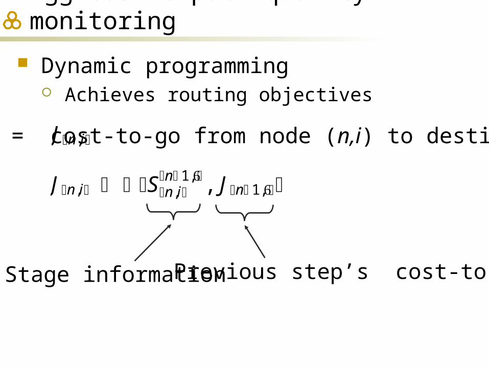
Jn,i = cost-to-go from node (n,i) to destination
Jn,i Sn,in 1,, Jn 1,
Previous step’s cost-to-goStage information
Aggressive path quality monitoring
Dynamic programming Achieves routing objectives
Jn,i = cost-to-go from node (n,i) to destination
Jn,i Sn,in 1,, Jn 1,
0,1
1,1
1,2
2,1
2,2
3,1
J(1,1) = 30
J(1,2) = 2010
20
Sn,in 1,
Aggressive path quality monitoring
Dynamic programming Achieves routing objectives
Jn,i = cost-to-go from node (n,i) to destination
Jn,i Sn,in 1,, Jn 1,
0,1
1,1
1,2
2,1
2,2
3,1
J(1,1) = 30
J(1,2) = 2010
20
Jn 1,
Aggressive path quality monitoring
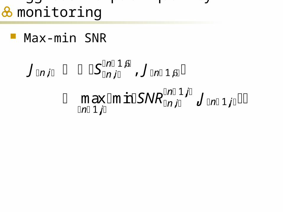
Max-min SNR
Jn,i Sn,in 1,, Jn 1,
maxn 1,j
minSNRn,in 1,j
, Jn 1,j
Aggressive path quality monitoring
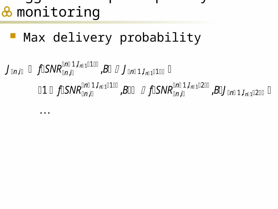
Max delivery probability
Jn,i fSNRn,in 1,In11 , B Jn 1,In11
1 fSNRn,in 1,In11 , B fSNRn,i
n 1,In12 , BJn 1,In12
. . .
Aggressive path quality monitoring

Max delivery probability
Jn,i fSNRn,in 1,In11 , B Jn 1,In11
1 fSNRn,in 1,In11 , B fSNRn,i
n 1,In12 , BJn 1,In12
. . .
Aggressive path quality monitoring
Jn 1,1 0. 8
Jn 1,2 0. 9
Jn 1,3 0. 7
In 11 2
In 12 1
In 13 3
Max delivery probability
Jn,i fSNRn,in 1,In11 , B Jn 1,In11
1 fSNRn,in 1,In11 , B fSNRn,i
n 1,In12 , BJn 1,In12
. . .
Aggressive path quality monitoring
n,i
n-1,In-1(1)
n-1,In-1(2)
n-1,In-1(3)

Max delivery probability
Jn,i fSNRn,in 1,In11 , B Jn 1,In11
1 fSNRn,in 1,In11 , B fSNRn,i
n 1,In12 , BJn 1,In12
. . .
Aggressive path quality monitoring
n,i
n-1,In-1(1)
n-1,In-1(2)
n-1,In-1(3)
Max delivery probability
Jn,i fSNRn,in 1,In11 , B Jn 1,In11
1 fSNRn,in 1,In11 , B fSNRn,i
n 1,In12 , BJn 1,In12
. . .
Aggressive path quality monitoring
n-1,In-1(1)
n-1,In-1(2)
n-1,In-1(3)
n,i
Max throughput
Jn,i maxjmaxB|fSNR n,in1,j
,B PROB_THRESH minB, Jn 1,j
Aggressive path quality monitoring

Min end-to-end delay
Jn,i minB Jn,iB
Aggressive path quality monitoring
Jn,iB packet sizeB
Psucc Dn 1 T P fail
Psucc fSNRn,in 1,In11 , B
1 fSNRn,in 1,In11 , BfSNRn,i
n 1,In12 , B
Dn 1 fSNRn,in 1,In11 , BJn 1,In11
1 fSNRn,in 1,In11 , BfSNRn,i
n 1,In12 , BJn 1,In12
P fail 1 fSNRn,in 1,In11 , B1 fSNRn,i
n 1,In12 , B
#
Min total power
Jn,i minn 1,j 10SNR_THRESH Hn,i
n1,jN
10 Jn 1,j
Aggressive path quality monitoring
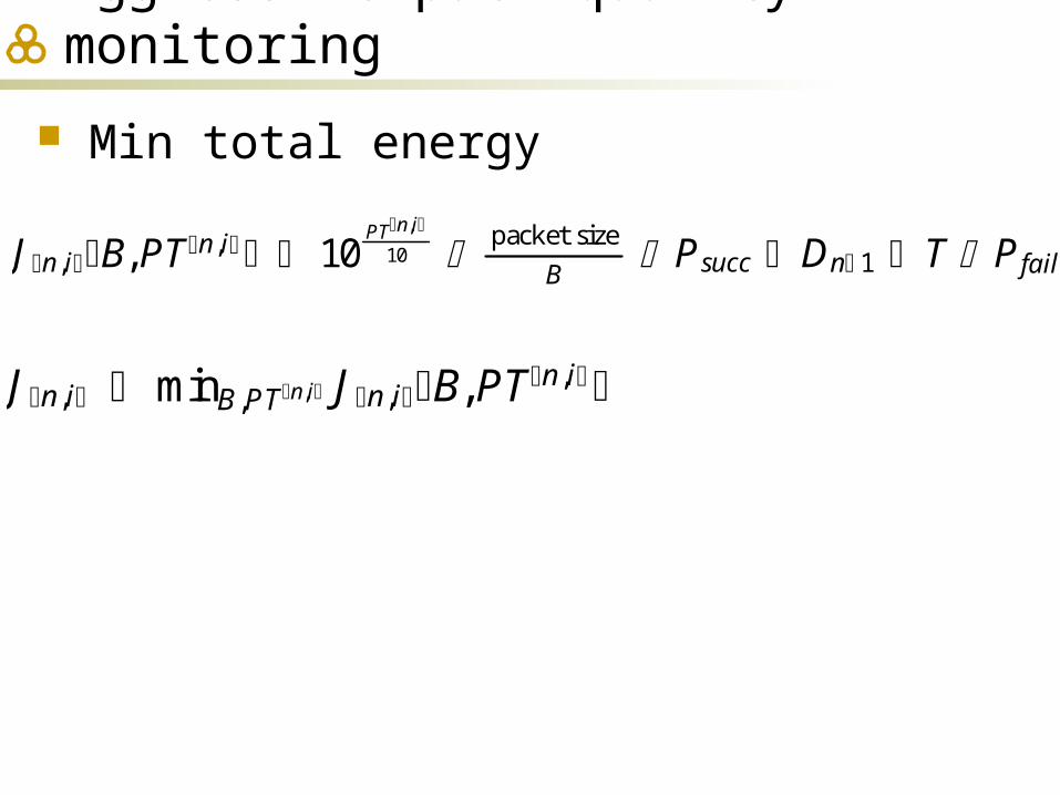
Min total energy
Jn,iB, PTn,i 10PTn,i
10 packet size
B Psucc Dn 1 T P fail
Aggressive path quality monitoring
Jn,i minB,PTn,i Jn,iB, PTn,i

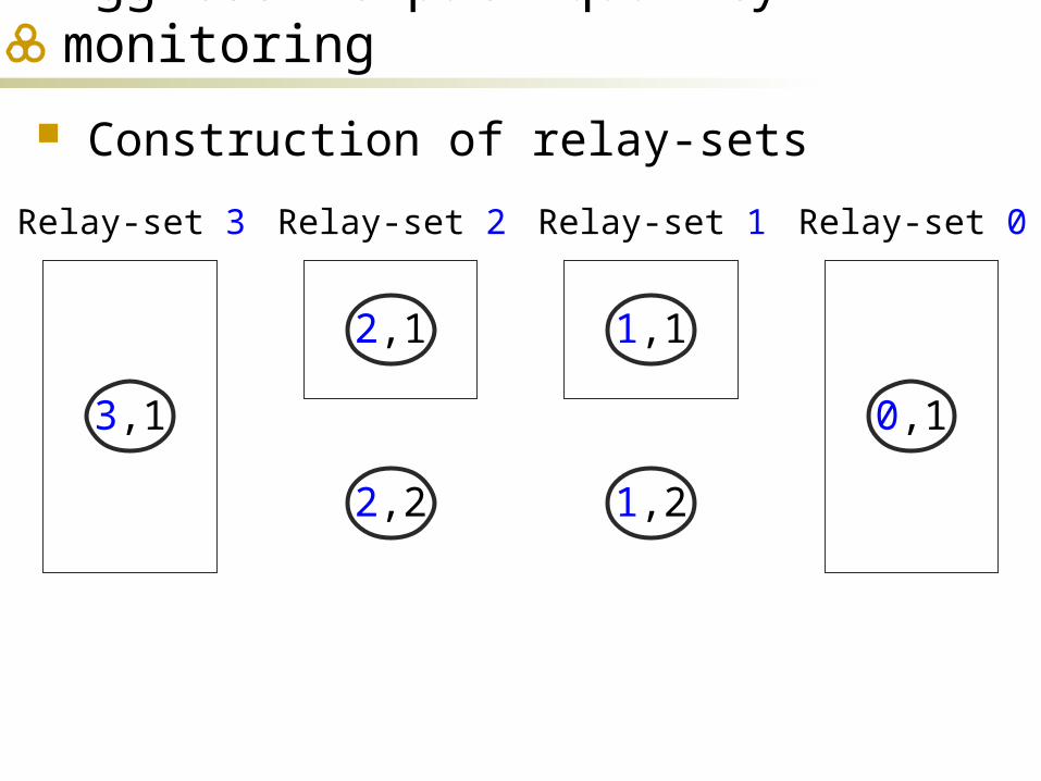
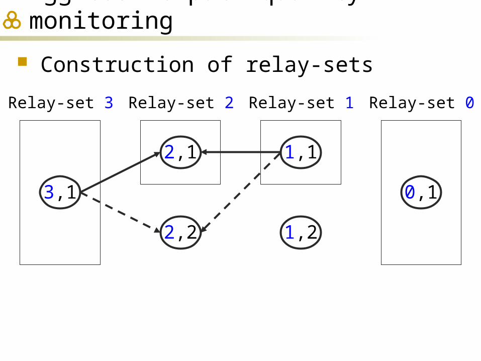
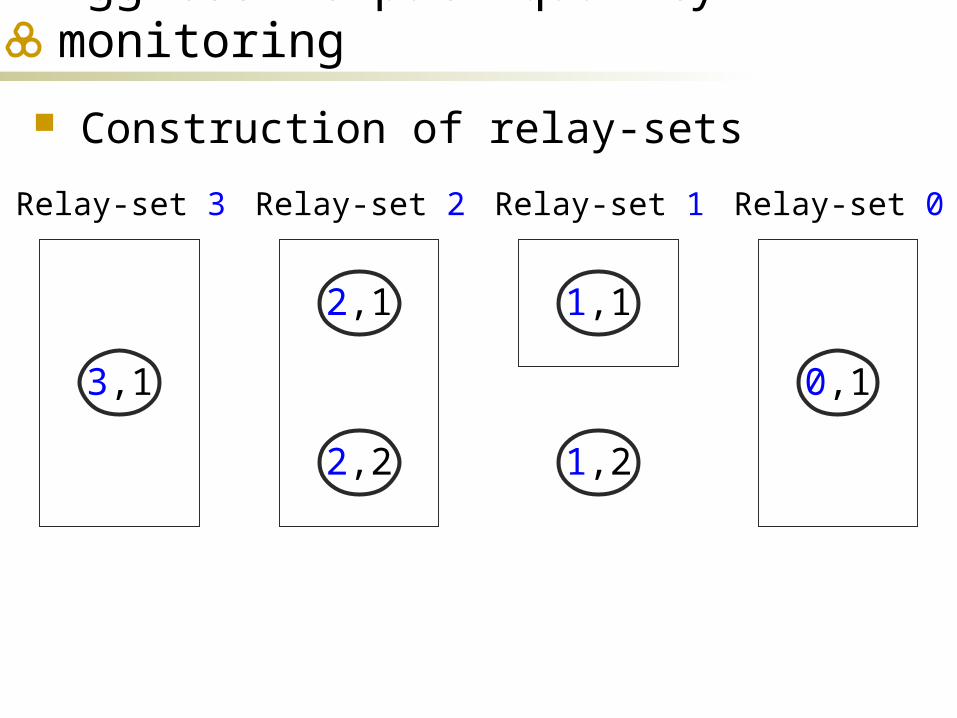
Construction of relay-sets
0,1
1,1
1,2
2,1
2,2
3,1
AODV finds a traditional single path
Aggressive path quality monitoring
Construction of relay-sets
0,1
1,1
1,2
2,1
2,2
3,1
Relay-set 3 Relay-set 2 Relay-set 1 Relay-set 0
Aggressive path quality monitoring
Construction of relay-sets
0,1
1,1
1,2
2,1
2,2
3,1
Relay-set 3 Relay-set 2 Relay-set 1 Relay-set 0
Aggressive path quality monitoring
Construction of relay-sets
0,1
1,1
1,2
2,1
2,2
3,1
Relay-set 3 Relay-set 2 Relay-set 1 Relay-set 0
Aggressive path quality monitoring

Construction of relay-sets
0,1
1,1
1,2
2,1
2,2
3,1
Relay-set 3 Relay-set 2 Relay-set 1 Relay-set 0
Aggressive path quality monitoring

Path quality monitoring
0,1
1,1
1,2
2,1
2,2
3,1
CIEREQ (channel info exchange request)CIEREP (channel info exchange reply)
Relay-set 3 Relay-set 2 Relay-set 1 Relay-set 0
Aggressive path quality monitoring

Path quality monitoring
0,1
1,1
1,2
2,1
2,2
3,1
CIEREQ
CIEREQ
: data frame
Aggressive path quality monitoring
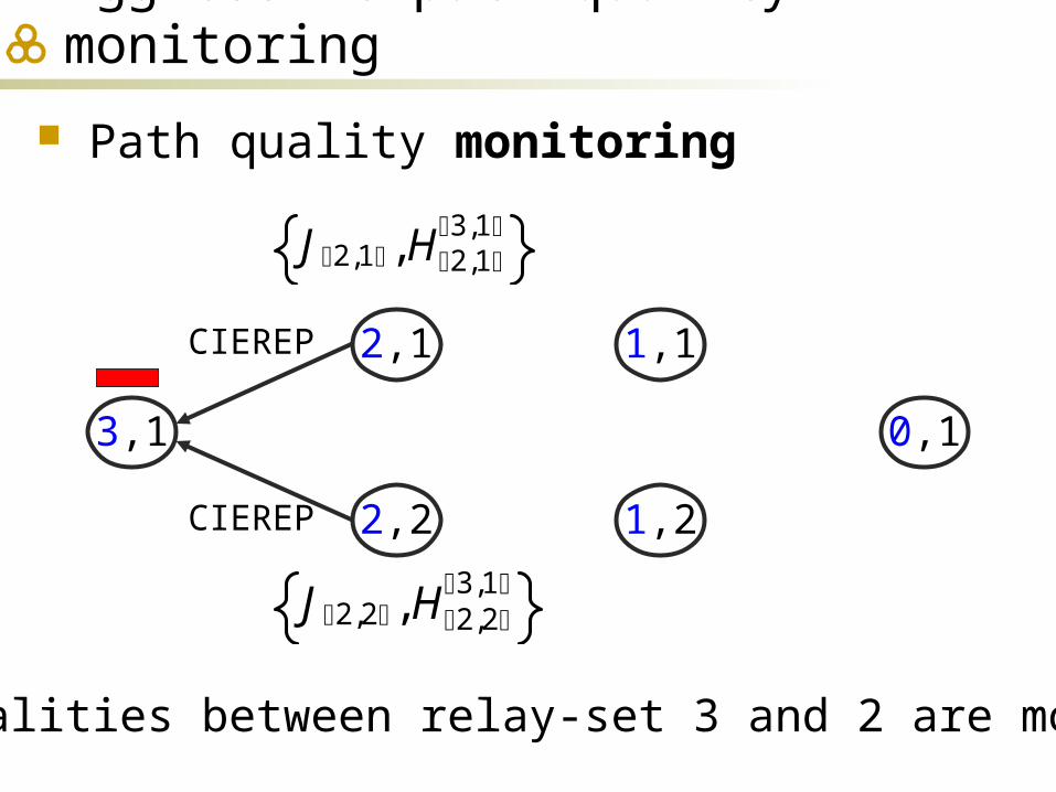
Path quality monitoring
0,1
1,1
1,2
2,1
2,2
3,1
CIEREP
CIEREP
J2,1 , H2,1 3,1
J2,2 , H2,2 3,1
Path qualities between relay-set 3 and 2 are monitored
Aggressive path quality monitoring
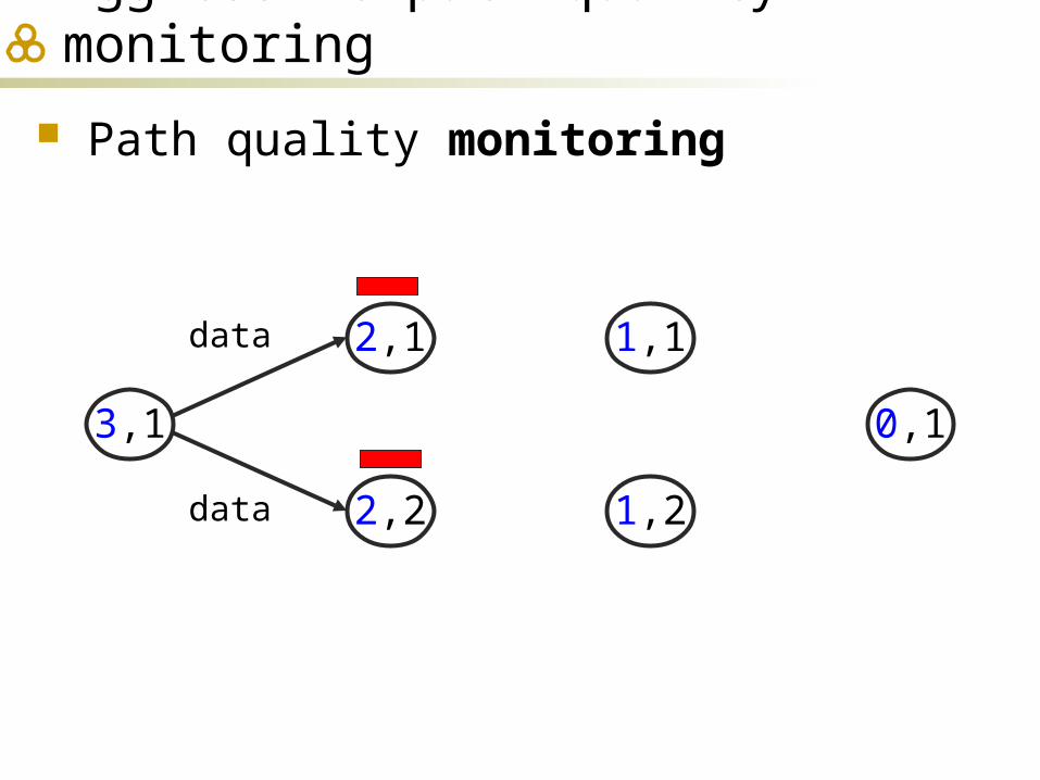
Path quality monitoring
0,1
1,1
1,2
2,1
2,2
3,1
data
data
Aggressive path quality monitoring
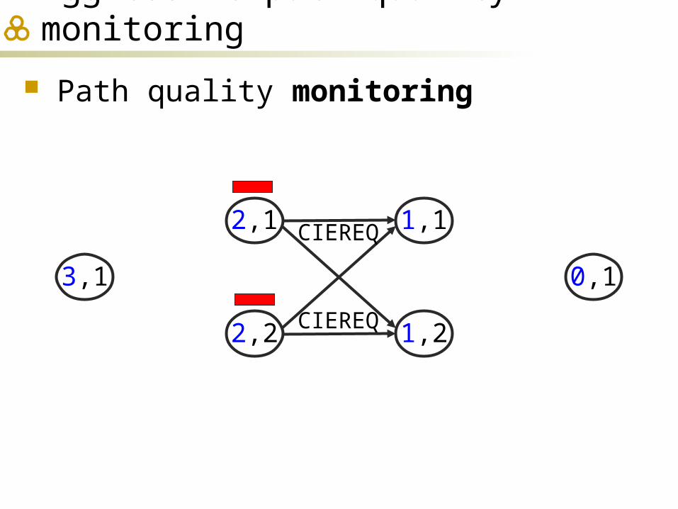
Path quality monitoring
0,1
1,1
1,2
2,1
2,2
3,1
CIEREQ
CIEREQ
Aggressive path quality monitoring

Path quality monitoring
0,1
1,1
1,2
2,1
2,2
3,1
CIEREP
CIEREP
J1,1 , H1,1 2,1 , H1,1
2,2
J1,2 , H1,2 2,1 , H1,2
2,2
Path qualities between relay-set 2 and 1 are monitored
Aggressive path quality monitoring

Path quality monitoring
0,1
1,1
1,2
2,1
2,2
3,1
J2,1 J1,1 , J1,2 , H1,1 2,1 , H1,2
2,1
J2,2 J1,1 , J1,2 , H1,1 2,2 , H1,2
2,2 J2,1 J2,2
Assume that
Aggressive path quality monitoring
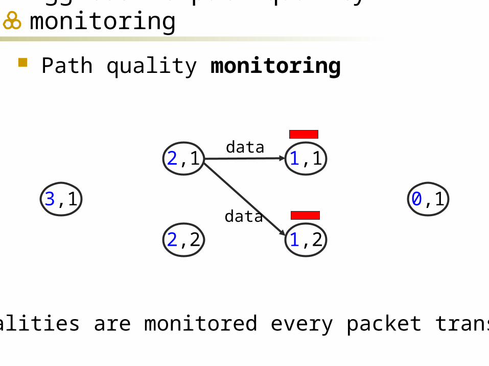
Path quality monitoring
0,1
1,1
1,2
2,1
2,2
3,1
data
data
Path qualities are monitored every packet transmission
Aggressive path quality monitoring
Path quality monitoring
0,1
1,1
1,2
2,1
2,2
3,1
Aggressive path quality monitoring

Simulation UDelModels :
Urban city, mobility, channel models Numerical analysis
Ideally construct relay-sets and receive CIEREQ/CIEREP Packet level simulation
QualNet network simulator CBR traffic (1024 bytes per second)
Comparison between J
single and J diversity
J single : source’s J along the single path found initially J diversity : source’s J along the best path among all paths
Aggressive path quality monitoring

Results : benefits of path diversity
Aggressive path quality monitoring
2 4 6 8 100
5
10
15
20
25
30 SparseDense
2
4
6
8
10
2 4 6 8 100
SparseDense
2 4 6 8 100
5
10
15SparseDense
2 4 6 8 100
5
10
15 SparseDense
2 4 6 8 10100
101
102
103
104
SparseDense
2 4 6 8 10100
101
102
103
SparseDense
Max delivery prob. Max throughput
J di
vers
ity /
J si
ngle
Max-min SNR
J di
vers
ity —
J si
ngle
J di
vers
ity /
J si
ngle
Min power Min energyMin delay
J di
vers
ity /
J si
ngle
J di
vers
ity /
J si
ngle
J di
vers
ity /
J si
ngle

Results : path selection differences
Aggressive path quality monitoring
2 4 6 8 100
0.2
0.4
0.6
0.8
1
Fra
ctio
n o
f re
lays
sh
ared
Minimum relay-set size
max-min SNRmax throughput
min total power min energy
min end-to-end delay max delivery probability
vs.
vs.vs.

Introduction and challenges Aggressive path quality monitoring
BSP Efficient path quality monitoring
LBSP Opportunistic forwarding
LBSP2, LOSP, LMOSP Conclusion and future work
Outline

Efficient path quality monitoring
Objectives Monitor path quality efficiently to
reduce overhead J broadcast, J-test, power control
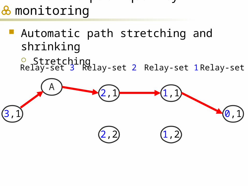
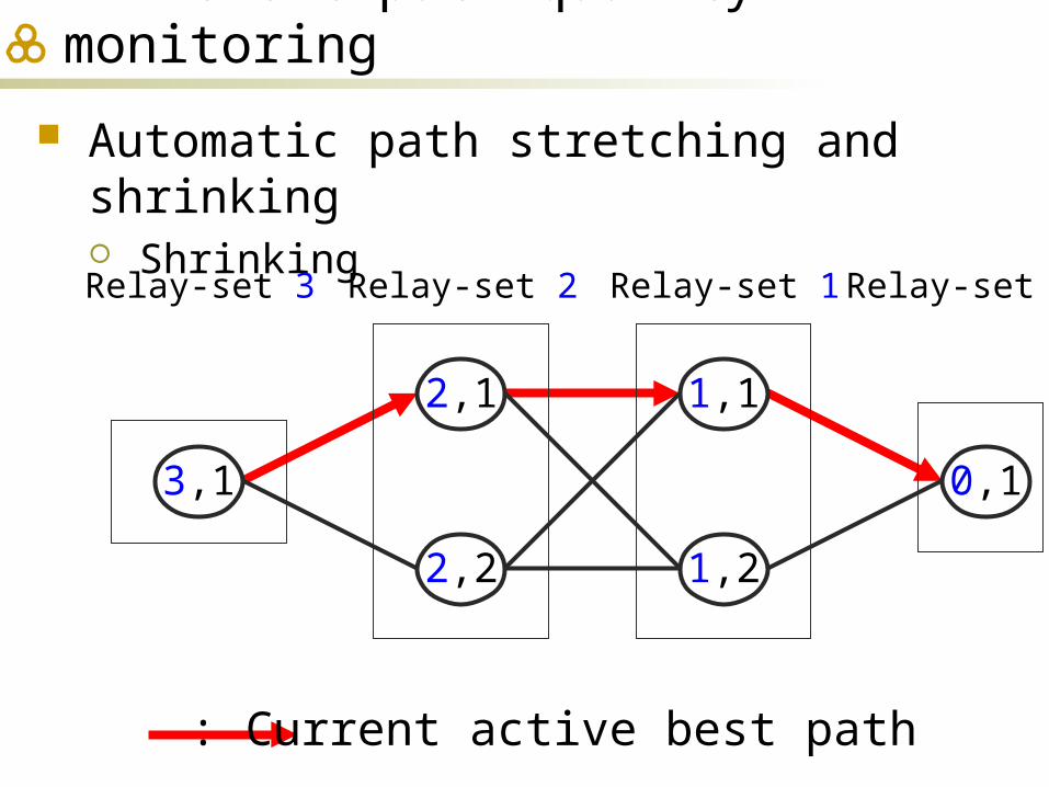
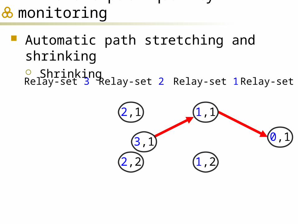
Robust routing function Automatic path stretching and shrinking
Protocol proposed : LBSP (local BSP)
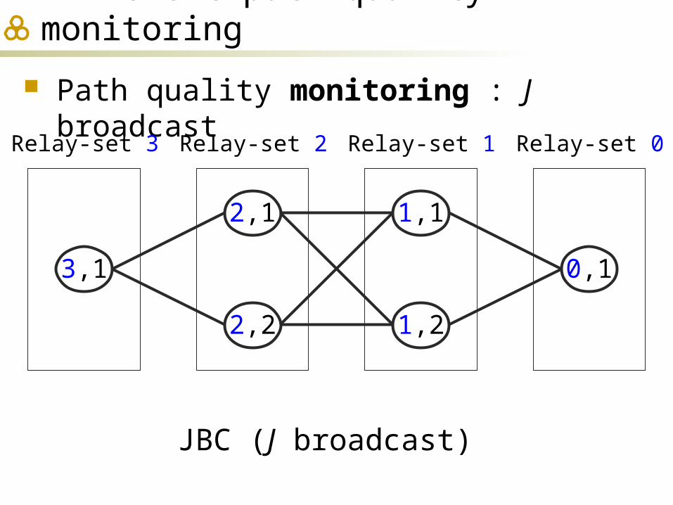
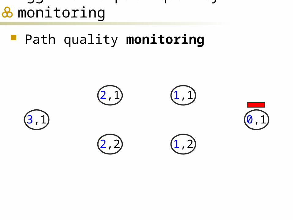
Path quality monitoring : J broadcast
0,1
1,1
1,2
2,1
2,2
3,1
JBC (J broadcast)
Relay-set 3 Relay-set 2 Relay-set 1 Relay-set 0
Efficient path quality monitoring

Path quality monitoring : J broadcast
0,1
1,1
1,2
2,1
2,2
3,1
Efficient path quality monitoring
J0,10,1
Path quality monitoring : J broadcast
0,1
1,1
1,2
2,1
2,2
3,1
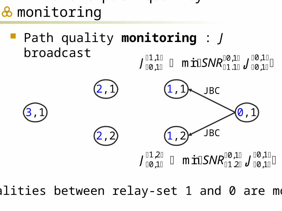
Efficient path quality monitoring
JBC
JBC
J0,11,1 minSNR1.1
0,1, J0,10,1
J0,11,2 minSNR1.2
0,1, J0,10,1
Path qualities between relay-set 1 and 0 are monitored
Path quality monitoring : J broadcast
0,1
1,1
1,2
2,1
2,2
3,1
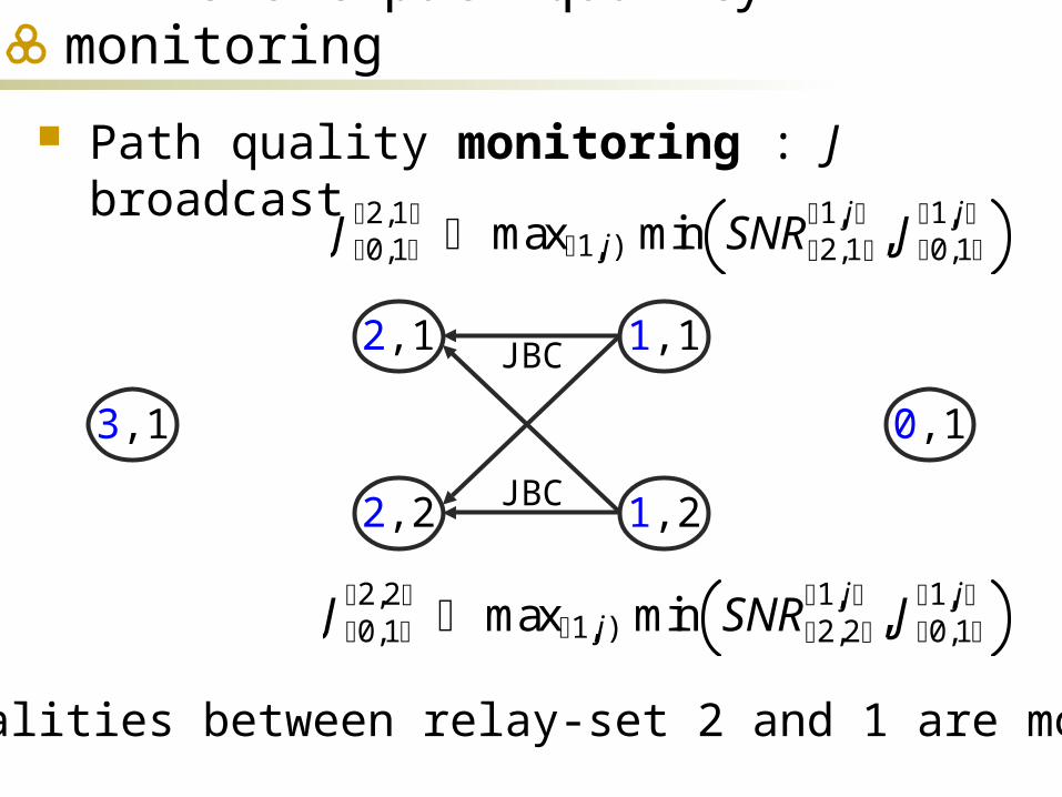
Efficient path quality monitoring
JBC
JBC
J0,12,1 max1,j) min SNR2,1
1,j, J0,1
1,j
J0,12,2 max1,j) min SNR2,2
1,j, J0,1
1,j
Path qualities between relay-set 2 and 1 are monitored

Path quality monitoring : J broadcast
0,1
1,1
1,2
2,1
2,2
3,1
Efficient path quality monitoring
JBC
JBC
J0,13,1 max2,j) min SNR3,1
2,j, J0,1
2,j
Path qualities between relay-set 3 and 2 are monitored

Path quality monitoring : J broadcast
0,1
1,1
1,2
2,1
2,2
3,1
Efficient path quality monitoring
: best path
Next hop best node
arg maxn 1,j) min SNRn,1 n 1,j, J0,1
n 1,j

Path quality monitoring : J broadcast When this J-broadcast occurs?
When current best path quality degradation is experienced.
Efficient path quality monitoring
Jsrcdst Jsrc
dst Jthreshold or Jsrcdst Jmin
0,1
1,22,2
3,1
src dst
Jsrcsrc
Jsrc2,2 Jsrc
1,2Jsrc
dst

Path quality monitoring : J broadcast When this J-broadcast occurs?
When current best path quality degradation is experienced.
Efficient path quality monitoring
Jsrcdst Jsrc
dst Jthreshold or Jsrcdst Jmin
Reference path quality for the first data frame
Path quality for the subsequent data frame
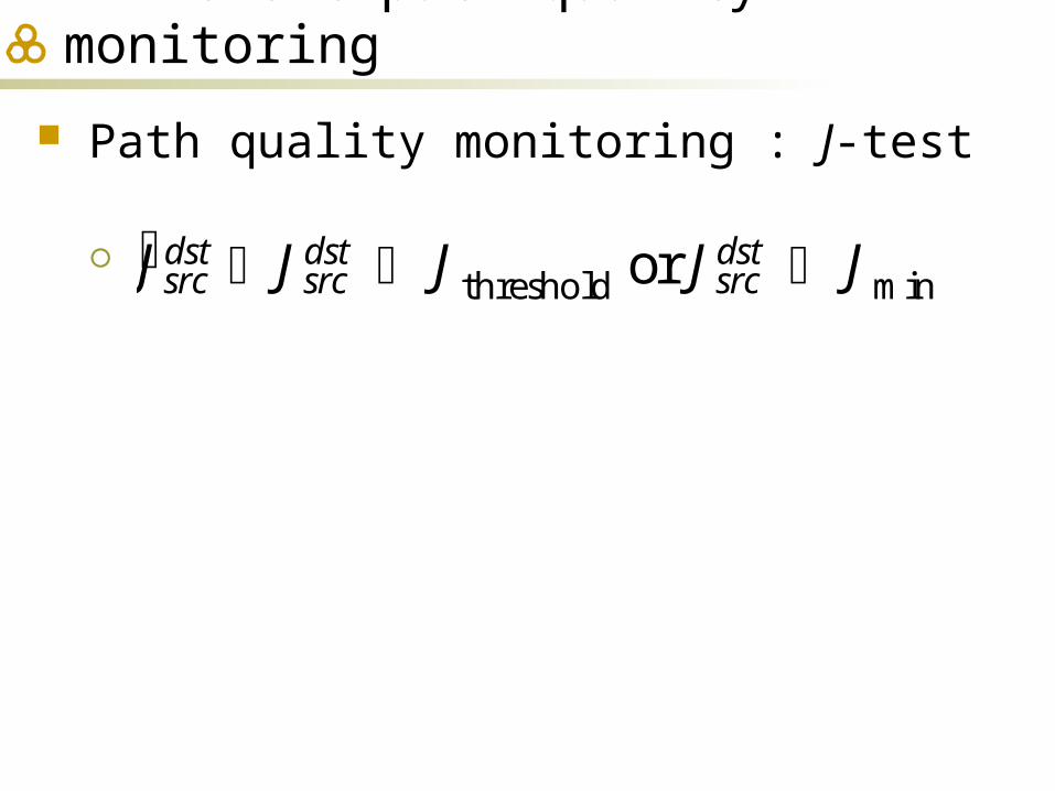
Efficient path quality monitoring
Path quality monitoring : J-test
Jsrcdst Jsrc
dst Jthreshold or Jsrcdst Jmin
n-1,1
n-1,3
n-1,2
JBC
n,iJBCJBC
Jdstn,i maxn 1,j min SNRn,i
n 1,j, Jdst
n 1,j
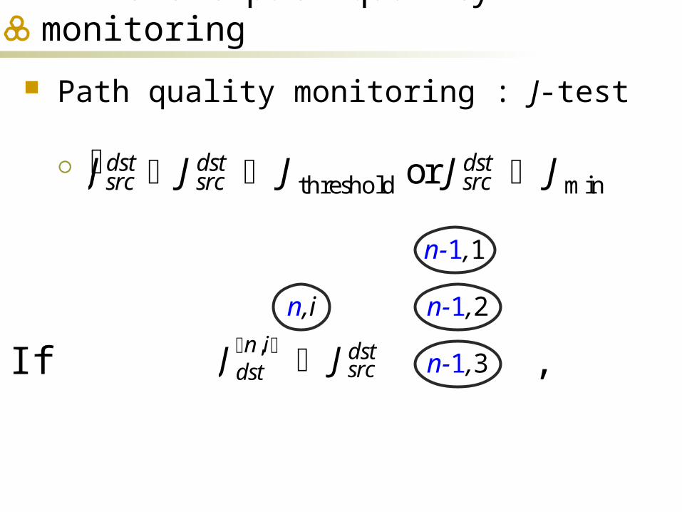
Efficient path quality monitoring
Path quality monitoring : J-test
Jsrcdst Jsrc
dst Jthreshold or Jsrcdst Jmin
n-1,1
n-1,3
n-1,2n,i
Jdstn,i Jsrc
dstIf ,
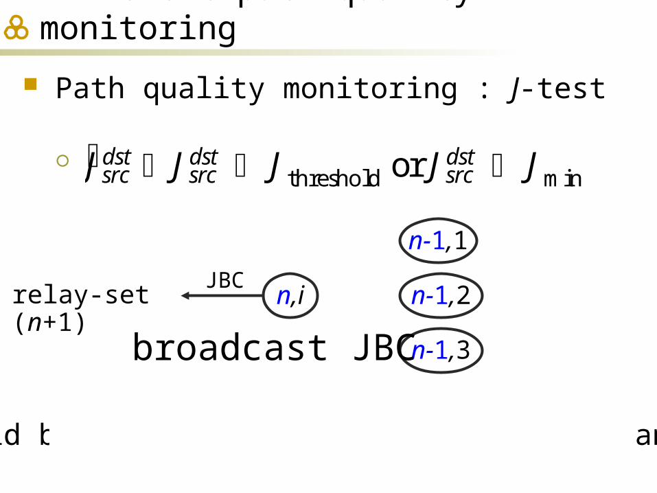
Efficient path quality monitoring
Path quality monitoring : J-test
Jsrcdst Jsrc
dst Jthreshold or Jsrcdst Jmin
n-1,1
n-1,3
n-1,2
broadcast JBC
JBCrelay-set (n+1)
Avoid broadcasting lower path quality than Jsrcdst
n,i

Efficient path quality monitoring
Path quality monitoring : power control
Efficient path quality advertisement
Higher path qualityLower path quality
Higher powerLower power
n,1
n,3
n,2n+1,i
PRn 1,in,1 PRn 1,i
n,2 PRn 1,in,3
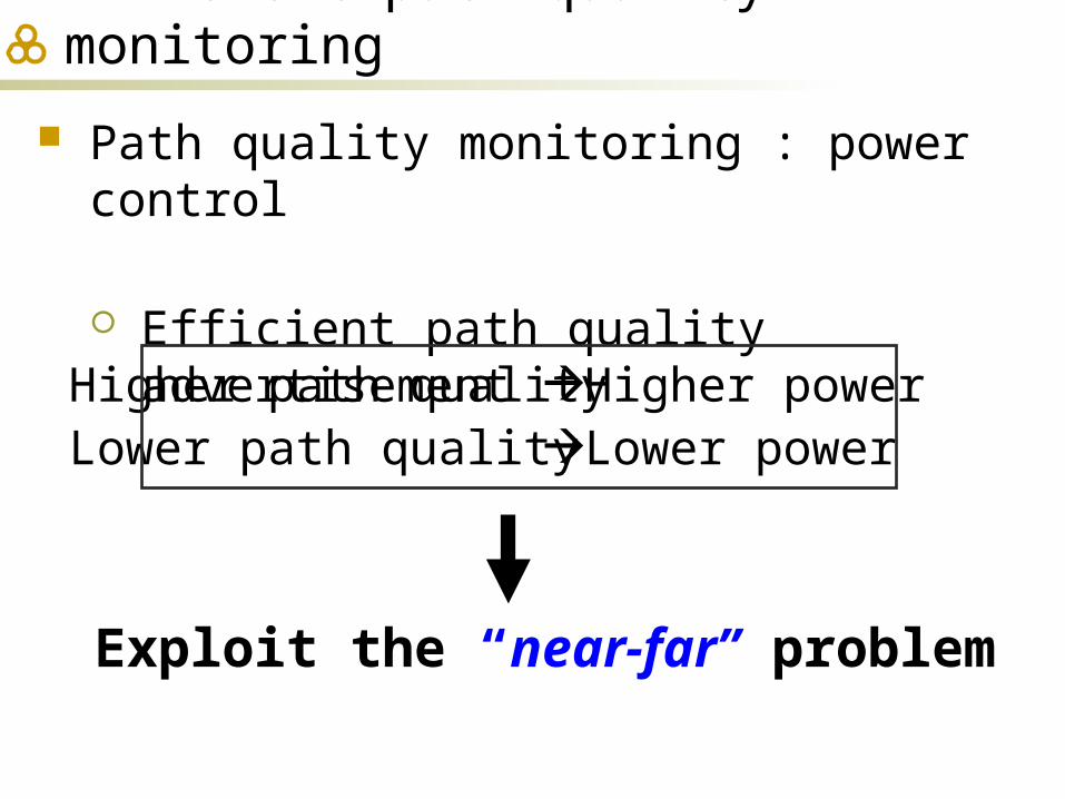
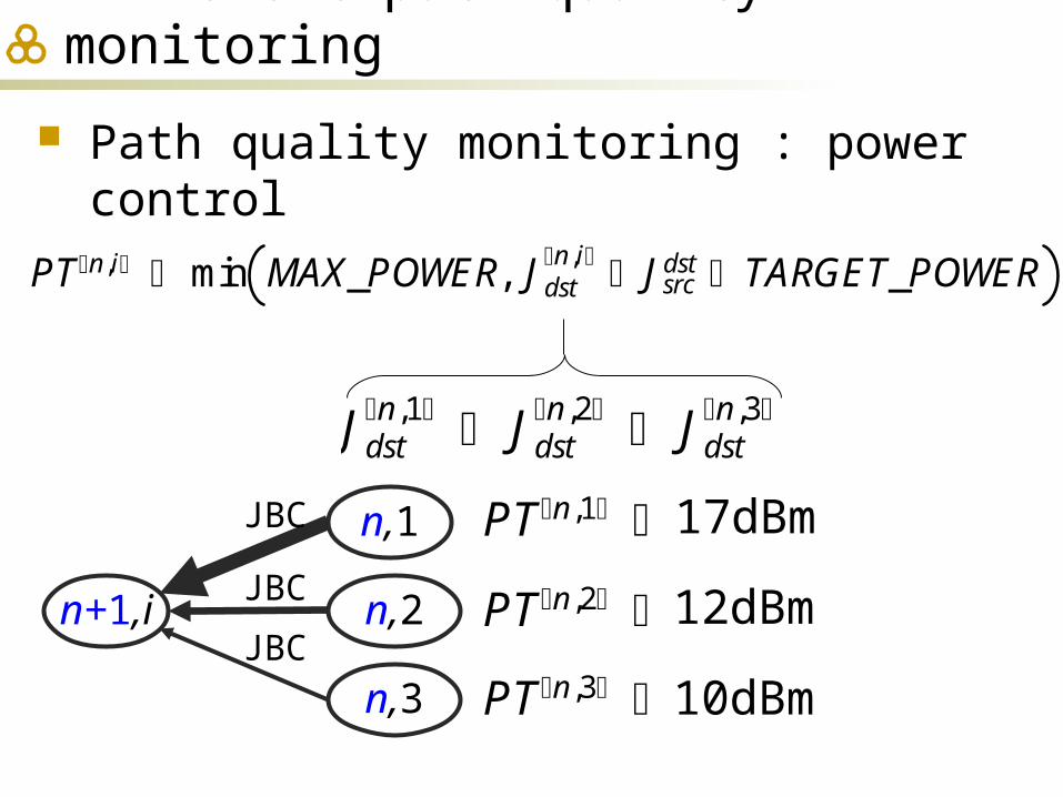
Efficient path quality monitoring
Path quality monitoring : power control
Efficient path quality advertisement
Higher path qualityLower path quality
Higher powerLower power
Exploit the “near-far” problem

Efficient path quality monitoring
Path quality monitoring : power control
PTn,i min MAX_POWER, Jdstn,i Jsrc
dst TARGET_POWER
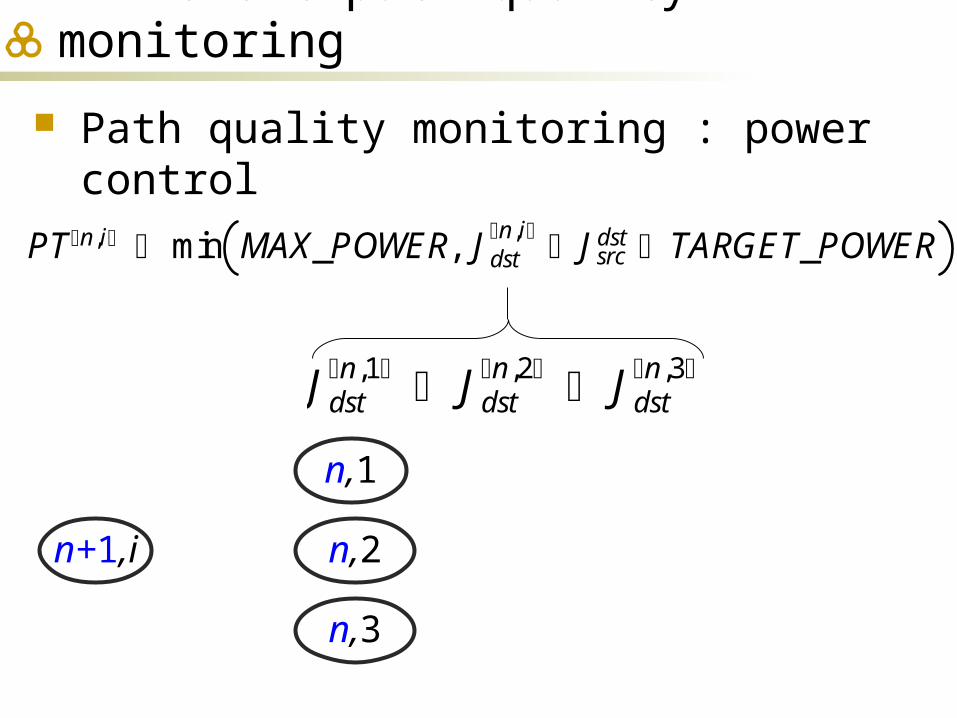
Efficient path quality monitoring
Path quality monitoring : power control
PTn,i min MAX_POWER, Jdstn,i Jsrc
dst TARGET_POWER
n,1
n,3
n,2n+1,i
PTn,1
PTn,2
PTn,3
17dBm
12dBm
10dBm
Jdstn,1 Jdst
n,2 Jdstn,3
Efficient path quality monitoring
Path quality monitoring : power control
PTn,i min MAX_POWER, Jdstn,i Jsrc
dst TARGET_POWER
n,1
n,3
n,2n+1,i
PTn,1
PTn,2
PTn,3
17dBm
12dBm
10dBm
Jdstn,1 Jdst
n,2 Jdstn,3
JBC
JBC
JBC
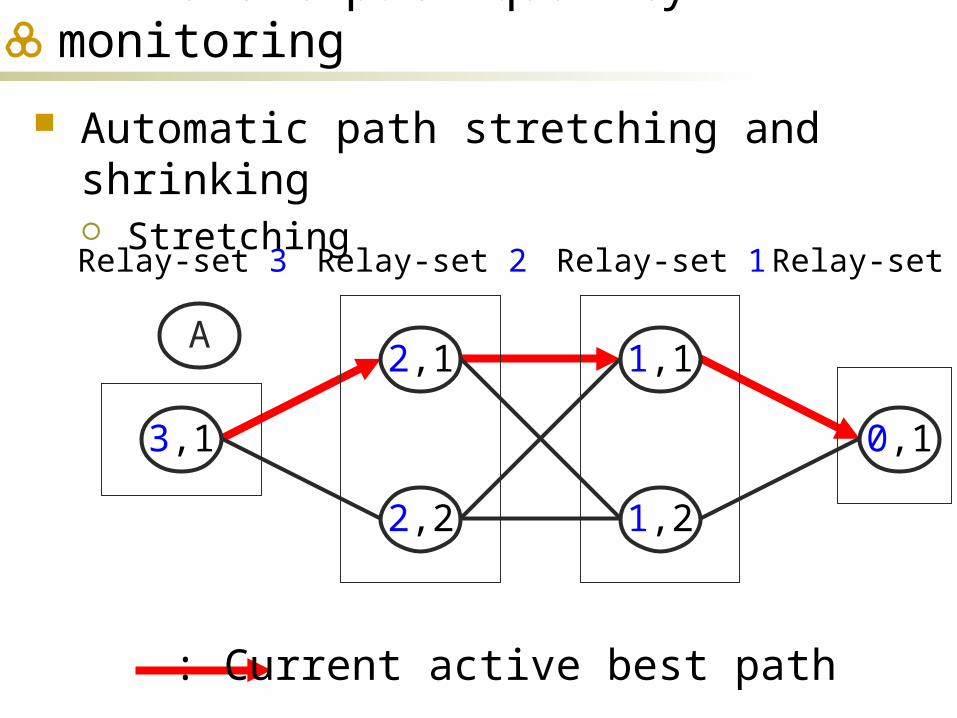
Efficient path quality monitoring
Automatic path stretching and shrinking Stretching
0,1
1,1
1,2
2,1
2,2
3,1
Relay-set 3 Relay-set 2 Relay-set 1 Relay-set 0
A
: Current active best path
Efficient path quality monitoring
Automatic path stretching and shrinking Stretching
0,1
1,1
1,2
2,1
2,2
3,1
Relay-set 3 Relay-set 2 Relay-set 1 Relay-set 0
A
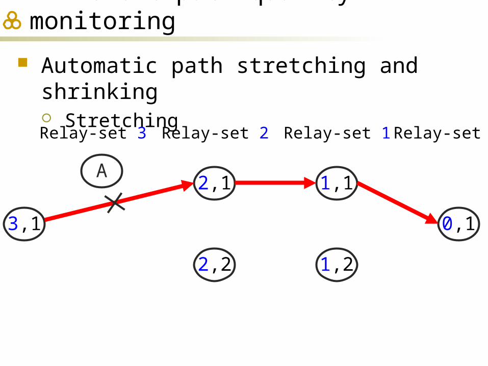
Efficient path quality monitoring
Automatic path stretching and shrinking Stretching
0,1
1,1
1,2
2,1
2,2
3,1
Relay-set 3 Relay-set 2 Relay-set 1 Relay-set 0
A

Efficient path quality monitoring
Automatic path stretching and shrinking Stretching
0,1
1,1
1,2
2,1
2,2
4,1
Relay-set 3 Relay-set 2 Relay-set 1 Relay-set 0
3,1
Relay-set 4
Efficient path quality monitoring
Automatic path stretching and shrinking Shrinking
0,1
1,1
1,2
2,1
2,2
3,1
Relay-set 3 Relay-set 2 Relay-set 1 Relay-set 0
: Current active best path

Efficient path quality monitoring
Automatic path stretching and shrinking Shrinking
0,1
1,1
1,2
2,1
2,2
3,1
Relay-set 3 Relay-set 2 Relay-set 1 Relay-set 0
Efficient path quality monitoring
Automatic path stretching and shrinking Shrinking
0,1
1,1
1,2
2,1
2,2
3,1
Relay-set 3 Relay-set 2 Relay-set 1 Relay-set 0

Efficient path quality monitoring
Automatic path stretching and shrinking Shrinking
0,1
1,1
1,2
2,1
2,2
2,3
Relay-set 3 Relay-set 2 Relay-set 1 Relay-set 0

Efficient path quality monitoring
Numerical analysis : setting
source destination
50m 100m 100m 50m
relay-set 2 relay-set 1relay-set 3 relay-set 0
Efficient path quality monitoring
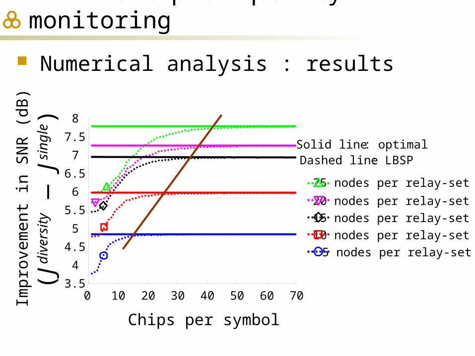
Numerical analysis : results
25 nodes per relay-set
20 nodes per relay-set
15 nodes per relay-set
10 nodes per relay-set
5 nodes per relay-set
0 10 20 30 40 50 60 703.5
4
4.5
5
5.5
6
6.5
7
7.5
8
Solid lineDashed line
: optimal: LBSP
Chips per symbol
Impr
ovem
ent
in S
NR
(dB
)
(J di
vers
ity —
J si
ngle)
Efficient path quality monitoring
Numerical analysis : results
Chips per symbol
Impr
ovem
ent
in S
NR
(dB
)
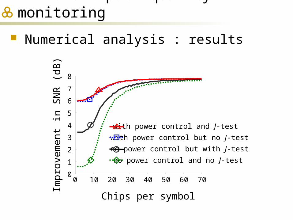
no power control and no J-test
no power control but with J-test
with power control but no J-test
with power control and J-test
0 10 20 30 40 50 60 700
1
2
3
4
5
6
7
8
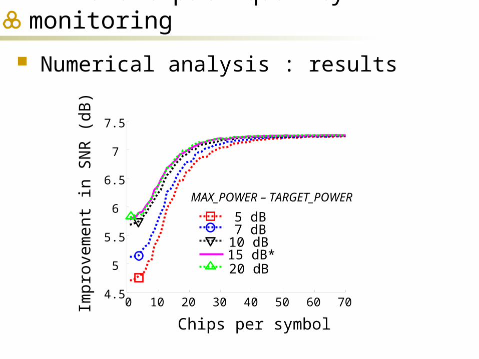
Efficient path quality monitoring
Numerical analysis : results
Chips per symbol
Impr
ovem
ent
in S
NR
(dB
)
0 10 20 30 40 50 60 704.5
5
5.5
6
6.5
7
7.5
MAX_POWER – TARGET_POWER
5 dB7 dB
10 dB15 dB*20 dB
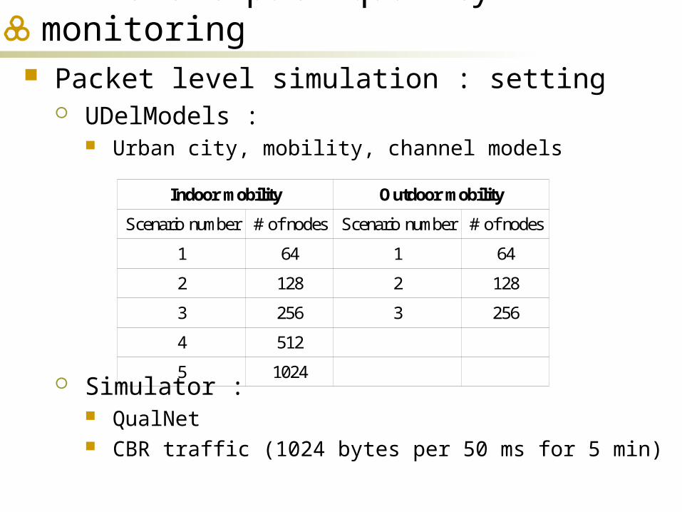
Efficient path quality monitoring Packet level simulation : setting
UDelModels : Urban city, mobility, channel models
Simulator : QualNet CBR traffic (1024 bytes per 50 ms for 5 min)
Indoor mobility Outdoor mobility
Scenario number # of nodes Scenario number # of nodes
1 64 1 64
2 128 2 128
3 256 3 256
4 512
5 1024
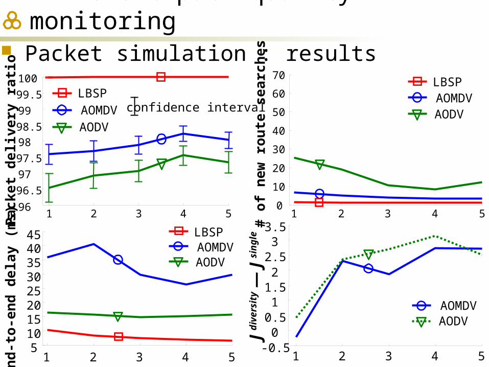
Efficient path quality monitoring Packet simulation : results
Pa
cke
t d
eliv
ery
rat
io
1 2 3 4 596
96.5
97
97.5
98
98.5
99
99.5
100
AODVAOMDVLBSP
confidence interval
# o
f n
ew
ro
ute
sea
rch
es
1 2 3 4 50
10
20
30
40
50
60
70
AODVAOMDVLBSP
En
d-t
o-e
nd
de
lay
(m
s)
1 2 3 4 55
1015202530354045
AODVAOMDVLBSP
J di
vers
ity —
J si
ngl
e
1 2 3 4 5-0.50
0.51
1.52
2.53
3.5
AODVAOMDV

Introduction and challenges Aggressive path quality monitoring
BSP Efficient path quality monitoring
LBSP Opportunistic forwarding
LBSP2, LOSP, LMOSP Conclusion and future work
Outline
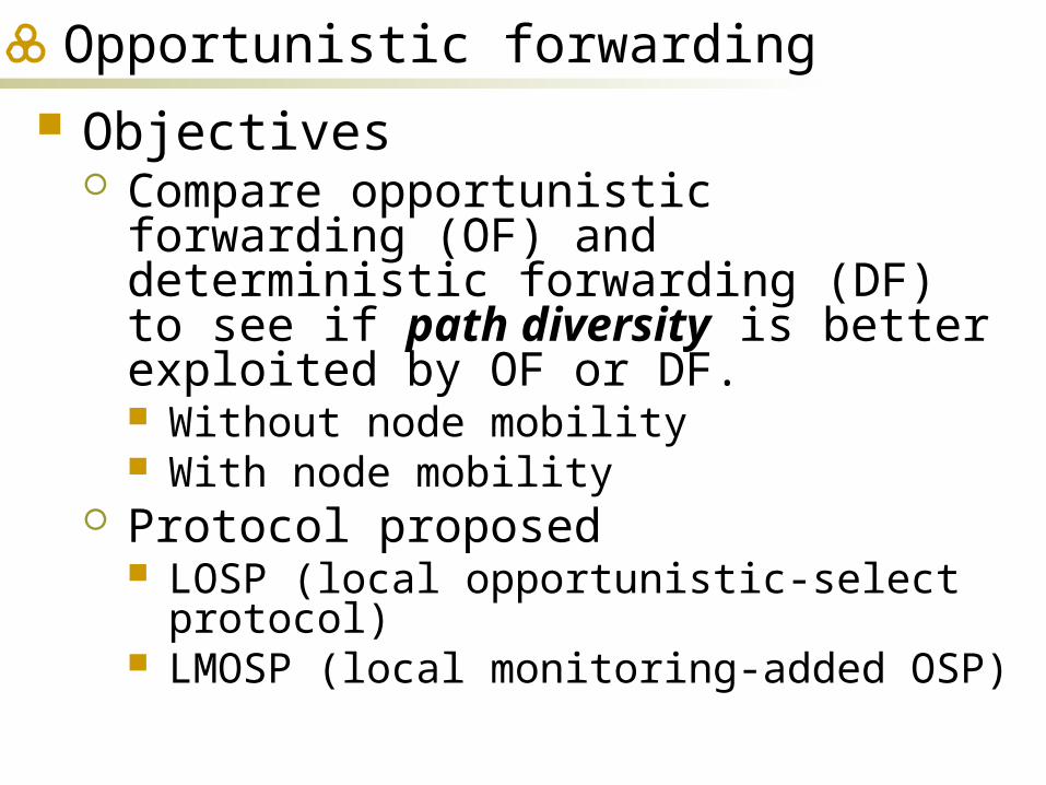
Opportunistic forwarding Objectives
Compare opportunistic forwarding (OF) and deterministic forwarding (DF) to see if path diversity is better exploited by OF or DF. Without node mobility With node mobility
Protocol proposed LOSP (local opportunistic-select protocol) LMOSP (local monitoring-added OSP)
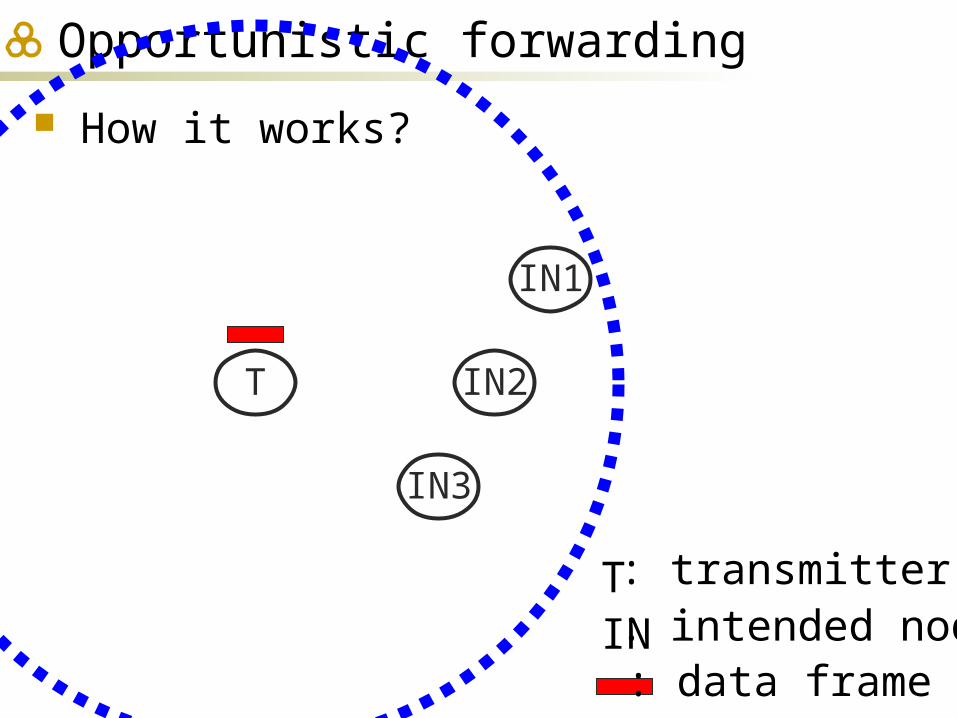
Opportunistic forwarding
How it works?
IN1
IN2T
IN3
: data frame
: transmitter: intended node
TIN
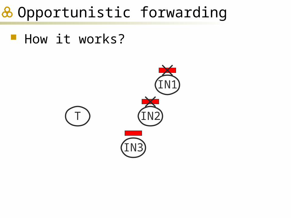
Opportunistic forwarding
How it works?
IN1
IN2T
IN3

Opportunistic forwarding
How it works?
IN1
IN2T
IN3
Priority : IN1 > IN2 > IN3

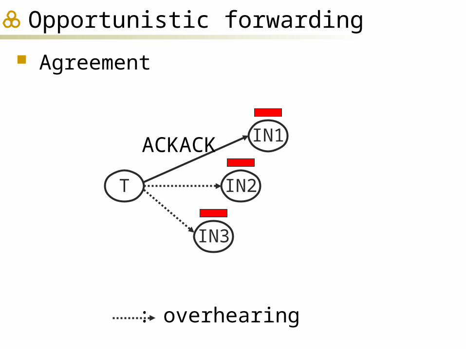
Opportunistic forwarding
Agreement
IN1
IN2T
IN3
ACK
: overhearing
Opportunistic forwarding
Agreement
IN1
IN2T
IN3
ACKACK
: overhearing

Opportunistic forwarding
Agreement
IN1
IN2T
IN3
ACK
: overhearing
obstacle
Opportunistic forwarding
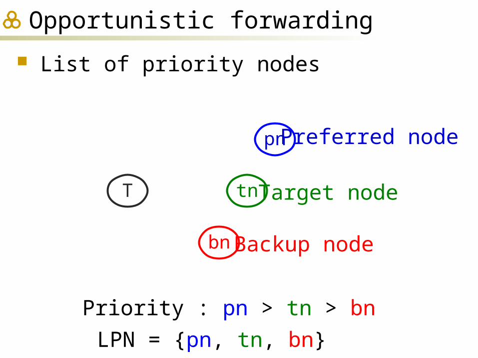
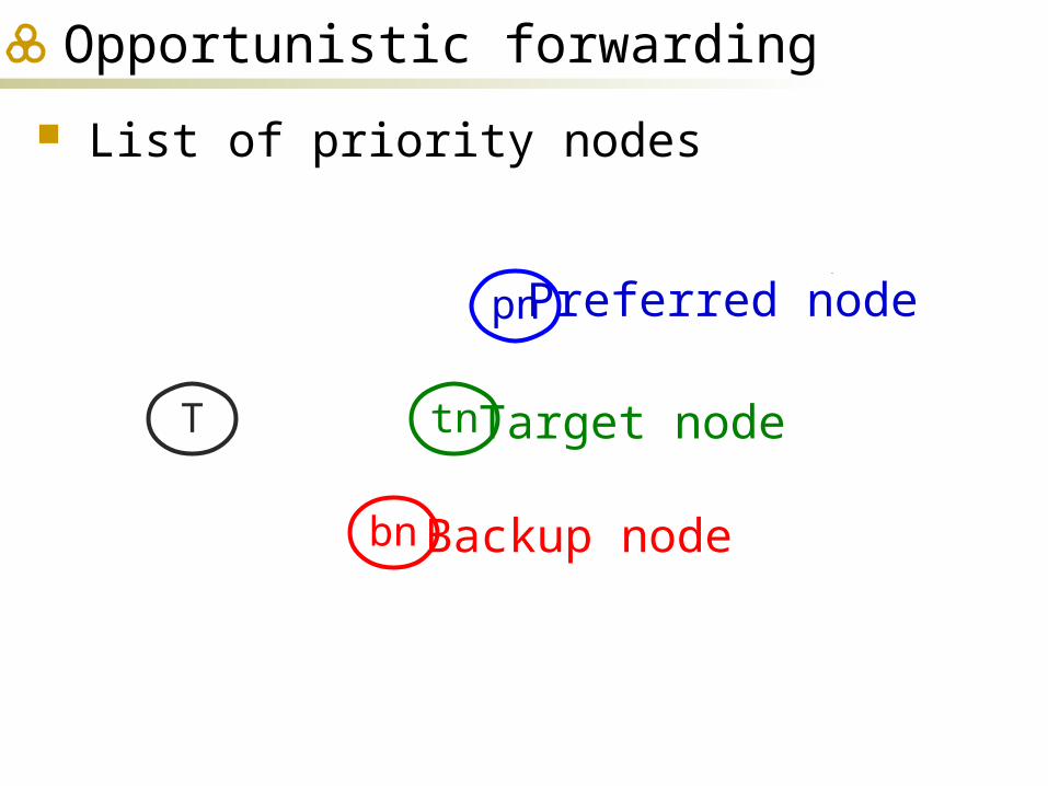
List of priority nodes
pn
tnT
bn
Preferred node
Target node
Backup node
Priority : pn > tn > bnLPN = {pn, tn, bn}
Opportunistic forwarding
List of priority nodes
T
Jdstpn Jdst
tn , SNRpnT SNRtn
T
Jdstbn Jdst
tn , SNRbnT SNRtn
T
pn
tn
bn
Preferred node
Backup node
Target node
Opportunistic forwarding
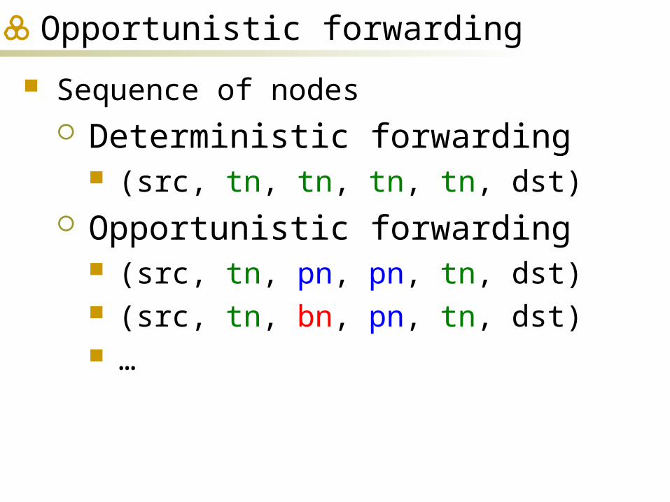
Sequence of nodes Deterministic forwarding
(src, tn, tn, tn, tn, dst) Opportunistic forwarding
(src, tn, pn, pn, tn, dst) (src, tn, bn, pn, tn, dst) …

Opportunistic forwarding
Bit-rate
bit-rateDF maxB
such that
fSNRTtn
, B THRESH
#
bit-rateOF maxB
such that
1 k pn or tn
1 fSNRTk , B THRESH
#
bit-rateDF bit-rateOF
Opportunistic forwarding
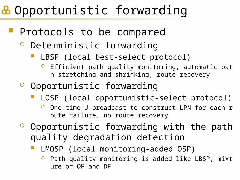
Protocols to be compared Deterministic forwarding
LBSP (local best-select protocol) Efficient path quality monitoring, automatic path stretching and sh
rinking, route recovery
Opportunistic forwarding LOSP (local opportunistic-select protocol)
One time J broadcast to construct LPN for each route failure, no route recovery
Opportunistic forwarding with the path quality degradation detection LMOSP (local monitoring-added OSP)
Path quality monitoring is added like LBSP, mixture of OF and DF

Opportunistic forwarding
Sequence of nodes Deterministic forwarding
(src, tn, tn, tn, tn, dst) Opportunistic forwarding
(src, tn, pn, pn, tn, dst) (src, tn, bn, pn, tn, dst) …
Opportunistic forwarding
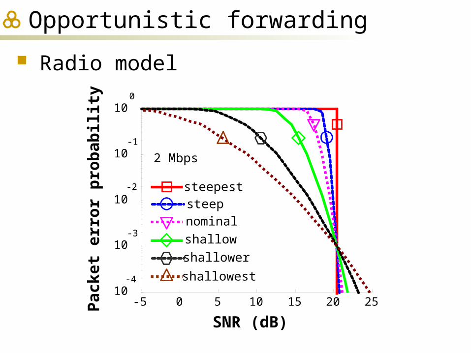
Radio modelP
acke
t er
ror
pro
bab
ilit
y
nominal
steepsteepest
shallowest
shallower
shallow
SNR (dB)-5 0 5 10 15 20 25
10-4
10-3
10-2
10-1
100
2 Mbps
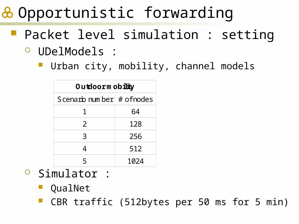
Opportunistic forwarding Packet level simulation : setting
UDelModels : Urban city, mobility, channel models
Simulator : QualNet CBR traffic (512bytes per 50 ms for 5 min)
Outdoor mobility
Scenario number # of nodes
1 64
2 128
3 256
4 512
5 1024
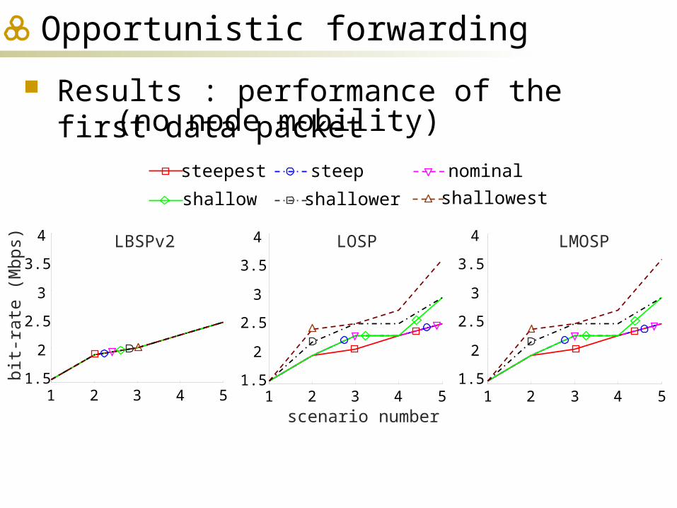
Opportunistic forwarding
Results : performance of the first data packet
1 2 3 4 51.5
2
2.5
3
3.5
4LBSPv2 LOSP LMOSP
nominalsteepsteepest
shallowershallow shallowest
1 2 3 4 51.5
2
2.5
3
3.5
4
1 2 3 4 51.5
2
2.5
3
3.5
4
scenario number
bit-
rate
(M
bps)
(no node mobility)

Opportunistic forwarding
Results : performance of the first data packet
nominalsteepsteepest
shallowershallow shallowest
1 2 3 4 522
23
24
25
26
27
scenario number1 2 3 4 5
22
23
24
25
26
27
1 2 3 4 522
23
24
25
26
27
SN
R (
dB)
LBSPv2 LOSP LMOSP
(no node mobility)

Opportunistic forwarding
Results : performance before the first route failure (node mobility involved)
nominalsteepsteepest
shallowershallow shallowest
scenario number
LBSPv2 LOSP LMOSP
1 2 3 4 51.5
2
2.5
3
3.5
1 2 3 4 51.5
2
2.5
3
3.5
bit-
rate
(M
bps)
1 2 3 4 51.5
2
2.5
3
3.5
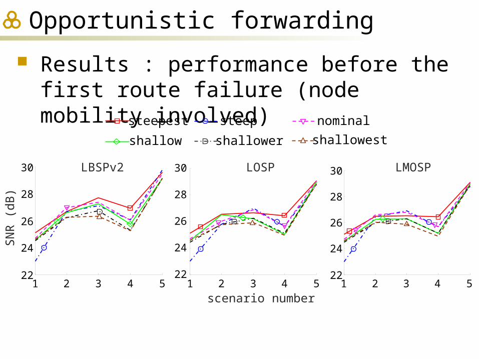
Opportunistic forwarding
Results : performance before the first route failure (node mobility involved)
nominalsteepsteepest
shallowershallow shallowest
scenario number
LBSPv2 LOSP LMOSP
SN
R (
dB)
1 2 3 4 522
24
26
28
30
1 2 3 4 522
24
26
28
30
1 2 3 4 522
24
26
28
30
Opportunistic forwarding
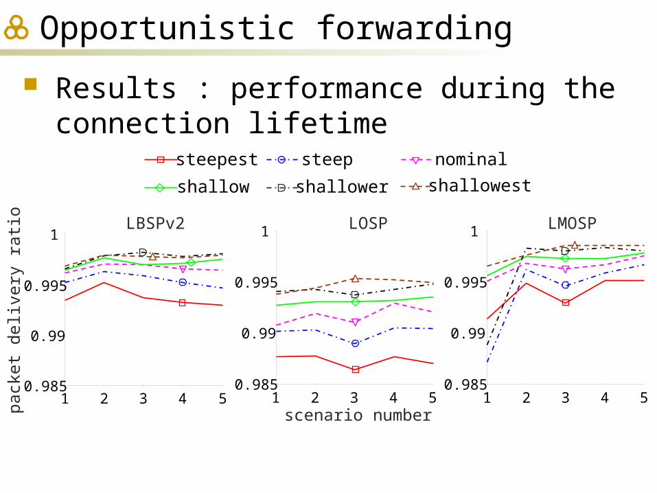
Results : performance during the connection lifetime
nominalsteepsteepest
shallowershallow shallowest
scenario number
LBSPv2 LOSP LMOSP
pack
et d
eliv
ery
ratio
1 2 3 4 50.985
0.99
0.995
1
1 2 3 4 50.985
0.99
0.995
1
1 2 3 4 50.985
0.99
0.995
1
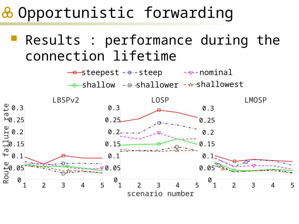
Opportunistic forwarding
Results : performance during the connection lifetime
nominalsteepsteepest
shallowershallow shallowest
LBSPv2 LOSP LMOSP
Rou
te f
ailu
re r
ate
scenario number1 2 3 4 5
0
0.05
0.1
0.15
0.2
0.25
0.3
1 2 3 4 50
0.05
0.1
0.15
0.2
0.25
0.3
1 2 3 4 50
0.05
0.1
0.15
0.2
0.25
0.3
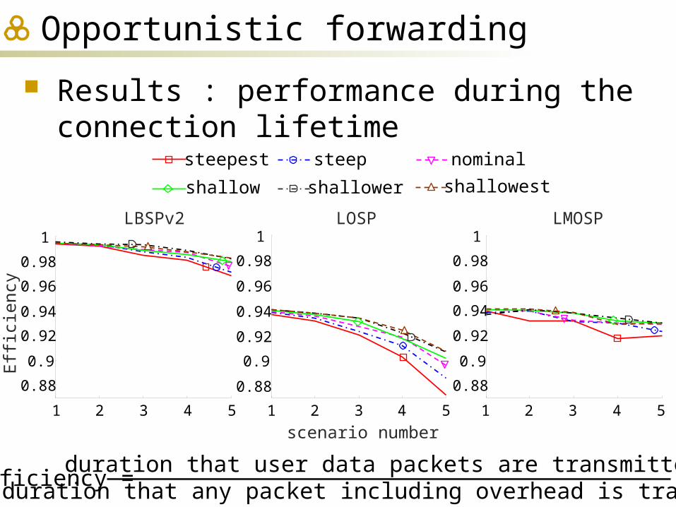
Opportunistic forwarding
Results : performance during the connection lifetime
nominalsteepsteepest
shallowershallow shallowest
LBSPv2 LOSP LMOSP
Eff
icie
ncy
scenario number1 2 3 4 5
0.88
0.9
0.92
0.94
0.96
0.98
1
1 2 3 4 5
0.88
0.9
0.92
0.94
0.96
0.98
1
1 2 3 4 5
0.88
0.9
0.92
0.94
0.96
0.98
1
duration that user data packets are transmittedduration that any packet including overhead is transmittedEfficiency =
Opportunistic forwarding
Conclusion Without mobility (e.g., stationary mesh network)
Opportunistic forwarding is preferred except for the overhead
With mobility Deterministic forwarding is preferred Path diversity is better exploited by deterministic
forwarding

Introduction and challenges Aggressive path quality monitoring
BSP Efficient path quality monitoring
LBSP Opportunistic forwarding
LBSP2, LOSP, LMOSP Conclusion and future work
Outline

Conclusions The significant benefits of path diversity are
possible using aggressive path quality monitoring.
Reducing overhead and advertising path quality efficiently are possible using the proposed novel techniques, still maintaining high benefits.
Path diversity is better exploited by deterministic forwarding with node mobility.
Conclusions and future work

Future work Estimate the dynamics of channel by observing
ongoing channel activity. Achieve fast estimation of link/path qualities
from the channel dynamic estimation. i.e., given the estimated current channel state,
estimate link/path qualities. Develop models of channel evolution.
Conclusions and future work

Schedule
Conclusions and future work
Date Task11/11/2011 11/20/2011∼ Packet level simulation11/21/2011 12/31/2011∼ Real channel measurement12/16/2011 12/31/2011∼ Develop models of channel
evolution01/01/2012 01/15/2012∼ Writing up all findings12/01/2011 01/31/2012∼ Proofreading the whole
thesis

Thanks