Explicit Newmark/Verlet algorithm forTime Integration of the

Rotational Dynamics of Rigid Bodies

P. Krysl∗, and L. Endres

April 20, 2004

Introduction

We consider the problem of integration of the initial value problem of the rotationalrigid body dynamics. We are motivated by a very practical problem: time integrationof the equations of motion of drill bits as they cut through rock. The drill bit geometryis fully three-dimensional, as is the surface of the rock to be cut, and the force laws ofcutting, scraping, impacts, and persistent contacts are heuristic, but computationallyintensive anyway. Consequently, evaluation of the forces acting at various points onthe bit is very expensive. (Similar observations may be made in many moleculardynamics simulations, where the evaluation of the forcing may take as much as 90%or more of the CPU time, or in finite element dynamics calculations.) Therefore itmakes eminent sense to try to limit the number of evaluations of the external torque,and we are thus led to consider methods that are explicit in the torque calculation,i.e. the torque is evaluated just once per time step, in preference to implicit methods(torque evaluated many times per time step).

We are generally looking for an integrator that is robust, accurate, and efficient.Conservation properties are often essential for the preservation of key qualitativefeatures of the motion. Equally important are often the dissipative and forcing char-acteristics [19]. In addition, three-dimensional rotations pose a special challenge inthat the configuration set is a curved manifold, not a vector space. The integratorshould maintain the configuration on the manifold. Methods for this type of problemhave been studied by many researchers, both in the computational mechanics com-munity, and in the applied mathematics community [5, 27, 1, 24, 20, 32, 21, 29, 25,42, 23, 8, 39, 2, 28, 10, 40, 22, 17, 33, 15, 41, 31, 26, 13, 6].

∗University of California, San Diego, 9500 Gilman Dr, La Jolla, CA 92093-0085,pkrysl@ucsd.edu

1

The issue of the integration of the equations of motion of a three-dimensionalrotating body may be approached from the general viewpoint of geometric integra-tion [4, 17]. A good example of a geometric integrator is the Verlet algorithm [38],whose generalization is the Newmark algorithm [30]. The Verlet/Newmark explicitintegrator has been recently shown to possess very attractive geometrical proper-ties [18, 19, 12]: Long-term energy and momentum near-conservation being perhapsthe most important for our applications. Simo and Wong [35] have studied the algo-rithms for rigid body rotation, and have proposed that the particular version of theiralgorithm which used β = 0 was the explicit Newmark. However, their algorithmdoes not display the same kind of behaviors that we see in the classical vector spaceversion of Newmark (crucially, it is not symplectic).

Our goal is to reformulate the traditional velocity based Newmark algorithm forvector spaces for the rotational dynamics of rigid bodies, that is for the setting of Liegroups. In fact, we show that the most naive re-write of the vector space algorithmdoes possess the desired properties, and is in fact one of the best-performing currentlyknown explicit algorithms for rigid body dynamics. Curiously, this algorithm doesnot seem to have been considered in the open literature at all. We claim that thisalgorithm is the true rotation-group counterpart of the vector space velocity-basedexplicit Newmark.

1 Formulation

In this section we very briefly present the formulation of the kinematics and dynamicsof the motion, chiefly to introduce the notation.

1.1 Kinematics

We shall consider rotations of a rigid body about a fixed point, located at the originof the global Cartesian system. An arbitrary particle in the reference configurationis addressed by the vector p0. The current position of the particle is expressed withthe current rotation (attitude) matrix R as

p = R · p0 (1)

where R is an orthogonal transformation, R−1 = RT .

1.1.1 Configuration

The orthogonal transformations R that represent rotations constitute points of aparticular manifold, the special orthogonal group SO(3). The motion of the rigidbody particles is therefore given as a mapping

t 7→ R ∈ SO(3) , (2)

2

where the presence of the special orthogonal group is what makes the problem ofdevising suitable integrators interesting.

The rotation matrix may be parameterized in many different ways [3]. In thiswork we use the rotation vector to express rotation matrices. Thus,

R(Ψ) =∞∑

k=0

Ψk

k!(3)

or, in the form of the Rodrigues formula

R(Ψ) = 1 +sin ||Ψ||||Ψ|| Ψ +

(1− cos ||Ψ||)||Ψ||2 Ψ

2. (4)

When needed, the rotation vector may be extracted from the rotation matrix withthe Spurrier’s algorithm (see for instance reference [34]).

1.1.2 Velocity

The velocity vector of a given particle is obtained from (1) as

˙p = Rp0 . (5)

We may defineR = RΩ (6)

where Ω is the body-attached (convected) angular velocity. The wave symbol is usedto indicate a skew-symmetric matrix, which is related to the angular velocity Ω as avector through Ω ·Ω = 0.

Alternatively, the time derivative (6) may be expressed as

R = ωR (7)

where ω is the spatial angular velocity as a skew-symmetric matrix; the spatial vectorof angular velocity ω is defined as ω · ω = 0.

Skew-symmetric matrices are elements of the vector space

so(3) =

h : R3 7→ R3|h + hT

= 0

(8)

with a map into R3 defined ashv = h× v (9)

The spatial and the convected angular velocity are related through the two equiv-alent relations

ω = RΩRT and ω = RΩ . (10)

The velocity of a given particle in the body may thus be written as

˙p = RΩp0 = ωRp0 (11)

3

1.1.3 Angular acceleration

Proceeding with time differentiation, we obtain for the acceleration

¨p = R(Ω2+ A)p0 = (ω2 + α)Rp0 (12)

where A is the body frame (convected) angular acceleration as a skew-symmetric

tensor, A =˙Ω; α is the spatial angular acceleration as a skew-symmetric tensor,

α = ˙ω.

1.2 Dynamics

1.2.1 Principle of Virtual Power

The virtual velocity may be written as

η = RHΩp0 = −R ˜p0HΩ (13)

where HΩ is the virtual angular velocity in the body frame.

1.2.2 Virtual power of the inertial forces

The virtual power of the inertial forces may be written as

Pi =

∫

V

η · ρ¨p dV (14)

where η is the virtual velocity; ρ is the mass density; and V is the volume of thebody.

Pi =∫

V(R ˜p0HΩ) · ρ(R(Ω

2+ A)p0) dV

=∫

V(R ˜p0HΩ) · ρ(R(−Ω ˜p0Ω− ˜p0A)) dV

(15)

which may be put into a familiar form using the tensor of inertia

Pi = HΩ · Ω∫

Vρ ˜p0

T ˜p0 dV Ω + HΩ ·∫

Vρ ˜p0

T ˜p0 dV A

= HΩ · ΩIΩ + HΩ · IA(16)

where I =∫

Vρ ˜p0

T ˜p0 dV is the tensor of inertia in the body frame.

1.3 Virtual power of the applied forces

For a given force f applied at the point q, the virtual power may be written as

Pe = η · f = (R ˜q0HΩ) · f = HΩ ˜q0 ·RT f = HΩ · T (17)

where T = ˜q0 ·RT f is the torque in the body frame.

4

1.4 Equation of motion

The equation of motion follows from the principle of virtual power as

Pi = Pe (18)

or explicitly

ΩIΩ + IA = T (19)

The above equation of motion in the body frame may be also cast in the spatialframe

ωiω + ia = t (20)

where i = RIRT is the tensor of inertia in the spatial frame; and t = RT is thetorque in the spatial frame.

2 Time Discretization

The classical Newmark integration algorithm is formulated as follows, using two pa-rameters, γ and β [30]

∆qn = ∆tvn−1 +∆t2

2[(1− 2β)an−1 + 2βan] (21)

vn = vn−1 + ∆t [(1− γ)an−1 + γan] (22)

where ∆qj = qj − qj−1 is the increment of the algorithmic position vector at timetj; vj is the algorithmic velocity of the vector qj at time tj; aj is the algorithmicacceleration of the vector qj at time tj. Note that all the vectors qj, vj, and aj mustbelong to a vector space S,

qj ∈ S, vj ∈ S, aj ∈ S

in order for the linear combination in equations (21,22) to make sense.For the particular choice β = 0 the Newmark algorithm becomes explicit:

∆qn = ∆tvn−1 +∆t2

2an−1 (23)

vn = vn−1 + ∆t [(1− γ)an−1 + γan] (24)

2.1 Compound rotations and tangents

While the increment ∆qn = qn − qn−1 may be expressed as a difference of twoconfigurations (locations) in (23), the transition in SO(3) from the rotation Rn−1 tothe rotation Rn needs to be computed in terms of compound rotations.

A compound rotation curve may be constructed from a given rotation R eitherby left or right multiplication with another finite rotation matrix, parameterized with

5

the scalar ε. Left multiplication by the matrix δR corresponds to an incrementalrotation applied in the spatial setting

R′ = δR ·R , (25)

right multiplication by the matrix ∆R corresponds to an incremental rotation appliedin the body-frame setting

R′ = R ·∆R (26)

The incremental matrices are expressible as rotations about a given, fixed (rotation)vector. Thus, the left incremental rotation δR may be written as

δR = exp[εδψ] , (27)

and the right incremental rotation ∆R may be written as

∆R = exp[ε∆Ψ] . (28)

Tangent vectors to the compound curves may be evaluated as

dR′

dε|ε=0 = δψR = R∆Ψ (29)

2.2 Rotation update

For now we shall proceed with formulation in the body frame. The incremental vector∆Ψ belongs to a vector space, the tangent space TRSO(3) to the manifold SO(3) atthe rotation R

∆Ψ ∈ TRSO(3) .

Both the body-frame angular velocity Ω, and angular acceleration A belong also tothe same vector space

Ω ∈ TRSO(3), A ∈ TRSO(3) .

Notice that all quantities in equation (23) are expressed in the same configuration attime tn−1. Therefore, it makes sense to construct the incremental rotation vector ∆Ψn

that will take us from the rotation Rn−1 to the rotation Rn by combining the angularvelocity and the angular acceleration. In other words, the Newmark algorithm maybe applied in the vector space TRn−1SO(3), so that equation (23) may be specializedas

∆Ψn = ∆tΩn−1 + ∆t2

2An−1, (30)

and the configuration will be therefore updated as

Rn = Rn−1 exp[∆Ψn] .

6

2.3 Angular velocity update

Now we proceed to the second Newmark equation, the update of the angular ve-locity (24). At variance with (23), this equation mixes together accelerations andvelocities from two different time steps, and hence belonging to two different tangentspaces. Therefore, we need to introduce the concept of the dexp operator (differ-ential of the exponential map) [17]. For the case of rotations in 3-D, we may referfor instance to [5], and relate increments to rotation vectors in two different tangentspaces, at RA and RB = RA exp(Ψ). We express a curve RB,ε using increments inthe two tangent spaces, ΘA ∈ TRA

SO(3) and ΘB ∈ TRBSO(3)

RB,ε = RA exp(Ψ + εΘA) = RB exp(εΘB) (31)

As shown in Reference [5], the two rotation vectors may be then related as

ΘB = S(Ψ)ΘA, (32)

where the operator that relates the two tangent spaces is

dexpΨ = S(Ψ) = 1 +1− cos ||Ψ||||Ψ||2 Ψ +

(1− sin ||Ψ||

||Ψ||)

Ψ2

||Ψ||2 . (33)

Relation (32) may be applied to the construction of the update of angular veloci-ties. For instance, we could push forward quantities from configuration at time tn−1

to configuration at tn by the rotation increment ∆Ψn, which yields

Ωn = S(∆Ψn)Ωn−1 + ∆t [(1− γ)S(∆Ψn)An−1 + γAn] (34)

We could stop here, but there’s more that can be done. If we rewrite equation (34)as

Ωn = S(∆Ψn) [Ωn−1 + ∆t(1− γ)An−1] + ∆tγAn , (35)

we may realize that the contents of the bracket are co-axial with the incrementalrotation vector ∆Ψn from equation (30), provided γ = 1/2. Thus, for this choice ofthe coefficient γ, the shift with S(∆Ψn) has no effect [hint: use equation (9)], andmay be omitted. Since the choice of γ = 1/2 is known to be optimal from the pointof view of accuracy, it also appears in the Verlet algorithm, and we are going to usethis numerical value too. Therefore, we shall be using

Ωn = Ωn−1 +∆t

2(An−1 + An) , (36)

as the angular velocity update equation.

7

2.3.1 Evaluated acceleration

The last essential component of the algorithm (21) is the algorithmic (evaluated)acceleration, which is readily obtained from the equation of motion (19). As willbecome clear in a moment, we need to solve a system of nonlinear equations to obtainthe acceleration, since it is coupled with the angular velocity due to the velocityupdate.

The three ingredients, the configuration update, the velocity update, and the useof the evaluated acceleration combine, in some way that might not be at this pointcompletely understood, to balance good behaviors (energy and momentum represen-tation) in a nearly optimal way.

2.4 Explicit Newmark algorithm in the body frame

To summarize equations (30) and (36), the explicit Newmark algorithm (β = 0, andγ = 1/2) in the body frame (NMB) may be written as

Algorithm NMB:Given Ω0, R0,A0 = I−1(RT

0 T 0 −Ω0 × I ·Ω0)for n = 1, 2, ...

Rn = Rn−1 exp[∆tΩn−1 + ∆t2

2An−1]

IAn −RTnT n + Ωn × I ·Ωn = 0

Ωn = Ωn−1 + ∆t2

(An−1 + An)end

Note that the algorithm is self-starting, which is particularly nice from the pointof view of implementation. The integrator algorithm may be called repeatedly withthe output of the previous invocation as the initial conditions, and there will be noloss of accuracy involved in doing so.

Also of note is the fact that we never actually need the components of the rotationvector (or those of the associated quaternion): the update is performed on the ro-tation matrix, and in our numerical experiments we have not come across numericaldifficulties. However, should such a need arise it is always possible to re-orthogonalizeR, or extract the rotation vector components. Of course, that is what we have to dowhen the rotation vector components, or the components of the incremental rotationvector are needed for output.

2.5 Explicit Newmark algorithm in the spatial frame

Contrary to popular belief, the spatial form of the above body-frame Newmark al-gorithm as given below makes geometric sense and is completely equivalent to thebody-frame version.

8

Algorithm NMS:Given ω0,R0,α0 = i−1

0 (t0 − ω0 × i0 · ω0)for n = 1, 2, ...

Rn = exp[∆tωn−1 + ∆t2

2αn−1]Rn−1

inαn − tn + ωn × in · ωn = 0ωn = ωn−1 + ∆t

2(αn−1 + αn)

end

To show the equivalence, we may start with the rotation update equation and tosubstitute the convected angular velocity and convected angular acceleration

Rn = Rn−1 exp[∆tΩn−1 + ∆t2

2An−1]

= Rn−1

∞∑

k=0

(∆tΩn−1 + ∆t2

2An−1)

k

k!

= Rn−1

∞∑

k=0

(∆tRTn−1ωn−1Rn−1 + ∆t2

2RT

n−1αn−1Rn−1)k

k!

=∞∑

k=0

(∆tωn−1 + ∆t2

2αn−1)

k

k!Rn−1

= exp[∆tωn−1 + ∆t2

2αn−1]Rn−1

(37)

Analogously, we obtain the spatial version of the equation of motion

IAn −RTnT n + Ωn × I ·Ωn =

RTn inαn −RT

nT n + RTnωn × in · ωn = 0

(38)

where we have to substitute for the angular velocity at time tn from

Ωn = Ωn−1 + ∆t2

(An−1 + An)= RT

nωn = RTn−1ωn−1 + ∆t

2(RT

n−1αn−1 + RTnαn)

(39)

Thus, we obtain

ωn = RnRTn−1ωn−1 +

∆t

2(RnR

Tn−1αn−1 + αn) (40)

However, from equation (37) we have RnRTn−1 = exp[∆tωn−1+

∆t2

2αn−1]. To complete

the proof, we need to realize that the vector ωn−1 + ∆t2

αn−1 is a scalar multiple of

the axial vector of the rotation matrix exp[∆tωn−1 + ∆t2

2αn−1], and is not affected by

the rotation, and therefore

ωn = exp[∆tωn−1 +∆t2

2αn−1](ωn−1 +

∆t

2αn−1) +

∆t

2αn

= ωn−1 +∆t

2(αn−1 + αn)

(41)

9

2.6 Solving the equation of motion

Note that both algorithms NMB and NMS need to obtain the angular accelerationsby solving a nonlinear algebraic equation. For instance, for the algorithm NMS thefollowing equation in residual form needs to be solved

R(αn) = Inαn − T n + ωn × In · ωn = 0 (42)

where ωn = ωn−1 + ∆t2

(αn−1 + αn), or; ωn = ωn,p + ∆t2

αn, with the definitionωn,p = ωn−1 + ∆t

2αn−1. We may write a straightforward Newton’s solver as

α(0)n = 0, i = 1

while ‖R(α(i−1)n )‖ > TOL

α(i)n = α

(i−1)n −

[∂R(α

(i−1)n )

∂αn

]−1

R(α(i−1)n )

end

with the tangent ∂R/∂αn

∂R(α(i−1)n )

∂αn

= In +∆t

2

(ωn,pIn − Inωn,p

)+

∆t2

2

(αnIn − Inαn

)(43)

3 Numerical Experiments

We are going to compare the performance of the Newmark algorithm (NMB, NMS)with the performance of the two top-performing explicit algorithms, the staggeredmomentum-conserving explicit algorithm [16] (HSTAGM) (see also discussion inSvanberg [36]), and the explicit time integration algorithm of Simo and Wong [35](SW). For reader’s convenience, both algorithms are summarized in the Appendix A.For comparison we also include references to the canonical implicit midpoint almost-Lie-Poisson algorithm of Austin, Krishnaprasad, Wang [1] (AKW).

3.1 Freely spinning body (McLachlan, Zanna 2003)

This example is discussed in the report [26] in the context of discrete Moser-Veselovintegrators for the rigid body. The initial condition is Ω = (0.45549, 0.82623, 0.03476),and the diagonal entries of the inertia tensor are diagI = (0.9144, 1.098, 1.66).

Figure 1 demonstrates how well-behaved the Newmark algorithm is in terms ofkinetic energy. Even though the kinetic energy is not conserved, it oscillates withunchanging amplitude and without drift. Note that the time steps are quite large,which can be clearly seen in Figure 2 showing the magnitude of the incrementalrotation vector in degrees.

Figure 3 shows the components of the body-frame angular velocity. One can seethat the qualitative character is very well preserved even for large time steps. This

10

0 20 40 60 80 1000.4

0.41

0.42

0.43

0.44

0.45

0.46

0.47

0.48

0.49

Time

Kin

etic

ene

rgy

Figure 1: Freely spinning rigid body; kinetic energy for a step sizes 4 (), 2 (×), 1(?), 1/2 (¤).

0 20 40 60 80 1000

50

100

150

Time

Mag

nitu

de o

f inc

rem

enta

l rot

atio

n ve

ctor

Figure 2: Freely spinning rigid body; magnitude of the incremental rotation vectorin degrees for step sizes 4 (), 2 (×), 1 (?), 1/2 (¤).

11

0 20 40 60 80 100−1

−0.8

−0.6

−0.4

−0.2

0

0.2

0.4

0.6

0.8

1

Time

Ang

ular

vel

ocity

/bod

y fr

ame

Ω1

Ω2

Ω3

Figure 3: Freely spinning rigid body; components of the body-frame angular velocityfor a step sizes 5 (), 4 (×), 2 (?), 1/8 (¤).

is a very attractive feature of the present Newmark algorithm. When compared withother algorithms discussed in reference [26] in figure 7.7, for the largest timestep,∆t = 5, our algorithm performs on par with the implicit midpoint rule (IMR, ourAKW) which is the only one that is able to capture the character of the solution,while all the discrete Moser-Veselov integrators fail.

Figure 4 shows the convergence of the Newmark algorithm in the norm ||R −Rconverged||2, where the orientation matrix Rconverged = R(t = 100) has been obtainedwith an extremely small step size of 0.001. Note that our algorithm outperforms theAKW by two orders of magnitude.

3.2 Unstable rotation: book toss

Consider a body described in the body frame whose directions coincide with theprincipal directions of the tensor of inertia. It is well known that if the three principalvalues of the tensor of inertia are different, rotation about the axis corresponding tothe intermediate principal value is unstable [37]. Real world examples include thetoss of a book. When the book is tossed with a spin imparted about the intermediateaxis, the book will as likely as not flip in mid-flight due to the slightest disturbance.

The data for this example appear to be due to Simo and Wong [35]. It hadalso been studied by Hulbert [16]. A constant torque is applied about the axis ofintermediate moment of inertia to a body that is initially at rest. Then, at timet = td, the constant torque is removed and a constant disturbance torque is appliedabout an axis perpendicular to that of the intermediate moment of inertia for theduration of a single timestep ∆t. The body frame tensor of inertia is diagonal,diagI = (5, 10, 1). The spatial components of the torque are

(20, 0, 0), for 0 ≤ t ≤ td;(0, 1/(5∆t), 0), for td ≤ t ≤ td + ∆t;(0, 0, 0), for t >= td + ∆t.

12

10−3

10−2

10−1

100

101

10−6

10−5

10−4

10−3

10−2

10−1

100

101

log(step size)

log(

||R−

Rco

nver

ged||)

HSTAGM

SW

NMB

AKW

Figure 4: Freely spinning rigid body; convergence in the norm ||R − Rconverged||.Thick solid line () present Newmark (NMB); thick dotted line Simo-Wong explicitalgorithm (SW); thick dash-dot line Lewis-Simo implicit algorithm (LS): for stepsizes 8, 4, 2, 1, 1/2, 1/4, 1/8, 1/16, 1/32, 1/64, 1/128, and 1/256;.

10−3

10−2

10−1

100

101

10−6

10−5

10−4

10−3

10−2

10−1

100

101

log(step size)

log(

||Π−

Πco

nver

ged||)

HSTAGM

SW NMB

AKW

DMV

LP2

Figure 5: Freely spinning rigid body; convergence in the body-frame momenta, norm||M −M converged||. Thick line (, (NMB)): Newmark for step sizes 8, 4, 2, 1, 1/2,1/4, 1/8 and 1/16 (1/32, 1/64, 1/128, 1/256); thick dotted line Simo-Wong explicitalgorithm (SW); thick dash-dot line Lewis-Simo implicit algorithm (LS); (∗): LP2(explicit Lie-Poisson integrator of the second order); (/): IMR (implicit midpointrule); (?): DMV (discrete Moser-Veselov); (♦): DMV4 (fourth order discrete Moser-Veselov); (×): DMV6 (sixth order discrete Moser-Veselov).

13

0 2 4 6 8 10−15

−10

−5

0

5

10

Time

Ang

ular

vel

ocity

/bod

y fr

ame

Ω1

Ω2

Ω3

0 2 4 6 8 10−15

−10

−5

0

5

10

Time

Ang

ular

vel

ocity

/bod

y fr

ame

Ω1

Ω2

Ω3

Figure 6: Book toss; convected angular velocities; left: NMB time step 0.05 (), and0.001 (×), right: SW time step 0.05 (), and 0.001 (×).

0 2 4 6 8 10−10

−5

0

5

10

15

20

25

30

35

40

Time

Spa

tial A

ngul

ar m

omen

ta

π1

π2

π3

0 2 4 6 8 10−10

−5

0

5

10

15

20

25

30

35

40

Time

Spa

tial A

ngul

ar m

omen

taπ

1π

2π

3

Figure 7: Book toss; spatial angular momenta; left: NMB time step 0.05 (), and0.001 (×), right: SW time step 0.05 (), and 0.001 (×).

In Figure 6 the characteristic pattern of the body-frame angular velocities is dis-played for two different time steps. The tendency of the SW algorithm to becomeunstable for larger time steps is quite clearly visible. On the other hand, the New-mark algorithm does not seem to have any trouble maintaining stability, and eventhe accuracy of the angular velocities seems quite acceptable.

Conservation of the angular momentum is illustrated in Figure 7: the Newmarkalgorithm clearly does not conserve momenta exactly, however, the conservation isachieved in a different sense. The oscillations of the momenta are limited, and seemto be more or less periodic in time. On the other hand, the SW algorithm conservesmomenta exactly, even in those cases where it is actually unstable. This only illus-trates that the conservation of momenta on its own does not necessarily mean thatgood results follow.

14

0 20 40 60 80 100−0.05

−0.04

−0.03

−0.02

−0.01

0

0.01

Time

Err

or in

Ham

ilton

ian

Error in Hamiltonian

Figure 8: Lagrangian top; error in the Hamiltonian.

3.3 Lagrangian top

This particular problem had been studied with the number of methods [11, 9]. It iswell known that the symmetric Lagrangian heavy top model possesses four conservedquantities:

1. the Hamiltonian,

H(π, γ) =1

2π · i−1π + Mlgγ · χ

where π is the spatial angular momentum, π = π ·ω; χ is the unit vector alongthe axis of the top pointing from the fixed point; γ is the unit vector in thedirection of gravity; Mlg is the product of the mass, distance of the center ofmass and the fixed point, and gravitational acceleration, Mlg =

√3

29.81.

2. the projection of the spatial angular momentum on the axis of the top, π · χ,

3. the projection of the spatial angular momentum on the gravity vector, π · γ,

4. the norm of the gravity vector in the body frame, ||Rγ||.The last two are the Casimirs of the Poisson bracket that defines the Hamiltonianstructure.

The step size of the integration was ∆ = 0.05, and the dynamics was integratedon the interval 0 ≤ t < 100. The error in Hamiltonian is shown in Figure 8. Noticethat the error in the Hamiltonian does not drift and stays fairly small (less than halfa percent of the exact Hamiltonian).

The algorithm NMB (NMS) is about as accurate both in the preservation of theinvariants and in the global error (convergence curve constant as well as slope) as theCrouch-Grossman method [7] with the Runge-Kutta RK4 tableau [11].

The projection of the spatial angular momentum onto the axis of the top is shownin Figure 9. The two curves correspond to a simulation which performs the rotation

15

0 20 40 60 80 100−8

−6

−4

−2

0

2

4

6

8x 10

−14

Time

<π,

χ>

<π,χ>

Figure 9: Lagrangian top; error in the projection of the spatial angular momentumonto the axis of the top.

update directly on the attitude matrix by matrix-matrix multiplication (larger error),and to a simulation in which the attitude matrix is re-orthogonalized in each timestep.Clearly, the error is then down to machine precision. Hardly any effect may be seenfor either simulation in the physical characteristics of the motion, however.

3.4 Fast Lagrangian top

The data for this example appear to be due to Simo and Wong [35]. It had also beenstudied by Hulbert [16]. In this example we consider the motion of a symmetrical topwith total mass M and axis of symmetry that coincides with the direction of uniformgravitational field. The body frame tensor of inertia is diagonal, diagI = [5, 5, 1].The spatial torque is

t = −20R(:, 3)× [0; 0; 1]

where R(:, 3) is the third column of the attitude matrix, and [0; 0; 1] is the “up” vector.

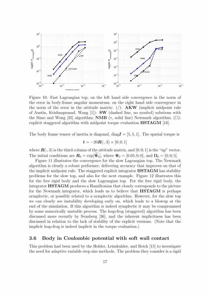
The initial conditions are R0 = exp[Ψ0] where Ψ0 = [0.3; 0; 0], and Ω0 = [0; 0; 50].We investigate the global convergence by using a numerical solution (obtained withan extremely small timestep ∆t = 0.000005) for the attitude matrix and the bodyframe angular momenta at time t = 10. We measure the norm ||R−Rconverged||2, andthe norm ||Π − Πconverged||2, where the reference values are the orientation matrixRconverged = R(t = 10) and the body frame angular momentum Πconverged = Π(t =10). The convergence curves are shown in Figure 10. The SW and HSTAGMalgorithms yield essentially identical answers except for the largest time steps.

3.5 Slow Lagrangian top

In this example we consider the motion of a slow symmetrical top with total mass Mand axis of symmetry that coincides with the direction of uniform gravitational field.

16

10−4

10−3

10−2

10−1

10−3

10−2

10−1

100

101

log(time step)

log(

||Π−

Πco

nver

ged||)

SW

HSTAGM

AKW

NMB

10−4

10−3

10−2

10−1

10−5

10−4

10−3

10−2

10−1

100

101

log(

||R−

Rco

nver

ged||)

SW

HSTAGM

NMB

AKW

Figure 10: Fast Lagrangian top; on the left hand side convergence in the norm ofthe error in body-frame angular momentum; on the right hand side convergence inthe norm of the error in the attitude matrix: (/): AKW (implicit midpoint ruleof Austin, Krishnaprasad, Wang [1]): SW (dashed line, no symbol) solutions withthe Simo and Wong [35] algorithm; NMB (, solid line) Newmark algorithm; (¤):explicit staggered algorithm with midpoint torque evaluation HSTAGM [16].

The body frame tensor of inertia is diagonal, diagI = [5, 5, 1]. The spatial torque is

t = −20R(:, 3)× [0; 0; 1]

where R(:, 3) is the third column of the attitude matrix, and [0; 0; 1] is the “up” vector.

The initial conditions are R0 = exp[Ψ0], where Ψ0 = [0.05; 0; 0], and Ω0 = [0; 0; 5].Figure 11 illustrates the convergence for the slow Lagrangian top. The Newmark

algorithm is clearly a robust performer, delivering accuracy that improves on that ofthe implicit midpoint rule. The staggered explicit integrator HSTAGM has stabilityproblems for the slow top, and also for the next example. Figure 12 illustrates thisfor the free rigid body and the slow Lagrangian top. For the free rigid body, theintegrator HSTAGM produces a Hamiltonian that closely corresponds to the picturefor the Newmark integrator, which leads us to believe that HSTAGM is perhapssymplectic, or possibly related to a symplectic algorithm. However, for the slow topwe can clearly see instability developing early on, which leads to a blowup at theend of the simulation. If this algorithm is indeed symplectic it may be compromisedby some numerically unstable process. The leap-frog (staggered) algorithm has beendiscussed more recently by Svanberg [36], and the inherent implicitness has beendiscussed in relation to the lack of stability of the explicit versions. (Note that theimplicit leap-frog is indeed implicit in the torque evaluation.)

3.6 Body in Coulombic potential with soft wall contact

This problem had been used by the Holder, Leimkuhler, and Reich [15] to investigatethe need for adaptive variable step size methods. The problem they consider is a rigid

17

10−3

10−2

10−1

10−5

10−4

10−3

10−2

10−1

100

101

102

log(

||Π−

Πco

nver

ged||)

HSTAGM

SWAKW

NMB

10−3

10−2

10−1

10−4

10−3

10−2

10−1

100

101

log(time step)

log(

||R−

Rco

nver

ged||)

HSTAGM

SW AKW

NMB

Figure 11: Slow Lagrangian top; on the left hand side convergence in the norm ofthe error in body-frame angular momentum; on the right hand side convergence inthe norm of the error in the attitude matrix: (/): AKW (implicit midpoint ruleof Austin, Krishnaprasad, Wang [1]): SW (dashed line, no symbol) solutions withthe Simo and Wong [35] algorithm; NMB (, solid line) Newmark algorithm; (¤):explicit staggered algorithm with midpoint torque evaluation HSTAGM [16].

0 100 200 300 400 500

0.47

0.472

0.474

0.476

0.478

0.48

Time

Kin

etic

ene

rgy

HSTAGM

NMB

SW

0 5 10 15

32.41

32.42

32.43

32.44

32.45

32.46

32.47

32.48

32.49

32.5

32.51

Time

Ham

ilton

ian

SW

HSTAGM

NMB

Figure 12: Free rigid body and Slow Lagrangian top Hamiltonians: SW (dashedline, no symbol) solutions with the Simo and Wong [35] algorithm; NMB (, solidline) Newmark algorithm; (¤): explicit staggered algorithm with midpoint torqueevaluation HSTAGM [16].

body that rotates under an external torque coming from an attractive Coulombicpotential coupled with a repulsive potential with steep gradient that represents a softwall from which the rotating body is repeatedly repelled. As the authors point out,the repelling torque is troublesome from the point of view of resolution.

The body frame tensor of inertia is diagonal, diagI = [2, 3, 4.5]. The components

18

of the spatial torque are

[t] =(−(1.1 + R3,3)

−2 + 0.01(1.1 + R3,3)−11

)[−R2,3; R1,3; 0]

where Rij are the components of the attitude matrix. The initial conditions areR0 = 1, and π0 = [2; 2; 2].

Figure 13 compares the convergence of the various algorithms discussed here.The Newmark algorithm clearly outperforms all the others, including the canonicalimplicit midpoint method.

10−2

10−1

100

10−3

10−2

10−1

100

101

log(time step)

log(

||Π−

Πco

nver

ged||)

SW

AKW

NMBHSTAGM

10−2

10−1

100

10−2

10−1

100

101

log(time step)

log(

||R−

Rco

nver

ged||)

SW NMB

AKWHSTAGM

Figure 13: Body in Coulombic potential with soft wall contact; on the left handside convergence in the norm of the error in body-frame angular momentum; on theright hand side convergence in the norm of the error in the attitude matrix: (/):AKW (implicit midpoint rule of Austin, Krishnaprasad, Wang [1]): SW (dashedline, no symbol) solutions with the Simo and Wong [35] algorithm; NMB (, solidline) Newmark algorithm; (¤): explicit staggered algorithm with midpoint torqueevaluation HSTAGM [16].

Discussion

The explicit Newmark algorithms discussed here, namely NMB, and NMS, andalso the SW algorithm, are time symmetric (for background see for example [14]).To show that for instance for the proposed Newmark algorithm, we need to swapsubscripts n and n − 1 and change the sign of the time step. Thus, the rotationupdate

Rn = Rn−1 exp[∆tΩn−1 +∆t2

2An−1] (44)

will become after the swap

Rn−1 = Rn exp[−∆tΩn +∆t2

2An] (45)

19

while the angular velocity update

Ωn = Ωn−1 +∆t

2(An−1 + An) (46)

will read

Ωn−1 = Ωn − ∆t

2(An + An−1) (47)

However, we may express

Ωn−1 +∆t

2An−1 = Ωn − ∆t

2An

which upon substitution into (45) yields algorithm identical to equations (44), (46).As pointed out for some integrators [41], time symmetry often leads to good energybehavior. However, clearly that is not a sufficient condition since the Simo and Wongintegrator displays a drift in energy for all time steps.

It would appear that the present Newmark is a symplectic integrator. A proofhas not been completed yet, but the numerical evidence is very strong.

Conclusions

We have explored the issue of time stepping for the dynamics of rigid bodies inthree-dimensional space with explicit time integrators. In particular, we show thatthe most naive and straightforward rewrite of the Verlet/Newmark algorithm for therotation group inherits a collection of good behaviors essentially analogous to thoseof the vector-space version. On the other hand, the explicit momentum-conservationalgorithm as proposed by Simo and Wong [35] that is sometimes referred to as animplementation of the explicit Newmark does not display the characteristics we wouldexpect.

We propose that our algorithm is the explicit velocity-based Newmark for therotation dynamics setting. It is a very good performer, robust and accurate. Inways that are likely not fully understood at this moment it manages to balance goodbehaviors in momentum and energy representation.

ACKNOWLEDGMENTS

This research was partially supported by a Hughes-Christensen research award. Thissupport is gratefully acknowledged. The author wishes to thank Jerry Marsden forinsightful comments and suggestions.

References

[1] M. Austin, P. S. Krishnaprasad, and L. S. Wang. Almost Lie-Poisson integratorsfor the rigid body. Journal of Computational Physics, 107:105–117, 1993.

20

[2] A.I. Bobenko, B. Lorbeer, and Yu. B. Suris. Integrable discretization’s of theEuler top. Journal of mathematical physics, 39(12):6668–6683, 1998.

[3] M. Borri, L. Trainelli, and C. L. Bottasso. On representations and parametriza-tions of motion. Multibody system dynamics, 4:129–193, 2000.

[4] CJ Budd and A Iserles. Geometric integration: numerical solution of differ-ential equations on manifolds. PHILOSOPHICAL TRANSACTIONS OF THEROYAL SOCIETY OF LONDON SERIES A-MATHEMATICAL PHYSICALAND ENGINEERING SCIENCES, 357(1754):945 – 956, 1999.

[5] A. Cardona and M. Geradin. A beam the finite element nonlinear theory withfinite rotations. International Journal for Numerical Methods in Engineering,26:2403–2438, 1988.

[6] E. Celledoni and B. Owren. Lie methods for rigid body dynamics and time inte-gration on manifolds. Computer Methods In Applied Mechanics And Engineering,192:421–438, 2003.

[7] P. E. Crouch and R. Grossman. Numerical integration of ordinary differentialequations on manifolds. J. Nonlinear Sci., 3:1–33, 1993.

[8] A Dullweber, B Leimkuhler, and R McLachlan. Symplectic splitting methodsfor rigid body molecular dynamics. JOURNAL OF CHEMICAL PHYSICS,107(15):5840–5851, 1997.

[9] K. Eng and A. Marthinsen. A note on the numerical solution of the heavy topequations. Technical report, Department of Informatics, University of Bergen,1999.

[10] K. Engo and S. Faltinsen. Numerical integration of Lie-Poisson systems whilepreserving coadjoint orbits and energy. Reports in Informatics 179, Universityof Bergen, 1999.

[11] K. Engo and A. Marthinsen. Application of geometric integration to some me-chanical problems. Multibody System Dynamics, 2:71–88, 1998.

[12] Christian Lubich Ernst Hairer and Gerhard Wanner. Geometric numerical inte-gration illustrated by the Stormer-Verlet method. Acta Numerica, pages 399–450,2003.

[13] Francesco Fasso. Comparison of splitting algorithms for the rigid body. Journalof computational physics, 189:527–538, 2003.

[14] Ernst Hairer, Christian Lubich, and Gerhard Wanner. Geometric Numerical In-tegration. Structure-Preserving Algorithms for Ordinary Differential Equations.,volume 31. Springer Series in Comput. Mathematics, Springer-Verlag, 2002.

21

[15] Thomas Holder, Ben Leimkuhler, and Sebastian Reich. Explicit variable stepsize and time reversible integration. Applied Numerical Mathematics, 39:367–377, 2001.

[16] G. Hulbert. Explicit momentum conserving algorithms for rigid body dynamics.Computers and Structures, 44(6):1291–1303, 1992.

[17] A. Iserles, H.Z. Munthe-Kaas, S. P. Norsett, and A. Zanna. Lie-group methods.Acta Numerica, 9:215–365, 2000.

[18] C Kane, JE Marsden, and M Ortiz. Symplectic-energy-momentum preserv-ing variational integrators. JOURNAL OF MATHEMATICAL PHYSICS,40(7):3353–3371, 1999.

[19] C Kane, JE Marsden, M Ortiz, and M West. Variational integrators and thenewmark algorithm for conservative and dissipative mechanical systems. INTER-NATIONAL JOURNAL FOR NUMERICAL METHODS IN ENGINEERING,49(10):1295–1325, 2000.

[20] B. Leimkuhler and S. Reich. Symplectic integraton of constrained Hamiltoniansystems. Math. Comp., 65:589–605, 1994.

[21] D. Lewis and J. C. Simo. Conserving algorithms for the dynamics of Hamiltoniansystems of Lie groups. J. Nonlinear Sci., 4:253–299, 1995.

[22] S. Pekarsky Marsden, J. E. and . S. Shkoller. Discrete Euler-Poincare and Lie-Poisson equations. Nonlinearity, 12:1647–1662, 1999.

[23] A Marthinsen, H MuntheKaas, and B Owren. Simulation of ordinary differ-ential equations on manifolds: Some numerical experiments and verifications.MODELING IDENTIFICATION AND CONTROL, 18(1):75–88, 1997.

[24] R. I. McLachlan. Explicit Lie-Poisson integration and the Euler equations. Phys-ical Review Letters, 71:3043–3046, 1993.

[25] R. I. McLachlan and C. Scovel. Equivariant constrained symplectic integration.J. Nonlinear Sci., 16:233–256, 1995.

[26] Robert I. McLachlan and A. Zanna. The discrete Moser-Veselov algorithm forthe free rigid body, revisited. Reports in Informatics 255, University of Bergen,2003.

[27] J. Moser and A.P. Veselov. Discrete versions of some classical integrable sys-tems and factorization of matrix polynomials. Communications in mathematicalphysics, 139:217 – 243, 1991.

[28] H Munthe-Kaas. Runge-Kutta methods on Lie groups. BIT, 38(1):92–111, 1998.

22

[29] Hans Munthe-Kaas. Lie–Butcher theory for Runge–Kutta methods. BIT, 35:572–587, 1995.

[30] N. M. Newmark. A method of computation for structural dynamics. Journal ofengineering mechanics, ASCE, pages 67–94, 1959.

[31] Michael Anthony Puso. An energy and momentum conserving method for rigid-flexible body dynamics. International Journal for numerical methods in engi-neering, 53:1393–1414, 2002.

[32] S. Reich. Symplectic integrators for systems of rigid bodies. Physica D, 76:375–383, 1994.

[33] F. A. Rochinha and R. Sampaio. Nonlinear rigid body dynamics: Energy andmomentum conserving algorithm. Computational Methods In Engineering Sci-ences, 1(2):7–18, 2000.

[34] J. C. Simo and L. Vu-Quoc. On the dynamics in space of rods undergoinglarge motions – a geometrically exact approach. Computer methods in appliedmechanics and engineering, 66:125–161, 1988.

[35] J. C. Simo and K. K. Wong. Unconditionally stable algorithms for the orthogonalgroup that exactly preserve energy and momentum. International Journal forNumerical Methods in Engineering, 31:19–52, 1991.

[36] Marcus Svanberg. An improved leap-frog rotational algorithm. Molecularphysics, 92(6):1085–1088, 1997.

[37] W. T. Thompson. Introduction to space dynamics. Dover publications, NewYork, 1986.

[38] L. Verlet. Computer “experiments” on classical fluids. I. Thermodynamical prop-erties of Lennard-Jones molecules. Physical Review D, pages 98–103, 1967.

[39] J. M. Wendlandt and J. E. Marsden. Mechanical integrators derived from adiscrete variational principle. Physica D, 106:223–246, 1997.

[40] A. Zanna. Collocation and relaxed collocation for the Fer and Magnus expan-sions. SIAM Journal of numerical analysis, 36(4):1145–1182, 1999.

[41] A. Zanna, K. Eng, and H. Munthe-Kaas. Adjoint and selfadjoint Lie-groupmethods. BIT, 41(2):395–421, 2001.

[42] Antonella Zanna. The method of iterated commutators for ordinary differentialequations on Lie groups. Technical Report 1996/NA12, Department of AppliedMathematics and Theoretical Physics, University of Cambridge, England, 1996.

23

4 Appendix A

The explicit time integration algorithm of Simo and Wong [35], which had beendesigned to conserve angular momentum, is one of the best performing explicit al-gorithms published in the open literature. It is not a self starting algorithm, andfollowing the recommendation of the above reference, the algorithm is started bycalculating the initial acceleration from the balance equation.

Algorithm SW:Given Ω0,R0,A0 = I−1(RT

0 T 0 −Ω0 × I ·Ω0)for n = 1, 2, ...

Rn = Rn−1 exp[∆tΩn−1 + ∆t2

2An−1]

RnIΩn = Rn−1IΩn−1 + ∆t2

(T n + T n−1)An = 2

∆t(Ωn −Ωn−1)−An−1

end

Hulbert has proposed an explicit algorithm that achieves momentum conserva-tion [16]. It is somewhat reminiscent of the leap-frog version of the Newmark algo-rithm, but as noted by the author it cannot be exactly equivalent since the equationsof motion produce an additional coupling between accelerations and velocities (thishas been also discussed above).

Algorithm HSTAGM:Given Ω0,R0,A0 = I−1(t0 −Ω0 × I ·Ω0)

Θ1/2 = ∆t2Ω0 + ∆t2

8A0

R1/2 = R0 exp[Θ1/2]R1/2IΩ1/2 = R0IΩ0 + ∆t

2t1/4

for n = 1, 2, ...Rn = Rn−1 exp[∆tΩn−1/2]RnIΩn = Rn−1IΩn−1 + ∆ttn−1/2

Rn+1/2 = Rn−1/2 exp[∆tΩn]Rn+1/2IΩn+1/2 = Rn−1/2IΩn−1/2 + ∆ttn

end

Here the torques are evaluated as t1/4 = t(t1/4,R0 exp[12Θ1/2]), tn−1/2 = t(tn−1/2, Rn−1/2),

and tn = t(tn,Rn).

5 Appendix B

For reference we present the Matlab method advance() for an integrator class of theexplicit Newmark in the body frame.

24

function retobj = advance(self,torque,dt,nsteps)

Omegan1 = self.Omega;

Rn1 = self.R;

t=get(self.rotint,’t’);

I=self.I;

% initial acceleration at t_n-1

Alphan1=I\(Rn1’*feval(torque, t, Rn1) - skewmat(Omegan1)*I*Omegan1);

for i=1:nsteps

Rn=Rn1*rotmat(skewmat(dt*Omegan1+dt^2/2*Alphan1));

Tn = Rn’*feval(torque, t+dt, Rn); % solve equation of motion at t_n

Alphan = solve_Alpha(I, Tn, dt, Alphan1, Omegan1, 100*eps);

Omegan = Omegan1+dt/2*(Alphan1+Alphan); % update velocity

% swap variables for next step

Rn1=Rn; Omegan1=Omegan; Alphan1=Alphan;

t=t+dt;

end

self.R = Rn;

self.Omega = Omegan;

self.rotint = set(self.rotint,’t’,t);

retobj=self;

For completeness, we also include the method that solves the nonlinear equationsof motion, solve_Alpha.

function Alphan = solve_Alpha(I, Tn, dt, Alphan1, Omegan1, ceps)

maxi=12;

Omeganp=Omegan1+dt/2*Alphan1;

B = I + dt/2*skewmat(Omeganp)*I - skewmat(dt/2*I*(Omeganp));

Alphan=Alphan1;

i=0;

res = I*Alphan - Tn + skewmat(Omeganp+dt/2*Alphan)*I*(Omeganp+dt/2*Alphan);

while (max(abs(res)) > ceps)

Alphan = Alphan - (B+(dt/2)^2*(skewmat(Alphan)*I-skewmat(I*(Alphan))))\res;

res = I*Alphan - Tn + skewmat(Omeganp+dt/2*Alphan)*I*(Omeganp+dt/2*Alphan);

i=i+1;

if (i > maxi)

if (max(abs(res)) > ceps)

warning([’Failed to converge: ||residual||=’ num2str(norm(res))]);

end

break;

end

end

25