explaining variation in tropical plant community...
TRANSCRIPT

Oecologia (2008) 155:593–604
DOI 10.1007/s00442-007-0923-8COMMUNITY ECOLOGY - ORIGINAL PAPER
Explaining variation in tropical plant community composition: inXuence of environmental and spatial data quality
Mirkka M. Jones · Hanna Tuomisto · Daniel Borcard · Pierre Legendre · David B. Clark · Paulo C. Olivas
Received: 9 March 2007 / Accepted: 12 November 2007 / Published online: 7 December 2007© Springer-Verlag 2007
Abstract The degree to which variation in plant commu-nity composition (beta-diversity) is predictable from envi-ronmental variation, relative to other spatial processes, is ofconsiderable current interest. We addressed this question inCosta Rican rain forest pteridophytes (1,045 plots, 127 spe-cies). We also tested the eVect of data quality on the results,which has largely been overlooked in earlier studies. To doso, we compared two alternative spatial models [polyno-mial vs. principal coordinates of neighbour matrices(PCNM)] and ten alternative environmental models (allavailable environmental variables vs. four subsets, andincluding their polynomials vs. not). Of the environmentaldata types, soil chemistry contributed most to explainingpteridophyte community variation, followed in decreasingorder of contribution by topography, soil type and foreststructure. Environmentally explained variation increased
moderately when polynomials of the environmental vari-ables were included. Spatially explained variation increasedsubstantially when the multi-scale PCNM spatial modelwas used instead of the traditional, broad-scale polynomialspatial model. The best model combination (PCNM spatialmodel and full environmental model including polynomi-als) explained 32% of pteridophyte community variation,after correcting for the number of sampling sites andexplanatory variables. Overall evidence for environmentalcontrol of beta-diversity was strong, and the main Xoristicgradients detected were correlated with environmental vari-ation at all scales encompassed by the study (c. 100–2,000 m). Depending on model choice, however, totalexplained variation diVered more than fourfold, and theapparent relative importance of space and environmentcould be reversed. Therefore, we advocate a broader recog-nition of the impacts that data quality has on analysisresults. A general understanding of the relative contribu-tions of spatial and environmental processes to species dis-tributions and beta-diversity requires that methodologicalartefacts are separated from real ecological diVerences.
Keywords Environmental control · Model speciWcation · Spatial structure · Species composition · Variation partitioning
Introduction
Several studies have documented that plant species compo-sition and abundances within tropical forest landscapesrespond to heterogeneity in soil properties, topography andforest successional stage (e.g. Denslow 1987; Dirzo et al.1992; Tuomisto et al. 1995; Clark et al. 1999; Tuomistoand Poulsen 2000; Harms et al. 2001; Duque et al. 2002;
Communicated by Katherine Gross.
M. M. Jones (&) · H. TuomistoDepartment of Biology, University of Turku, 20014 Turku, Finlande-mail: [email protected]
D. Borcard · P. LegendreDépartement des sciences biologiques, Université de Montréal, C.P. 6128, succursale Centre-ville, H3C 3J7 Montreal, QC, Canada
D. B. ClarkDepartment of Biological Sciences, University of Missouri-St. Louis, St. Louis, MO 63121, USA
P. C. OlivasDepartment of Biological Sciences, Florida International University, Miami, FL 33199, USA
123

594 Oecologia (2008) 155:593–604
Potts et al. 2002; Tuomisto et al. 2003a, b; Cannon andLeighton 2004; Valencia et al. 2004; John et al. 2007).However, it is debated to what degree Xoristic compositiondepends on environmental factors relative to other pro-cesses, such as dispersal limitation and biotic interactions(Hubbell 2001; Dalling et al. 2002; Fine et al. 2004; Wyattand Silman 2004).
Many factors that inXuence plant distributions will gen-erate spatial pattern in community composition. Dispersal,biotic interactions, and gap dynamics are likely to producespatial structure most evident at relatively Wne scales,whereas edaphic or topographic variation may producestructure at diVerent scales depending on underlying geol-ogy and geomorphology.
There has been a lot of recent interest in modelling spe-cies abundances using both environmental and spatialexplanatory variables to study their relative contributions toexplaining beta-diversity, i.e. variation in community com-position. This can be done using canonical analysis, such asredundancy analysis (RDA) or canonical correspondenceanalysis (CCA) in a variation partitioning framework (Bor-card et al. 1992). In theory, Xoristic composition canexhibit two diVerent kinds of spatial structure: (1) autoge-nous structure, independent of any environmental variation;and (2) exogenous structure, which results when speciesrespond to environmental variables that themselves are spa-tially structured. In practice, interpretation is complicatedby the fact that spatially structured but unmeasured envi-ronmental variables may also aVect Xoristic composition.
Variation partitioning has been used in numerous studieson plant species composition, with the total proportion ofvariation explained ranging from 20 to 72% in some recenttemperate forest studies (Borcard et al. 1992; Gilbert andLechowicz 2004; Cottenie 2005; Karst et al. 2005; Sven-ning and Skov 2005; Thomsen et al. 2005; Corney et al.2006), and from 16 to 86% in studies in tropical forests(Duivenvoorden 1995; Balvanera et al. 2002; Dalle et al.2002; Arbeláez and Duivenvoorden 2004; Svenning et al.2004; Duque et al. 2005; Chust et al. 2006).
Ecologically meaningful comparison of the results ofdiVerent studies is diYcult because the amount of variationin community composition explained by “space” and “envi-ronment” will depend on how these are modelled. The spa-tial model has usually been based on either the x and ycoordinates of the sampling sites, or on the coordinates andtheir second- and third-order polynomial terms. Althoughpolynomial terms enable modelling more complex spatialpatterns than simple linear trend surfaces, these are none-theless restricted to broad-scale patterns (Borcard andLegendre 2002). Through the use of principal coordinatesof neighbour matrices (PCNMs, Borcard and Legendre2002; Borcard et al. 2004; Dray et al. 2006), complex spa-tial patterns can be modelled at diVerent spatial scales, so a
PCNM model may capture a larger proportion of the varia-tion in community composition than the simpler polyno-mial model. How big the diVerences are has rarely beentested on real data (but see Borcard and Legendre 2002).
Similarly, the degree to which environmental eVects onspecies composition can be discovered depends on whichenvironmental variables are measured and on how these aremodelled in the analysis. Many tropical forest studies haveused only environmental data that are easy to obtain, suchas topographic or forest structural variables, or coarse infor-mation on soils or geology (e.g. Clark et al. 1995; 1999;Harms et al. 2001; Balvanera et al. 2002; Dalle et al. 2002;Cannon and Leighton 2004; Valencia et al. 2004; Chustet al. 2006). Others have also included data from laboratoryanalyses of soil samples (e.g. Duque et al. 2002; Potts et al.2002; Phillips et al. 2003; Tuomisto et al. 2003a, b;Arbeláez and Duivenvoorden 2004; Vormisto et al. 2004;Duque et al. 2005; John et al. 2007). Such methodologicaldiVerences may have important consequences for theresults, but this has been under-appreciated when diVerentstudies have been compared (e.g. Balvanera et al. 2002;Cottenie 2005; Chust et al. 2006). Moreover, Austin (2002)strongly criticised canonical ordination studies for failing toconsider the realistic possibility that species responses toenvironmental gradients are non-linear.
In the present paper we document patterns in pterido-phyte community composition at La Selva Biological Sta-tion, Costa Rica, and quantify the roles of environmentaland spatial variables in explaining observed Xoristic pat-terns. We model the environmental component using a fullset and diVerent subsets of soil, topographic and foreststructural variables (with and without their quadratic andcubic functions), and the spatial component both using thetraditional polynomial model and a more Xexible PCNMmodel. Through these comparisons, we examine the conse-quences of spatial and environmental model choice in termsof: (1) the total proportion of Xoristic variation explained,(2) the relative contributions of “space” and “environment”,(3) how the diVerent environmental subsets contribute tooverall environmentally explained variation, and (4) thepatterns of spatio-environmental structuring that can beidentiWed in pteridophyte community composition and inthe distributions of individual species.
Materials and methods
Study site
The study was carried out in c. 5 km2 of old growth rainforest belonging to La Selva Biological Station of theOrganization for Tropical Studies (OTS), in the Caribbeanlowlands of Costa Rica. The site has a mean monthly tem-
123

Oecologia (2008) 155:593–604 595
perature of c. 26°C and receives an average of over 100 mmof rain each month and over 4,000 mm annually (OTS,unpublished data).
The study area is covered by a grid of 1,048 permanentintersection markers with a 50 £ 100-m spacing. It encom-passes a range of soil types, including alluvial terracesformed by recent or historical Xooding, swamps, residualsoils formed by in situ weathering of ancient lava Xows,and stream valleys with infertile colluvial soils (Clark et al.1999). Elevation increases by c. 100 m across the site in asouth-west direction. Alluvial and swamp soils arerestricted to lower elevations, which are also relatively Xat,whereas higher elevations have a steeper topography andare dominated by residual soils.
Floristic data
We inventoried pteridophytes (ferns and fern allies) in1,042 circular sample plots (each 100 m2) between July2001 and July 2002. The plots were centred on 1,042 of thegrid intersections within the study area. Within each plotwe identiWed all individuals with at least one leaf longerthan 10 cm; epiphytic and climbing individuals with nosuch leaves within 2 m of the ground were excluded. Allapparently separate plants were counted as individuals,although in certain species some were probably clonal.
We collected voucher specimens of each species and of allindividuals we were unable to identify in the Weld to a previ-ously collected species. The specimens were cross-checkedto obtain consistent identiWcations to morphospecies, andthese were matched with named species using Flora Meso-americana (Moran and Riba 1995) and comparisons withexisting herbarium material. Our specimens are deposited inherbaria in Costa Rica [Herbario Nacional de Costa Rica(CR), Universidad de Costa Rica (USJ) and the on-site her-barium of La Selva Biological Station (LSCR); abbreviationsaccording to Holmgren and Holmgren 1998] and Finland(University of Turku; TUR). Unicates are in CR.
Due to lack of access or accidental omission, we did notobtain plot data at six grid intersections. Three of the sixmissing plots overlapped with a parallel transect-based sur-vey (Jones et al. 2006), so we used overlapping transectsubunits of the same surface area (5 £ 20 m) to estimatepteridophyte data for them. We did this because gaps in thesampling design result in irregular PCNM spatial descrip-tors, complicating the interpretation of the resulting spatialmodel (Borcard and Legendre 2002).
Environmental data
We classiWed each of the 1,045 plots into one of Wve quali-tative soil classes (old alluvium, recent alluvium, residual,stream valley or swamp). Soil chemical data on pH, total
concentrations of C, N, and P, and exchangeable concentra-tions of K, Ca, Mg and Mn were also available for all plots.The soil samples (taken to 10 cm depth) were collectedbetween March 1998 and May 1999 (D. B. Clark, unpub-lished data).
For each plot we also deWned Wve topographic variablesusing data on slope, aspect, elevation and topographic posi-tion (Clark et al. 1999). Slope was measured in the steepestdirection across the plot. Aspect was divided into sine(aspect), to distinguish plots on either side of a north–southaxis, and cosine (aspect) to distinguish those on either sideof an east–west axis. Elevation was based on optical groundsurveys for 1,026 plots, and for 19 plots it was taken from adigital elevation model based on Light Detection and Rang-ing (LIDAR) data (from the University of Maryland andNASA Vegetation Canopy LIDAR Mission; cf. Hoftonet al. 2002). Topographic position was deWned as one ofWve ordered classes: Xat high ground, upper slope, mid-slope, base of slope/Xat low ground, riparian.
We measured canopy openness at 1,042 plots using thecanopy-scope method (Brown et al. 2000), which estimatesthe size of the largest visible canopy gap on a scale of 0–25.We estimated missing data for three plots on the basis ofaverage light levels measured at similar sites elsewhere inthe study area (closed canopy, small canopy gap, medium-sized tree fall gap). Additional measures of forest structurewere the number of tree stems ¸10 cm diameter at breastheight and their basal area in each of the 1,045 plots (col-lected between 1993 and 1995, Clark et al. 1999).
Spatial data
We generated two sets of continuous spatial variables fromthe x and y coordinates of each plot in the program Space-Maker2 (Borcard and Legendre 2004). The Wrst set con-sisted of the nine terms of a cubic trend surface polynomial(the centred site coordinates, x and y, and x2, y2, xy, x3, y3,x2y and xy2). The second set was created using the PCNMmethod (Borcard and Legendre 2002; Dray et al. 2006).The polynomial variables represent linear or curved struc-tures at the extent of the entire study area, whereas PCNMsconsist of orthogonal waves, whose wavelengths rangeacross all scales encompassed by the sampling scheme. Inour case, PCNM wavelengths ranged from c. 100 to2,000 m. If sampling is unidimensional and regular, thePCNM variables are sine waves and their number is abouttwo-thirds of the number of sampling sites (Borcard andLegendre 2002). If sampling is two-dimensional or irregu-lar, the shape of the PCNMs is less regular and their num-ber varies. To make our sampling grid and the resultingPCNMs more regular, we added three supplementary pairsof coordinates to Wll holes in the grid, for the purpose ofPCNM generation alone, where actual sample data were
123
596 Oecologia (2008) 155:593–604
unavailable (Borcard and Legendre 2002). The subsequentremoval of these resulted in a small loss of orthogonalityamong the PCNMs (nonetheless, the largest correlationamong any pair of PCNMs was just 0.0093). A total of 665PCNMs was generated.
Data analysis
Prior to analysis, we Hellinger-transformed the pterido-phyte data (Legendre and Gallagher 2001) to express spe-cies abundances as square-root transformed proportionateabundances in each sampling site. This transformationreduces the weight of the most abundant species in the anal-ysis. We also transformed the soil chemical data (exceptpH) by taking their natural logarithm. This was donebecause plants are likely to respond more strongly to agiven absolute change in nutrient availability when thenutrient is scarce than when it is abundant. We coded eachof the Wve soil type classes as a binary variable.
For comparison with the dataset comprising the original20 environmental variables (simple environmental model),we generated a polynomial environmental dataset consistingof the original 20 variables and their quadratic and cubicfunctions. Additive combinations of the original variablesand their higher order functions allow nonlinear relation-ships with variation in pteridophyte species composition tobe modelled. Polynomial terms were calculated for all vari-ables except the binary soil types and the sinusoid variablessine (aspect) and cosine (aspect). The polynomial environ-mental dataset thus included a total of 48 variables.
We ran forward selection on each set of environmental(simple or polynomial) and spatial (polynomial or PCNM)explanatory variables separately, to select those variableswith a signiWcant (P · 0.05 after 999 random permuta-tions) contribution to explaining variation in Xoristic com-position (following the procedure recommended byBlanchet et al. 2007). This was done using the R-language(R Development Core Team 2006) function forward.sel inthe Packfor package (available at http://www.bio.umon-treal.ca/legendre/). Only the selected variables were used insubsequent analyses.
We ran variation partitioning (Borcard et al. 1992) toquantify the proportion of the variation in community com-position explained by variation in each of the four combina-tions of environmental and spatial explanatory variable sets.We adjusted the R2-values to account for the number ofsampling sites and explanatory variables, as unadjusted R2-values are biased (Peres-Neto et al. 2006), and report theadjusted values (Ra
2 ) throughout. We recorded the propor-tion of variation explained (Ra
2 ) in RDA analyses by eitherthe signiWcant spatial (polynomial or PCNM) or the signiW-cant environmental (simple or polynomial) variables, orboth simultaneously. Using these Ra
2 -values, we calculated
the purely environmental (PE), purely spatial (PS), and spa-tially structured environmental (SSE) fractions of the totalexplained variation in Xoristic composition (Borcard et al.1992). We tested the signiWcance of the PS and PE fractionsby means of 999 permutations under the reduced model.The R-language functions varpart, rda and anova.cca in thevegan library were used (Oksanen et al. 2007).
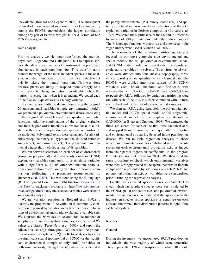
The remainder of the variation partitioning analysesfocused on our most comprehensive environmental andspatial models, the full polynomial environmental modeland PCNM spatial model. We Wrst divided the signiWcantexplanatory variables into subsets. The environmental vari-ables were divided into four subsets: topography, foreststructure, soil type, and quantitative soil chemical data. ThePCNMs were divided into three subsets of 34 PCNMvariables each: broad-, medium- and Wne-scale, withwavelengths c. 100–300, 300–650 and 650–2,000 m,respectively. RDAs followed by variation partitioning wererun with each of the PCNM subsets combined with, in turn,each subset and the full set of environmental variables.
We then ran RDA using separately the polynomial spa-tial model, full PCNM spatial model or full polynomialenvironmental model as the explanatory dataset inCANOCO (ter Braak and Smilauer 1998). We extracted theWtted site scores for each of the Wrst three canonical axesand mapped them, to visualize the major patterns of spatialand environmental structuring detected in the pteridophytedataset. We ran multiple regression analyses to checkwhich environmental variables contributed most to the sitescores on each environmental ordination axis, as judgedfrom their partial regression coeYcients, in the programPermute (version 3.4, Casgrain 2001). We then used thesame procedure to check which environmental variableswere most strongly related to the spatial patterns in Xoristiccomposition represented by site scores on each PCNM andpolynomial ordination axis. All variables were standardizedprior to running the regression analyses.
Finally, we extracted species scores in CANOCO tocheck which pteridophyte species were best modelled bythe PCNM spatial ordination axes and polynomial environ-mental ordination axes. We tabulated the species with thehighest ten species scores (positive or negative) on eachaxis and interpreted their distribution patterns in light of theexplanatory data.
Results
General
During the inventory, we encountered 89,708 pteridophyteindividuals, the vast majority of which were terrestrial.They represented 128 morphospecies, of which 103 could
123

Oecologia (2008) 155:593–604 597
be identiWed to a named species, 24 were identiWed to genuslevel, and one (a single plant) remained unidentiWed. Twoof the named species were confused in the Weld and arecombined in the analyses, which hence include 127 species.Each 100-m2 plot contained from three to 780 pteridophyteindividuals (mean 86, median 72) and from one to 28 spe-cies (mean 10, median 9). The most abundant species wasrepresented by 25,439 individuals in the entire dataset, andthe least abundant 11 species were represented by a singleindividual each (mean 706, median 41). The Wve mostabundant species, in descending order of abundance, wereDanaea wendlandii, Salpichlaena sp. 1, Polybotrya villo-sula, Lomariopsis vestita and Adiantum obliquum (seeTable 1 for authorities).
Variation partitioning
Forward selection included all 20 original environmentalvariables as signiWcant predictors of variation in commu-nity composition in the simple environmental model, and39 of 48 terms in the polynomial environmental model. Thesimple environmental model explained Ra
2 =21.0% ofcommunity variation and the polynomial environmentalmodel explained 25.8%. In the latter case, total variationexplainable using soil chemistry was 19.1%, followed bytopography (14.3%), soil type (8.9%) and forest structure(3.5%). These subsets of environmental data were partlyredundant (Fig. 1), but each also made a unique contribu-tion to explained variation. The unique contribution of soil
chemistry was the largest (7.1%), followed by topography(4.1%), forest structure (1.1%), and soil type (1.0%).
Forward selection of the spatial variables included allnine terms of the polynomial spatial model, and 102 of 665PCNMs in the PCNM spatial model. The polynomial spa-tial model explained 4.3% of the variation in pteridophytecommunity composition and the PCNM spatial modelexplained 15.9%.
Depending on the combination of spatial and environ-mental models used, the variation partitioning results variedgreatly (Fig. 2). The lowest total variation explained(TVE), 6.9%, resulted when the polynomial spatial modelwas combined with the simple model of forest structure.The highest TVE (32.3%) resulted when the PCNM spatialmodel was combined with the polynomial model of allenvironmental data. Similarly, the PE fraction varied from1.8 to 23.7%, the SSE fraction from 0.3 to 9.4%, and the PSfraction from 2.2 to 14.8%. When the polynomial spatialmodel was used, PE > PS resulted in all cases except whenthe environmental model comprised forest structural dataalone. When the PCNM spatial model was used, the situa-tion was usually reversed, but PE > PS resulted both whenall environmental data types were used, and when soilchemical variables were used together with their polynomi-als (Fig. 2).
We further decomposed the PS and the SSE fractions ofvariation explained by our most comprehensive model intobroad, medium and Wne-scale fractions. Most of the spatialstructure in community composition was found at broad
Table 1 Pteridophyte species with the clearest relationships (ten high-est species scores) with each of the Wrst three constrained RDA axes.The explanatory variables consisted of either a spatial model based onprincipal coordinates of neighbour matrices (PCNM) or an environ-
mental model based on all available environmental variables and theirpolynomials. Positive (+) and negative (¡) species scores are shownseparately; within each category, the species are listed in order ofdecreasing absolute value of their scores
PCNM axis 1 PCNM axis 2 PCNM axis 3 Env. axis 1 Env. axis 2 Env. axis 3
+ Trich coll + Thely nica + Lomar vest + Thely nica + Polyb vill + Lomar vest
+ Polyb osmu + Trich coll + Polyb vill + Trich coll + Thely nica + Polyt feei
+ Thely nica + Campy sphe + Asple cirr + Tecta athy/riva + Sacco inae + Trich coll
+ Lomar vest + Tecta athy/riva + Polyp lori + Salpi sp1
+ Selag arth + Selag arth + Bolbi nico + Dipla stri
+ Tecta athy/riva + Dipla stri + Dipla stri
+ Bolbi nico
+ Tecta sp7
+ Pteris sp2
¡ Polyb vill ¡ Danae wend ¡ Polyb alfr ¡ Adian obli ¡ Danae wend ¡ Polyp lori
¡ Salpi sp1 ¡ Polyp lori ¡ Polyb vill ¡ Lomar vest ¡ Trich eleg
¡ Adian obli ¡ Polyb osmu ¡ Sacco inae ¡ Asple cirr ¡ Danae medi
¡ Sacco inae ¡ Elaph sp9 ¡ Salpi sp1 ¡ Trich eleg ¡ Cyath ursi
¡ Salpi sp1 ¡ Alsop cusp ¡ Elaph sp9
¡ Trich eleg ¡ Alsop cusp
¡ Tecta plan ¡ Polyb alfr
123

598 Oecologia (2008) 155:593–604
spatial scales (>650 m) in both the PS and SSE fractions.Environmental variables contributed slightly more at Wne(100–300 m) than at medium scales, with the exception ofsoil type (Fig. 2d).
Spatio-environmental patterns in pteridophyte community composition
In the RDA analysis where polynomial environmental datawere used as explanatory variables, the Wve environmentalvariables with the largest partial contributions to axis 1(henceforth environmental axis 1) were (soil Mg)2, soil Ca,slope, topographic position, and soil pH. This axis can beinterpreted as a Xoristic gradient from Xat, relatively fertileswamp and other poorly drained sites at low topographicpositions to sloping, relatively poor, well-drained sites athigher topographic positions (Fig. 3). Environmental axes 2and 3, in contrast, reXect Xoristic variation independent ofthis swamp–upland gradient. Environmental axis 2 is inter-pretable as Xoristic responses to relatively Wne-scale varia-tion in exchangeable cations and topography, andenvironmental axis 3 reXects responses to variation in soilorganic matter, especially between stream valleys and othersites. The Wve variables with the largest partial contribu-tions to environmental axis 2 were (soil Ca)2, (soil Ca)3,(soil Mg)2, (soil pH)2 and (soil P)3. Topographic positionalso made a sizeable contribution to this axis, ranking sixth.The Wve variables with the largest partial contributions to
environmental axis 3 were soil C, soil N, (soil C)2, slopeand soil Ca. Canopy openness also made a relatively largecontribution to this axis, ranking seventh. Generally, how-ever, the contributions of the soil type and forest structuralvariables to all three environmental axes were minor.
In the RDA analysis where PCNM spatial data wereused as explanatory variables, axis 1 (henceforth PCNMaxis 1) clearly separated the largest swamp with its
Fig. 1 Partitioning of the variation in pteridophyte community com-position using four subsets of environmental data: soil type (S), soilchemistry (C), forest structure (F) and topography (T). The enclosingbox indicates total variation in composition, of which 25.8% was ex-plained by the environmental datasets. The rectangles within the boxapproximately indicate the fraction of explained variation attributableto each environmental dataset (forest structure is divided into two sep-arate rectangles to allow its illustration). The exact sizes of the uniquecontributions of each dataset, as well as their intersections, are listed tothe right of the Wgure. All the testable model fractions (i.e. the uniquecontributions) were signiWcant with P = 0.001 after 999 permutations
Fig. 2 Variation in pteridophyte community composition explainedusing two diVerent spatial models based on the x and y coordinates ofthe plots [a third-order polynomial (a, b) or principal coordinates ofneighbour matrices (PCNM) variables (c, d)], and ten diVerent envi-ronmental models (Wve categories of environmental data and two lev-els of model complexity). The environmental data categories were alldata (All), soil chemistry alone (C), topography alone (T), soil typealone (S) and forest structure alone (F). Environmental model com-plexity refers to either a simple model of the selected environmentalvariables (a, c) or to a polynomial model including cubic and quadraticfunctions of the selected variables as well (b, d). For every spatial andenvironmental model combination, explained variation is partitionedinto three fractions: purely spatial (space), spatially structured environ-mental (space + environment) and purely environmental (environ-ment). For the most comprehensive model (d), the spatial and spatiallystructured environmental fractions of explained variation are furtherpartitioned by spatial scale (from top to bottom: broad, medium, Wne).All the testable model fractions (i.e. purely spatial or purely environ-mental fractions) were signiWcant with P = 0.001 after 999 permuta-tions
123
Oecologia (2008) 155:593–604 599
surroundings and some stream valleys both from manyupland areas and from the two smaller swamps, one ofwhich was largely treeless (Fig. 3). PCNM axis 2 was visi-bly similar to environmental axis 1, and also mainly reX-ected the gradient from poorly drained soils to uplands,whereas PCNM axis 3 was less environmentally interpret-able, although it showed some correspondence with envi-ronmental axis 3 (Fig. 3). Although environmental
variables were not included in the analysis, there was astrong positive relationship between site scores on PCNMaxes 1 and 3 and the swamp soil type and soil Ca concentra-tion, respectively, and a strong negative relationshipbetween site scores on PCNM axis 2 and the residual soiltype (all P < 0.001 in multiple regression analysis).
In the RDA analysis where polynomial spatial data wereused as explanatory variables, site scores on axis 1 (hence-
Fig. 3 Distributions across the study site at La Selva Biological Station of a soil types, b eleva-tion classes and c–k site scores of 100 m2 pteridophyte sampling plots on the ordination axes 1–3 obtained in redundancy analy-ses. Site scores were obtained using as the explanatory dataset either the polynomial environ-mental (Poly. Envir.) model (c–e), the PCNM spatial model (f–h) or the polynomial spatial (Poly. Spatial) model (i–k). The Wlled circles indicate positive values, and the open circles negative values. The site scores represent the main gradients detected in species composition, as predicted by a linear combina-tion of the explanatory variables. The proportion of variation in species composition explained by each axis (Ra
2 ) is given in parentheses
123

600 Oecologia (2008) 155:593–604
forth polynomial axis 1) showed a much coarser spatial pat-tern that resembled that of environmental axis 1 and PCNMaxes 1 and 2 (Fig. 3). Among the environmental variables,soil Ca was most strongly and positively related to sitescores on polynomial axis 1, the residual soil type nega-tively to scores on polynomial axis 2, and soil P positivelyto scores on polynomial axis 3 (all P < 0.001).
Recording the ten species with the highest species scoreson each of the environmental and PCNM axes produced alist of 26 species, of which 19 had high scores along morethan one axis (Table 1). For eight species (e.g. Polybotryavillosula, Danaea wendlandii and Thelypteris nicaraguen-sis; Fig. 4), observed spatio-environmental distribution pat-terns seem to represent a primary relationship with theswamp to non-swamp gradient (environmental axis 1 orPCNM axis 2), and a secondary relationship with edaphic–topographic variation in non-swamp areas (environmentalaxis 2 or 3; Table 1). Four species (e.g. Trichomanes col-lariatum; Fig. 4), had spatial distribution patterns stronglyreXected in both PCNM axes 1 and 2 (Table 1), which indi-cates a main distributional bias either towards or away fromthe largest, forested swamp and its surroundings, and a sec-ondary bias related to swamp soils more generally. Thespatial distributions of four species (e.g. Polybotrya villo-sula, Polybotrya osmundacea and Lomariopsis vestita;Fig. 4), were strongly reXected in PCNM axis 1 and sec-ondarily in PCNM axis 3 (Table 1). The distributions of afurther suite of species did not indicate any strong biasalong the swamp–upland gradient, but these were insteadassociated with stream and other humid valleys (e.g.Polypodium loriciforme, with a relatively high speciesscore on both environmental axis 3 and PCNM axis 3;Fig. 4, Table 1).
Many species pairs had complementary distribution pat-terns, often resulting from biases either towards or awayfrom swamp-like conditions (e.g. Thelypteris nicaraguensis
vs. Danaea wendlandii; Fig. 4). The three Polybotrya spe-cies also had notably contrasting distributions. Polybotryavillosula contrasted with Polybotrya osmundacea alongPCNM axis 1 (highly negative vs. positive species scores,respectively), and with Polybotrya alfredii along PCNMaxis 3 (highly positive vs. negative species scores, respec-tively). Whereas Polybotrya villosula had high speciesscores on environmental axes 1 and 2, Polybotrya alfrediihad a high species score on environmental axis 3 (Fig. 4,Table 1).
Discussion
Ecological interpretation of community variability
With the variables at hand, we were able to explain up to32% of pteridophyte community variation (after correctingfor sample size and the number of explanatory variables;Peres-Neto et al. 2006). The main axes of Xoristic diVeren-tiation could roughly be characterized as diVerencesbetween swamps and uplands, between open and forestedswamps, between ridge tops and valleys, and between sitesvarying in their organic matter deposition and proximity tostreams. Especially soil pH, soil concentrations of Ca, Mg,C and N, and slope angle and relative topographic positionwere strongly related to these major axes of Xoristic varia-tion. The distributions of numerous pteridophyte speciesreXected more than one of these gradients. Soil Ca and Mgcontents have been identiWed as important in several earlierstudies of pteridophyte communities in Amazonian forests,at spatial scales ranging from metres to kilometres (e.g.Tuomisto et al. 2003a; Costa et al. 2005; Poulsen et al.2006). Topographic variation was another major factor bothin these studies and in a recent temperate forest study at asimilar scale to ours (Karst et al. 2005). Responses to soil
Fig. 4 a–h Distribution maps of the eight pteridophyte species discussed in the text. Small dots represent the locations of 100-m2 study plots at La Selva Bio-logical Station. Larger circles indicate presence of the species in question, with the size of the circle proportional to the Hellin-ger-transformed abundance of the species
123

Oecologia (2008) 155:593–604 601
pH have often been less apparent (except in Karst et al.2005) than at our site, where pH variation is strongly linkedwith the main swamp–upland gradient and exchangeablecation contents. When soil C and N (or NO3
¡) concentra-tions have been investigated, they have also been foundimportant for explaining fern distributions (Costa et al.2005; Karst et al. 2005).
The pteridophyte species whose distributions were moststrongly related to the RDA axes diVered widely in theirrelationships with environmental variables. Many specieshad contrasting distributions, which in some cases clearlyreXected speciWc environmental variables (e.g. Thelypterisnicaraguensis and Danaea wendlandii showed oppositeassociations with swamp and upland soils). In other casesthe relationships were less obvious. For example, the rarePolybotrya alfredii was restricted to a single valley,whereas congeneric Polybotrya villosula and Polybotryaosmundacea were abundant but mutually negatively associ-ated elsewhere. The distribution of Polybotrya villosulashowed strong environmental structuring, but that of Polyb-otrya osmundacea did not. Without information about thedistributions of these species over time, and over broaderspatial scales and longer ecological gradients (cf. Tuomisto2006), it is diYcult to draw conclusions about the relativeroles of niche diVerentiation and other factors in determin-ing these patterns.
Spatial structure in community composition was evidentat all scales encompassed by our study design. The environ-mental component to spatially explained variation in com-munity composition was strongest at broad scales (650–2,000 m), but was stronger at Wne (100–350 m) than atintermediate scales. This pattern probably reXects the spa-tial conWguration of environmental conditions at our site.Much of the broad-scale spatial variability is attributable toXoristic diVerences between the largest swamp and otherareas. The detected Wne-scale spatial variability is morelikely related to diVerences in soil fertility, drainage, and airhumidity along topographic gradients.
The complex and varied patterns of Xoristic variationidentiWed here, and the fact that these were strongly associ-ated with quantitative variation in soil chemistry, suggestthat habitat speciWcity in this community would be severelyunderestimated if habitat were characterized by soil type ortopographic position alone, as has often been done in rainforest studies (Harms et al. 2001; Cannon and Leighton2004; Valencia et al. 2004; but see Hall et al. 2004; Johnet al. 2007). By extension, fewer rain forest species may behabitat generalists than earlier studies have proposed.
The purely spatial fraction of explained variation hassometimes been interpreted as predominantly a dispersaleVect (e.g. Gilbert and Lechowicz 2004; Cottenie 2005;Karst et al. 2005), but we do not believe this to be the casein our study. We suspect that this fraction had a consider-
able environmental component, which was not detectedbecause some relevant environmental variables were omit-ted even from our most comprehensive dataset. For exam-ple, the main spatial pattern detected in our Xoristic datacorresponded to the distinction between forested swampconditions as opposed to open swamp and uplands, but thiswas not well captured by our environmental data. Temporalvariation in environmental conditions, caused by gapdynamics or climatic variability, may also produce a spatialpattern that a snap shot environmental dataset cannot repre-sent.
A relatively large proportion (at least 68%) of commu-nity variation in our dataset was unexplained by either envi-ronmental or spatial data. Undoubtedly, this is partly due torandom spore dispersal and mortality, but it may alsoinclude deterministic variation caused by unmeasured envi-ronmental variables. Moreover, the role of processes oper-ating at Wner scales than those covered by a study’ssampling design cannot be quantiWed. These may be veryimportant at our site, as strong turnover in pteridophytespecies composition has been identiWed at distances lessbelow 100 m (Jones et al. 2006). Some local turnover isvisibly related to environmental variation, but distance-lim-ited spore dispersal and interspeciWc interactions are alsolikely to be strongest at short distances.
Data quality and variation partitioning
We obtained very diVerent variation partitioning resultsdepending on which of 20 alternative combinations of envi-ronmental and spatial data we used as explanatory vari-ables. The total proportion of explained Xoristic variationvaried more than fourfold, as did the proportion explainedby space, and the proportion explained by the environmentvaried ninefold. The unique contribution of the environ-ment varied 12-fold, and the unique contribution of spaceWvefold. When the results are interpreted in terms of the rel-ative importance of space versus environment, the ratio ofthe PS to PE fractions is of particular interest. This ratioranged from 1:11 to 8:1 (or excluding the forest structuralmodel, which was our most poorly performing environmen-tal model, from 1:11 to 3:1). This shows that the main resultof a study can easily be reversed by model choice.
Given that the variation partitioning method is an exten-sion of multiple regression, diVerent explanatory modelscan be expected to give somewhat diVerent results. How-ever, the magnitude of this eVect has been underestimatedor overlooked in recent comparisons (e.g. Balvanera et al.2002; Cottenie 2005; Chust et al. 2006).
We found that over two-thirds of the spatial Xoristic var-iation detected by the PCNM model was undetected by thepolynomial model. Of the four environmental data types,soil chemical data had the highest power to explain Xoristic
123

602 Oecologia (2008) 155:593–604
variation, followed by topographic, soil type and foreststructural descriptors. Although these environmental datatypes were partly redundant, total environmentally explain-able variation would have been reduced by a third if hadsoil chemistry been omitted from our study.
How do these results compare with earlier Xoristic varia-tion partitioning studies? Most studies where spaceexplained more variation than environment used no data onsoil chemistry (Borcard et al. 1992; Svenning et al. 2004 fortrees; Chust et al. 2006). Svenning and Skov (2005) providean exception, but their data were derived from coarse-scalemaps rather than actual soil sampling. In contrast, in thosestudies where environment explained more variation thanspace, either soil chemical data were included (Duivenvoor-den 1995; Gilbert and Lechowicz 2004; Duque et al. 2005;Karst et al. 2005; possibly Cottenie 2005 in some cases),disturbed landscapes were included (Dalle et al. 2002), orthe spatial model was especially coarse (Duivenvoorden1995; Balvanera et al. 2002). In these cases, model choiceseems to be a strong predictor of the analysis results.
Austin (2002) suggested that canonical ordination analy-ses would yield ecologically more meaningful results byenabling non-linear functions of environmental variables.In the present study, which covered a limited range of eco-logical variation, including polynomials of the environmen-tal variables increased total environmentally explainedvariation by between one-quarter and one-third. In broaderscale studies that encompass a wider range of environmen-tal conditions, the results of linear and non-linear methodscan be expected to diverge much more.
In addition to diVering in their explanatory variables,community studies have also diVered in their response vari-able (species presence–absence or abundance data, focaltaxa), in the ordination method applied (RDA or CCA), andin spatial extent, spatial resolution, and the environmentalgradients they cover. The overall proportion of explainedvariation should be adjusted for the number of samplingsites and explanatory variables (Legendre et al. 2005;Peres-Neto et al. 2006), but this adjustment has yet to becommonly implemented. Consequently, it is almost impos-sible to evaluate to what degree diVerences in the resultsamong studies are methodological, and to what degree theyreXect real diVerences among focal plant groups or geo-graphical areas. Studies applying consistent methods incross-site and cross-taxon analyses would be of particularvalue for resolving these issues.
Conclusion
We found evidence of strong environmental control ofbeta-diversity in Costa Rican rain forest pteridophytes.However, the explanatory power of environmental and spa-tial variables together varied between 7 and 32%, and the
relative importance of “space” and “environment” could bereversed by model choice. This leads us to the followingconclusions about the interpretation of variation partition-ing results, and recommendations for future studies:
1. Ecological background knowledge is needed whenselecting environmental variables to avoid omittingkey factors. Plant growth is known to depend on theavailability of various nutrients, water and light, soquantitative descriptors of these should be included inXoristic studies. Incorporating non-linear relationshipsbetween Xoristic and environmental variation may alsobe needed, especially if the sampled environmentalgradient is long. Results cannot be assumed to reXectthe eVect of “the environment” in general, unless allpotentially relevant environmental variables have beenadequately modelled.
2. For the adequate modelling of “space”, a suYcientlyXexible spatial model is needed. A simple spatialmodel, such as one based on x and y coordinates, orpolynomial functions of these, will only be able to rep-resent broad-scale spatial patterns. The ability to detectspatial pattern will also depend on the sampling setup,such as interplot distances and the spatial arrangementof the plots.
3. R2 adjustment needs to be applied to eliminate theinXuence of sample size and the number of explanatoryvariables on the proportion of variation explained.
4. Great care needs to be taken in interpreting the results,as these are subject to constraints imposed by the data-set and the methods applied. Both generalisations froma particular study and comparisons across studies needto carefully consider these constraints. Biologicalmeaning can only be separated from methodologicalartefacts if the impact of data quality on the results isrecognised.
Acknowledgements We thank Rigoberto Gonzalez for assistingduring the fern inventory, and Jens Mackensen and Edzo Veldkamp forsoil data collection. Diana and Milton Lieberman kindly allowed us ac-cess to their study areas. La Selva Biological Station of the Organiza-tion for Tropical Studies provided logistic support. Jérôme Chave,Michael Kessler and three anonymous reviewers provided helpfulcomments on the manuscript. The work was funded by grants from theAcademy of Finland (to H. Tuomisto), the Andrew W. Mellon founda-tion (to D. B. and D. A. Clark), and NSERC (grant numberOGP0007738 to P. Legendre). Inventories and specimen collectioncomplied with Costa Rican law. Research permits were kindly grantedby SINAC-MINAE.
References
Arbeláez MV, Duivenvoorden JF (2004) Patterns of plant species com-position on Amazonian sandstone outcrops in Colombia. J VegSci 15:181–188
123

Oecologia (2008) 155:593–604 603
Austin MP (2002) Spatial prediction of species distribution: an inter-face between ecological theory and statistical modelling. EcolModell 157:101–118
Balvanera P, Lott E, Segura G, Siebe C, Islas A (2002) Patterns of �-diversity in a Mexican tropical dry forest. J Veg Sci 13:145–158
Blanchet G, Legendre P, Borcard D (2007) Forward selection ofexplanatory variables. Ecology (in press)
Borcard D, Legendre P (2002) All-scale spatial analysis of ecologicaldata by means of principal coordinates of neighbour matrices.Ecol Modell 153:51–68
Borcard D, Legendre P (2004) SpaceMaker2––user’s guide. Départe-ment de sciences biologiques, Université de Montréal. http://www.bio.umontreal.ca/legendre/
Borcard D, Legendre P, Avois-Jacquet C, Tuomisto H (2004) Dissect-ing the spatial structure of ecological data at multiple scales. Ecol-ogy 85:1826–1832
Borcard D, Legendre P, Drapeau P (1992) Partialling out the spatialcomponent of ecological variation. Ecology 73:1045–1055
ter Braak CJF, Smilauer P (1998) CANOCO reference manual and us-er’s guide to CANOCO for Windows. Software for canonical com-munity ordination. Version 4. Centre for Biometry, Wageningen
Brown N, Jennings S, Wheeler P, Nabe-Nielsen J (2000) An improvedmethod for the rapid assessment of forest understorey light envi-ronments. J Appl Ecol 37:1044–1053
Cannon CH, Leighton M (2004) Tree species distributions across Wvehabitats in a Bornean rain forest. J Veg Sci 15:257–266
Casgrain P (2001) Permute! Version 3.4 user’s manual. Départementde sciences biologiques, Université de Montréal, Montreal
Chust G, Chave J, Condit R, Aguilar S, Lao S, Pérez R (2006) Deter-minants and spatial modeling of tree �-diversity in a tropical for-est landscape in Panama. J Veg Sci 17:83–92
Clark DA, Clark DB, Sandoval M R, Castro C MV (1995) Edaphic andhuman eVects on landscape-scale distributions of tropical rain for-est palms. Ecology 76:2581–2594
Clark DB, Palmer MW, Clark DA (1999) Edaphic factors and the land-scape-scale distributions of tropical rain forest trees. Ecology80:2662–2675
Corney PM, Le Duc MG, Smart SM, Kirby KJ, Bunce RGH, Marrs RH(2006) Relationships between the species composition of forestWeld-layer vegetation and environmental drivers assessed using anational scale survey. J Ecol 94:383–401
Cottenie K (2005) Integrating environmental and spatial processes inecological community dynamics. Ecol Lett 8:1175–1182
Dalle SP, López H, Díaz D, Legendre P, Potvin C (2002) Spatial dis-tribution and habitats of useful plants:an initial assessment forconservation on an indigenous territory Panama. Biodivers Con-serv 11:637–667
Dalling JW, Muller-Landau HC, Wright SJ, Hubbell SP (2002) Role ofdispersal in the recruitment limitation of neotropical pioneer spe-cies. J Ecol 90:714–727
Denslow JS (1987) Tropical rainforest gaps and tree species diversity.Annu Rev Ecol Syst 18:431–451
Dirzo R, Horvitz CC, Quevedo H, López MA (1992) The eVects of gapsize and age on the understorey herb community of a tropicalMexican rain forest. J Ecol 80:809–822
Dray S, Legendre P, Peres-Neto PR (2006) Spatial modelling: a com-prehensive framework for principal coordinate analysis of neigh-bour matrices (PCNM). Ecol Modell 196:483–493
Duivenvoorden JF (1995) Tree species composition and rain forest-environment relationships in the middle Caquetá area ColombiaNW Amazonia. Vegetatio 120:91–113
Duque A, Sánchez M, Cavallier J, Duivenvoorden JF (2002) DiVerentXoristic patterns of woody understorey and canopy plants inColombian Amazonia. J Trop Ecol 18:499–525
Duque AJ, Duivenvoorden JF, Cavelier J, Sanchez M, Polanía C, LeónA (2005) Ferns and Melastomataceae as indicators of vascular
plant composition in rain forests of Colombian Amazonia. PlantEcol 178:1–13
Fine PVA, Mesones I, Coley PD (2004) Herbivores promote habitatspecialization by trees in Amazonian forests. Science 305:663–665
Gilbert B, Lechowicz MJ (2004) Neutrality niches and dispersal in atemperate forest understory. Proc Natl Acad Sci USA 101:7651–7656
Hall JS, McKenna JJ, Ashton PMS, Gregoire TG (2004) Habitat char-acterizations underestimate the role of edaphic factors controllingthe distribution of Entandrophragma. Ecology 85:2171–2183
Harms KE, Condit R, Hubbell SP, Foster RB (2001) Habitat associa-tions of trees and shrubs in a 50-ha neotropical forest plot. J Ecol89:947–959
Hofton MA, Rocchio LE, Blair JB, Dubayah R (2002) Validation ofVegetation Canopy Lidar sub-canopy topography measurementsfor a dense tropical forest. J Geodyn 34:491–502
Holmgren PK, Holmgren NH (1998 onwards) [continuously updated].Index Herbariorum. New York Botanical Garden. http://sci-web.nybg.org/science2/IndexHerbariorum.asp
Hubbell SP (2001) The uniWed neutral theory of biodiversity and bio-geography. Princeton University Press, Princeton
John R, Dalling JW, Harms KE, Yavitt JB, Stallard RF, Mirabello M,Hubbell SP, Valencia R, Navarrete H, Vallejo M, Foster RB(2007) Soil nutrients inXuence spatial distributions of tropical treespecies. Proc Natl Acad Sci USA 104:864–869
Jones MM, Tuomisto H, Clark DB, Olivas P (2006) EVects of meso-scale environmental heterogeneity and dispersal limitation on Xo-ristic variation in rain forest ferns. J Ecol 94:181–195
Karst J, Gilbert B, Lechowicz MJ (2005) Fern community assembly:the roles of chance and the environment at local and intermediatescales. Ecology 86:2473–2486
Legendre P, Gallagher ED (2001) Ecologically meaningful transfor-mations for ordination of species data. Oecologia 129:271–280
Legendre P, Borcard D, Peres-Neto PR (2005) Analyzing beta diver-sity: partitioning the spatial variation of community compositiondata. Ecol Monogr 74:435–450
Moran RC, Riba R (eds) (1995) Flora Mesoamericana, vol 1. Psilota-ceae a Salviniaceae. Universidad Nacional Autónoma de México,Mexico
Oksanen J, Kindt R, Legendre P, O’Hara RB (2007) vegan: communityecology package version 1.8–5. http://cc.oulu.W/»jarioksa/
Peres-Neto PR, Legendre P, Dray S, Borcard D (2006) Variation par-titioning of species data matrices: estimation and comparison offractions. Ecology 87:2614–2625
Phillips OL, Núñez Vargas P, Lorenzo Monteagudo A, Peña Cruz A,Chuspe Zans M-E, Galiano Sánchez W, Yli-Halla M, Rose S(2003) Habitat association among Amazonian tree species: alandscape-scale approach. J Ecol 91:757–775
Potts MD, Ashton PS, Kaufman LS, Plotkin JB (2002) Habitat patternsin tropical rain forests: a comparison of 105 plots in northwestBorneo. Ecology 83:2782–2797
Poulsen AD, Tuomisto H, Balslev H (2006) Edaphic and Xoristic var-iation within a 1-ha plot of lowland Amazonian rain forest. Bio-tropica 38:468–478
R Development Core Team (2006) R: A language and environment forstatistical computing. R Foundation for Statistical Computing,Vienna, ISBN 3–900051-07-0, http://www.R-project.org
Svenning J-C, Kinner DA, Stallard RF, Engelbrecht BMJ, Wright SJ(2004) Ecological determinism in plant community structureacross a tropical forest landscape. Ecology 85:2526–2538
Svenning J-C, Skov F (2005) The relative roles of environment andhistory as controls of tree species composition and richness in Eu-rope. J Biogeogr 32:1019–1033
Thomsen RP, Svenning J-C, Balslev H (2005) Overstorey control ofunderstorey species composition in a near-natural temperatebroadleaved forest in Denmark. Plant Ecol 181:113–126
123

604 Oecologia (2008) 155:593–604
Tuomisto H (2006) Edaphic niche diVerentiation among Polybotryaferns in Western Amazonia: implications for coexistence and spe-ciation. Ecography 29:273–284
Tuomisto H, Poulsen AD (2000) Pteridophyte diversity and speciescomposition in four Amazonian rain forests. J Veg Sci 11:383–396
Tuomisto H, Ruokolainen K, Kalliola R, Linna A, Danjoy W, Rodri-guez Z (1995) Dissecting Amazonian biodiversity. Science269:63–66
Tuomisto H, Poulsen AD, Ruokolainen K, Moran RC, Quintana C,Celi J, Cañas G (2003a) Linking Xoristic patterns with soil heter-ogeneity and satellite imagery in Ecuadorian Amazonia. EcolAppl 13:352–371
Tuomisto H, Ruokolainen K, Yli-Halla M (2003b) Dispersal environ-ment and Xoristic variation of Western Amazonian forests. Sci-ence 299:241–244
Valencia R, Foster RB, Villa G, Condit R, Svenning J-C, Hernández C,Romoleroux K, Losos E, Magård E, Balslev H (2004) Tree spe-cies distributions and local habitat variation in the Amazon: largeforest plot in eastern Ecuador. J Ecol 92:214–229
Vormisto J, Svenning J-C, Hall P, Balslev H (2004) Diversity anddominance in palm (Arecaceae) communities in terra Wrme for-ests in the western Amazon basin. J Ecol 92:577–588
Wyatt JL, Silman MR (2004) Distance-dependence in two Amazonianpalms: eVects of spatial and temporal variation in seed predatorcommunities. Oecologia 140:26–35
123