explaining the low labor productivity in east germany ... · explaining the low labor productivity...

Explaining the

Low Labor Productivity in East Germany -

A Spatial Analysis

Nicola Fuchs-Schündeln and Rima Izem∗

September 28, 2009

Abstract

This paper sheds light on the transferability of human capital in periods of dramatic

structural change by analyzing the unique event of German Reunification. We explore

whether the comparatively low labor productivity in East Germany after reunification

is caused by the depreciation of human capital at reunification, or by unfavorable job

characteristics. East German workers should have been hit harder by reunification the

more specific human capital was. Treating both human capital and job characteristics

as unobservables, we derive their relative importance in explaining the low labor pro-

ductivity by estimating a spatial structural model that predicts commuting behavior

across the former East-West border and the resulting regional unemployment rates.

The identification of the model is based on the slope of the unemployment rate across

the former border: the larger the human capital differences between East and West,

the less commuting across the border takes place, and the sharper is the increase of

the unemployment rate at the former border. The results indicate that East and West

German skills are very similar, while job characteristics differ significantly between East

and West. Hence, they suggest that a significant part of the human capital accumulated

in the East before 1990 was transferable. (JEL: C15, J24, J61; keywords: transferability

of human capital, spatial allocation of labor)

1 Introduction

German reunification provides a unique opportunity to study the transferability of human

capital in a period of severe structural changes. According to traditional measures of hu-

man capital, like years of schooling or further education, the East German population was

better educated at reunification than was the West German population. If human capital

is very general and transferable, e.g. mostly consisting of general problem-solving, lan-

guage or mathematical skills, the East German population should have fared very well in

∗We thank Guido Imbens, Matthias Schündeln, Harald Uhlig, and the seminar audiences at various placesfor their feedback and suggestions. We thank Susanne Raessler and Katja Wolf from the IAB for wonderful

hosting in Nuremberg, and for all their help and feedback with the data; and Anders Hopperstedt from the

Center of Geographic Analysis at Harvard for calculating the driving times between counties. Kirk Moore,

Kelly Shue, Andreas Fuster, Carolin Pflueger and Linjuan Qian provided excellent research assistantship.

This research was partly funded by the William Milton Fund and a research grant by the Wheatherhead

Center for International Affairs at Harvard University.

1

the new West German labor market. However, the content of education and on the job

training might have differed substantially between both countries, and a lot of either job-,

industry-, occupation-, or technology-specific human capital should thus have depreciated

at reunification.1

The analysis of this paper answers questions of broad policy importance. How easily is

human capital transferred from an obsolete industry to the next? What is the relationship

between depressed and booming regions? German reunification provides a unique oppor-

tunity to study these questions. In contrast to other possible case studies, e.g. the car

industry in Michigan, or a comparison of Northern and Southern Italy, the German case

offers three unique advantages: First and foremost, there exists a clearly defined “border”

between the two regions in question, namely the former border between East and West

Germany. Second, there is a clear point in time at which we would expect human capital of

one region to depreciate if it were specific to the job, occupation, industry, or technology,

namely German Reunification in 1990. Last, these two regions offer a very stark contrast.

German reunification rendered many East German technologies obsolete. Within four years

of reunification, the government only managed to sell around two-thirds of all East German

government-owned firms, despite the creation of a special agency in charge of the priva-

tization. Of the privatized firms, around half were liquidated by 1994 anyhow (Grosser,

2003).2

Since German reunification in 1990, unemployment rates in East Germany have been

stubbornly high. Figure 1 shows the mean unemployment rates by county (Kreis) between

1998 and 2004, as well as the former East-West border. There are 439 counties in Germany,

of which 326 belong to the former West.3 The average population size of a county is 188,000.

Unemployment rates are calculated as the ratio of people registered as unemployed to the

sum of all employees and unemployed.4 On average, unemployment rates in the East are

around twice as high as those in the West.

By now, it is well established that the major cause of the high unemployment rates

in the East lies in wages exceeding labor productivity (see e.g. Burda and Hunt, 2001).

Figure 2 shows the East-West ratios of wages in addition to the East-West ratios of labor

1The distinction between general skills and skills specific to a firm or occupation dates back at least to

Becker (1964) and Mincer (1974). Chari and Hopenhayn, 1991, and Violante, 2002, analyze the effect of

vintage specific human capital on the diffusion of new technologies and wage inequality, respectively.2The government-owned firms originally provided 4.1 million jobs, while the total population in the East

amounted to 17 million people. In 1994, the privatized firms only provided 1.5 million jobs.3During our sample period 1998 to 2004, there was one county reform, involving Hannover. From 2002

on, Hannover is one county, while before it was split into Stadtkreis and Landkreis Hannover. We treat

Hannover as one county throughout, and sum up or build averages over Stadtkreis and Landkreis data for

1998 to 2001, as appropriate.4This sum includes in addition to the unemployed employees subject to mandatory social insurance

contributions, part-time employees, and civil servants, but excludes self-employed, for whom only estimates

exist on the county level.

2

Figure 1: Mean Unemployment Rates in German Counties, 1998 to 2004

3

0

0.1

0.2

0.3

0.4

0.5

0.6

0.7

0.8

0.9

1

1991

1992

1993

1994

1995

1996

1997

1998

1999

2000

2001

2002

2003

2004

wages

GDP per employee

Figure 2: East-West ratios of wages and labor productivity, 1991 to 2004

productivity, measured as GDP per employee, from 1991 to 2004. The trend in both ratios

has been remarkably similar. There is rapid convergence between East and West until 1995,

and from then on convergence has slowed down significantly, or even come to a halt. Most

importantly, the East-West ratio of wages is always larger than the East-West ratio of labor

productivity, and there is only a small and slow decline in the difference between both.

Thus, it seems that wages in the East are too high relative to wages in the West, given the

lower labor productivity.5

While the gap between wages and labor productivity has been established as the main

reason for the high unemployment rates in the East, there is no consensus as to why la-

bor productivity remains low in the East. Two different strands of explanations have been

brought forward, and the goal of this paper is to differentiate between these two different

explanations. The first set of hypotheses has to do with job characteristics, i.e. reasons out-

side the influence of an individual worker. Possible explanations range from firm sizes (Beer

and Ragnitz, 1997), branch structure (Rothfels, 1997), the heterogeneity of factor endow-

ments (Dietrich, 1997), agglomeration effects (Uhlig, 2006; Yellen, 2001), and R&D spending

(Felder and Spielkamp, 1998), to managerial and organizational deficiencies (Yellen, 2001;

Mallok, 1996; Bellmann and Brussig, 1998; Ragnitz et al., 1998; Müller et al., 1998). While

our model treats these job characteristics as a homogeneous factor, the results will shed

some light on which specific components of the job characteristics are of likely importance

in explaining the low labor productivity.

A completely different explanation sees the reason for the lower labor productivity in

5Ragnitz (2006) shows that a similar East-West gap exists when using alternative measures of produc-

tivity. Funke and Rahn (2002) provide a detailed analysis of the efficiency of firms in East Germany, and

find that they are significantly less efficient than West German firms.

4

East Germany in worker characteristics. Formal educational levels in the GDR exceeded

those of West Germans (see e.g. Klodt, 2000). From the German Socio-Economic Panel,

we estimate that the mean years of formal education correspond to 14.2 among labor force

participants who lived in East Germany before 1990, and 13.1 among their West German

counterparts.6 Yet, it might be that there are unobserved differences in human capital

between East and West German workers. Specific human capital might have depreciated

at reunification since it did not match the skill requirements of firms using technologies

typically used in West Germany (Ragnitz, 2006). Canova and Ravn (2000) assume that

skill levels are on average lower in the East than in the West, claiming that much of the

workers’ human capital in the East was organization-specific. Burda and Hunt (2001) find

that early migrants and commuters to the West received little return to their education, but

that the return grew over time to equal the western return by 1999.7 Using a task-based

framework, Spitz-Oener (2007) finds that the level of tasks inputs and the patterns of task

changes between 1991 and 1999 were similar between East Germans and West Germans.

We propose a novel method for differentiating between these two explanations, i.e. dif-

ferences in worker characteristics or differences in job characteristics. Since skills and job

characteristics are hard to quantify, they are treated as unobservables and are to be esti-

mated in our model. We estimate the East-West difference of these unobservable character-

istics by fitting a spatial economic model to the data. The model predicts the working and

commuting behavior of individuals given the unobservables.8 More precisely, it models the

effects of skills and job characteristics on the individual labor productivity, commuting be-

havior, and county-level unemployment rates. We are able to differentiate between worker

and job characteristics as the causes for the low labor productivity because the predictions

for commuting across the border differ under each hypothesis, resulting in different slopes of

the unemployment rate across the former border. Essentially, if only worker characteristics

cause the low labor productivity, then any unemployed worker in the East would not be able

to find a job in the West either, and the unemployment rate would jump up discontinuously

at the former border. On the other hand, if only job characteristics are less favorable in

the East, then unemployed East Germans who live close to the border can commute to

work in the West, thus depressing the unemployment rates in Eastern border counties, and

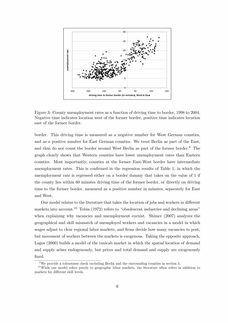
increasing the unemployment rates in Western border counties. Figure 3 shows the county

unemployment rates as a function of the driving time to the closest point on the former

6 In contrast to the summary statistics shown in Table 18, East and West refer here to the residence before

reunification.7Burda and Schmidt (1997) conclude that returns to education in the East were very similar to the

returns in the West, even in the early 1990s.8 Importantly, the model abstracts from migration. This assumption is discussed in detail in Section 3,

and relaxed in Section 6.2.

5

0

5

10

15

20

25

30

-350 -250 -150 -50 50 150 250

driving time to former border (in minutes), West to East

un

emp

loym

ent

rate

Figure 3: County unemployment rates as a function of driving time to border, 1998 to 2004.

Negative time indicates location west of the former border, positive time indicates location

east of the former border.

border. This driving time is measured as a negative number for West German counties,

and as a positive number for East German counties. We treat Berlin as part of the East,

and thus do not count the border around West Berlin as part of the former border.9 The

graph clearly shows that Western counties have lower unemployment rates than Eastern

counties. Most importantly, counties at the former East-West border have intermediate

unemployment rates. This is confirmed in the regression results of Table 1, in which the

unemployment rate is regressed either on a border dummy that takes on the value of 1 if

the county lies within 60 minutes driving time of the former border, or directly on driving

time to the former border, measured as a positive number in minutes, separately for East

and West.

Our model relates to the literature that takes the location of jobs and workers in different

markets into account.10 Tobin (1972) refers to “obsolescent industries and declining areas”

when explaining why vacancies and unemployment coexist. Shimer (2007) analyzes the

geographical and skill mismatch of unemployed workers and vacancies in a model in which

wages adjust to clear regional labor markets, and firms decide how many vacancies to post,

but movement of workers between the markets is exogenous. Taking the opposite approach,

Lagos (2000) builds a model of the taxicab market in which the spatial location of demand

and supply arises endogenously, but prices and total demand and supply are exogenously

fixed.

9We provide a robustness check excluding Berlin and the surrounding counties in section 5.10While our model refers purely to geographic labor markets, the literature often refers in addition to

markets for different skill levels.

6

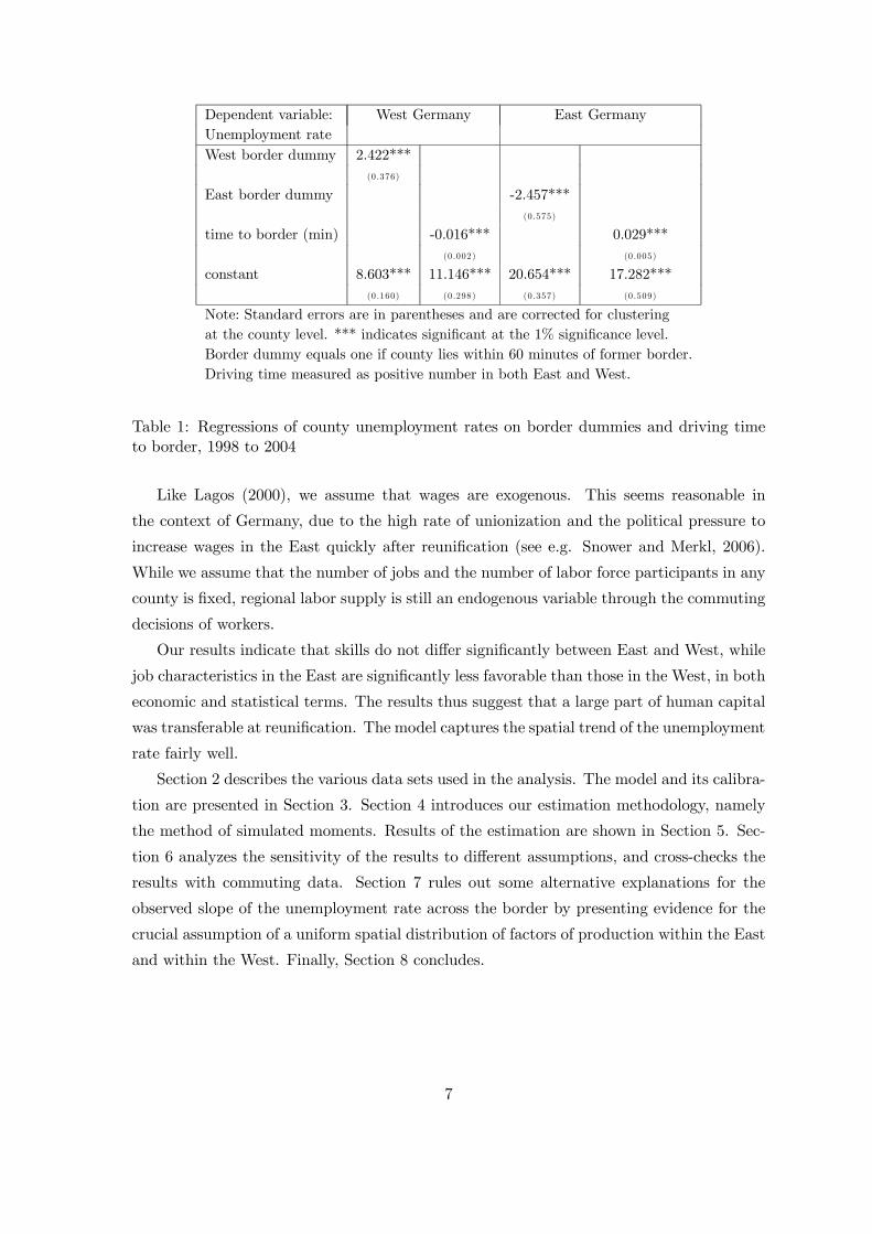
Dependent variable: West Germany East Germany

Unemployment rate

West border dummy 2.422***

(0.376)

East border dummy -2.457***

(0.575)

time to border (min) -0.016*** 0.029***

(0.002) (0.005)

constant 8.603*** 11.146*** 20.654*** 17.282***

(0.160) (0.298) (0.357) (0.509)

Note: Standard errors are in parentheses and are corrected for clustering

at the county level. *** indicates significant at the 1% significance level.

Border dummy equals one if county lies within 60 minutes of former border.

Driving time measured as positive number in both East and West.

Table 1: Regressions of county unemployment rates on border dummies and driving time

to border, 1998 to 2004

Like Lagos (2000), we assume that wages are exogenous. This seems reasonable in

the context of Germany, due to the high rate of unionization and the political pressure to

increase wages in the East quickly after reunification (see e.g. Snower and Merkl, 2006).

While we assume that the number of jobs and the number of labor force participants in any

county is fixed, regional labor supply is still an endogenous variable through the commuting

decisions of workers.

Our results indicate that skills do not differ significantly between East and West, while

job characteristics in the East are significantly less favorable than those in the West, in both

economic and statistical terms. The results thus suggest that a large part of human capital

was transferable at reunification. The model captures the spatial trend of the unemployment

rate fairly well.

Section 2 describes the various data sets used in the analysis. The model and its calibra-

tion are presented in Section 3. Section 4 introduces our estimation methodology, namely

the method of simulated moments. Results of the estimation are shown in Section 5. Sec-

tion 6 analyzes the sensitivity of the results to different assumptions, and cross-checks the

results with commuting data. Section 7 rules out some alternative explanations for the

observed slope of the unemployment rate across the border by presenting evidence for the

crucial assumption of a uniform spatial distribution of factors of production within the East

and within the West. Finally, Section 8 concludes.

7

2 Data

The main data for this project are monthly county level unemployment rates from 1998

to 2004, obtained from the German Institute for Employment Research (IAB). From these

data, we build the average county level unemployment rate from 1998 to 2004.11 Moreover,

in the calibration we use data from the IAB on the number of employed people per county

of residence, the number of employed people per county of work, the number of unemployed

per county of residence, and the number of vacancies posted at the employment agency of

the respective county.12

We also compare the predicted commuting streams from our model to actual cross-

county commuting data from 1999 to 2004. The commuting data cover only employees

who are subject to mandatory social insurance contributions (sozialversicherungspflichtig

Beschäftigte), which make up around 71 percent of all employees. For this reason, we match

the spatial distribution of unemployment rates rather than commuting flows directly.

For further evidence, we also use micro data from the German Socio-Economic Panel

(GSOEP) rounds 1998 to 2004. The German Socio-Economic Panel is an annual household

panel which allows the researcher to follow East and West Germans over time. We identify

a person as someone who lived in East Germany before 1990 if the person either belongs

to the “East Germany” sample that was added to GSOEP in the spring of 1990, or if the

person reports having a GDR-education.13 Appendix A presents some summary statistics

from work force characteristics in East and West based on the GSOEP data, and provides

evidence that differences in observable characteristics are very small. The estimations in

Section 7.1 aggregate data from GSOEP at the county level. There are four counties for

which we do not have any observations in GSOEP. Conditional on having a positive number

of observations, the mean number of observations per county over all seven years is 293,

and the median 231, with a minimum of 6 and a maximum of 2451.14

Last, we analyze aggregate data at the county level on investment subsidies, investment,

labor force participation rates, and plant openings. The first three data sets come from the

11A time-series analysis of these data shows no major time trends, but significant seasonality. The season-

ality pattern is similar for all counties, such that the average is a meaningful summary. Results are available

from the authors upon request.12These data are available for 2001.13The refreshment samples added in 1998 and 2000 do not directly identify the residence of the respondent

before reunification, but allows the researcher to deduce this residence from information about education.14To work with county identifiers, we use remote access to GSOEP via soepremote. When we use the data

without county identifiers, we work with the 95% random sample of GSOEP that is available for researchers

outside of Germany. The only sample restriction that we impose in Section 7.1 is that respondents have to

be at least 20 years old. The four counties with no observations are Stadtkreis Zweibrücken, Weiden in der

Oberpfalz, Memmingen, and Köthen. GSOEP treats Eisenach as part of the Wartburgkreis. Last, GSOEP

allows us to distinguish between East and West Berlin. However, in line with our main analysis, we treat

Berlin as part of the East. We repeat all regressions excluding Berlin, and the results are not sensitive to

the treatment of Berlin.

8

Bundesamt für Bauwesen und Raumordnung (various issues), and the latter data are based

on microdata from the IAB (Beschäftigtenstatistik). The data on investment subsidies

cover the period 1999 to 2003, the data on investment the period 1994 to 2002 in five time

intervals, the data on labor force participation rates are annual data from 1998 to 2004,

and the data on plant openings are annual data from 1996 to 2004.15

3 The Model

The model predicts the commuting behavior across counties and the resulting regional

unemployment rates based on the worker and job characteristic differences between East and

West Germany. It is a standard static frictionless two-sided matching model that matches

workers to jobs (see e.g. Roth and Sotomayor, 1990, for an exposition of a similar model).

The non-standard spatial component of the model arises through the spatial allocation of

jobs and workers, and through the parameterization of the cost of commuting.

3.1 Assumptions

Three strong assumptions of the model are the absence of migration, the fixed number of

jobs per county, and exogenous wage setting. We want to discuss these modeling choices in

some detail.

The model abstracts from migration, implicitly assuming that migration costs are pro-

hibitively high. Massive migration from the East to the West took place in the early 1990s.

Yet, since then migration flows have been relatively small. It is well established that unob-

served migration costs seem to be high in Germany, given that in general we do not observe

significant migration flows in response to economic conditions (e.g. Schündeln, 2005, and

Decressin, 1994). Hunt (2006) documents that East-West migrants are on average better

educated than stayers. One should keep in mind that the assumption of no self-selected

migration by skills biases us towards finding lower worker characteristics in the East than

in the West. Section 6.2 shows results from a sensitivity analysis that allows for random

migration prior to 1998.

We do not model job creation endogenously, but calibrate the number of jobs in each

county. Since we want to analyze whether unfavorable job characteristics or low human

capital in the East cause the low labor productivity, we remain agnostic about location

decisions of firms, and simply take them as given. The job characteristics in our model

could capture among others capital, government subsidies, and spill-over effects between

15The data on plant openings were aggregated by Michael Fritsch and are available at the webpage

http://www.wiwi.uni-jena.de/uiw/. In these data sets, we treat Hannover continually as one county. In the

data on investment and plant openings, which go back before 1998, we also treat Wartburgkreis/Eisenach

as one county, since it was only split in 1998.

9

firms, and modeling job creation further would require us to take up a stance on which of

these factors is especially important.

Wages in the model are exogenous and homogeneous within East and West, but poten-

tially differ between East and West. The assumption of an exogenous wage seems appro-

priate given the high rate of collective bargaining coverage in Germany. This is especially

true for East Germany, where the trade unions played a large role in wage determination

after reunification, partly due to the political fear of a large East-West migration (Snower

and Merkl, 2006).16 Kohaus and Schnabel (2003) report that 85 percent of employees in

the West and 80 percent of employees in the East were covered directly or indirectly by

collective bargaining agreements in 2000.17

3.2 Two-sided matching model

Labor productivity depends on workers’ skills and counties’ job characteristics , where

subscript indexes an individual, and subscript a county. Skill and job characteristic

distributions are the same for all counties in the East and all counties in the West, but

they potentially differ between East and West. Specifically, we assume that individual skill

levels are independently and normally distributed with mean in East, in West,

and the same variance 2 . We assume that the distribution of skills is identical in East

and West, since there are no significant differences in the standard deviations of years of

schooling between East and West, whether defined by current residence as in Table 18,

or by residence before reunification.18 Counties’ job characteristics are constant, and

equal to in the former East and in the former West. Evidence for the assumptions of

identical mean skills and job characteristics within the East and within the West is provided

in Section 7. We indicate as the wage paid in the county where job is allocated, and

as the wage paid in the home county of worker .

The net pay-off for a filled job is equal to the product generated by labor minus the

wage. The product generated by person in a job in county is a function of worker and

job characteristics. We assume the following functional form:

= ( ) = ∗ .

The net pay-off of a job in county j filled by worker i then amounts to

= ∗ −

16Snower and Merkl (2006) also show that, while the role of unions later declined, their legacy still persists.17According ot he OECD (1994), 90 percent of employees were covered by collective bargaining agreements

in West Germany in 1990.18While we argue that years of formal education are not a perfect measure of human capital, they are the

best available one. Section 6.1 shows results from a sensitivity analysis in which we assume a lower variance

in the East than in the West.

10

while an unfilled job generates a net pay-off of zero, = 0. Firms in county will not be

willing to employ individual if .

Commuting is possible but costly in the model. The cost of commuting of person from

home county to county is a function of the individual distaste of commuting and

the pairwise distance between counties and , . We assume ∼ [1 2]. The specific

functional form of the cost of commuting function = ( ) is given in Section 3.3.

The utility for worker being matched with job is equal to

= − ( )

while the utility of unemployment amounts to

= .

where is the unemployment replacement ratio that applies to the wage in the home

county.19 Therefore, an individual is willing to commute if

− .

Firms maximize their net pay-off and therefore prefer a higher skilled over a lower skilled

worker. Workers maximize their utility and therefore prefer a job in a nearby county to one

further away if both jobs pay the same wage. The solution algorithm to solve the model

numerically is described in Appendix B.

Note that in this model a qualified individual is not guaranteed to find work in her

home county. It might be that either there are not enough jobs available for all qualified

individuals living there, or that there are too many higher skilled workers in neighboring

counties that would like to commute into the home county. This can generate commuting

within the West and within the East. In addition, under the assumptions that and

= , the model will result in commuting from the East to the West across the former

border. This commuting occurs because some relatively high skilled individuals in the East

cannot find a job there since their product of labor is lower than the wage as a result of

the unfavorable job characteristics. Yet, these individuals are skilled enough to find a job

in the West, where the job characteristics are better. As a consequence, we also see more

commuting in the westward direction within the East and within the West. The westward

commuting within the West occurs because more skilled eastern workers fill western jobs,

and less skilled western job seekers have to find a job further into the West. The westward

commuting within the East occurs because the westward commuting of eastern workers

close to the border opens vacancies there for eastern workers living further into the East.

19The implicit assumption is that the unemployed person was previously employed in the home county.

11

Under the assumption of equal wages in East and West, the model predicts that, within

every county, the least skilled individuals are unemployed, and the most skilled individuals

work at home. Thus, relative to stayers, commuters are less skilled.20 Evidence for the

validity of these predictions can be found in the analysis of microdata on East German mi-

grants and commuters by Hunt (2006). Hunt (2006) finds that East German commuters are

not higher educated than stayers. Moreover, thirty percent of those beginning to commute

experienced a layoff in the previous year, which she interprets as pointing towards a compar-

atively low skill level of commuters. Last, Hunt (2006) finds that living in a county directly

bordering the West raises the probability of commuting to the West threefold. Thus, her

results are in line with the predictions of our model.

3.3 Parameterization and Calibration

In the baseline analysis, we assume that the wage is equal in East and West. The nominal

East-West ratio of wages shown in Figure 2 is smaller than one. However, since the tax

system is progressive, the after-tax East-West wage ratio is larger.21 Section 6.4 shows

results from a robustness check in which the wage in the East is assumed to be lower than

in the West. We set the wage equal to = 1, the infrastructure in the West equal to = 1,

and the variance of the skill distribution equal to 2 = 1. We discuss the normalizations

of and in Section 4.2, and estimate rather than calibrate the variance of the skill

distribution 2 in Section 6.1.

The unemployment replacement ratio is set to = 05, since the German unemployment

insurance system pays around 50 percent of the last income.22 The total number of available

jobs per county is equal to the number of people employed in each county, plus three times

the number of vacancies posted at the employment agency for the respective county, since

the IAB estimates that roughly a third of all vacancies are posted that way. The total

number of people in the labor force per county is set equal to the labor force in each county,

i.e. people living in each county who either work or are registered as unemployed. Figure

19 in Appendix C shows the difference between labor force and jobs in any county divided

by the labor force in that county. There is no spatial trend within the East or within the

West around the border due to the calibration of jobs and labor force participants, while

clearly jobs are more scarce in the East.

20Note that, under the alternative assumption , some East Germans who are skilled enough

to be offered a job in their home county still prefer a job in the West due to the higher wages, raising the

average skill level of East-West commuters somewhat (see Section 6.4).21Moreover, the price level in the East is still smaller than in the West, reducing the real wage difference.

Yet, commuters who primarily incur expenses in the county of origin might be more concerned about the

nominal than the real wage difference.22The replacement ratio is even higher for the first months (or years) of unemployment, where the length

of the period during which the higher replacement ratio is received depends on the length of the employment

history.

12

0

10

20

30

40

50

60

70

80

90

100

5 15 25 35 45 55 65 75 85 95

minutesp

erc

en

tag

e o

f p

op

ula

tio

n

Figure 4: Percentage of population willing to commute a certain number of minutes (one-

way)

The distance between two counties is measured as the driving time between the closest

points on a road to the centroids of the most populated Gemeinden of every county.23 All

interstates (Autobahnen) and larger roads (Bundesstrassen) are taken into account in this

calculation. We assume that the average driving speed on an interstate is 100 km/h, and

on the other roads 60 km/h.24 With this measure of distance, we calibrate the cost of

commuting to take the following form

( ) = 025

∙1 +

− min

max − min

¸where min corresponds to the minimum one-way driving time everyone is willing to com-

mute, and max to the maximum driving time beyond which nobody is willing to commute.

We calibrate min = 15 minutes and max = 100 minutes based on the reported will-

ingness to commute from two German surveys. One of these surveys (McKinsey et al.,

2005) asks whether a respondent would be willing to commute up to 2 hours per day (i.e.

two-way), and 31% of the respondents answer positively. Note that, interestingly, unem-

ployed people do not exhibit a higher willingness to commute in that survey than employed

people. In the other survey, conducted by the internet portal meinestadt.de in 2005, the

mean one-way distance individuals are willing to commute corresponds to 41 km. 75% of

respondents are willing to commute up to 20 km, 50% up to 30 km, 25% up to 50 km, and

10% up to 70 km.25 Figure 4 shows the percentage of the population willing to commute a

certain amount of time under our calibration, and it matches the numbers from the surveys

very well.

23There are between 6 and 235 Gemeinden in a county (Kreis).24Note that the average speed is smaller than the legal speed limit.25This survey question was answered by 10,006 respondents. The survey by McKinsey et al. has a sample

size of 510,000 individuals.

13

4 Identification and Estimation

We estimate the model using the method of simulated moments. The variables of interest

are , , and , with given. We define the two cut-off skill levels e and e as

the skill levels that satisfy e ≡ and e ≡

. Anyone with skills below these cut-

off skill levels is not qualified to work in East or West, respectively. The parameters to be

estimated are the mean skill in the West , the difference in the cut-off skill levels e− e ,and the difference in mean skills − . Thus, the parameter vector comprises =n e − e −

o.26 This parameter vector implicitly defines the three underlying

variables of interest. We choose these specific parameters since they are largely immune to

the normalizations, as discussed in Section 4.2.

4.1 Identification

The model is identified through the regional behavior of the unemployment rate, and espe-

cially the behavior of the unemployment rate in the border area.

Given , , and 2 , the average unemployment rate in the West pins down . In

fact, if there were no East-West commuting, and if we would treat the West as one labor

market area with unemployment rate , the mean West skills could be derived

analytically. Let () be the probability distribution function associated with mean skills

in the West and variance 2 , then would be implicitly determined by the condition

³ e´ = R

−∞ () = .

Any increase in the differences in skills or differences in job characteristics between East

and West leads to an increase in the difference of the mean unemployment rates, and thus

to an increase in the average East unemployment rate.27 However, an increase in the skill

difference − leads to a sharper increase in unemployment rates across the border

since less commuting takes place, while an increase in the difference of the cut-off skill

levels e − e (which implies an increase in the difference of job characteristics) leads

to a flatter increase through more commuting. Thus, while an increase in any of these

differences leads to a higher average unemployment rate in the East, the effect on the slope

of the unemployment rate across the border goes in different directions, and therefore both

differences are identified.28

The variation in the unemployment rate in the model comes from the spatial position

26Defined this way, these differences are positive if in fact and .27For expositional simplicity, we assume here that the East does not look more favorable in either skills

or job characteristics, but the logic holds true if this is not the case.28 I.e. the average unemployment rate in the East could be matched by a continuum of combinations of

− and − , with both differences being negatively correlated, but each of these combinationswould predict a different slope of the unemployment rate across the former border.

14

0

5

10

15

20

25

West>100

West60-100

West40-60

West20-40

West 0-20

East 0-20

East20-40

East40-60

East60-100

East>100

un

em

plo

ym

en

t ra

te

Figure 5: Average unemployment rates of different regions, constructed according to driving

time to former border (in minutes).

of the counties, and the calibrated number of jobs and number of people in the labor force.

Within the East and within the West, the model allows for no further variation, e.g. in

the form of rural and urban areas, or to capture the general North-South trend in the

unemployment rate.29 It therefore underpredicts the variance of the unemployment rate,

especially in the West. We choose to abstract from modelling these additional features, and

instead assume that they are orthogonal to the model. The moments to be matched are

then regional unemployment rates, with the underlying assumption that these additional

features average out within every region.

Given the identification, we choose to approximate the slope of the unemployment rate

along the border through a step function, and to match the average unemployment rates

of ten regions, putting special emphasis on regions close to the border. For East and West

separately, we construct the average unemployment rate of all counties within 20 minutes

driving time to the border, those with a driving time to the border between 20 and 40

minutes, between 40 and 60 minutes, between 60 and 100 minutes, and all counties with

a driving time to the border of more than 100 minutes.30 Figure 5 shows the average

unemployment rates of these regions; they are monotonically increasing as one moves from

West to East.

29Note that the model captures part of the decreasing North-South trend in unemployment rates within

the West, since more northern counties in the West are affected by East commuters than southern counties.30Since there is not much variation in the average unemployment rates further than 100 minutes away

from the border, and since the cost function is specified such that noone is willing to commute more than

100 minutes, we choose not to break down the region beyond 100 minutes from the border into further

subregions.

15

4.2 Normalizations

Why do we choose to estimate e − e and − , rather than e.g. the ratios

and

, or directly and ? Note that they all are equivalent transformations, and thus in

principle the choice does not matter. The reason why we pick the differences e − e and

− is that they are immune to the chosen normalizations, namely to the normalizationson and .

To see why this is the case, assume that we have estimated the parameters ∗ ³e − e´∗

and ( − )∗ given the fixed parameters ∗ and ∗. Now consider a change in the pa-

rameterization of either the wage to ∗∗ and/or of the West job characteristics to ∗∗ ,

resulting in a change of the West cut-off skill level from e∗ to e∗∗ . In order to obtainexactly the same predicted unemployment rates, we have to shift both the East and West

skill distributions and the cut-off skill level in the East by exactly the same amount, i.e. bye∗∗ − e∗ . As a consequence, the estimates of e − e and − remain unchanged,

and only the estimate of changes to ∗∗ = ∗ + (e∗∗ − e∗ ). Thus, the estimates ofinterest, as well as their standard errors, are unaffected by the assumptions on and .

4.3 Method of Simulated Moments

Let () be the average unemployment rate of region , and let be the unemploy-

ment rate of county in region . Moreover, let =n0

³e − e´

0 ( − )0

obe

the true parameter vector. For every region , the following moment condition holds

¡ (0)

¢=

¡

− ()¢= 0

We use the method of simulated moments (Pakes and Pollard, 1989) to find the parameter

estimates that minimize

min

c ()0c ()

where c () is a column vector of size ten, and each element of c equals the empirical

counterpart c = 1

P

³

−d

()´of the above stated moment condition. is

the number of counties in region , and d

() is the average simulated unemployment

rate in region , given the parameter vector .

We apply a two-step procedure. In the first step, which provides consistent estimates

of the parameter vector, the weight matrix is equal to the identity matrix, = . The

variance of the moment estimates is defined as Ω = ¡ () ()0

¢. In the second

step, we use the inverse of an estimate bΩ of this matrix as the weight matrix, = bΩ−1 ,

16

reoptimize, and get efficient estimates of the parameter vector.31 Define derivatives of the

moment condition with respect to the parameter vector as = (). The variance

of the parameter estimates in the second step is then equal to Ω =¡1 + 1

¢ ³0Ω

−1

´,

and an estimate bΩ of Ω is used to calculate standard errors for our estimates of . equals the number of simulations. In the estimate bΩ, Ω−1 is replaced with the estimatebΩ−1 , and the derivatives are replaced with consistent numerical analogues. Under the

regularity conditions stated in Pakes and Pollard (1989), the MSM estimator is consistent

and asymptotically normally distributed.

We solve the model using pattern search as a minimization algorithm. While the crite-

rion function of this problem is convex, it is not continuous due to the discretization into

counties, necessitating a minimization algorithm that does not use the gradient to search

for an optimal point. Note that the criterion function has no local minima, yet exhibits a

plateau. Due to the calibrated number of jobs and people in the labor force, the predicted

unemployment rates cannot fall below certain levels. Thus, at some point an increase in the

worker and job characteristics in East and West leads to no further decline in the predicted

unemployment rates. Based on grid searches, we make sure that there is indeed a minimum,

and that our minimization algorithm does not stop on a plateau but leads to the global

minimum. We divide both the number of jobs and the number of people in the labor force

by 100, and use 50 simulations.

5 Results

Table 2 presents the results. Strikingly, the estimated West-East skill difference is negative.

Thus, East skills are even higher than West skills. Yet, as the 95% confidence intervals show,

this difference is not statistically significant. Thus, either human capital accumulated in

the East did not depreciate at reunification, or eight years were enough to accumulate

new specific human capital, potentially aided by public policy programs with regard to

retraining. Early retirement policies after reunification probably make the picture more

favorable for skill differences than it would otherwise have been, since older workers should

have accumulated more specific human capital, and were more likely to exit the labor market

after reunification. On the other hand, selected migration might have lowered the mean

skills in the East; Hunt (2006) shows evidence that emigrants are on average more skilled

than stayers.

Friedberg (2000) analyzes the return to foreign education of immigrants into Israel and

finds that, while it is initially lower than the return to native education, acquiring further

31 Ω is a diagonal matrix, where the t-th element equals Ω = 1

−

()2.

17

95% confidence

coeff. interval

2.4779

(0.0995)e−e 0.7065

(0.1816)

− -0.2315

(0.0988)

2.4779 [2.2829 2.6729]

implied 2.7094 [2.5157 2.9031]

implied 0.5860 [0.4849 0.7404]

Note: Standard errors are in parentheses

Table 2: Results from baseline calibration

human capital following immigration can raise these returns even above the returns of

natives. It might be the case that, parallel to her findings, the general good schooling in

the East combined with some years of labor market experience in the West increases the

skill levels of East Germans above the average levels of West Germans.

In contrast to skills, the East job characteristics amount to = 05860, and are thus

lower than the West job characteristics of = 1. This difference is significant at the 1%

significance level. Hence, our results indicate that unfavorable job characteristics in the

East are the driving force of the low labor productivity there. We want to stress again that

“job characteristics” in our model capture anything that has a positive influence on labor

productivity, but cannot be directly influenced by the worker (e.g., infrastructure, physical

capital, network effects between firms). Clearly, several of these factors could be at play,

and could together explain the difference. The large financial subsidy programs encouraging

firms to invest in the East somehow seem to have failed to produce the same quality of jobs

in the East as in the West. We provide further discussion of the results in the conclusion.

Figure 6 shows the resulting simulated unemployment rates for the counties based on

100 simulations, plotted against the driving time to the border, as well as the actual unem-

ployment rates from the data. Our model matches the slope fairly well, but fails to produce

enough variation in the Western counties more than 100 minutes away from the border.32

This is not surprising, given that in the model the only heterogeneity of counties within the

East or within the West arises through the calibrated number of jobs and number of people

in the labor force.

32Specifically, note that, as explained in Section 4.1, the estimate of effectively sets a lower bound

for the predicted unemployment rate in the Western counties further away from the border. The residuals

show some remaining spatial correlation which levels off at 200 kilometers, but they do not have a significant

East-West trend.

18

0

5

10

15

20

25

30

35

-350 -300 -250 -200 -150 -100 -50 0 50 100 150 200 250

driving time to former border (in minutes), West to East

Actual UR

Simulated UR

Figure 6: Actual and simulated unemployment rates as a function of driving time to former

East-West border

In this analysis, we treat Berlin as part of the East. As a robustness check, we repeat

the analysis excluding Berlin and the nine counties directly bordering Berlin. The estimates

are very similar, and we are therefore confident that our treatment of Berlin is not crucial

for the results. We also estimate the model using a finer definition of regions around the

border, namely 15 minutes intervals of driving time to the former border, up to 60 minutes

away from the border. Again, the results are qualitatively and quantitatively very similar.33

Older workers are typically assumed to have accumulated more specific skills through ac-

cumulated experience in an industry or a firm. Therefore, skill depreciation at reunification

might have affected older workers more than younger ones. To gain some insights into this

hypothesis, we construct unemployment rates for 50 to 64 years old workers, and use these

unemployment rates as moments to be matched by the model.34 This exercise relies on the

crucial assumption that the allocation of workers and jobs is the same for the old as for

the entire population. Table 3 shows the results. For the older population, the East-West

skill difference is almost zero. Compared to the overall population, the skill advantage of

East Germans thus disappears, but does not turn into the opposite. This is an indication

for more skill depreciation for older workers.35 Note that the mean estimated skills in the

West are lower here than in the baseline results, since unemployment rates in the West are

33Results are available from the authors upon request.34We have age-specific data on the number of unemployed and employees subject to mandatory insurance

contributions on the county level. To construct age-specific unemployment rates, we assume that the age

distribution of civil servants and part-time employees matches the one of mandatorily insured employees.35Self-selection into early retirement, as well as lower migration rates than for the younger population

might lead to an overestimation of the skill levels of the older workers as compared to the entire working

age population.

19

higher for the older population. The estimated job characteristics in the East are somewhat

more favorable than in the baseline results, but remain significantly less favorable than in

the West.

95% confidence

coeff. interval

2.2377

(0.0760)e−e 0.5775

(0.1498)

− -0.0335

(0.0191)

2.2377 [2.0887 2.3866]

implied 2.2712 [2.2338 2.3086]

implied 0.6339 [0.5344 0.7789]


Table 3: Results from model matched to unemployment rates of older workers

6 Robustness Checks

In this section, we carry out a variety of robustness checks. First, we estimate the variance

of the skill distribution in addition to the other three parameters, and additionally carry

out a sensitivity analysis in which we set the variance of the skill distribution to a lower

level in the East than the one in the West. Second, we present results based on a calibration

that allows for migration before 1998. Third, we analyze the sensitivity of the results with

regard to the assumed willingness to commute. Fourth, we discuss how the results change

if the wage in the East is assumed to be lower than that in the West. Last, we present

some evidence how the predicted commuting from the baseline results matches with actual

commuting behavior.

6.1 Variance of the Skill Distribution

In the baseline calibration, the variance of the skill distribution is set to 2 = 1. In this

section, we estimate the variance of the skill distribution in addition to the other three para-

meters, such that the parameter vector is now =n2 e − e −

o. Table 4

shows the results. The point estimate of the variance is 0.89, but it is not significantly differ-

ent from one. Moreover, the estimates of our variables of interest remain almost unchanged,

both in an economic and in a statistical sense.36

36We also ran robustness checks in which we calibrated the variance to be 2 = 08 or 2 = 12, respec-

tively. Again, the changes in the estimates are minor.

20

95% confidence

coeff. interval

2 0.8932

(0.0699)

2.3995

(0.1353)e−e 0.6578

(0.1497)

− -0.2092

(0.0698)

2 0.8932 [0.7563 1.0301]

2.3995 [2.1344 2.6647]

implied 2.6087 [2.4718 2.7456]

implied 0.6032 [0.5125 0.7329]


Table 4: Results adding variance of skill distribution as fourth parameter

95% confidence

coeff. interval

2.4778

(0.0875)e−e 0.6776

(0.0837)

− -0.0986

(0.0200)

2.4778 [2.3062 2.6494]

implied 2.5764 [2.5373 2.6155]

implied 0.5961 [0.5430 0.6607]


Table 5: Results with smaller variance of skill distribution in East than in West

21

One might also be worried that the variance of the skill distribution is smaller in the

East than in the West. While Table 18 shows that the variance of years of formal education

is slightly larger in the East than in the West, one might still expect a smaller variance

of worker characteristics. If specific human capital mattered a lot and depreciation at

reunification was substantial, this could have not only lowered the mean skill in the East

but also the variance. While our baseline results do not indicate that this was the case, we

nevertheless run a robustness check in which we keep the variance of the skill distribution

at one in the West, i.e. 2= 1, but lower it to 0.8 in the East, i.e. 2= 08. Table 5

shows the results. The results indicate a slightly smaller skill advantage in the East relative

to the baseline results. However, none of the results change significantly. Summarizing, we

conclude that the results are not very sensitive to assumptions about the variances of the

skill distributions.

6.2 Migration

So far, the analysis abstracts from migration and assumes that all individuals currently

residing in East Germany have skills drawn from the East distribution, and all individuals

currently residing in West Germany have skills drawn from the West distribution. However,

migration in the early 1990s between East and West was substantial, although it declined

by the mid 1990s. Since we hypothesize that skills in East and West could differ because of

the education and job experience accumulated before 1990, this migration could potentially

matter for our analysis. In this robustness check, we allow for migration before our sample

period.

95% confidence

coeff. interval

2.4632

(0.1094)e−e 0.6946

(0.1337)

− -0.2714

(0.2440)

2.4632 [2.2488 2.6776]

implied 2.7346 [2.2564 3.2129]

implied 0.5904 [0.5111 0.6981]


Table 6: Results allowing for migration before 1998

From the 1998 to 2004 rounds of the German Socio-Economic Panel, we obtain an

estimate of the percentage of the population that is originally from East Germany for every

22

county. Now, in the first step of our solution algorithm outlined in Appendix B, we draw

skills from the East and West distributions for the population of every county not simply

according to whether the county is located in the East or in the West, but according to the

estimated percentage of individuals originally from the East and originally from the West.37

Note that an underlying assumption of this exercise is that migrants are not self-selected.

Hunt (2006) provides evidence that migrants are on average better educated than stayers.

Thus, our results might still be biased in the direction of underestimating the average skill

level of individuals who lived in East Germany before reunification. Table 6 shows the

estimated parameters using this additional information. The estimates change only very

slightly, and certainly not significantly. This is expected if migrants settled rather uniformly

in the respective other part of the country. Section 7.1 provides a further analysis of this

issue.

6.3 Cost of Commuting

Since the identification of the model relies on commuting behavior, the assumed cost of

commuting is important. Although we calibrate this cost such that the willingness to

commute matches evidence from survey data, we analyze how results change if we assume a

lower cost of commuting. A lower cost of commuting clearly leads to more commuting; thus,

intuitively, in order to still match the slope of the unemployment rate across the border,

the estimates have to change in order to decrease commuting again, namely in the direction

of lower skills in the East than in the West, with more similar job characteristics in East

and West.

95% confidence

coeff. interval

2.3504

(0.0466)e−e 0.4646

(0.0352)

− 0.1380

(0.0100)

2.3504 [2.2590 2.4418]

implied 2.2124 [2.1927 2.2321]

implied 0.6828 [0.6520 0.7166]


Table 7: Results from different calibration of cost of commuting

37As an example, for the first county, Flensburg, which is located in the West, we estimate that 94.8

percent of individuals living there are originally from the West. We draw skills from the West distribution

for 94.8 percent of the calibrated labor force and skills from the East distribution for the other 5.2 percent.

23

Table 7 shows the results for an alternative calibration, in which the minimum and

maximum amounts of time anyone is willing to commute are doubled from min = 15minutes

and max = 100 minutes in the baseline calibration to min = 30 minutes and max = 200

minutes. This calibration implies that everyone is willing to commute 30 minutes each

way to work, and that more than two third of the population are willing to commute one

hour each way.38 When the willingness to commute is basically doubled from the baseline

calibration, the estimated mean skill in the East becomes smaller than the mean skill in

the West. While this difference is statistically significant, it is small in absolute terms.

Moreover, the job characteristics in the East remain significantly less favorable than in the

West, and the East-West difference in job characteristics is still much more pronounced

than the difference in skills.

6.4 East-West Differences in Wages

Pre-tax East wages are still lower than West wages in nominal terms.39 To allow for lower

wages in the East, we have to modify the model somewhat. First, we change the cost of

commuting to ensure that the willingness to commute is independent of the counties of

origin and destination.40 Second, if a job in the West pays a higher wage than a job in the

East, then some East Germans who could find a job in the East may prefer to commute

further into the West, since the net return to working there (i.e. the wage minus the cost

of commuting) may be larger than the net return to working in a closer East county. Thus,

individuals do not simply minimize the cost of commuting anymore, but rather maximize

the net return to working. This modification increases the willingness to commute from the

East to the West.41

Table 8 shows results when the wage in the East is set to = 085, while the wage in

the West is kept at = 1.42 The implied skill level in the East is now smaller than in the

38Remember that survey evidence suggests that only one third of the population are willing to commute

one hour each way.39There is no significant evidence for a spatial trend in the wage data on the county level. A regression of

wages from 1998 to 2003 on a border dummy (that takes on the value one if a county lies within 60 minutes

driving time of former border) shows that wages are 2.2 % lower in the West border area than in the rest of

the West, but with a p-value of only 0.23. In the East, there is no evidence at all for different wage levels in

the border area. Results are available upon request.40This is achieved by assuming that an individual is willing to commute whenever 05, correspond-

ing to the baseline calibration. Otherwise, we would have to take a stance on which wage, namely from

the county of origin or destination, determines the unemployment replacement benefit. Moreover, we do

not have any survey evidence on willingness to commute depending on whether the counties of origin and

destination lie in East or West.41 If the lower wage would be paid to any East German, regardless of the county where the job is located,

then the incentives for East Germans to commute would remain unchanged. As a consequence, none of the

three estimates from the baseline calibration would change.42The choice of = 085 is motivated by the fact that income tax reports on the state level show that

in 2001, the average tax rate of East Germans is around 5 percentage points higher than the average tax

rate of West Germans, such that the after-tax East-West wage difference is smaller than the pre-tax wage

24

95% confidence

coeff. interval

2.5325

(0.0781)e−e 0.1358

(0.0899)

− 0.3765

(0.1199)

2.5325 [2.3793 2.6856]

implied 2.1560 [1.9210 2.3909]

implied 0.7483 [0.6479 0.8857]


Table 8: Results from calibration with lower East wages

West, but not significantly so at the 5 percent significance level.43 The job characteristics

remain clearly significantly less favorable in the East than in the West.44 Thus, allowing

for a lower wage in the East reduces the estimated mean skill in the East to a level lower

than that in the West, but still identifies the job characteristics as the main driving force

of the lower labor productivity in the East.

6.5 Commuting in Model and Data

Commuting data is only available for 71 percent of all employed people, namely employees

who are subject to mandatory social insurance contributions. This is the main reason why

we match the model to unemployment rates instead of commuting, and has to be kept in

mind when comparing these data to commuting data generated by the model.45 For em-

ployees who are subject to mandatory social insurance contributions, we have information

on commuting between all 439 counties for the years 1999 to 2004 from the German Em-

ployment Agency. We take averages of the county-to-county commuting streams over these

six years to compare commuting patterns in the data to the ones generated by our model.

The model underestimates the total amount of cross-county commuting significantly.

In the model, 7.5 percent of all employed people commute, while in the data 35.0 percent

commute. There are two reasons why the model underestimates commuting. First, in the

difference.43The East-West ratio of mean skills according to the point estimates equals almost exactly the East-West

ratio of wages.44Note that − is now defined as − =

−

. Thus, an estimate close to zero does not

indicate equality of job characteristics in East and West, in contrast to the baseline calibration.45 It might be reasonable to assume that the omitted 30 percent commute less than the covered 70 percent.

Civil servants are in tenured positions and thus have a longer planning horizon when making their residence

decision. For part-time workers, commuting is especially costly given the fixed nature of commuting per

working day.

25

model commuting always occurs in only one direction, since there exists no random com-

muting that is not driven by economic incentives. Second, by assumption noone commutes

more than 100 minutes one way in the model. Focusing on net commuting in the data, the

percentage of commuters falls by more than a half to 16.2 percent, i.e. random commuting

accounts for more than half of total commuting.46 Of all commuters in the data, 89 percent

commute less than 100 minutes. Table 9 reports the percentage of all employees commuting

a certain amount of minutes one-way to work in the data, separately for gross and net com-

muting streams. These data are scaled by the number of employees in counties of origin for

which the set of other counties within the analyzed driving time is not empty.47 The per-

centage of commuters is declining drastically in the data within 100 minutes driving time,

which is consistent with the survey evidence that we use to calibrate the cost of commut-

ing. Between 100 and 300 minutes driving time, the percentage of commuters is relatively

constant at around 0.6 percent gross and 0.3 percent net. After 300 minutes, it falls further

towards zero. Thus, there is a non-negligible amount of probably weekly commuting in

the data that we do not model, since by assumption in the model noone commutes further

than 100 minutes. One should also keep in mind that there are tax incentives in favor of

reporting a second residence for commuting reasons, which might lead to an overprediction

of actual commuting in the data.

To further analyze whether the predicted East-West commuting by the model matches

up with the data apart from the level effect of lower commuting in the model, we show two

pieces of evidence. First, Figure 7 shows the percentage of East-West commuters relative

to all employees in the East counties as a function of the driving time to the former border

in data and model.48 This critical statistic is matched fairly well by our model. While

the model underpredicts East-West commuting, and by assumption sets it equal to zero

for counties further than 100 minutes away from the border, it nevertheless captures the

increase towards the border observed in the data. Figure 20 in Appendix D shows that

similarly the data also exhibit a slope towards the border in the West if one analyzes the

percentage of East in-commuters relative to the entire labor force working in the host county.

Part of this increase in East-West commuters towards the border is however solely

46Of course, this commuting is only random in the sense of the model, which assumes a homogeneous

labor market.47For short driving times, the scaling factor is simply the total number of employees in Germany. The

scaling procedure only becomes important when we analyze longer driving times, since e.g. not all of the

counties have another county that is eight hours driving time away. Through our procedure we take this

into account, such that the percentage of commuters does not simply decline with driving time due to the

decline in the number of possible commuters.48Note that due to systematic East-West commuting the difference between gross and net commuters is

much smaller when focusing on East-West commuting than in the data in general. Overall, 6.7% of all

East employees commute into the West when analyzing gross commuting, and 5.5% when analyzing net

commuting.

26

commuting time (in minutes) percentage commuting (gross) percentage commuting (net)

0-20 18.11 8.57

20-40 12.88 5.84

40-60 5.05 2.24

60-80 2.15 0.94

80-100 1.09 0.51

100-120 0.58 0.28

120-150 0.69 0.33

150-180 0.46 0.23

180-240 0.69 0.35

240-300 0.58 0.32

300-360 0.47 0.26

360-420 0.30 0.15

420-480 0.11 0.05

480-540 0.06 0.03

540-600 0.02 0.01

over 600 0.01 0.005

Table 9: Percentage of commuters relative to all employed people in counties of origin by

commuting time, 1999 to 2004.

0.1

.2.3

0 50 100 150 200time to border

gross data net datasimulation

Figure 7: East-West commuters as percentage of employed people in origin county in East

in data and simulations.

27

a consequence of the fact that we are focusing on cross-border commuters here. Some

increase in cross-border commuting would be expected towards any fictional border. To see

whether there is something special about the former East-West border, we run a regression

of the percentage of all commuters (i.e. not focusing solely on commuters into the West)

relative to employees in the East on driving time to the former border, either linearly or

on time group dummies. This variable should capture whether commuting systematically

increases towards the border. We control for the size of the county, since smaller counties

systematically report higher commuting rates due to the discretization of commuting into

counties. Results are reported in Table 10. While clearly the level of predicted commuting

is too small compared to the level of actual commuting, the increase in commuting towards

the border is quite similar in data and simulations.

Dependent variable: gross data net data simulations

% commuters

time to border¡∗103¢ -0.404** -0.476*** -0.559***

(0.186) (0.143) (0.125)

0-20 minutes 0.059* 0.083*** 0.089***

(0.036) (0.028) (0.025)

20-40 minutes 0.045 0.052** 0.055***

(0.029) (0.022) (0.020)

40-60 minutes 0.036 0.032 0.042**

(0.029) (0.022) (0.020)

60-80 minutes 0.064** 0.053** 0.055***

(0.028) (0.022) (0.019)

80-100 minutes 0.074** 0.026 0.036*

(0.029) (0.022) (0.020)

square km¡∗103¢ 0.028** 0.026** 0.055*** 0.055*** 0.030*** 0.030***

(0.013) (0.013) (0.010) (0.010) (0.009) (0.009)

constant 0.298*** 0.371*** 0.102*** 0.173*** 0.052*** 0.134***

(0.022) (0.019) (0.017) (0.015) (0.015) (0.013)

Note: Standard errors are in parentheses. *** indicates signficance at the 1%,

** at the 5%, and * at 10% significance level. Time dummies equal one if driving time

to former border amounts to given minutes.

Table 10: Regressions of percentage commuters on driving time to border dummies and

driving time to border, actual and simulated data.

7 Alternative Hypotheses

The model explains the slope of the unemployment rate across the border through com-

muting behavior. However, one could potentially imagine other reasons for the gradual

increase in the unemployment rates across the former border. The most important alter-

native hypotheses have to do with the spatial allocation of factors of production. Note

28

especially that the model assumes that every county within the East has the same mean

skills and job characteristics, and the same holds true within the West.49 It could however

be possible that either human capital or physical capital are allocated in Germany such

that the level and quality is gradually decreasing as one moves from West to East. In that

case, the unemployment rate would gradually increase even if all factors of production were

only employed in the home county, and thus there would be no commuting. The following

two subsections provide evidence on the spatial distribution of human and physical capital

within the East and within the West. The third subsection addresses the issue of market

access.

7.1 Spatial Distribution of Skills

The model abstracts from migration and assumes the same distribution of skills for every

county within the East and within the West. It could however be possible that skill levels

are not only higher in West Germany than in the East, but gradually decreasing as one

crosses the border. Under the assumption that Eastern skills depreciated somewhat at

reunification, for the Eastern side of the border this would mean that either more “West

Germans”, i.e. individuals who acquired human capital in the West, are settled there than

in the rest of the East, or on average higher skilled people are settled there than in the rest

of the East. For the Western side of the border, this would mean that either more “East

Germans”, i.e. individuals who acquired human capital in the GDR, or lower skilled people,

settle there than in the rest of the West.

From GSOEP, we get information for every county about the estimated percentage of

the population that is originally from West Germany, as described in Section 6.2. Moreover,

we derive the highest educational degree of the respondent, analyzing the categories college,

vocational training, secondary schooling, and no school degree, and then calculate the per-

centage of respondents within a county belonging to each educational category. We regress

both the East/West composition and the educational attainment on border dummies, as

well as on the driving time to the former border.50 We separately create a West border

dummy for counties within 60 minutes driving time to the West of the former border, and

an East border dummy for counties within 60 minutes driving time to the East.

As Table 11 shows, a relatively lower percentage of the population in the Western border

counties is from the former West, and the percentage of the population from the former

West is generally increasing as one moves away from the border in the West. However,

in East Germany the composition of the population does not seem to be influenced by

49We relaxed this assumption already in the robustness check in Subsection 6.2.50The individual data are aggregated at the county level separately for every year. The standard errors

in the regressions are corrected for clustering at the county level.

29


% of West Germans

West border dummy -0.045***

(0.017)

East border dummy -0.018

(0.017)

time to border¡∗103¢ 0.200*** 0.086

(0.077) (0.156)

constant 0.953*** 0.918*** 0.099*** 0.085***

(0.005) (0.013) (0.014) (0.011)

Note: Standard errors are in parentheses and are corrected for

clustering at the county level. *** indicates significant at the 1%

significance level. Border dummy equals one if county lies within

60 minutes driving time of former border. Driving time to border

measured as positive number in both East and West.

Table 11: Regressions of percentage of West Germans in population on border dummies

and driving time to border, 1998 to 2004


% college degree

West border dummy -0.012

(0.016)


(0.017)

time to border¡∗103¢ 0.050 0.138

(0.075) (0.153)

constant 0.147*** 0.139*** 0.226*** 0.209***

(0.006) (0.012) (0.011) (0.015)






Table 12: Regressions of percentage of population with college degree on border dummies

and driving time to border, 1998 to 2004

30

the distance to the border. Moreover, Table 12 shows that the skill composition is not

significantly different in the border areas from the rest in neither East nor West. We test

this by analyzing the percentage of the population with college degree, but similar results

arise if we use total years of formal education as the dependent variable. Summarizing,

any evidence that the skill composition differs between counties comes from West Germany

alone. However, even in the West the quantities are relatively small: while 95.3% of the

population living in West German counties away from the border is from the former West,

this percentage declines to 90.8% in the Western border counties.51


labor force participation rate

West border dummy 1.305***

(0.413)

East border dummy 0.601

(0.387)

time to border¡∗103¢ -0.010*** -0.006

(0.003) (0.004)

constant 65.2*** 66.8*** 68.3*** 39.0***

(0.2) (0 .4) (0 .3) (0 .4)






Table 13: Regressions of labor force participation rates on border dummies and driving

time to border, 1998 to 2004

We also analyze whether labor force participation rates differ systematically across space,

which could indicate that all that is differing across counties is how people assign themselves

as being either unemployed or out of the labor force. Especially if labor force participation

rates were increasing systematically across the border from West to East, this could explain

why unemployment rates also increase.52 Indeed, the mean labor force participation rate

across counties amounts to 65.4 percent in the West, and 68.5 percent in the East. Table 13

shows the results of a regression of the county level labor force participation rates on driving

51 If we weigh counties by the number of individual observations used to construct the county aggregates,

such that counties for which aggregates are estimated with higher precision obtain a larger weight, results

are only slightly different. Most importantly, they indicate that the percentage of the population originally

from the West is slightly lower in the East border region than in the rest of the East, as is the percentage of

individuals with college degree. Both results are significant at the 10% significance level. Thus, if anything,

individuals living close to the border in the East seem to be less skilled than individuals living in the rest of

the East. Results are available upon request.52This hypothesis is likely to be true to some extent since labor force participation rates in the GDR were

substantially higher than in the former West Germany, especially among women. Bonin and Euwals (2002)

argue that part of the East-West unemployment rate difference can be explained through the differential

labor force participation of women.

31

time to the border. In West Germany, the labor force participation rate is significantly

higher in the border counties. The counties within 60 minutes driving time to the former

border in the West have a labor force participation rate that is 1.3 percentage points higher

than in counties further away from the border, but an unemployment rate that is 2.4

percentage points higher (see Table 1). However, labor force participation rates in the East

do not exhibit a significant spatial trend.

7.2 Spatial Distribution of Physical Capital

The model also assumes that job characteristics are homogeneous within the East and the

West. One might be worried that public infrastructure investment or public subsidies to

firms in the East were targeted towards the border area, thus generating more favorable job

characteristics close to the former border, as opposed to further East. Note, however, that

public transfers into the East are either generated by the German regional transfer system,

which seeks to equalize living conditions across Germany, or specific to East Germany.

The former implies that regions with the worst economic conditions receive the largest

transfers. Transfers within the latter category do not discriminate geographically within the

East. The most important specific investment subsidy program for the East (Investitions-

zulagegesetz) specifies by law that subsidies are to be given to all applicable investments,

as long as the investment takes place in the East. In fact, one of the major criticism of the

vast West-East transfer programs is that they do not focus on certain regions, but rather

work indiscriminately. Some subsidy programs apply only to economically underdeveloped

areas.53 These areas include all Western counties at the former border,54 some selected

areas in the West further away from the border, and the entire East. I.e. these programs do

not discriminate against West border regions, as compared to the rest of the West; neither

do they favor East border regions, as compared to the East. They rather do the opposite

in the West, and apply to the entire East. While it is hard to get data at the county level,

the Deutsche Bank (2004) for example reports that total investment subsidies for the East

from 1990 to 2004 amounted to 18,400 Euro per person. This amount only varied between

the five Eastern states from a minimum of 16,770 Euro in Brandenburg to a maximum of

19,890 Euro in Sachsen-Anhalt.

From the Bundesamt für Bauwesen und Raumordnung (2005), we have data on subsidies

at the county level from a fairly extensive list of programs from 1999 to 2003.55 These

53These are the programs under the heading Gemeinschaftsaufgabe Verbesserung der regionalen

Wirtschaftsstruktur.54The former border areas (Zonenrandgebiete) received special federal subsidies before reunification, and

continue to do so to a lesser extent today.55The data report amounts for the entire time period, not annual amounts. The programs are: ERP

Eigenkapitalhilfeprogramm, ERP Existenzgründungsprogramm, KfW Mittelstandsprogramm, ERP Regional-

programm, ERP Innovationsprogramm, ERP Umweltprogramm, GRW gewerbliche Wirtschaft, GRW Frem-

32

subsidies average 2,300 Euros per person in the East over the five year period. Assuming

that the amounts were roughly constant after reunification, these data thus add up to more

than a third of the subsidies reported by the Deutsche Bank (2004). Table 14 presents the

results from regressing these data at the county level on border dummies and driving time

to the former border. The coefficients on the border dummies indicate that West border

counties receive less investment subsidies than the rest of the West, while East border

counties receive more than the rest of the East. However, both coefficients are insignificant.

Only the coefficients on driving time to border are significant. Thus, these data provide

some evidence that subsidies are correlated with driving time to border in a way that

indicates that subsidies decrease as one moves from West to East, with a break in levels at

the border. However, the effects are significant only further away from the border.


Investment subsidies in Euro per capita


(88.4)


(186.1)

time to border 0.978** -3.619**

(0.458) (1.813)

constant 1395.0*** 1242.3*** 2213.3*** 2586.0***

(32.8) (71.8) (114.8) (175.5)

Note: Standard errors are in parentheses. *** indicates significant at the 1%

significance level, ** at the 5% significance level. Border dummy equals one if county

lies within 60 minutes driving time of former border. Driving time to border measured

as positive number in both East and West.

Table 14: Regressions of investment subsidies in Euro per capita on border dummies and

driving time to border, 1999 to 2003

While data on the physical capital stock at the county level do not exist, we can analyze

county level data on industrial investment from 1994 to 2002. Table 15 shows the results of

regressing annual investment per employee for the period 1994 to 2002 on border dummies

and driving time to border.56 Investment in the border area in the West was lower than in

the rest of the West over this time period, although the coefficient is only significant at the

10% significance level. However, investment in the East is uncorrelated with the distance to

the border.57 Thus, these results lend support to our assumption that job characteristics,

proxied by investment, are uniform within the East, but show slight evidence that job

denverkehr, GRW Infrastruktur, KfW Infrastrukturprogramm, KfW Innovationsprogramm, KuM-Förderung,

Städtebauförderung.56We have data on five time periods, sometimes covering more than one year, which we annualized.57We also run regressions separately on the five time periods. In the East, coefficients are never significant

(except for the constant), and in the West, the coefficients are significant for three out of the five time

periods.

33

characteristics might be deteriorating towards the border in the West. Note, however, that

investment over this period is a better proxy for the capital stock in the East, where much

of the capital stock depreciated at reunification, than in the West, where we do not know

the quality and quantity of the capital stock in 1994.


Investment per employee in 1000 Euro

West border dummy -0.650*

(0.335)


(1.103)

time to border¡∗103¢ 3.922** 0.916

(1.687) (11.697)

constant 6.910*** 6.263*** 11.177*** 10.750***

(0.145) (0.271) (0.904) (1.013)

Note: Standard errors are in parentheses and corrected for clustering at the county

level. *** indicates significant at the 1% significance level, ** at the 5% significance

level, * at the 10% significance level. Border dummy equals one if county lies

within 60 minutes driving time of former border. Driving time to border measured

as positive number in both East and West.

Table 15: Regressions of industrial investment per employee in 1000 Euro on border dum-

mies and driving time to border, 1994 to 2002

Another piece of, albeit imperfect, evidence regarding the spatial allocation of invest-

ment comes from data on plant openings. Table 16 shows the results of regressing the

number of plant openings per 1000 persons in the labor force at the county level, 1996

to 2004, on border dummies and directly on driving time to the border.58 Within East

Germany, there is no evidence at all that the number of plant openings per 1000 people in

the labor force are correlated with distance to the former border. However, within West

Germany the number of plant openings is significantly increasing with distance to the for-

mer border, though the effect is rather small. Moreover, the West border dummy is not

significant, indicating that the distance effect is more important further away from the

border.

Summarizing, the results in Tables 14, 15, and 16 provide no evidence that the quantity

of physical capital is significantly correlated with the distance to border in the East.59 In

contrast, there is some evidence that the quantity of physical capital is increasing in the

distance to the former border in the West. However, this effect is stronger further away from

the border, since the border dummy itself is only significant in one of the three regressions

(Table 15), and only at the 10% significance level. This makes it less likely that the positive

58Data on the number of people in the labor force are from 2002 and are thus not time varying.59The only exception is the significant estimate on time to border in Table 14, where the coefficient on

the East border dummy is still insignificant.

34


Plant openings per 1000 people in labor force


(0.121)


(0.138)

time to border¡∗103¢ 1.544** 1.696

(0.635) (1.712)

constant 3.813*** 3.570*** 5.012*** 4.873***

(0.047) (0.099) (0.088) (0.142)

Note: Standard errors are in parentheses and are corrected for clustering at the county

level. *** indicates significant at the 1% significance level, ** at the 5% significance

level. Border dummy equals one if county lies within 60 minutes driving time of former

border. Driving time to border measured as positive number in both East and West.

Table 16: Regressions of number of plant openings per person in labor force on border

dummies and driving time to border, 1996 to 2004

correlation is in fact a causal one.

7.3 Market Access

Redding and Sturm (2008) stress the importance of market access in explaining differences

in economic performance. They find that, after separation, West German cities close to the

East-West border grew significantly slower than other Western German cities, and argue

that this is due to the cut-off of market access after 1945. The market access hypothesis

could explain why unemployment rates are increasing from West to East in Germany, since

trade barriers are smaller within Germany or between Germany and the EU neighbors on

the West than between Germany and the Eastern European countries which only became

members of the EU in 2004.60

One can get insights into the validity of this hypothesis by analyzing unemployment

rates before reunification, when the border between East and West was insurmountable.

The market access hypothesis implies that the increase in the unemployment rate in West

Germany as one moves towards the border should already have existed and should have

been even more pronounced before reunification. While implications of this hypothesis

cannot be tested for East Germany, in which unemployment was hidden and officially zero,

we can analyze the spatial behavior of the unemployment rate in West Germany before

reunification. To this end, we use the unemployment rates of the years 1987 and 1988 at

the county level.

60However, one might still think that trade barriers are lowest within Germany, and slightly higher between

Germany and its EU-neighbors. That should lead to slightly higher unemployment rates along the Western

border as well.

35

Dependent variable: 1987 to 1988 1998 to 2004

Unemployment rate

border dummy 0.900** 2.422***

(0.481) (0.376)

time to border -0.011*** -0.016***

(0.003) (0.002)

constant 9.537*** 11.205*** 8.603*** 11.146***

(0.223) (0.396) (0.160) (0.298)



significance level, ** at the 5% significance level. Border dummy

equals one if county lies within 60 minutes driving time of

former border.

Table 17: Regressions of West county unemployment rates on border dummies and driving

time to border, 1987 to 1988 and 1998 to 2004, respectively

Table 17 shows the results of a regression of unemployment rates in Western counties

on the border dummy and driving time to the border, separately for 1987 to 1988 and 1998

to 2004. While the border dummy and the distance to border variable both have highly

significant coefficients with the expected sign in 1998 to 2004, indicating an increase in the

unemployment rate as one moves towards the border, both variables are significant, but

significantly smaller in the regressions for 1987 to 1988. Thus, the border area suffered

from higher unemployment rates than the rest of West Germany in the time period 1987

to 1988, but much more so for the years 1998 to 2004. This makes it unlikely that market

access can explain this phenomenon. Buettner and Rincke (2007) document similar effects

of reunification on the West German border regions.

8 Conclusion

Fifteen years after German reunification, the labor productivity in the Eastern part of

Germany is still significantly lower than productivity in the West. This paper presents a

novel method to investigate whether the low labor productivity in the East is caused by

worker or job characteristics. We build a model of commuting and differentiate between

both hypotheses by analyzing the behavior of the unemployment rate across the former

East-West border. We find that the lower labor productivity in the East can be explained

by significantly less favorable job characteristics, but that worker characteristics do not differ

significantly between East and West. The point estimates in fact indicate that the average

skill level is slightly higher in the East than in the West. While it might be reasonable to

assume that human capital depreciated somewhat at reunification, it seems that 8 to 14

years were enough to overcome the differences in human capital. Some people, e.g. Canova

36

and Ravn (2000), conjectured that it would take much longer than this. Our estimate is

however in line with the view of the Deutsche Bundesbank (1996), which suggested that the

retraining period for the East German workforce would be approximately 12 to 14 years.

Smolny and Kirbach (2004) find that wage gains of East-West migrants in the decade after

reunification are as large as the East-West wage differential, also suggesting that human

capital does not differ systematically between East and West Germans.61

The results indicate that reasons outside the individual worker’s responsibilities are

causing the low labor productivity in the East. These could include factors in the influence

of a single firm (e.g. investment in physical capital), as well as factors that are in the realm

of public policy (e.g. public infrastructure), or that need some form of implicit or explicit

cooperation between firms (e.g. production externalities and network effects). Clearly,

several of these factors could be at play, and could together explain the large East-West

difference of job characteristics.

Yet, some of these factors are unlikely explanations for the differences in job character-

istics. Since the estimated skill levels are if anything higher in the East than in the West, it

should be very attractive for West German firms to settle in the East if firms were able to

create the same job characteristics in the East as in the West. This is especially true in the

light of the additional investment subsidies in the East. It must be the case that the less

favorable job characteristics in the East are in fact not easily influenced by individual firms.

This points towards either public infrastructure or agglomeration effects as the main cul-

prits for the unfavorable job characteristics in the East. Since significant investments into

public infrastructure have been undertaken since reunification, externalities of production

seem to be the most likely explanation. Production networks that have grown over time in

the West cannot be transplanted easily to the East, and these missing networks might be

at the core of the low labor productivity (see also Uhlig, 2006).

German Reunification provides a unique case study on the transferability of human

capital in periods of structural change. It rendered many East German technologies obsolete,

and had dramatic consequences for the East German labor market. In contrast to other

periods of structural change, the timing and the affected geographical areas are clearly

defined. Our estimates suggest that a significant part of the human capital accumulated in

the GDR was transferable. To the extent that general education teaches problem solving

skills that can then be applied in vastly different environments, one might not have expected

a difference in East and West skills, especially given the slightly higher average number of

years of education in the former GDR. To the extent that human capital is mostly specific

to a certain technology, an occupation, or even a firm, the depreciation of East Germans’

61However, Brücker and Trübswetter (2007) document a positive self-selection of migrants, casting some

doubt that one can make inferences from migrants to the total population.

37

human capital at reunification should have been significant. The results thus indicate that,

in periods of rapid structural changes in the economy, workers might be able to carry a

significant part of their human capital over to new industries. They also suggest that a

high level of formal education might largely insulate workers from the negative effects of

structural changes, and might enable them to embrace new technologies quickly.

References

[1] Becker, Gary S. (1964): Human Capital, Chicago: University of Chicago Press.

[2] Beer, Siegfried and Joachim Ragnitz (1997): Betriebsgröße und Arbeitsproduktivität

im Ostdeutschen Verarbeitenden Gewerbe, IWH, Wirtschaft im Wandel, 16, 11-13.

[3] Bellmann, Lutz and Martin Brussig (1998): Ausmaß und Ursachen der Produktiv-

itätslücke Ostdeutscher Betriebe im Verarbeitenden Gewerbe, Mitteilungen aus der

Arbeitsmarkt- und Berufsforschung, 1998(4), 648-660.

[4] Bonin, Holger and Rob Euwals (2002): Participation Behavior of East German Women

after German Unification, William Davidson Institute Working Papers Series 477.

[5] Brücker, Herbert, and Parvarti Trübswetter (2007): Do the Best Go West? An Analysis

of the Self-Selection of Employed East-West Migrants in Germany, Empirica, 34(4),

371-396.

[6] Buettner, Thiess, and Johannes Rincke (2007): Labor Market Effects of Economic Inte-

gration: The Impact of Re-Unification in German Border Regions, German Economic

Review, 8(4), 536-560.

[7] Bundesamt für Bauwesen und Raumordnung (various years): INKAR CD-ROMs 1999,

2002, 2003, 2004, 2005, Bonn/Berlin.

[8] Burda, Michael C. and Jennifer Hunt (2001): From Reunification to Economic Inte-

gration: Productivity and the Labor Market in Eastern Germany, Brookings Papers

on Economic Activity, 2001(2), 1-71.

[9] Burda, Michael C. and Christoph Schmidt (1997): Getting Behind the East-West

Wage Differential: Theory and Evidence, in: Pohl, Rüdiger (ed.): Wandeln oder We-

ichen - Herausforderungen der wirtschaftlichen Integration für Deutschland, Sonder-

heft, Wirtschaft im Wandel 3/97.

[10] Canova, Fabio and Morten O. Ravn (2000): The Macroeconomic Effects of German

Unification: Real Adjustments and the Welfare State, Review of Economic Dynamics,

3, 423-460.

38

[11] Chari, V.V. and Hugo Hopenhayn (1991): Vintage Human Capital , Growth, and the

Diffusion of New Technology, Journal of Political Economy, 99(6), 1142-1165.

[12] Decressin, Jörg (1994): Internal Migration in West Germany and Implications for East-

West Salary Convergence, Weltwirtschaftliches Archiv, 130(2), 231-257.

[13] Deutsche Bank (2004): Perspektiven Ostdeutschlands - 15 Jahre danach, Frankfurt am

Main.

[14] Deutsche Bundesbank (1996): The Debate on Public Transfers in the Wake of German

Reunification, Monthly Report of Deutsche Bundesbank, 48(10), 17-30.

[15] Dietrich, Vera (1997): Kapitalausstattung und Produktivitätsrückstand, IWH,

Wirtschaft im Wandel, 7, 5-9.

[16] Felder, Johannes and Alfred Spielkamp (1998): Innovationsstrategien und

Forschungsaktivitäten Ostdeutscher Unternehmen, in: Fritsch, Michael, Frieder Meyer-

Krahmer, and Franz Pleschak (eds.): Innovationen in Ostdeutschland - Potentiale und

Probleme, Heidelberg: Physica.

[17] Friedberg, Rachel M. (2000): You Can’t Take It with You? Immigrant Assimilation

and the Portability of Human Capital, Journal of Labor Economics, 18(2), 221-251.

[18] Funke, Michael and Jörg Rahn (2002): How Efficient is the East German Economy?,

Economics of Transition, 10(1), 201-223.

[19] Grosser, Dieter (2003): Treuhandanstalt, in: Andersen, Uwe andWichardWoyke (eds.):

Handwörterbuch des Politischen Systems der Bundesrepublik Deutschland, Opladen:

Leske+Budrich.

[20] Hunt, Jennifer (2006): Staunching Emigration from Eastern Germany: Age and the

Determinants of Migration, Journal of the European Economic Association, 4(5), 1014-

1037.

[21] Klodt, Henning (2000): Industrial Policy and the East German Productivity Puzzle,

German Economic Review, 1(3), 315-333.

[22] Kohaut, Susanne, and Claus Schnabel (2003): Tarifverträge - nein danke!? Ausmaß

und Einflussfaktoren der Tarifbindung west- und ostdeutscher Betriebe, Jahrbücher für

Nationalökonomie und Statistik, 223/3, 312-331.

[23] Krueger, Alan B. and Jörn-Steffen Pischke (1995): A Comparison of East andWest Ger-

man Labor Markets Before and After Unification, in: Freeman, Richard and Lawrence

39

Katz (eds.): Differences and Changes in Wage Structures, Chicago: University of

Chicago Press.

[24] Lagos, Ricardo (2000): An Alternative Approach to Search Frictions, Journal of Polit-

ical Economy, 108(5), 851-873.

[25] Mallok, Jörn (1996): Engpässe in Ostdeutschen Fabriken: Technikausstattung, Tech-

nikeinsatz, und Produktivität im Ost-West-Vergleich, Berlin: edition sigma.

[26] McKinsey, stern, ZDF, AOL (2005): Projektbericht Perspektive-Deutschland 2004/05.

[27] Mincer, Jacob (1974): Schooling, Experience, and Earnings, New York: Columbia

University Press.

[28] Müller, Gerald, Jacqueline Rothfels, and Anita Wölfl (1998): Determinanten der Pro-

duktivitätslücke in Ostdeutschland - Ergebnisse eines Workshops am IWH, Teil II,

IWH, Wirtschaft im Wandel, 2, 15-21.

[29] OECD (1994): Employment Outlook 1994, Paris.

[30] Pakes, Ariel and David Pollard (1989): Simulation and the Asymptotics of Optimization

Estimators, Econometrica, 57(5), 1027-1057.

[31] Ragnitz, Joachim (2006): Humankapital und Produktivität in Ostdeutschland, mimeo,

IWH.

[32] Ragnitz, Joachim, Jacqueline Rothfels, and Anita Wölfl (1998): Determinanten der

Produktivitätslücke in Ostdeutschland - Ergebnisse eines Workshops am IWH, Teil I,

IWH, Wirtschaft im Wandel, 1, 3-11.

[33] Redding, Stephen, and Daniel M. Sturm (2008): The Costs of Remoteness: Evidence

from German Division and Reunification, American Economic Review, forthcoming.

[34] Roth, Alvin E. , and Marilda A. Oliveira Sotomayor (1990): Two-Sided Matching: A

Study in Game-Theoretic Modelling and Analysis, Cambridge University Press, Cam-

bridge/New York.

[35] Rothfels, Jacqueline (1997): Die Ostdeutsche Wirtschaftsstruktur und die Produktiv-

itätslücke, IWH, Wirtschaft im Wandel, 13, 15-21.

[36] Schündeln, Matthias (2005): Are Immigrants More Mobile Than Natives? Evidence

From Germany, Harvard University.

[37] Shimer, Robert (2007): Mismatch, American Economic Review, forthcoming.

40

[38] Smolny, Werner and Matthias Kirbach (2004): Wage Differentials between East and

West Germany. Is it Related to the Location or to the People?, mimeo.

[39] Snower, Dennis J. and Christian Merkl (2006): The Caring Hand that Cripples: The

East German Labor Market after Reunification, American Economic Review Papers &

Proceedings, 96(2), 375—382.

[40] Spitz-Oener, Alexandra (2007): Human Capital, Job Tasks and Technology in East

Germany after Reunification, National Institute Economic Review, 201(1), 97-106.

[41] Tobin, James (1972): Inflation and Unemployment, American Economic Review, 62

(1/2), 1-18.

[42] Uhlig, Harald (2006): Regional Labor Markets, Network Externalities and Migration:

The Case of German Reunification, American Economic Review Papers & Proceedings,

96(2), 383-387.

[43] Violante, Giovanni L. (2002): Technological Acceleration, Skill Transferability, and the

Rise of Residual Inequality, Quarterly Journal of Economics, 117(1), 297-338.

[44] Yellen, Janet (2001): Discussion of “From Reunification to Economic Integration: Pro-

ductivity and the Labor Market in Eastern Germany”, Brookings Papers on Economic

Activity, 2001(2), 72-92.

41

Appendix

A Work Force Characteristics in East and West

From GSOEP, we can analyze how the work forces in East and West differ according to

observable characteristics. We summarize the observable characteristics of individuals in the

labor force who are between 20 and 65 years old, according to their current residence in East

or West. Table 18 presents the summary statistics. They show that all observable differences

between the work forces in East and West are rather small, except for the residence before

1990 (“east origin”).62 Female labor force participation is slightly higher in the East, as

are the years of formal education. Most importantly, 27 percent of the Eastern work force

have a college degree, while the corresponding number in the West is only 20 percent.

West Germany East Germany

sex (male=1) .55 .52

east origin (east=1) .05 .90

age 41.0 41.2

(10.9) (11.2)

years of education 13.4 14.3

(2.7) (2 .8)

highest degree:

college .20 .27

vocational training .66 .67

secondary schooling .12 .05

Observations 45,844 21,347

Note: Standard errors are in parentheses.

Table 18: Summary statistics of work force characteristics in East and West Germany from

GSOEP, 1998 to 2004

B Solution Algorithm for the Model

Given = = 2 and a matrix of pairwise distances between

the counties, let be the number of western counties, and the number of eastern

counties, and let be the number of individuals in the labor force of county .

We define two cut-off skill levels e and e as the skill levels that satisfy e ≡ ande ≡

. Let emin ≡ minne; eo. We know that any individuals with skills emin

will be unemployed, since her skills are not favorable enough to generate a marginal product

62Again, we count West Berlin as belonging to the East. These results are unweighted. When using the

survey weights, results are almost unchanged, except for east origin, since East Germans are oversampled in

GSOEP. The percentage of work force in the West that is originally from the East is 4.4 percent, while the

corresponding number for the East is 80.9 percent, when the weights are taken into account.

42

of labor larger than the wage, even if the individual is assigned to a job in a county with

the more favorable job characteristics.

The algorithm is as follows:

1. DrawP

=1 independent ’s in West andP

=1 independent ’s in East from the

appropriate distributions.

2. DrawP

=1 +P

=1 independent ’s from Uniform [1,2].

3. Rank individuals from higher to lower skills.

4. For each county, rank other counties from smallest to largest distance.

5. Iterate the following steps, starting with individual with highest skills and ending with

last individual with skills ≥ emin:Check whether there exists an open job in a county where individual is qualified to

work, i.e. ∗ , starting with the closest county.

(a) If yes, check whether cost of commuting to the closest county for which this is

the case is smaller than (1− ).

i. If yes, individual is assigned a job in this county, and number of jobs is

updated.

ii. If no, individual is unemployed.

(b) If no, individual is unemployed.

6. Compute ’s by summing up the number of individuals with skills ≥ emin incounty that could not find a job and adding individuals with skills emin incounty , divided by the total number of individuals in county .

C Calibration of Labor Force and Jobs

Figure 19 shows the the difference between labor force and jobs in any county divided by

the labor force in that county. A positive number would correspond to the unemployment

rate in the county if anyone would just work in the home county, and a negative number

indicates open jobs in the county after every labor force participant has been assigned a job

in the home county. There is no spatial trend within the East or within the West around

the border due to the calibration of jobs and labor force participants.63 This is confirmed

in a regression of this “calibrated unemployment rate” on East or West border dummies,

63As with the unemployment rate, the “calibrated unemployment rate” is higher in the East than in the

West.

43

taking on the value of 1 if the county lies within 60 minutes driving time to the former

border, where the estimated coefficients are insignificant. This is also true if the “calibrated

unemployment rate” is truncated at zero.

-160

-140

-120

-100

-80

-60

-40

-20

0

20

40

60

-350 -250 -150 -50 50 150 250

driving time to former border (in min), West to East

"cal

ibra

ted

un

emp

loym

ent

rate

"

Table 19: County "calibrated unemployment rates" as a function of driving time to border.

The "calibrated unemployment rate" is the difference between the labor force and jobs in

each county, divided by the labor force.

D Commuting into the West

Figure 20 shows the ratio of commuters from the East to all employees employed in a West

German county as a function of the driving time to the former border in the data and as

predicted from the simulations. As in Figure 7, by assumption there are no East commuters

working in counties more than 100 minutes away from the border in the model. The model

predicts that the percentage of East commuters is higher in border counties, which is also

a clear feature in the data.

0.1

.2.3

.4

-300 -200 -100 0time to border

gross data net datasimulation

Table 20: East-West commuters as percentage of employed people in destination county in

West in data and simulations.

44

explaining the low labor productivity in east germany ... · explaining the low labor productivity...

Documents