explaining china’s business cycles
TRANSCRIPT

––––––––––––––––––––––––––I am grateful to Dr. Carl Christ and the late Dr. Bela Balassa for helpful comments on earlier drafts. Ialso owe a debt of gratitude to Harvard University’s John King Fairbank Center for East Asian Re-search, where I wrote the last draft.
The Developing Economies, XXXIV-2 (June 1996)
EXPLAINING CHINA’S BUSINESS CYCLES
HIROYUKI IMAI
I. INTRODUCTION
INCE the Communist government instituted centralized economic managementand planning in the mid-1950s, the Chinese economy has gone through busi-ness cycles of sizable amplitude. The objective of this paper is to present a
comprehensive explanatory framework for China’s business cycles and toreinterpret the cycles of the past four decades. The main feature of this frameworkis that the interaction between exogenous shocks, on the one hand, and centralplanners’ reaction through regulating fixed investment, on the other, generatesbusiness cycles. Exogenous shocks, whether of supply or demand, lessen or aug-ment capacity pressure. Capacity pressure, an indicator of macroeconomic tension,rises as aggregate demand moves closer to or exceeds aggregate supply capacity.Planners react to changes in capacity pressure by adjusting the growth rate of statefixed investment. Because exogenous shocks appear continually, subsequentfluctuations in macroeconomic variables form business cycles whose core elementis investment cycles. For ease of analysis, business cycles in this study are repre-sented as recurring short-term fluctuations in the growth rate of aggregate output.The growth rate is referred to as the economic growth rate. This study covers the1955–94 period and relies mainly on annual data.
In Sections II and III, I review the empirical regularities in China’s short-termmacroeconomic behavior and the existing hypotheses about business cycles. Myexplanatory framework for China’s business cycles is introduced in Section IV.The dynamic property of China’s business cycles is investigated through a series ofsimulations in Section V. A chronological review of business cycles based on theexplanatory framework follows in Section VI. The main findings are summarizedin the final section.
S

155CHINA’S BUSINESS CYCLES
II. CHINA’S BUSINESS CYCLES
Table I tabulates the annual economic growth rate based on net material product(NMP) in 1952 prices. Because GDP data are available only from 1978, to identifybusiness cycles, NMP in constant prices is used as the measure of aggregate outputin this section.1 The economic growth rate through the 1955–94 period displaysconspicuous cyclical patterns, and the amplitude of short-term fluctuations is large.The standard deviation of the growth rate is computed for the two subperiods(1955–78 and 1979–93) before and after the initiation of economic reforms. The1955–78 period registers a much larger amplitude of standard deviation (11.7) thanthe 1979–93 period (3.8). A substantial part of the numerical difference betweenthe two periods appears to come from the presence of two major disturbances in thepre-1978 period: the collapse of the Great Leap Forward at the end of the 1950s andthe climactic period (1967–68) of the Cultural Revolution. The post-1979 period ischaracterized by high growth as well as relative stability. The economic growthrate rose from 5.7 per cent in the 1955–78 period to 9.3 per cent in the 1979–93period.
I have identified business cycles for the 1955–93 period, each of which consistsof an upswing and a downturn, with a set of numerical criteria based on theeconomic growth rate.2 Also, the final year of a downturn is termed a trough. Anassumption here is that business cycles are short-term deviations around the long-term stable growth rate path of output. An upswing is the period in which thegrowth rate accelerates or stays above or around its long-term trend rate. For theChinese economy, there was an upward shift around 1979 of the long-term trendrate, roughly from 6 per cent to 9 per cent, associated with the beginning of eco-
1 The two largest sources of the difference between GDP and NMP are the omission in NMP of (i)the depreciation of capital stock and (ii) part of services such as residential construction, passengertransportation, retailing, medical care, education, and government administration. Because of theomission, NMP is significantly smaller than GDP. In 1993, nominal NMP and GDP were, respec-tively, 2,488.2 and 3,138.0 billion yuan [19, 1994 ed., pp. 32–33]. The growth rates of NMP andGDP in constant prices are usually quite close, however.
2 The numerical criteria adopted are:(i) A business cycle begins in the year following a trough and ends in the next trough.(ii) The threshold rates are 4.8 per cent for the 1955–78 period and 7.0 per cent for the 1979–93
period. These rates represent 75 per cent of the arithmetic mean growth rates.(iii) A trough is the final year in which a negative growth rate is registered (or the year in which
the growth rate is the lowest) if the growth rate is negative (or positive but less than thethreshold rate) for more than a year.
(iv) An upswing is the period that begins in the year after a trough and goes through a period ofhigher-than-threshold growth for more than a year.
(v) A downturn begins when the growth rate drops below the threshold rate and ends in a trough.

156 THE DEVELOPING ECONOMIES
BusinessCycles
Rate ofInflation
TABLE I
BUSINESS CYCLES
(%)
Growth Rates Shares in NMP/GDP
Agric. State FixedNMP Output Investment
(NMP) (GDP)
1955 i U 6.4 7.9 3.7 1.7 52.9 —1956 i U 14.1 4.5 54.2 1.8 49.8 —1957 i D 4.5 3.1 −3.6 −0.1 46.8 —1958 ii U 22.0 0.2 85.0 1.8 39.4 —1959 ii U 8.2 −16.4 28.1 0.2 30.8 —1960 ii D −1.4 −16.9 12.2 6.2 27.2 —1961 ii D −29.7 1.3 −62.7 25.5 43.4 —1962 ii D −6.5 4.7 −45.7 0.1 48.1 —1963 iii U 10.7 11.5 35.3 −9.7 44.8 —1964 iii U 16.5 13.1 42.6 −5.7 47.1 —1965 iii U 16.9 9.8 37.7 −0.9 46.2 —1966 iii U 17.0 7.3 20.1 3.3 43.6 —1967 iii D −7.2 1.7 −25.9 0.5 47.3 —1968 iii D −6.5 −1.9 −18.3 2.6 50.5 —1969 iv U 19.3 0.5 65.9 −1.2 44.7 —1970 iv U 23.3 5.7 49.3 −2.8 40.4 —1971 iv U 7.0 1.6 12.3 1.5 38.9 —1972 iv D 2.9 −1.1 −0.7 −0.1 37.8 —1973 v U 8.3 9.0 4.4 2.2 38.2 —1974 v D 1.1 4.0 4.7 0.2 39.3 —1975 vi U 8.3 1.9 17.0 0.3 37.8 —1976 vi D −2.7 −2.0 −4.4 0.6 38.7 —1977 vii U 7.8 −2.5 4.0 1.3 34.5 —1978 vii U 12.3 3.9 20.5 1.3 32.8 18.51979 vii U 7.0 6.4 2.8 1.4 36.6 —1980 vii D 6.4 −1.8 1.0 6.3 36.0 16.51981 vii D 4.9 7.1 −12.0 2.8 38.3 —1982 viii U 8.2 11.8 24.2 1.6 40.5 —1983 viii U 10.0 8.5 9.5 1.5 40.6 —1984 viii U 13.6 12.9 19.2 3.8 39.8 16.51985 viii U 13.5 2.7 31.9 7.2 35.5 18.71986 viii U 7.7 3.0 11.6 5.5 34.6 19.41987 viii U 10.2 4.5 7.5 5.7 33.9 19.21988 viii U 11.3 2.3 7.4 21.7 32.5 18.51989 viii D 3.6 3.2 −15.2 14.9 31.9 15.01990 ix U 5.1 7.5 9.2 0.6 34.8 15.81991 ix U 7.7 2.3 16.4 2.9 31.8 16.81992 ix U 15.4 5.0 26.1 5.6 28.7 19.81993 ix U 15.1 4.0 14.7 13.0 25.4 22.21994 ix U 11.8a 4.0b 10.3 21.7c — 20.7
Agric.Output
State FixedInvestment

157CHINA’S BUSINESS CYCLES
TABLE I (Continued)
Standard Deviations and Growth Rates
Period NMP Agricultural Output State Fixed Investment
S.D. (G.R.) S.D. (G.R.) S.D. (G.R.)
1955–78 11.7 (5.7%) 7.2 (1.9%) 37 (8.7%)1979–93 3.8 (9.3%) 3.8 (5.2%) 13 (9.5%)
Sources: [19, 1993 ed., pp. 31–36, 149, 239] [19, 1994 ed., pp. 33, 34, 243] [19, 1995 ed.,pp. 32, 137, 233, 250] [8, p. 148].Note: Roman numerals denote separate business cycles, and U and D denote, respectively,the years of upswing and downturn within these cycles. S.D. and G.R. stand for, respectively,the standard deviation and the geometric-mean growth rate. Agricultural output is a subcat-egory of NMP. The deflator for state fixed investment is the mean of the deflators for indus-trial output and construction in the NMP accounts until 1991. The 1992–94 figures are thegrowth rates of the price index of investment in fixed assets. The rate of inflation series up to1990 is based on the consumption goods price index (this is the largest sub-category of theretail price index). This rate is adjusted for repressed inflation [8]. The rate of inflation from1991 to 1993 is the growth rate of the consumption goods price index.a The growth rate of real GDP.b The growth rate of the primary sector’s real output in the GDP accounts.c The growth rate of the retail price index.
nomic reforms. A large part of an upswing and the period around a trough corre-spond, respectively, to a boom and a recession in common usage.
Table I indicates the business cycles with Roman numerals and divides eachcycle into the years of upswing (U) and downturn (D). There are seven completebusiness cycles (cycles ii to viii), of 2 to 8 years in length, identified in the 1955–94period. The average length is 4.6 years. The first cycle began before 1955 and theninth cycle was still in progress in 1994. The NMP growth rate series in the tablereveals significant variability in duration and amplitude across the cycles. Thereare, nevertheless, a number of characteristics listed below in the short-term behav-ior of the Chinese economy which, considered together, suggest some mechanismsbehind China’s business cycles. These are also the empirical regularities which myexplanatory framework will address. Four commonly observed patterns (a–d) arepresented here. The relative cyclical stability of the post-1979 period is included asthe fifth characteristic (e). Table I lists and Figure 1 displays relevant statisticalseries.
(a) Investment cycles. State fixed investment (in constant prices, depreciationincluded), the bulk of which is fixed capital formation of state enterprises, movesclosely with output. State fixed investment is one of the major demand componentsof GDP, making up between 16 and 20 per cent of it in a typical year (Table I). Thisalso accounts for around 65 per cent of total fixed investment, which includes thenon-state sector’s fixed capital formation, in the post-1979 period. When numericalcriteria similar to those above are applied to the growth rate of state fixed invest-

158 THE DEVELOPING ECONOMIES
Fig. 1. Net Material Product and State Investment: Growth Rates
3 The criteria are the same as the above except for the threshold rates. The threshold rates for theinvestment cycles are 10.5 per cent for the 1955–78 period and 8.6 per cent for the 1979–93 period.These are 75 per cent of the arithmetic-mean growth rates of state fixed investment in the respec-tive periods.
4 There is an exception: the two business cycles from 1973 to 1976, the fifth and sixth, are backed bya single investment cycle.
5 The number of workers in the primary sector of the economy was 333.86 million, representing54.3 per cent of the total employment (614.70 million) at the end of 1994 [19, 1995 ed., p. 83].
ment (Table I), six complete investment cycles are identified.3 The timing of theseinvestment cycles generally matches that of the business cycles.4 If the percentagedifference between the years of the highest and lowest growth rates in a cycle isused as a measure, the amplitude of the investment cycle is always larger than thatof the business cycle. The standard deviation of the growth rate in the 1955–78 and1979–93 periods are, respectively, 37.0 and 13.0. These regularities strongly sug-gest that investment cycles are one of the main driving forces of China’s businesscycles.
(b) Harvest fluctuations. The agricultural sector has accounted for about athird of NMP and employed more than half the work force in recent years.5 These
Source: Table I.Note: U = upswing; D = downturn.
19901985198019751970196519601955U U D U U D D D U U U U D D U U U D U D U D U U U D D U U U U U U U D U U U U U
100
75
50
25
0
-25
-50
-75
State fixed investment
NMP
(%)
159CHINA’S BUSINESS CYCLES
weights were higher in earlier periods (Table I). The fluctuation of agriculturaloutput (see the growth rate in Table I) has a pervasive effect on economic activitybecause of agriculture’s critical position. A poor harvest typically affectsnonagricultural economic activity by constraining the supply of wage goods forworkers and inputs for the industrial sector. Good (poor) harvests, therefore, lead tohigher (lower) economic growth. Harvest fluctuations often stem from randomvariation in climatic conditions.
(c) Political disturbances. The Chinese government occasionally embarks onmajor economic policy realignments. Also some other political events in the pasthave resulted in temporary economic disruptions. These are interpreted as twokinds of political disturbances affecting economic activity.
(d) Inflation and periodic retrenchments. Inflationary pressures in the con-sumption goods market, either repressed or open, move cyclically (rate of inflation,repressed inflation-adjusted, in Table I).6 High inflationary pressures are the resultof abrupt supply shortfalls or the fast expansion of demand from households. Com-mon causes of demand expansion include increases in nonagricultural employmentand hikes in state sector wages or in the purchasing prices of agricultural products.Whenever inflationary pressures mount significantly, the government adopts astrong contractionary policy (retrenchment), the major content of which is restraintof state fixed investment.
(e) Relative stability in the 1979–93 period. There is a marked decrease in theamplitude of business cycles from the 1955–78 to the 1979–93 period. Year-to-year variations in the economic growth rate in the post-1979 period as a group(Table I) appear to be smaller than those in the preceding period even after settingaside the years affected by the Great Leap Forward and the early part of the Cul-tural Revolution (1958–62 and 1967–69, respectively). This can also be confirmedvisually by comparing the economic growth rate paths of the two periods in Figure1: the path in the latter period is smoother than that in the former period.
III. CYCLE HYPOTHESES
A. Kornai’s Investment Cycle Hypothesis
Former centrally planned economies (CPEs) in Eastern Europe also experiencedbusiness cycles with some of the above patterns, the most pronounced similarity
6 The rate of inflation in Table I, estimated by Imai [8], adjusts for repressed inflation (in the form ofshortages in consumption goods). This index approximates the sum of open inflation and the incre-ment of repressed inflation. The rate of open inflation is the annual growth rate of the consumptiongoods price index. The cyclical movement is more pronounced in the pre-1979 period when under-lying repressed inflation is accounted for. The prices of consumption goods were kept stablethrough state regulations in this period. Assuming that repressed inflation had disappeared by theend of 1990, the rates since 1991 simply correspond to the rate of open inflation.
160 THE DEVELOPING ECONOMIES
being investment cycles. The presence of substantial output fluctuations in EasternEuropean economies has prompted economists in the last three decades to explorethe causes of short-term instability. Kornai, the central figure in this group ofeconomists, offers a hypothesis of an investment cycle based on the systemic fea-tures of CPEs [10]. State enterprises in a CPE generally lack strict financial ac-countability (soft budget constraint); their investment decisions are made throughbargaining with higher-level authorities. A large part of state enterprise investmentis financed through budgetary grants and state-bank loans, and the government rou-tinely compensates the losses of enterprises. These systemic features lower the costof investment to the enterprises and eliminate most investment risks. They alsorelegate the profitability of an enterprise to a secondary criterion when governmentbureaucrats review investment proposals. In this institutional environment, thestrong pressure from enterprises for expansion makes the effective control of ag-gregate investment a difficult task for central planners.
Because the authority of central planners is inadequate, investment in CPEsgrows by itself until the economy’s supply capacity imposes a ceiling on invest-ment. Potential capacity constraints are: (i) physical capacity of the consumptiongoods industry; (ii) that of the investment goods industry; and (iii) balance of pay-ments and foreign debts [10, pp. 192–93]. At the beginning of the cycle, low capac-ity pressure prompts planners to accommodate funding requests from enterprises.As investment accelerates, it successively enlarges excess demand for at least oneof the two kinds of goods or worsens external balances; the emerging signs ofmacroeconomic disequilibrium force planners to restrain the level of investment byadopting hard bargaining positions. As a consequence, part of the planned expendi-ture is cut back across the board, leading the way for a downturn phase in theinvestment cycle. When capacity pressure abates substantially, a new round of in-vestment expansion begins, and the cycle repeats itself.
The above process implies that the growth rate of investment responds inverselyto capacity pressure, the degree of tautness in the economy’s supply capacity. Anequation that specifies this relationship represents the economy’s investment func-tion. Because this relationship originates from central planners’ behavior in thebargaining process, the equation is also called the planners’ reaction function. Themeasure of capacity pressure is the tension indicator; the candidates for this are themeasures in the above three potential supply constraints. Depending on which ofthese constraints is binding, an appropriate tension indicator for a CPE can be se-lected.
B. Eckstein’s Harvest-cum-Policy Cycle
On China’s business cycles, Eckstein undertook the pioneering work in the late1960s [6]. Based on a survey of China’s economic data from 1949 to 1966,Eckstein found a pattern of economic fluctuations which was generated by the in-teraction of a harvest cycle and a policy cycle. Eckstein’s business cycle starts with

161CHINA’S BUSINESS CYCLES
a good harvest which provides additional mobilizable resources for the govern-ment. The government seizes this opportunity by stepping up the rate of growth offixed investment. Measures are taken to raise the level of extraction from the agri-cultural sector. Investment expansion lasts until growing demand or a poor harvestdepletes a large proportion of mobilizable resources. The contraction phase is char-acterized by the deceleration of fixed investment and the reversal of policies to-ward the agricultural sector.
Eckstein identified three such cycles between 1952 and 1962 (1952–54, 1955–57, and 1958–62).7 The empirical validity of Eckstein’s hypothesis, however, fellafter the period of his inquiry. Although the hypothesis indicates that a good (poor)harvest precedes an acceleration (deceleration) phase of investment, this relation-ship was weak at best in the post-1963 period. The investment cycle, a vital ele-ment under the Eckstein’s hypothesis, can be interpreted as a subcategory ofKornai’s hypothesis, where the physical capacity of the agricultural sector is thebinding constraint. Significant changes in harvests, therefore, augment or lessencapacity pressure and prompt the government to reconsider the speed of expansionin investment. By so doing, large harvest changes mark the turning points of theinvestment cycle.
C. Naughton’s Investment Cycle Model
Naughton’s work in the 1980s offers a model of China’s investment cycle for thepre-reform period which incorporates Kornai’s hypothesis: state fixed investmentin China oscillates responding to conditions in the consumption goods market [13][14]. In this model, the consumption goods sector replaces the agricultural sector inEckstein’s investment cycle. Investment expansion follows a period in which thesupply of consumption goods is adequate to meet the demand generated by house-hold money income; an investment contraction sets in after the appearance of asignificant shortfall of consumption goods relative to household purchasing power.The relative degree of shortage of consumption goods, Naughton’s tension indica-tor, moves in tandem with the level of investment. Investment expansion (contrac-tion) leads to higher (lower) employment and larger (smaller) household moneyincome; these developments augment (restrain) demand for consumption goodsand exacerbate (alleviate) shortages. Naughton estimated the planners’ reactionfunction in China for the pre-reform period.
7 In the first two cycles, good harvests (1952 and 1955) were immediately followed by periods ofhigh rates of growth in fixed investment (1953 and 1956). Compulsory grain purchase quotas wereintroduced in 1953, and an agricultural collectivization drive was accelerated in 1956. The growthrate of fixed investment slowed down in the subsequent years. In the third cycle, the governmentstepped up the ongoing massive investment program and initiated a reorganization of agriculturalcooperatives into communes alter the good summer harvest of 1958. The government was forcedto curtail drastically the scale of investment and relax its control over the agricultural sector in1961 and 1962 after poor harvests.
162 THE DEVELOPING ECONOMIES
IV. EXPLANATORY FRAMEWORK
The three hypotheses described above demonstrate how the investment cycle ispropelled and also, in the case of the Chinese economy, the roles played by harvestfluctuations and consumption goods market pressures. I accept Kornai’s hypoth-esis and expand it into a comprehensive explanatory framework of China’s busi-ness cycles in which the investment cycle is coupled with exogenous shocks. Myview is that events such as random variation in climatic conditions or major politi-cal upheavals can be regarded as exogenous shocks. These shocks feed into theinvestment cycle and alter the output of current and later periods. As exogenousshocks of various kinds appear, the path of economic growth rate displays cycles ofdissimilar width and length, ones analogous to the output cycles observed in China.
Note that Table I and Figure 1 give little indication that economic reforms since1979 have significantly affected the general pattern of fluctuations in investmentand output. My conjecture is that, because of the continuity of the systemic fea-tures, the basic mechanism that propels the investment cycle put forward by Kornaiapplies to the Chinese economy in the post-1979 period as well as to that in thepreceding period. Following this conjecture, my explanatory framework forChina’s business cycles encompasses the periods before and after the initiation ofeconomic reforms. In introducing the framework, I will first confirm that the Chi-nese economy since 1979 maintains the systemic features that lead to the invest-ment cycle in Kornai’s hypothesis. Then the investment cycle and exogenousshocks are discussed separately.
A. Systemic Features behind China’s Investment Cycle
Although reform measures have dramatically narrowed the range of economicplans, the core systemic features that generate the investment cycle appear to havepersisted. These are: the predominance of state investment in total fixed invest-ment, the weak financial accountability of state enterprises, and investment deci-sion making through bargaining in the bureaucracy.8 The last, in recent years, isperformed typically through negotiations in which enterprises attempt to win fund-ing from state banks by enlisting the support of local governments.
Let us consider how these features bring about investment cycles in the post-1979 Chinese economy. To begin with, the chronic deficits incurred by a substan-tial proportion of China’s state enterprises and the small incidence of bankruptciesin these enterprises demonstrate the weak financial accountability. In 1993, at the
8 See [11] for more discussion. Wong [21] found in the middle of the 1980s that economic reformshad failed to change enterprise behavior fundamentally. Naughton [15] discusses the behavioralpatterns of China’s enterprises in Kornai’s framework.
163CHINA’S BUSINESS CYCLES
height of a boom, about a third of state industrial enterprises operated with deficits.9
The central government spent 36.6 billion yuan in 1994 on subsidies to supportstate enterprises in deficits [19, 1995 ed., p. 218]. Chronic deficits, however, sel-dom force state enterprises into bankruptcy. The liquidation of state enterprises isstill rare, all state enterprises liquidated to date have been small ones, and the num-ber of bankruptcies settled through the courts has been extremely low.10
Weak financial accountability should, as Kornai reasons, drive state enterprisesinto spending as long as external funds are readily available.11 The main source ofexternal financing for China’s state enterprises in the post-1979 period has beenloans from state banks, and these loans appear to have sustained the high growth ofstate fixed investment.12 Because their authority is limited, state banks cannot eas-ily resist pressure from enterprises, local governments, and central governmentministries to extend loans.13 Also, banks lack an incentive to stand fast, since theydo not bear ultimate responsibility for the qualitative deterioration of their loanportfolio. With state banks thus receptive to enterprises, aggregate investment andbank credit expand together. This is confirmed by the data on annual plan targetsand actual records in fixed investment and bank loans.
The targets for state fixed investment in the annual economic plans drafted bythe State Planning Commission have been published since 1982, except for 1985.Table II shows that the actual amounts of state fixed investment were always higherthan the targets for all those twelve years up to 1994. This leads one to suspect thatstate fixed investment overruns the plan by a significant margin unless strong mea-
9 In the first half of 1993, 31.1 per cent of state industrial enterprises ran deficits [17, July 20, 1993].The annual data from 1975 to 1991 are found in [24, p. 304]. The proportion was 31.4 per cent in1975 and 9.6 per cent (the lowest) in 1985. The sum of deficits of those enterprises running deficitsis found on the same page. The sum for all state enterprises was 93.1 billion yuan and that for stateindustrial enterprises was 30.0 billion yuan in 1991.
10 Interview with Hong Hu, deputy director of the State Commission for Restructuring Economy [16,January 20, 1994]. According to Hong, China’s courts accepted 948 bankruptcy proceedings fromstate and non-state enterprises from November 1988 to June 1993, and 481 of these cases havebeen settled. A more recent report indicated that the number of cases settled reached 940 by the endof 1994 [16, December 5,1995]. Note that there were 102,200 state enterprises at the end of 1994in the industrial sector alone [19, 1995 ed., p. 375]. Also, small non-state enterprises often closetheir business without going through court procedures.
11 Having stated that the problem with fixed investment in 1993 was its large magnitude, low returns,and skewed sectoral composition, a reporter in the official Chinese press comments: “The crux ofall these problems lies in the lack of a risk investment system under which investors assume soleresponsibility for profits and losses” [22, p. 19].
12 In 1994, 49.0 per cent of state fixed investment was financed externally and 52.5 per cent of exter-nal funds used that year were loans from banks [19, 1995 ed., p. 141].
13 Note that the local branches of state banks not only report to the headquarters in Beijing but alsoaccept advice from local governments. According to Chinese economists, local party officials areinvolved in the supervision and appointment of local branch officers. Local branches recognizetheir duty in promoting regional economic development under the guidance of local governments.These, in essence, turn local branches into functional sub-divisions of local governments [5, p. 47].

164 THE DEVELOPING ECONOMIES
TABLE II
PLAN TARGETS AND ACTUAL RESULTS
(Billion yuan)
State Fixed Investment Increment in Loans Increment in CurrencyOutstanding (State Banks) in Circulation
Target Actual Deviation Target Actual Deviation Target Actual Deviation(%) (%) (%)
1982 63.0 84.5 34.1 — 28.8 — — 4.3 —1983 74.7 95.2 27.4 34.5 37.9 9.9 6.0 9.1 51.71984 94.0 118.5 26.1 42.3 98.9 133.8 8.0 26.2 227.51985 — 168.1 — 71.5 148.6 107.8 15.0 19.6 30.71986 157.0 197.9 26.1 95.0 168.5 77.4 20.0 23.1 15.51987 195.0 229.8 17.8 122.5 144.2 17.7 23.0 23.6 2.61988 206.0 276.3 34.1 — 151.9 — 20.0 68.0 240.01989 210.0 253.5 20.7 — 185.8 — 40.0 21.0 −47.51990 251.0 291.9 16.3 170.0 275.7 62.2 40.0 30.0 −25.01991 324.5 362.8 11.8 210.0 287.8 37.0 50.0 53.3 6.61992 387.0 527.4 36.3 280.0 357.2 27.6 60.0 115.8 93.01993 565.0 765.8 35.5 — 484.6 — — 152.9 —1994 875.0 932.2 6.5 470.0 514.2 9.4 — 142.4 —1995 1,160.0 — — 570.0 — — — — —
Sources: The target for state fixed investment is from the report on the national economicand social development plan by the chairman of the State Planning Commission at the Na-tional People’s Congress each year. Each year’s report is published in the Beijing Review ([3]for the 1995 report). The targets for the increment of loans outstanding in 1994 and 1995 arealso from these reports. The actual amount of state fixed investment are from [19, 1993 ed.,p. 149] [19, 1995 ed., p. 137]. The targets for the increments of loans outstanding andcurrency in circulation between 1983 and 1992 are from [7, p. 25]. The actual amounts of theincrements of loans outstanding and currency in circulation are from [19, 1988 ed., p. 769][19, 1993 ed., p. 664] [19, 1995 ed., p. 572].Note: Targets and actual amounts are in current prices. The deviation is the percentage dif-ference of the actual amount from the target.
14 Ignoring the multiplier effect and crowding out, and assuming excess capacity in the investmentgoods industry, GDP grows by an additional 3.6 per cent when state fixed investment expands byanother 20 per cent and the initial state fixed investment share of GDP is 18 per cent.
sures are taken. The deviations from the targets in these twelve years fell between6.5 (1994) and 36.3 (1992) per cent, a magnitude large enough to alter substantiallythe economic growth rate. Note that a 20 per cent overrun of state fixed investmentalone could lift the economic growth rate by 3 to 4 per cent from the planned level.14
The financial sector component of annual plans shows that the target overruns instate fixed investment are matched by those in state banks. State banks in Chinafollow the annual credit and cash plans in managing lending activity and currencysupply [12, pp. 111–16]. The annual increments in loans outstanding and currencyin circulation are among the most important plan targets. The targets for the incre-ment of loans outstanding are available for the nine years between 1983 and 1994.
165CHINA’S BUSINESS CYCLES
Table II shows that actual increments in loans outstanding always exceeded thetargets for these nine years. In four years (1984–86 and 1990), actual incrementswere more than 50 per cent higher than planned. This appears to support the con-jecture that the state banks’ readiness to finance growing fixed investment indeedenables the state sector to exceed the investment target by sizable margins. In sodoing, state banks too overrun their target.
Because the currency stock is determined largely by the deposit-loan position ofthe state banking system, the unplanned growth of loans ceteris paribus bringsabout an unanticipated increase of currency in circulation. Only an offsetting largegrowth in deposits—one of its sources could be savings deposits from house-holds—can block the rapid expansion of currency. Needless to say, a high growthof currency, with some lag, generates inflationary pressures. Table II shows that,from 1983 to 1992, the targets for annual increment of currency in circulation wereexceeded, except for two years (1989 and 1990) during which the economy was inrecession (Table II). One of the main causes of the excess was credit expansion tofinance state fixed investment. The large deviations observed in 1984, 1988, and1992 preceded or coincided with the acceleration of the rate of inflation in 1985,1988, and 1993 (Table I). The cycles in investment and inflation are linked by theaction of the state banking system to issue currency passively upon extending loansto support state enterprise spending.
It is clear from the above that two major institutional reforms in the area of statefixed investment in the post-1979 period—the central government’s devolution ofinvestment decision making to the localities and enterprises and the shift of themain funding method from budgetary grants to state bank loans—altered little thebehavior of aggregate state investment.15 The high levels of investment have oftenbeen sustained by local governments sanctioning new investments in enterprisesand then urging state banks to fund them. To counter inflationary pressures follow-ing investment booms, the central government resorted to periodic cutbacks instate bank loans as a contractionary policy tool in the post-1979 period. Conse-quently, state investment followed a cyclical path throughout this period. In theperiod before the institutional reforms, strong investment booms usually broughtabout budgetary deficits, and retrenchment took the form of reductions in budget-ary appropriations for fixed investment.
B. Investment Cycle: Cycle-Generating Mechanism
In considering China’s investment cycle, one has to specify the binding con-straint and the tension indicator for the economy. As was done in Naughton’smodel, I choose the physical capacity of the consumption goods industry for the
15 Budgetary grants and bank loans that financed state fixed investment in 1981 were, respectively,27.0 and 12.2 billion yuan. The corresponding numbers in 1994 were 46.4 and 239.6 billion yuan[19, 1988 ed., p. 559] [19, 1995 ed., p. 141].
166 THE DEVELOPING ECONOMIES
constraint. Among the three potential constraints mentioned by Kornai, this ap-pears to be the most critical for the Chinese economy. The majority of consumptiongoods sold are of agricultural origin.16 The agricultural sector’s output dependscritically on climatic conditions, and room for its rapid expansion is limited by thenature of technology. Extensive price controls, rationing, and the persistence ofshortages in major merchandise, all observed until a few years ago, underline thetight supply capacity of consumption goods in the past four decades.17
Another potential constraint, according to Kornai, is the balance of payments.Although the Chinese economy has become highly dependent on foreign trade inthe post-1979 period thanks to the adoption of the open door policy, its remarkableability to expand exports and to attract direct foreign investment has provided thegovernment with sufficient leeway to avoid serious balance-of-payments prob-lems.18 The other potential constraint is the physical capacity of the investmentgoods industry. Fixed investment in China registered very high growth rates on anumber of occasions. This seems to suggest that the mobilizable capacity of theinvestment goods industry has been large relative to that of the consumption goodsindustry. The choice of the binding constraint depends ultimately on the answer tothe following question: which of the three potential constraints sets the lowest limitwhen the government planners pursue maximum economic growth in China? Dur-ing the past nine business cycles, neither balance-of-payments deficits nor short-ages and high prices of investment goods were sufficient force the government toadopt a retrenchment program.
The rate of inflation serves as the measure of capacity pressure (tension indica-tor) for the Chinese economy in this article’s investment cycle. In the pre-1978
16 Food made up 57.3 per cent of consumption goods sales in 1994 [19, 1995 ed., p. 525]. Also asubstantial proportion of nonfood consumption goods, such as natural-fiber cloths and wood furni-ture, use materials of agricultural origin.
17 To assess the extent to which the supply capacity of agricultural output constrains the consumptiongoods market in the post-1979 period, I have computed the correlation coefficient of the growthrates of personal consumption and agricultural output. The two statistical series are based on theconsumption by residents in 1978 prices in the NMP accounts [19, 1993 ed., p. 46][19, 1994 ed.,p. 41] and the output of the primary sector also in 1978 prices in the GDP accounts [19, 1993 ed.,p. 31][19, 1994 ed. p. 32][19, 1995 ed., p. 32]. Although the correlation coefficient in the sameyear is almost zero (1979–93, −0.071), that of the current year consumption and the previous year’sagricultural output is sizable (1980–93, 0.481), presumably on account of the timing of harvests.
18 To consider whether the balance of payments has been a binding constraint, I estimated an invest-ment function for the 1955–94 period. The dependent and independent variables followed theplanners’ reaction function reported below in this section. The dependent variable was the growthrate of state fixed investment in constant prices (Table I). The ratio of trade balance to NMP in theprevious year was included as an independent variable along with four other variables, one ofwhich was the rate of inflation in the previous year (Table I). While the inflation variable washighly significant statistically, the level of significance on the trade balance variable was 48 percent. When the function was reestimated for the 1979–94 period, the level of significance of thetrade balance failed to improve.
167CHINA’S BUSINESS CYCLES
period, a significant part of inflationary pressures appeared as repressed inflation(shortages) because of pervasive price controls. The price reform since the 1980s,however, changed China’s consumption goods market from a fixed-price to a flex-ible-price regime, and repressed inflation finally became negligible a few yearsago.19 For this reason, the rate of inflation based on the price index of consumptiongoods can be used as the tension indicator in the recent period. (This must never-theless be adjusted for repressed inflation in the pre-1978 period.)
The cycle-generating mechanism can be set up using the rate of inflation. Plan-ners react, with some delay, to this tension indicator in guiding aggregate statefixed investment. The growth rate of state fixed investment therefore accelerates aslong as the rate of inflation falls, and decelerates as inflation intensifies. There isalso a reverse relationship: expansion of state fixed investment brings about a risein the rate of inflation by enlarging aggregate demand. Combining the two, thebasic pattern of China’s investment cycle is that the growth rate of state fixed in-vestment and the rate of inflation move in tandem. This shows up as the oscillationof aggregate output—hence, by definition, business cycles, since state fixed invest-ment is a component of aggregate demand.
Restating the above, the growth rate of state fixed investment depends inverselyon the rate of inflation with some lag, and at the same time, the rate of inflationdepends (positively) on the growth rate of state fixed investment. It is well knownthat this kind of dependency between the two variables is capable of generatingcyclical movements. I tentatively assume that the underlying relationship betweenthe two variables in China yields stable cycles. This will be confirmed with a dy-namic simulation in Section V.
A schematic picture of a business cycle driven by the investment cycle startswith an acceleration of state fixed investment in the initial period. Because highinvestment necessitates an increase in employment in the investment goods indus-try, total wage payments, which constitute household incomes, also increase. Thisleads to higher market demand for consumption goods and, therefore, growinginflationary pressures. Although high investment generates new output capacity forconsumption goods, there is a significant lag before this supply-side effect fullymaterializes. As the rate of inflation rises, planners curtail the scale of state fixedinvestment. When inflationary pressures drop to a low level, the next round of in-vestment surge begins. Note that the movement of bank credit and currency incirculation are linked with developments in the goods markets. The bulk of loansextended to finance investment are, in the end, paid out in cash to workers em-ployed. Fast expansion of fixed investment generates inflation by prompting the
19 Repressed inflation seems to have disappeared by the end of 1990. An official account states thataggregate supply and demand were basically in equilibrium in 1990 [25, p. II-1]. Strongcontractionary policy from 1988 brought about a marked deceleration of economic growth andweaker consumer demand.
168 THE DEVELOPING ECONOMIES
state banking system to pump new currency into households to be spent.How well does the cycle-generating mechanism approximate China’s underly-
ing investment cycle? I have estimated the planners’ reaction function by ordinaryleast squares using the data for the 1955–94 period.20 Dealing with annual data, aone-year delay is assumed when planners respond to the rate of inflation.
∆I% = 17.534 − 1.886 ∆P−1% + 67.825 DGL + 12.996 DDX,(5.250)(−3.915) (5.148) (1.1150)
Adjusted R2 = 0.532, D.W. = 1.894, period = 1955–94,(Figures in parentheses are t-statistics.)
where
∆I% = percentage growth rate of state fixed investment in constant prices(Table I);
∆P−1% = previous year’s percentage rate of inflation, adjusted for repressedinflation (Table I);
DGL = dummy variable associated with the Great Leap Forward (1958 = 1,1961 = −1, zero in other years); and
DDX = dummy variable associated with the high growth policy proposed byDeng Xiaoping (1992, 1993, and 1994 = 1, zero in other years).
The coefficient of the previous year’s rate of inflation is negative and highly signifi-cant statistically, thereby confirming the planners’ reaction pattern. The coefficientestimate implies that, on average, each 1 per cent of the rate of inflation depressedthe growth rate of state fixed investment in the following year by about 1.9 per centduring the 1955–94 period.
C. Exogenous Shocks
Let us consider how exogenous shocks interact with the investment cycle andmodify the schematic picture above. Exogenous shocks can be classified into sup-ply and demand shocks, depending on the nature of their impact. A supply shockcan be judged favorable or unfavorable based on its effect on output. Notable sup-ply shocks in China have been: (i) random variation in climatic conditions thataffects harvests; (ii) political events, such as the Cultural Revolution, that causedthe disruption of production in nonagricultural sectors (unfavorable); (iii) the adop-tion of new technology that raises labor productivity (common in the industrial
20 As an alternative specification, the independent variables of the investment function may includethe increment of aggregate output. When investment behavior follows Kornai’s hypothesis, onecan expect a strong correlation between investment and the increment of output. This correlation,however, does not confirm the accelerator principle in which producers adjust capital stock tomarket demand. Rather, it merely reflects the accounting relationship that investment is a compo-nent of output. I have therefore excluded the increment of output from explanatory variables.
169CHINA’S BUSINESS CYCLES
sector, favorable); and (iv) new agricultural policies that alter the incentive struc-ture and change labor productivity in the agricultural sector (such as the adoptionof the contract responsibility system in the early 1980s). To consider how an exog-enous shock modifies an ongoing cycle driven by the investment cycle, take, forinstance, a clement spring and summer climate (i) during an upswing. This bringsabout a good harvest, which partially offsets the inflationary pressures generatedby high investment. A clement climate, therefore, prolongs an upswing.
Two kinds of common demand shocks have been: (i) hikes in state sector wagerates or state purchasing prices of agricultural products, and (ii) new investmentpolicies, such as the one under the Great Leap Forward, that led to sudden rises(and falls) of state fixed investment. The high growth policy adopted in 1992 fallsinto this category. Note that hikes in state purchasing prices may also have a sig-nificant positive impact on the supply of agricultural products by raising peasants’work incentives. Also, the Great Leap Forward contained other policies that af-fected the supply side, too.
Take an across-the-board hike in state sector wages (i) during an upswing forinstance. Wage hikes increase nominal household incomes and, therefore, demandfor consumption goods. The rate of inflation rises accordingly, and this bringsabout a delayed fall in the rate of growth of state fixed investment. Large wagehikes, therefore, shorten the upswing. In the case of a positive investment shock(ii), this also increases demand pressures on the consumption goods market. Apositive initial impact on economic growth through investment expansion wouldbe followed by a negative impact of investment wind-down. This investmentshock, therefore, heightens the amplitude of the business cycle by generating aninflationary boom.
Note that among the five characteristics of China’s business cycles introduced inSection II, the investment cycle in the explanatory framework accounts for recur-ring investment cycles (a) and periodic retrenchments in response to high inflation-ary pressures (d). Part of investment fluctuations in (a) and inflationary spells in (d)are attributed to demand shocks in the form of, respectively, new investment poli-cies and measures to abruptly raise nominal household incomes. The consequencesof harvest fluctuations (b) and political disturbances (c) can be analyzed as supplyshocks feeding into the investment cycle. Let us consider the last of the character-istics.
D. Relative Macroeconomic Stability in the Reform Period
The marked decrease in the amplitude of output fluctuations in the post-1979period remains a puzzle. Based on our framework, one can classify the sources forthe relative macroeconomic stability in the post-1979 period compared with thepreceding period into two categories: (i) shifts in the numerical relationships thataffect the investment cycle and (ii) dissimilarity in the set of exogenous shocks.
170 THE DEVELOPING ECONOMIES
Assessing the impact on output fluctuations of (i) is a daunting task with the simplemacroeconomic model used in this paper (cf., Appendix) and available data.21
There is, however, a noteworthy development in this category that appears to havea significant stabilizing effect. Successive rises in the household savings rate sincethe 1980s mitigated the inflationary consequence of investment expansion by off-setting part of the consumption goods demand stemming from rapid growth inhousehold incomes. This delayed retrenchments and extended upswings.
The nature of exogenous shocks (ii) in the two periods merits further discussion.A careful consideration of economic developments in past business cycles leadsone to suspect that the exogenous shocks in the post-1979 period as a set had a lessdestabilizing impact on the economy than those in the preceding period. Above all,political events that resulted in significant disruptions of productive activity havebeen rare since the death of Mao in 1976. Also, technical change in the agriculturalsector, exemplified by the increase in irrigated fields, advances in water control,and higher use of modern inputs, has substantially lowered the extent to whichclimatic variation affects agricultural output. There is a noticeable fall in the stan-dard deviation of the growth rate of agricultural output from the 1955–78 to the1979–93 period (from 7.2 to 3.8 per cent, Table I). Moreover, as the rapid expan-sion of the industrial sector reduced the agricultural sector’s aggregate output shareover time, the destabilizing impact of harvest fluctuations on aggregate output de-creased accordingly.
Some of the new policies directed toward the consumption goods industry andmarket also appear to have dampened output fluctuations in the post-1979 period.The high growth of agricultural output during the decollectivization of agriculturein the first half of the 1980s (Table I) softened the 1980–81 downturn and pro-longed the 1982–88 upswing by relieving pressures on the consumption goodsmarket. The rapid increase in industrial consumption goods output outside the statesector around the middle of the 1980s, as well as marked increases in consumptiongoods imports, seem to have extended the upswing through similar effects on themarket.22 In my explanatory framework, these are interpreted largely as favorablesupply shocks which interact with the investment cycle.
There has also been a new development in the area of fixed investment. Theproportion of non-state sector investment in total fixed investment rose from 30.5per cent in 1981 to 34.4 per cent in 1990 and to 43.1 per cent in 1994. Relying less
21 This may involve confirming the parameter shifts of structural equations in the macroeconomicmodel of the Chinese economy from the pre-1978 to post-1979 period and then performing thedynamic simulation for the two periods based on the different set of parameters to compare theamplitude of output cycles generated.
22 Collective and township enterprises, whose scales of operation tend to be small and whose com-parative advantage is generally in consumption goods, expanded rapidly, and this reduced the stateenterprise share in gross industrial output from 73.4 per cent in 1983 to 56.8 per cent in 1988 [19,1992 ed., p. 406].

171CHINA’S BUSINESS CYCLES
on the assistance and protection from the government, China’s non-state sectors donot share the same characteristics with state enterprises in investment behavior.Because Kornai’s hypothesis is inapplicable, the sectors’ fixed investment must betreated as exogenous in the explanatory framework. Aggregate fixed investment innon-state sectors did, in fact, follow closely state fixed investment cycles despite itshigher trend growth rate until 1992.23 In the 1993–94 period, however, the growthrate of non-state sector fixed investment far outstripped that of state fixed invest-ment despite the government’s contractionary policy. Part of the increase reflectedthe extraordinary rise of foreign direct investment in the two-year period.24 Be-cause foreign exchange received from investors abroad would be spent on imports,the inflationary impact of investment expansion in non-state sectors in the periodmust have been offset partially. On the whole, it appears that fixed investment out-side the state sector has not played a stabilizing role since the early 1980s.
In sum, part of the relative macroeconomic stability in the post-1979 period canbe attributed to the change in the composition of exogenous shocks. The extent towhich exogenous shocks disturbed short-term output was less after 1979 than inthe preceding twenty-plus years.
V. DYNAMIC SIMULATION
I have investigated the dynamic property of China’s business cycles by performinga simulation with an eight-equation macroeconomic model that incorporates theinvestment cycle-generating mechanism above (see Appendix for details). Themodel is designed to find the dynamic paths of eight endogenous variables (whichinclude state fixed investment, consumption goods output, and the price of con-sumption goods) given the values of a set of exogenous variables (which include anominal wage and an interest rate). Aggregate output (termed gross material prod-uct, GMP) in the model is the sum of state fixed investment and consumption goodsoutput.25
23 The percentage growth rates of fixed investment in non-state sectors in the 1982–94 period are:1982, 28.7; 1983, 20.7; 1984, 29.7; 1985, 23.9; 1986,14.4; 1987, 19.4; 1988, 15.4; 1989, −14.6;1990, −9.3; 1991, 15.1; 1992; 19.0; 1993, 46.9; 1994, 33.0. The geometric mean growth rates offixed investment in the non-state and state sectors in the 1982–94 period were, respectively, 17.5and 12.7 per cent [19, 1988 ed., p. 559] [19, 1993 ed., pp. 33–34, 145] [19, 1994 ed., p. 139] [19,1995 ed., pp. 137, 250].
24 The proportion of fixed investment financed by foreign funds reached 10.8 per cent in 1995 from5.8 per cent in 1992 [19, 1994 ed., p. 139] [19, 1995 ed., p. 137].
25 Consumption goods output is represented by the real value of household cash expenditures forconsumption goods and services. The narrow but simple aggregate output measure (GMP) definedby the author covered 56.0 per cent of nominal GDP in 1992. State fixed investment, householdcash expenditures in goods and services, and nominal GDP in 1992 were, respectively, 527.4,965.2, and 2,663.5 billion yuan [19, 1993 ed., pp. 602, 611] [19, 1995 ed., pp. 32, 141]. Demandcomponents of GDP omitted here are gross fixed investment in non-state sectors, inventory invest-
172 THE DEVELOPING ECONOMIES
Three behavioral equations in the model (planners’ reaction, consumption goodsdemand, and currency demand functions) have been estimated with the annual datasince the late 1970s. For the simulation, which is run for the fifteen-year period, theestimated coefficients are used and the initial values of endogenous variables fol-low those in 1977. With smoothed series of exogenous variables based on data forthe 1979–92 period, a stable environment in which the simulation is performed isconstructed. These arrangements should replicate the general macroeconomic en-vironment since the late 1970s. We anticipate that the simulation will yield thecycles of the growth rate of state fixed investment and the rate of inflation. Thelatter is represented by the growth rate of the price of consumption goods. Statefixed investment being a component of GMP, investment cycles will also generatethe cycles in the economic growth rate.
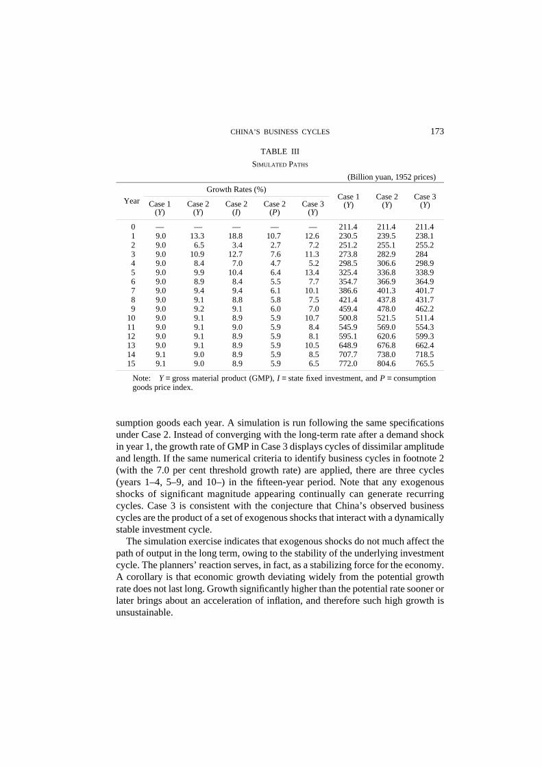
The first simulation, Case 1, is designed to draw the sustainable, or constant-rate-of-inflation, growth path by suppressing the cycles. To do so, state fixed in-vestment for each year is set to the level that keeps the rate of inflation at the meanof the 1979–92 period (6.0 per cent). The trajectory of GMP in Case 1 roughlyindicates the long-term stable growth path, around which output fluctuates in theshort term. The mean GMP (Y) growth rate over the fifteen-year period in Case 1,reported in Table III, is 9.0 per cent. This appears to indicate that China’s potentialgrowth rate since the late 1970s has been around 9 per cent.
For Case 2, a demand shock, which raises the growth rate of state fixed invest-ment by an additional 10 per cent in year 1, is inserted to activate the investmentcycle. The growth rates of GMP and state fixed investment and the rate of inflation(Table III, Case 2: Y, I, and P) exhibit a series of two-year cycles after the initialdemand shock. The amplitude of the cycles, however, falls rapidly, and the growthrates converge with their long-term trends, suggesting that the investment cycle inChina is dynamically stable. Case 2 appears to indicate, as economists generallybelieve, that a demand shock does not much alter the long-term growth path ofoutput. The difference between Cases 1 and 2 in the end point GMP (year 15, 772.0and 804.6 billion yuan) is relatively small. This finding also applies to a supplyshock. Inclusion of a single-year supply shock, in the form of a reduction of con-sumption goods output, in a simulation does not change output substantially in thelong term.
Because the Chinese economy is continually subject to exogenous shocks, whatone actually observes is a series of recurring cycles of varying magnitude andlength. In Case 3, to investigate how the dynamically stable investment cycleabove interacts with a succession of random shocks, a proxy variable for the vari-ability of climatic conditions is included in the model to alter the output of con-
––––––––––––––––––––––––––ment, household self-consumption, household consumption through payment in kind, non-house-hold consumption, and net exports.
173CHINA’S BUSINESS CYCLES
TABLE III
SIMULATED PATHS
(Billion yuan, 1952 prices)
Growth Rates (%)
Case 1 Case 2 Case 2 Case 2 Case 3(Y) (Y) (I) (P) (Y)
0 — — — — — 211.4 211.4 211.41 9.0 13.3 18.8 10.7 12.6 230.5 239.5 238.12 9.0 6.5 3.4 2.7 7.2 251.2 255.1 255.23 9.0 10.9 12.7 7.6 11.3 273.8 282.9 2844 9.0 8.4 7.0 4.7 5.2 298.5 306.6 298.95 9.0 9.9 10.4 6.4 13.4 325.4 336.8 338.96 9.0 8.9 8.4 5.5 7.7 354.7 366.9 364.97 9.0 9.4 9.4 6.1 10.1 386.6 401.3 401.78 9.0 9.1 8.8 5.8 7.5 421.4 437.8 431.79 9.0 9.2 9.1 6.0 7.0 459.4 478.0 462.2
10 9.0 9.1 8.9 5.9 10.7 500.8 521.5 511.411 9.0 9.1 9.0 5.9 8.4 545.9 569.0 554.312 9.0 9.1 8.9 5.9 8.1 595.1 620.6 599.313 9.0 9.1 8.9 5.9 10.5 648.9 676.8 662.414 9.1 9.0 8.9 5.9 8.5 707.7 738.0 718.515 9.1 9.0 8.9 5.9 6.5 772.0 804.6 765.5
Note: Y = gross material product (GMP), I = state fixed investment, and P = consumptiongoods price index.
Year Case 2(Y)
Case 1(Y)
Case 3(Y)
sumption goods each year. A simulation is run following the same specificationsunder Case 2. Instead of converging with the long-term rate after a demand shockin year 1, the growth rate of GMP in Case 3 displays cycles of dissimilar amplitudeand length. If the same numerical criteria to identify business cycles in footnote 2(with the 7.0 per cent threshold growth rate) are applied, there are three cycles(years 1–4, 5–9, and 10–) in the fifteen-year period. Note that any exogenousshocks of significant magnitude appearing continually can generate recurringcycles. Case 3 is consistent with the conjecture that China’s observed businesscycles are the product of a set of exogenous shocks that interact with a dynamicallystable investment cycle.
The simulation exercise indicates that exogenous shocks do not much affect thepath of output in the long term, owing to the stability of the underlying investmentcycle. The planners’ reaction serves, in fact, as a stabilizing force for the economy.A corollary is that economic growth deviating widely from the potential growthrate does not last long. Growth significantly higher than the potential rate sooner orlater brings about an acceleration of inflation, and therefore such high growth isunsustainable.

174 THE DEVELOPING ECONOMIES
VI. CHRONOLOGICAL REVIEW
I have reconstructed the nine business cycles with economic and statistical refer-ences.26 This review represents a reinterpretation of the cycles based on the ex-planatory framework. Some of the statistical series mentioned are found in Table I.The economic growth rates cited are based on NMP unless stated otherwise.
First cycle (–1957): upswing, –1956; downturn, 1957The government drafted an ambitious annual economic plan in 1956 after a good
harvest in 1955. State fixed investment in 1956 grew by 54.2 per cent, reflecting inpart the rapid expansion of the state sector following the nationalization drive ofindustry and commerce that year. In April, the government raised the wages ofstate sector workers by an average of 14.5 per cent [2, p. 173]. The high 1956growth target for gross agricultural output (11.5 per cent) was not fulfilled (actualgrowth, 5.0 per cent).27 Serious shortages of consumption goods appeared in theurban areas in the autumn. The government balanced the budget by reducing capi-tal construction expenditures, lowered output targets, and restrained new hiring inthe state sector in 1957. Pressures in the consumption goods market had receded,and currency in circulation had fallen by the end of 1957.
Second cycle (1958–62): upswing, 1958–59; downturn, 1960–62Under the Great Leap Forward from 1958, the government promoted an expan-
sion of fixed investment and industrial production centered on heavy industry, andit reorganized agricultural cooperatives into communes. State sector employmentgrew from 24.5 million in 1957 to 45.3 million in 1958, and budgetary appropria-tions for capital construction almost tripled during the 1958–60 period (1957, 12.4billion yuan; 1960, 35.4 billion yuan).28 Unfavorable weather resulted in poor har-vests for three consecutive years until 1961. The growth of industrial productiondecelerated as shortages of raw materials and energy became widespread. Themassive spending on fixed assets was slow to turn into new capacity because ofconstruction delays. The state budget marked record deficits in 1959 and 1960 (6.6and 8.2 billion yuan respectively) [19, 1993 ed., p. 215], and currency in circulationgrew by 138.1 per cent in the 1958–61 period [23, p. 349]. Food shortages resultedin famines in a number of regions around 1960. Faced with a crisis, the governmentcalled off the Great Leap Forward in the autumn of 1960 and initiated a retrench-
26 The references used are: [2] [4, various issues] [16, various issues] [17, various issues] [18] [19,various issues] [20, various issues] [23].
27 The target and actual growth rates are from [2, p. 162] and [19, 1984 ed., p. 132], respectively.28 State sector employment and budgetary appropriations for capital construction are from [19, 1993
ed., pp. 97, 222], respectively.
175CHINA’S BUSINESS CYCLES
ment program in 1961. Capital construction expenditures were cut back drasticallyto regain budgetary balance, and heavy industry was consolidated. Serious short-ages of daily necessities lasted long after the cancellation of the Great Leap For-ward. Real NMP at the trough (1962) declined to 64.8 per cent of the peak (1959)[19, 1993 ed., p. 34].
Third cycle (1963–68): upswing (1963–66); downturn (1967–68)The Chinese economy recovered from the deep recession by 1965, and the
economy was in an investment-led boom when the Cultural Revolution broke outin the spring of 1966. Disorder associated with intense political campaigns seri-ously affected industrial production, construction, and transportation from mid-1967 to early 1969. The revenue shortfall stemming from a sudden fall of industrialoutput (−13.8 per cent) generated a large and unexpected budgetary deficit (2.3billion yuan) in 1967 [19, 1993 ed., pp. 215, 413]. While industrial output contin-ued to fall (−5.0 per cent), gross agricultural output also dropped (−2.5 per cent),mainly because of poor weather conditions in 1968 [19, 1993 ed., p. 413] [19, 1984ed., p. 132]. Acute shortages of non-staples appeared that year. State fixed invest-ment declined by a large margin after a drop in 1967 (billion yuan: 1966, 25.5;1967, 18.8; 1968, 15.2), owing to retrenchment as well as to the disruptive effect ofthe Cultural Revolution [19, 1993 ed., p. 149]. The state budget was balanced in1968. The NMP declined two years in a row (1967, −7.2 per cent; 1968, −6.5 percent).
Fourth cycle (1969–72): upswing, 1969–71; downturn, 1972The recovery from the recession marked the beginning of a new round in the
industrialization drive. In the 1970–71 period, budgetary appropriations for capitalconstruction and new hiring in the state sector exceeded their initial targets by largemargins. Budgetary appropriations for capital construction in 1970 and 1971 were,respectively, 29.8 and 31.0 billion yuan [19, 1993 ed., p. 222], as against the targetsof 21.2 and 27.0 billion yuan [2, pp. 469, 486]. While the initial plan for new hiringwas 3.1 million during the two years, the number of state sector workers actuallyincreased by 9.8 million [2, p. 490]. Although rising demand pressures in the con-sumption goods market were partly offset by a good grain harvest in 1971, thegovernment imposed a mild restraint on fixed investment and new hiring in 1972.A poor harvest in 1972 also contributed to the deceleration of economic growththat year (2.9 per cent).
Fifth (1973–74) and sixth (1975–76) cycles: upswing, 1973 and 1975; downturn,1974 and 1976
These were back to back two-year cycles in the latter half of the Cultural Revo-lution period. China went through continual political campaigns in this period as

176 THE DEVELOPING ECONOMIES
various groups vied for post-Mao leadership. Disruption of economic order associ-ated with the “Anti-Lin, Anti-Confucius” campaign adversely affected industrialproduction (growth rate of gross industrial output, 0.6 per cent [19, 1993 ed.,p. 413]) and put an end to the fifth cycle in 1974. The downturn phase of the sixthcycle, 1976, was an eventful year. In view of the outbreak of yet another politicalcampaign organized by party radicals, government planners laid down modestgrowth targets for gross industrial (8.2 to 9.0 per cent) and agricultural (4 per cent)output [2, p. 555]. A powerful earthquake in July left the North China industrialand mining heartland paralyzed for some months. In October, a month after thedeath of Mao, the moderate wing of the party, which had secured power, an-nounced the ending of the Cultural Revolution. Gross industrial (1.3 per cent) andagricultural (2.5 per cent) output fell far short of the targets; the economic growthrate turned negative (−2.7 per cent), and the state budget ran a sizable deficit (3.0billion yuan) in 1976 [19, 1993 ed., pp. 215, 413] [19, 1984 ed., p. 132]. Shortagesof some major consumption goods were reported in 1974 and 1976 [2, pp. 532,561].
Seventh cycle (1977–81): upswing, 1977–79; downturn, 1980–81The ending of the Cultural Revolution brought back order in work places
throughout the nonagricultural sectors. In early 1978, after an economic recovery,the government announced a Ten-Year Economic Program which called for a si-multaneous expansion of major productive sectors through massive modernizationinvestment. The plan was soon abandoned because of its failure to address eco-nomic systemic problems. The party made a decision to launch economic reformsinstead in December 1978, the major contents of which were decentralization ofeconomic administration, wider use of markets, partial liberalization of privatebusiness activities, and promotion of foreign trade. Reform measures were adoptedstep by step from 1979. Some of the initial policies adopted, such as wage in-creases, hikes in purchasing prices of agricultural products, and reductions in agri-cultural taxes, forced the government to run large budgetary deficits in 1979 (17.1billion yuan) and 1980 (12.8 billion yuan) [19, 1993 ed., p. 215]. Because most ofthe deficits were covered by borrowing from the central bank, currency in circula-tion grew rapidly (1979, 26.3 per cent; 1980, 29.3 per cent). Inflationary pressures,however, stayed at manageable levels thanks to good harvests in 1978 and 1979and some new government measures; it began issuing treasury bonds, promotedsavings deposits with high interest rates, and directed resources to consumptiongoods industries to assist their output expansion. State fixed investment was cur-tailed in 1981, and the economy experienced a mild recession from 1980 (eco-nomic growth rate, 6.4 per cent) to 1981 (4.9 per cent).
177CHINA’S BUSINESS CYCLES
Eighth cycle (1982–89): upswing, 1982–88; downturn, 1989Decentralization of investment decision making under economic reforms
brought about successive increases of investment financed by internal reserves andstate bank loans. An investment-led boom began in 1982 and continued through1985. Decollectivization in agriculture and the adoption of the contract responsi-bility system resulted in sizable growth in agricultural output and rural householdincomes until 1984. As regulations on wages and bonuses in the state sector wererelaxed, cash incomes of urban households also grew at high rates.29 Inflationarypressures rose significantly by early 1985. The government restrained bank lendingto curb investment spending from the second half of 1985. The contractionarypolicy was terminated in the first half of 1986, before the rate of inflation droppedto low levels comparable to those of past disinflationary periods. A vigorous eco-nomic expansion led mainly by private consumption began with this relativelyhigh rate of inflation. Inflationary pressures rose from the spring of 1987 andpeaked in the summer of 1988. Although most of the pressures found their way intorising prices, shortages appeared in some daily necessities and consumer durablesin major cities around the summer of 1988. Having recognized that inflation was atits most serious since the early 1960s, the government implemented a strongcontractionary policy from the fall of 1988 to the spring of 1990. State banks re-stricted lending across the board, and state fixed investment was curtailed by fiat orsuasion. As the economy went into a recession, inflationary pressures receded.
Ninth cycle (1990–): upswing 1990–After a slow recovery, the Chinese economy was in the early stage of a boom
when Deng Xiaoping proposed the acceleration of economic growth in the springof 1992. A powerful investment boom followed immediately; state fixed invest-ment grew by 26.1 per cent in 1992 and by 14.7 per cent in 1993. This brought thestate fixed investment share of GDP to a very high level by 1993 (22.2 per cent),and the economic growth rate (as measured by GDP) reached 14.2 per cent in 1992and 13.5 per cent in 1993 [19, 1995 ed., p. 32]. High growth brought about acceler-ating inflation and a deteriorating trade balance. The rate of inflation (as measuredby the retail price index) grew from 2.9 per cent in 1991 to 13.2 per cent in 1993[19, 1995 ed., p. 233]. The trade balance moved from a surplus in 1992 (U.S.$4.4billion) to a deficit in 1993 (−U.S.$12.2 billion), reflecting the surge in imports [19,1995 ed., p. 537].
29 The wage reforms in the mid-1980s allowed state enterprises to set wages independently as long asthe growth of wages was linked to the indexes of enterprise performance. Decentralization of wagesetting resulted in fast increases of nominal wages in the state sector. The growth of wage costs aswell as expanding aggregate demand brought about the two most recent inflationary spells (1987–88 and 1992–94). Accounting for the dynamics behind the wage-cost inflation in the past decade isbeyond the scope of this article. See Imai [9] for further discussion.

178 THE DEVELOPING ECONOMIES
Reacting to these signals of rising macroeconomic pressure, the governmentimposed a mild contractionary policy in mid-1993 which included restraint onbank lending and state sector spending and interest rate hikes. Control over thegrowth of state bank loans was tightened successively in the following two years tolessen the growth of fixed investment and wage payments, and the yuan exchangerate was devalued from 5.8 to 8.7 yuan (official rate per U.S.$) in January 1994.Economic growth decelerated in 1994 (GDP, 11.8 per cent) [19, 1995 ed., p. 32] asthe growth rate of state fixed investment fell (10.3 per cent), and the trade balancemoved to a surplus the same year (U.S.$5.4 billion) [19, 1995 ed., p. 537]. Theimpact of contractionary policy on inflationary pressures in the retail market was,however, slow to appear. The rate of inflation peaked in 1994 (retail price index,21.7 per cent) [19, 1995 ed., p. 233] before dropping significantly in 1995 (Janu-ary–November, 15.4 per cent) [17, December 12, 1995]. Deng’s 1992 growth ac-celeration policy appears to have served as a demand shock that amplified the ninthcycle.
VII. CONCLUSION
The Chinese economy has experienced sizable short-term fluctuations of aggregateoutput in the past forty-one years since 1955. Nine business cycles can be identifiedbased on the growth rate of NMP during this period. There are common patterns,such as investment cycles, harvest fluctuations, and periodic retrenchments, whichsuggest the presence of some mechanisms for China’s business cycles. Anothernotable feature is the relative macroeconomic stability of the post-1979 periodcompared with the preceding period. My explanatory framework is that China hasan investment cycle of the kind described by Kornai’s hypothesis, and that thiscycle interacts with exogenous shocks and generates business cycles of dissimilaramplitude and duration. According to Kornai, an investment cycle is generated bythe patterned reaction of central planners who adjust the level of fixed investmentin response to capacity pressure, an indicator of macroeconomic tension. An insti-tutional prerequisite of this cycle is the weak financial accountability of state enter-prises, which results in the upward drift of state fixed investment. My survey hasindicated that the Chinese economy, seventeen years after the initiation of eco-nomic reforms, still has an investment cycle with these characteristics. The rate ofinflation being an indicator of macroeconomic tension, state fixed investment andthe rate of inflation move in tandem in China’s investment cycle. The exogenousshocks in the post-1979 period as a set seem to have been less destabilizing to theeconomy than those in the preceding period, and this may partly explain the rela-tive macroeconomic stability of the past seventeen years.
The dynamic simulation performed, based on the data since the late 1970s, indi-cates that the underlying investment cycle in China is dynamically stable. Because
179CHINA’S BUSINESS CYCLES
of this stability, an exogenous shock has little effect on the long-term growth pathof output. China’s potential growth rate in the reform period appears to be around 9per cent. The simulation results also indicated that a series of random shocks, suchas those associated with climatic variation that affect agricultural output, couldproduce recurring output cycles of different amplitude and length. Chronologicalaccounts appear to show that economic developments during the past nine businesscycles were largely consistent with the explanatory framework presented.
Will ongoing economic reforms alter the pattern of China’s business cycles? Inthe long term, rapidly expanding non-state sectors may reduce the state sector to asmall segment of the economy. Then the peculiarities in state enterprise investmentbehavior will no longer significantly affect the patterns of output fluctuations. InNovember 1993 the Communist Party stopped short of accepting the state sector’sdecline into irrelevance and announced that the government would graduallyimplement banking and taxation reforms and promote the introduction of privatefunds into state enterprises over the coming years [1, pp. 14–21]. As reforms pro-ceed, it is conceivable that state enterprises will eventually assume full financialaccountability or be privatized. Also, state banks will begin to act as independentcommercial banks, applying objective economic criteria in lending. At that point,state enterprises will lose their bias for expansion and the pattern of business cycleswill change.
REFERENCES
1. Central Committee of the Chinese Communist Party. “Decision of the CPC CentralCommittee on Some Issues concerning the Establishment of the Socialist Market Eco-nomic Structure,” Beijing Review, Vol. 36, No. 47 (November 1993).
2. CHEN JIDONG, LI RUOYU, and GAO HONGFANG, eds. Zhonghua renmin gongheguo jingjidashiji, 1949–1980 [Major economic events of the People’s Republic of China, 1949–1980] (Beijing: Zhongguo-shehui-kexue-chubanshe, 1984).
3. CHEN JINHUA. “Report on the Implementation of the 1994 Plan for National Economicand Social Development and the Draft 1995 Plan for National Economic and SocialDevelopment,” Beijing Review, Vol. 38, Nos. 14–15 (April 1995).
4. China Daily.5. DING HENGJIANG and LIU XIAOQI. “Guanyu difang zhengfu ganyu yinhang jingying
huodong di shenceng sikao” [Deep thoughts on intervention by local governments inthe operational activities of banks], Jingji yanjiu, No. 12 (1993).
6. ECKSTEIN, A. “Economic Fluctuations in Communist China’s Domestic Develop-ment,” in China’s Heritage and Communist Political System, ed. Ho Ping-ti and TangTsou, Vol. 2 (Chicago: University of Chicago Press, 1968).
7. FAN GANG, ZHANG SHUGUANG, and WANG LIMIN. “Shuanggui guodu yu shuangguidiaokong (I)” [Dual-track transition and dual-track macroeconomic management (I)],Jingji yanjiu, No. 10 (1993).
8. IMAI, H. “Inflationary Pressure in China’s Consumption Goods Market: Estimationand Analysis,” Developing Economies, Vol. 32, No. 2 (June 1994).

180 THE DEVELOPING ECONOMIES
9. ––––––––––. “Growth-Inflation Tradeoff in China,” Lingnan College, Centre forAsian Pacific Studies, Working Paper Series No. 25 (Hong Kong, 1995).
10. KORNAI, J. The Socialist System (Oxford: Clarendon Press, 1992).11. KORNAI, J., and DANIEL, Z. “The Chinese Economic Reform—As Seen by Hungarian
Economists,” Acta Oeconomica, Vol. 36, Nos. 3–4 (1986).12. MA HONG, ed. Modern China’s Economy and Management (Beijing: Foreign Lan-
guage Press, 1990).13. NAUGHTON, B. “Saving and Investment in China: A Macroeconomic Analysis”
(Ph.D. diss., Yale University, 1986).14. ––––––––––. “Macroeconomic Policy and Response in the Chinese Economy: The
Impact of the Reform Process,” Journal of Comparative Economics, Vol. 14, No. 3(September 1987).
15. ––––––––––. “Inflation in China: Patterns, Causes, and Cures,” in China’s EconomicDilemmas in the 1990s: The Problems of Reforms, Modernization, and Interdepen-dence, ed. Joint Economic Committee, U.S. Congress, Vol. 1, Compendium of Papers(Washington, D.C.: U.S. Government Printing Office, 1991).
16. Nihon keizai shimbun.17. Renmin ribao.18. State Statistical Bureau, ed. Zhongguo maoyi wujia tongji ziliao, 1952–1983 [Trade
and price statistics in China, 1952–1983] (Beijing: Zhongguo-tongji-chubanshe,1984).
19. ––––––––––. Zhongguo tongji nianjian [Statistical yearbook of China] (Beijing:Zhongguo-tongji-chubanshe, various years from 1984 to 1995).
20. Wall Street Journal.21. WONG, C. “The Economics of Shortages and Problems of Reform in Chinese Indus-
try,” Journal of Comparative Economics, Vol. 10, No. 4 (December 1986).22. WU NAITAO. “Risk Investment System to Be Established,” Beijing Review, Vol. 37,
No. 15 (April 1994).23. XU KANGHUA and WANG YAPING. Zhongguo shehui zhuyi jianshe xinshiqi jingji jianshi
[Short history of the new period of China’s socialist construction] (Beijing:Zhongguo-wuzi-chubanshe, 1993).
24. Zhongguo caizheng tongji (1950–1991) [China finance statistics (1950–1991)](Beijing: Kexue-chubanshe, 1992).
25. Zhongguo jingji nianjian, 1991 [Almanac of the China’s economy, 1991] (Beijing:Jingji-guanli-chubanshe, 1991).
26. Zhongguo jinrong nianjian, 1993 [Almanac of China’s finance and banking, 1993](Beijing: Zhongguo-jinrong-nianjian-bianjibu, 1993).
APPENDIX
MACROECONOMIC MODEL FOR DYNAMIC SIMULATION
A. Notation
Numerical subscripts with minus signs indicate past years (e.g., −1 denotes theprevious year). ∆ denotes the annual increment. Endogenous variables are repre-
181CHINA’S BUSINESS CYCLES
j
i=0
sented by capitals; exogenous variables are denoted by either lower case or Greekletters.Endogenous variables:
F = nominal savings deposit balances (year end).G = nominal household income (annual).I = state fixed investment in 1952 prices (annual).K = capital stock in the consumption goods industry in 1952 prices (year end).M = nominal currency supply (year end).P = price of consumption goods (annual mean, base year = 1952, 1952 level =
1).Q = output of consumption goods in 1952 prices (annual).Y = gross material product (GMP) in 1952 prices (annual).
Exogenous variables and coefficients:r = nominal interest rate on savings deposits.t = time trend (zero until 1978, 1979 = 1, 1980 = 2, . . . ).w = nominal annual wage rate.φa = labor productivity in the consumption goods industry.φb = labor productivity in the investment goods industry.γ = allocation ratio of new capital to the consumption goods industry.τ = rate of depreciation.ρ−i= distributed lags describing the pattern in which current and past years’ in-
vestment fully contributes to the expansion of capital stock. ρ0 is the weighton current year investment.
B. Equations
Q = αK−1, (1)α > 0, K > 0.
100・ = β1 + β2100・ , (2)
I > 0, β1 > 0, β2 < 0.
∆K = γ ∑ ρ−iI -i − τK−1, (3)
0 < γ < 1, ρ−i > 0, ρ0 + ρ−1 + . . . + ρ−j = 1, 0 < τ < 1.
G = α K−1 + I + r−1F−1, (4)
w > 0, φa > 0, φb > 0, r > 0, F > 0.
G = PQ + ∆M + ∆F , (5)P > 0.
II-1
( − 1) ( P-1
P-2
− 1 )
wφb
( )wφa
( )
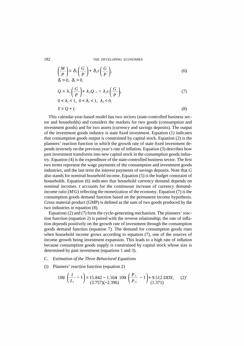
182 THE DEVELOPING ECONOMIES
= δ1 + δ2 t , (6)
δ1 > 0, δ2 > 0.
Q = λ 1 + λ 2Q−1 + λ 3t , (7)
0 < λ1 < 1, 0 < λ2 < 1, λ3 < 0.
Y = Q + I. (8)
This calendar-year-based model has two sectors (state-controlled business sec-tor and households) and considers the markets for two goods (consumption andinvestment goods) and for two assets (currency and savings deposits). The outputof the investment goods industry is state fixed investment. Equation (1) indicatesthat consumption goods output is constrained by capital stock. Equation (2) is theplanners’ reaction function in which the growth rate of state fixed investment de-pends inversely on the previous year’s rate of inflation. Equation (3) describes howpast investment transforms into new capital stock in the consumption goods indus-try. Equation (4) is the expenditure of the state-controlled business sector. The firsttwo terms represent the wage payments of the consumption and investment goodsindustries, and the last term the interest payments of savings deposits. Note that Galso stands for nominal household income. Equation (5) is the budget constraint ofhouseholds. Equation (6) indicates that household currency demand depends onnominal incomes. t accounts for the continuous increase of currency demand-income ratio (M/G) reflecting the monetization of the economy. Equation (7) is theconsumption goods demand function based on the permanent income hypothesis.Gross material product (GMP) is defined as the sum of two goods produced by thetwo industries in equation (8).
Equations (2) and (7) form the cycle-generating mechanism. The planners’ reac-tion function (equation 2) is paired with the reverse relationship; the rate of infla-tion depends positively on the growth rate of investment through the consumptiongoods demand function (equation 7). The demand for consumption goods riseswhen household income grows according to equation (7), one of the sources ofincome growth being investment expansion. This leads to a high rate of inflationbecause consumption goods supply is constrained by capital stock whose size isdetermined by past investment (equations 1 and 3).
C. Estimation of the Three Behavioral Equations
(i) Planners’ reaction function (equation 2)
100・ = 15.842 − 1.164・100・ + 9.512 DDX, (2)′II-1
( − 1) ( P-1
P-2
− 1 )(3.757)(−2.396) (1.371)
MP( ) G
P( ) GP( )
GP( ) G
P( )

183CHINA’S BUSINESS CYCLES
Adjusted R2 = 0.256, D.W. = 1.659, period = 1979–94.(Figures in parentheses are t-statistics.)
DDX, the dummy variable associated with the high growth policy proposed byDeng Xiaoping (1992, 1993, and 1994 = 1, zero in other years), is added as anexplanatory variable.
(ii) Currency demand function (equation 6)
= 0.123 + 0.009t , (6)′
Adjusted R2 = 0.994, D.W. = 1.905, period: 1978–92.
(iii) Consumption goods demand function (equation 7)
Q = 0.812 + 0.172Q−1 − 0.013t , (7)′
Adjusted R2 = 0.998, h = −0.528, period: 1978–92.
D. Numerical Assumptions
(i) Coefficients estimated above are used for equations (2), (6), and (7).(ii) Initial value of K−1: 250 billion yuan in 1952 prices. This is the assumption
on the size of the capital stock in the consumption goods industry in 1977. Usingequation (1), α (0.364) is obtained as the ratio of consumption goods output (Q) in1978 (91.0 billion yuan in 1952 prices) to capital stock (K) in 1977 (250 billionyuan).
(iii) r: 6.9 per cent through the period (mean interest rate on one-year savingsdeposits in the 1979–92 period).
(iv) w’s annual growth rate: 14.5 per cent (geometric mean growth rate in the1979–92 period).
(v) φa’s annual growth rate: 4.9 per cent (geometric mean growth rate in the1979–92 period).
(vi) φb’s annual growth rate: 8.2 per cent (geometric mean growth rate in the1979–92 period).
(vii) γ: 0.5.(viii) τ : 0.05.(iv) ρ−i: ρ0 = 0.4, ρ−1 = 0.3, ρ−2 = 0.2, ρ−3 = 0.1.
E. Simulation Setup
Case 1. Equation (2) is dropped, and P is set exogenously to grow by 6.0 percent a year through the simulation period. This is the growth rate of the consump-tion goods price index in the 1979–92 period. The seven equations determine the
MP( )
(17.356))G
P( )GP(
(14.122)
GP( )G
P( )(17.308) (3.228) (−12.359)

184 THE DEVELOPING ECONOMIES
values of seven endogenous variables recursively each year. Each of the sevenendogenous variables is associated with an equation: (1)-Q, (3)-K, (4)-I, (5)-F,(6)-M, (7)-G, (8)-Y. The simulation is run for nineteen years. The initial values ofendogenous variables are set at the 1977 level. Because it takes a few years beforeendogenous variables move smoothly, the observations in the first four years arediscarded and the fifth year is labelled as year 1 and the nineteenth as year 15.
Case 2. Case 2 uses the full eight-equation model. Each of the eight endog-enous variables is associated with an equation: (1)-Q, (2)-I, (3)-K, (4)-G, (5)-F,(6)-M, (7)-P, (8)-Y. An investment shock term, which adds another 10 per cent tothe growth rate of state fixed investment, is inserted in equation (2) in year 1. Thesimulation is run for fifteen years.
Case 3. A proxy variable that represents the variation in climatic conditions isincluded in equation (1) as a multiplicative term on the right-hand side. Otherspecifications are the same as in Case 2. The climatic variation variable is based onthe ratio of the crop acreage affected substantially by natural disasters to the totalsown area for the fifteen years from 1978 to 1992 [19, 1993 ed., pp. 358, 391]. Themean of this ratio is 0.132. Crop acreage affected substantially indicates the outputper area fallen by more than 30 per cent from the normal-year level [19, 1993 ed., p.391]. The percentage deviation of this ratio is divided by 15 to generate the seriesof the proxy variable. This implies, for the sake of simulation, that a 10 per cent risein the ratio from 0.132 to 0.145, reflecting poor climatic conditions, results in a0.67 per cent reduction in consumption goods output.
F. Description of the Data
F = savings deposits balances at the end of the year [19, 1993 ed., p. 285].I = state fixed investment (see Table I, source).M = nominal household currency balances [18, p. 8].P = consumption goods price index in the retail price index (see Table I,
source).Q = nominal value of household cash expenditures for consumption goods and
services divided by P [18, p. 14].a
r = mean annual interest rate on one-year savings deposits [26, p. 385].w = G net of interest payments (r−1F−1) divided by the number of employees at
the end of the year [19, 1993 ed., p. 97].φa and φb = computed using the numbers of workers in the two industries. The
number of workers in the investment goods industry is obtained by dividing
a Note that Q omits the bulk of the value of services consumed by households, because householdstypically pay only a small part of the costs of some services such as housing and health care inurban areas. This is why expenditures for services are very small relative to those for consumptiongoods. In 1992, household cash expenditures for services and goods were, respectively, 103.1 and862.1 billion yuan [19, 1993 ed., pp. 602, 611].

185CHINA’S BUSINESS CYCLES
nominal gross state fixed investment by w. The number of workers in theconsumption goods industry is obtained as the difference between the totalnumber or workers and the number of workers in the investment goods in-dustry.
G and Y = computed using equations (4) and (8).