1

P(E) = P(E ∩ A) + (E ∩ A’)

P(A ∩ B) = P(B ∩ A)

P(S) = P(A) + P(A’)

A ∩ A’ = Ǿ

and A U A’ = S

P(A ∩ B) = P(A | B) * P( B ) Explaining

Bayes Theorem

A Progression of Ideas Illuminating an

Important Mathematical Concept

By Dan Umbarger www.mathlogarithms.com

)(

)(*)|()|(

BP

APABPBAP

2

Foreword

When I did my undergraduate work it was “de rigueur” for computer science majors to also study

calculus in order to complement the training we were taking in the Computer Science. Additionally,

since all our professors were also mathematics teachers, we usually had assignments requiring knowledge

of math. As time went on Computer Science at the post high school level has pretty well separated from

mathematics and, at least for the non-engineer majors, requires less function based mathematics and more

discrete math and statistics. I do not wish to debate whether or not a high school student contemplating

a university computer science major should take calculus or statistics or discrete math. It is quite clear to

me that they should take as much mathematics as their high school offers.

One area of non-calculus based mathematics that has been increasingly used in artificial intelligence

applications of computer science is “probability based decision making.” High school teachers have

always taught decision making (if, if-else, switch-case) based upon randomly generated numerical values.

At the university and applied level we see decisions being made based upon more sophisticated

criteria…conditional probability. A major part of this work is predicated upon knowledge of Bayes’

Theorem. Bayes' Theorem is named after the Reverend Thomas Bayes of England, 1702-1761 (who

reportedly developed it while trying to prove the existence of God) although there is some evidence that a

Nicholas Saunderson, the blind Lucasian professor at Cambridge (think Sir Issac Newton and Stephen

Hawkings!!) actually discovered the principles that are generally credited to Rev. Bayes.

http://en.wikipedia.org/wiki/Nicholas_Saunderson

In Computer Science Bayes Theorem is used in enhancing low resolution imaging and in

filtering situations such as spam and noise filters…all situations involving “probability based

decision making.”

As a long time high school computer science teacher it occurs to me that such a powerful tool should

be made available to interested high school students. We all have students who are pushing beyond the

AP Computer Science curriculum and applications of Bayes Theorem would be a good topic for such a

student to investigate. It could possibly benefit them greatly after high school. As I was not able to

locate any high school age appropriate materials explaining Bayes Theorem I have determined to try to

fill the void. When I looked back at my university business stat book I found the standard Bayes

Theorem formulas given with no discussion or motivation or progression of ideas anywhere… a great

example of “Athena jumping out of the head of Zeus.” No wonder I never understood Bayes Theorem

while in university! My math stat book was too advanced for me and my business stat book was too

trivial and vague to understand…just magic formulas to manipulate and quickly forget after the unit test

Hopefully I have sailed between Scylla and Charybdis here.

By traditional standards I am not particularly qualified to undertake this task but in a strange way

that makes me even more suited to such a task. I noticed some time ago that many (most) of those

people for whom abstract ideas come easily cannot communicate well with others who do not have

similar background and/or ability. Many (most) of my high school computer geniuses can jibber-jabber

up a storm with their intellectual equals but are totally ineffective in trying to communicate with less

capable classmates. My struggle to master concepts usually results in developing visuals. Those

visuals achieve two goals. They allow my brighter students to master the material even more quicker

than ever while still providing access of ideas to those less academically gifted students who still need or

could benefit from the material.

3

Table of Contents

Page

Chapter 1, Bayes Theorem, An Anticipatory Set……………………….. 4

Chapter 2, Bayes Theorem, An Informal Derrivation……………………. 6

Chapter 3, Bayes Theorem, Applied, No Grid…………………………... 13

Chapter 4, Extended Bayes Theorem…………………………………….. 15

4

Chapter 1, Bayes Theorem, An Anticipatory Set

In the educational world an “anticipatory set” is a preliminary discussion of a topic that introduces

ideas and vocabulary and “sets the stage” so to speak for what is to come. It gives the student the “big

picture” before proceeding to work with the details.

Problem: A given population is 40% male and 60% women. 30% of the males like to fish but only

10% of the females like to fish. A visual can make all this data immediately available to

our brains to process.

List all the probabilities this data

suggests. Several are obvious

from the figure.

Probability a person chosen at random from set P is male, P(male) = 40% of entire population

Probability a person chosen at random from set P is female, P(female) = 60% of entire population

Probability of picking at random from set of males a subject who likes to fish:

P(fish | male) = 30% of males… given… duh! ( but 30% * 40% = 12% of entire population)

Probability of picking at random from the set of females a subject who likes to fish:

P(fish | female) = 10% of females... given … duh! (but 10% * 60% = 6% of entire population)

Notice the symbolism P(fish | male) and P(fish | female).

P(fish | male) is read as “the probability of choosing a person who likes to fish from the set of males.”

P(fish | female) is read as “the probability of choosing a person who likes to fish from the set of females.”

Probabilities of the form P(set 1 | set 2) are called “conditional probabilities.”

Question: What would be the probability of randomly chosing a male from the set of people who like to

fish? Symbolically this would be P(male | fish) = ?

It was pretty easy to ascertain P(fish | male). (30% of males but 30%*40% = 12% of entire population)

It is not so easy to ascertain P(male | fish). That is what learning Bayes Theorem will enable you to do.

Notice that the values P(fish | male)

and P( male) are readily available

from the given data but value

P(male | fish) and P(fish) are not!

5

Suppose the original problem was changed as follows:

Problem: In a given population are 40 males and 60 female. 30% of the males like to fish but only

10% of the females like to fish. A visual can make all this data immediately available to

our brains to process.

Here we have cardinal numbers for our gender data rather than percentages. Again list all the

information that this data implies.

What % of the males like to fish? … 30% What % of the females like to fish?... 10%

What % of the population is male?...40/100. What % of the population is female?...60/100.

How many males are there in the population? … 40. How many females are in the population?…60

How many males like to fish? 30% * 40 = 12 How many females like to fish? 10% * 60 = 6

This new data can be calculated from the given data.

Given that a person is chosen at random from

the set of people who like to fish what is the

probability that that person is a male? P(male | fish).

Although slightly disguised this is same situation

as posedon the previous page and is the kind of

problem that Bayes theorem will allow us to solve.

(Note that if #male + #female ≠ 100 we could use

the given counts and calculate %.)

6

(A ∩ B) = (B ∩ A)

)(

)(*)|()|(

fishP

malePmalefishPfishmaleP

Chapter 2, Bayes Theorem, An Informal Derrivation

Where in the world does Bayes

Theorem come from? How do we

know that it works? Smart university

math teachers are more than eager to

derrive this theorem. Even if I knew

how to derrive this theorem it would not be appropriate to do so in materials which are being targeted to

high school students. What follows is considered an informal, non-rigorous, intuitive, demonstration

which will appropriately serve to create a familiarity with and a confidence in Bayes Theorem.

We start by learning (or reviewing) a

basic rule in set theory…

The Commutative Property of Interesection

The figures below seem to support this idea. We could use a truth table but it seems unnecessary.

Another basic rule from set theory which we will need and you should recognize from Geometry is that

the “whole is equal to the sum of its parts.” In the figure shown below set X = set E U set E’ .

Notice that this rule only works if the parts are mutually exclusive and entirely partition set X.

X

7

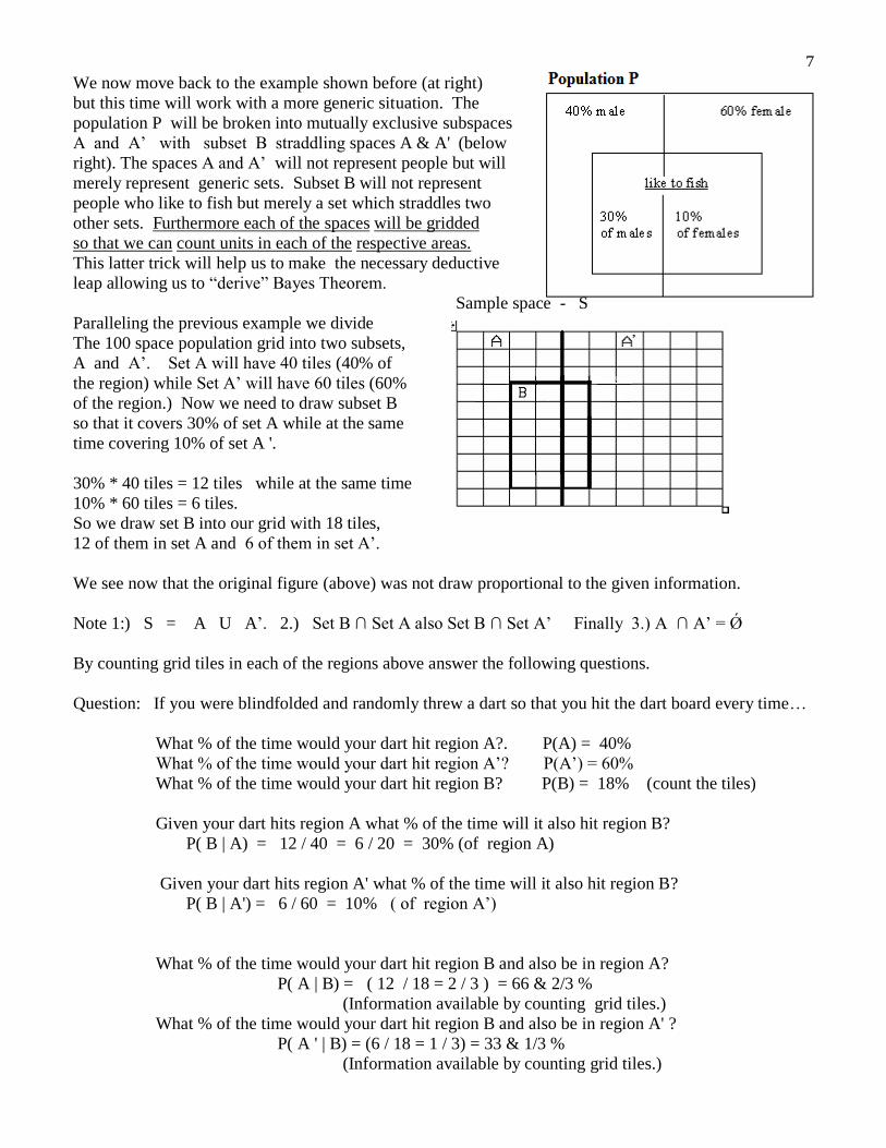
We now move back to the example shown before (at right)

but this time will work with a more generic situation. The

population P will be broken into mutually exclusive subspaces

A and A’ with subset B straddling spaces A & A' (below

right). The spaces A and A’ will not represent people but will

merely represent generic sets. Subset B will not represent

people who like to fish but merely a set which straddles two

other sets. Furthermore each of the spaces will be gridded

so that we can count units in each of the respective areas.

This latter trick will help us to make the necessary deductive

leap allowing us to “derive” Bayes Theorem.

Sample space - S

Paralleling the previous example we divide

The 100 space population grid into two subsets,

A and A’. Set A will have 40 tiles (40% of

the region) while Set A’ will have 60 tiles (60%

of the region.) Now we need to draw subset B

so that it covers 30% of set A while at the same

time covering 10% of set A '.

30% * 40 tiles = 12 tiles while at the same time

10% * 60 tiles = 6 tiles.

So we draw set B into our grid with 18 tiles,

12 of them in set A and 6 of them in set A’.

We see now that the original figure (above) was not draw proportional to the given information.

Note 1:) S = A U A’. 2.) Set B ∩ Set A also Set B ∩ Set A’ Finally 3.) A ∩ A’ = Ǿ

By counting grid tiles in each of the regions above answer the following questions.

Question: If you were blindfolded and randomly threw a dart so that you hit the dart board every time…

What % of the time would your dart hit region A?. P(A) = 40%

What % of the time would your dart hit region A’? P(A’) = 60%

What % of the time would your dart hit region B? P(B) = 18% (count the tiles)

Given your dart hits region A what % of the time will it also hit region B?

P( B | A) = 12 / 40 = 6 / 20 = 30% (of region A)

Given your dart hits region A' what % of the time will it also hit region B?

P( B | A') = 6 / 60 = 10% ( of region A’)

What % of the time would your dart hit region B and also be in region A?

P( A | B) = ( 12 / 18 = 2 / 3 ) = 66 & 2/3 %

(Information available by counting grid tiles.)

What % of the time would your dart hit region B and also be in region A' ?

P( A ' | B) = (6 / 18 = 1 / 3) = 33 & 1/3 %

(Information available by counting grid tiles.)

8

Gathering together all the observations from the bottom of pg. 7

P( A ) = 40%, P( A’ ) = 60%

P( B ) = 18%

P( B | A) = 30%, P( B | A' ) = 10%

P( A | B) = 2 / 3 ( 2/3 of B grids are in A)

P( A' | B) = 1 / 3 (1/3 of B grids are in A' )

A ∩ B = 12 tiles so P(A ∩ B) = 12/100 = 12 %

A' ∩ B = 6 tiles so P(A' ∩ B) = 6/100 = 6 %

The next part is guarenteed to cause a university mathematics professor to cringe. There is a relation

among the different probability values shown above.

P(A ∩ B ) = 12%, P( A | B) = 2 / 3, and P( B) = 18%

12% = (2 / 3) * 18%

P(A ∩B) = P(A | B) * P(B) *** special equation #1

Also there is a relation among the following probability values

P( B ∩ A ) = 12%, P( B | A) = 30%, and P( A) = 40%

12% = 30% * 40%

P( B ∩ A ) = P( B | A) * P( A ) *** special equation #2

All the pieces are now in place….

P(A ∩B) = P( B ∩ A ) commutative property of intersection

P(A | B) * P(B) = P(A ∩B) = P( B ∩ A ) = P( B | A) * P( A ) ** special eqs. #1 & 2

Thus by transitive P(A | B) * P(B) = P( B | A) * P( A )

Hence

Ta da !

P(A | B) = P( B | A) * P( A )

P( B )

9

)(

)(*)|()|(

fishP

malePmalefishPfishmaleP

Recopying from previous page.

This is what we wanted… an expression for what we do not know in terms of what we do know (or can

find out). In the derrivation of this formula we knew P(A | B) to be 2 / 3 because we had access to grid

tiles and could count them to come up with 12 / 18 which is the probability that a value is in set A given

that it is in set B. Likewise P(B) = 18%... we counted Set B grid tiles to get the 18 (12 + 6) . However

this example is a contrived one utilizing a grid with countable squares which is not usually going to be the

case. In general you will only be able to access P(B | A) and P( A ). You will have to use a formula to

access P( A | B) and P( B).

If this paragraph did not make sense take a

moment to review the data at right.

P (like to fish given you are male) = P( fish | male) = 30% of male

(given) or (30% * 40%) = 12% of entire population

P ( male ) = 40 / 100 (given)

P (likes to fish) = ??? … cannot do without a grid or a formula.

[It is not 30% + 10%, but rather cardinality(30%) + cardinality(10%) ]

cardinality(population)

P (someone chosen from the set of fishophiles is a male) = ???

[It is not (30% + 10%)/40%, stay tuned… this is coming.]

Lets compare this new formula with the one given several pages back on pages 4 & 6.

Now if only we could determine P( B ) (or P(fish) without a grided figure we would have everything

necessary to calculate P( A | B).

Clearly P( B ) below is 18 / 100 = 18% However P(like to fish) is not clear.

by counting grid tiles. (or (8 + 12) / 100 ) It is not 30% + 10% !!!

P(A | B) = P( B | A) * P( A )

P( B )

P(A | B) = P( B | A) * P( A )

P( B )

10

A basic rule from set theory which you should recognize from Geometry is that the whole is equal to the

sum of its parts. In the figure shown below set X = set E U set E’ . Notice that this rule only

works if the parts are mutually exclusive and entirely partition set X.

X

Therefore P( X ) = P( E ) + P( E ' )

Previously P(B) = 12 / 100 + 6 / 100

= 18 / 100

Without the grid tiles n the figure at right,

but using the special equation 2 (pg 8)

P( B ∩ A ) = P( B | A) * P( A ) *** special equation #2, pg. 8

we can obtain P(B) as follows.

P(B) = [(A ∩ B) U (A' ∩ B)]

= [ (B ∩ A) U (B ∩ A' ) ]

= { [ P(B | A) * P (A) ] U [ P(B | A' ) * P(A') ] } … special equation #2, applied twice

= [ (0.30 * 0.40) + [ 0.10 * 0.60 ]

= ( 0.12 + 0.06)

= 18 % This works as expected from the grid count

because we are adding cardinalities here not %’s (30% + 10% ≠ 18% )

For the figure at right

Probability that someone chosen at random

from the entire set of data who likes fish is:

P(like to fish) = P(male and like to fish)

+

P(female and like to fish)

= 30% * 40% + 10% * 60%

= 12% + 6%

= 18% (no counting of grid tiles)

11

P(A | B) = P( B | A) * P( A )

P( B )

P(A | B) = ____P( B | A) * P( A )________ (probability of interest)____

P(B |A)*P(A ) + P(B |A ' )*P( A ' ) (probability of either event

occuring

P(male | fish) = ___ _P( fish | male) * P( male )____________

P(fish |male)*P(male ) + P(fish |female)*P( female )

= ____30% * 40%____ = 12%__ = 12% = 2

30%*40% + 10%*60% 12% + 6 % 18% 3

= which we got previously by counting grid tiles (pg. 10)

i.e. P(male | fish) = probability a male who likes to fish is chosen from the set of males

probability of chosing at random from all those who like to fish

Thus for a sample space subdivided into two mutually exclusive partitions

with A U A' completely filling the sample space

Bayes Theorem

However since

P(B) = ( B ∩ A) U ( B∩A' ) or using special equation 2 from pg. 8 P( B ∩ A ) = P( B | A) * P( A )

P( B) = [ P(B | A) * P (A)] U [P( B | A ' ) * P(A ' ) ] *** spec. eq. #2 applied twice on both A and A '

The later P(B) form indicates that the probability of B happening is equal to the sum of the

probability of B happening given A + the probability of B happening given A '

Subistituting for P(B) in the denomimator Bayes Theorem can now be rewritten as

or for the fish problem on page 10

12

A caveat. The reason that college math professors would object to this treatment of Bayes Theorem

is that I have taken a sample of size one and used it to deduce a general rule. Induction is actually a

commonly used and accepted technique by mathematicians but not in its limited form as shown here.

Specifically I have inductively concluded that

P( A ∩ B) = P( A | B) * P( B ) and

P( B ∩ A ) = P( B | A) * P( A )

based upon a sample of size one. In the world of mathematics that is not enough evidence to make a

generalized conclusion. This paper, however, is not written for mathematicians but for high school

students. Unlike the business and psych stat books I had in college it at least tries to motivate and

explain where Bayes Theorem comes from.

13

P(A | B) = P( B | A) * P( A )

P( B )

P(A | B) = ____P( B | A) * P( A )________

P(B |A)*P(A ) + P(B |A' )*P( A' )

P(S | TP) = ____P( TP | S) * P( S )________

P(TP |S)*P(S ) + P(TP | S ' )*P( S ' )

P(S | TP) = P( TP | S) * P( S )

P( TP )

Chapter 3, Bayes Theorem, Applied…No Grid

When doing an experiment there are four things that can happen. The experiment can:

1.) correctly identify something as true (correct true test)

2.) incorrectly identify something as true (false positive)

3.) correctly identify something as false (correct false test)

4.) incorrectly identify something as false (false negative)

For example. Suppose there was a drug test that was developed to test atheletes for use of steroids.

It is not a 100% accurate test. Sometimes:

1.) it correctly identifies an athelete as being a drug user (true positive)

2.) it incorrectly identifies an athelete as being a drug user (false positive)

3.) it correctly concludes that an athelete does not use a drug (true negative)

4.) it incorrectly concludes that an athelete does not use a drug (false negative)

A manufacturer claims that its test for steroids results in 95% true positives and 15% false positives.

10% of the team uses steroids. Your teammate just tested positive. What is the probability that your

friend uses steroids? Let S represent those atheletes on your team that use steroids. Hence S ' will

be those atheletes that do not use steroids. Let TP represent all the people who test positive for

steroids… TestPositive = true positive + false positive

Your teammate just tested positive. What is the

probability that your friend is a user?

You are to calculate P( S | TestPositive)

Let TP = TestPositive (true positive + false positive)

The generic Bayes theorems are:

For this specific problem the formulas would be:

14

P(S | TP) = P( TP | S) * P( S )

P( TP )

P(S | TP) = ____P( TP | S) * P( S )________

P(TP | S)*P(S ) + P(TP | S ' )*P( S ' )

P(A | B) = P( B | A) * P( A )

P( B )

P(A | B) = ____P( B | A) * P( A )________

P(B |A)*P(A ) + P(B |A’)*P( A )

Putting everything together now

A manufacturer claims that its test for steroids results in 95% true positives and 15% false positives.

10% of the team uses steroids. Your teammate just tested positive. What is the probability that your

he/she uses steroids?

Let S represent those atheletes on your team that use steroids. Hence S ' will be those atheletes that

do not use steroids. Let TP represent all the people who test positive for steroids…

TP = true positive + false positive

Your friend just tested positive. What is the

probability that your friend is a user?

Given: P(S) = 10%

P(TP | S) = 95%

P(TP | S ' ) = 15%

Implied: P(S ' ) = 90%

The generic Bayes Theorems are:

For this specific problem the formulas would be:

P(S | TP) = ______95% * 10%___

(95% * 10%) + (15% * 90%)

= 0.095

0.23

= 0.413

= 41% probability that friend uses steroids

15

Chapter 4, Extended Bayes Theorem

Recall from the original example that the sample space was split into two mutually exclusive

subspaces.(See fig. below left.) Bayes Theorem can be extended to apply to those situations where the

subspace is split into more than two subspaces (See fig. below right) as long as the subspaces completely

partition the original space and the subspaces are mutually exclusive. Notice in the fig. at right that

% French + % British + % American = 100%. Assume that there are no subjects with dual citizenship.

What is the probability of picking a person at random from the population of French, British, and

American suggested above and

picking a French citizen? Answer 20% (given)

picking a British citizen? Answer 30% (given)

picking an American? Answer 50% (given)

For the new problem condition what is the probability of French who like to fish?

Duh! Could it be 30%? P(fish | French) = 30% (it was given)

(Alternatively 30%*20% = 6% of entire population are French fishermen)

For the new problem condition what is the probability of British who like to fish?

Duh! Could it be 10%? P(fish | British) = 10% (it was given)

(alternatively 10%*30% = 3% of entire population are British fishermen)

For the new problem condition what is the probability of Americans who like to fish?

Duh! Could it be 20%? P(fish | Americans) = 20% (it was given)

(alternatively 20%*50% = 10% of entire population are American fishermen )

Can you anticipate the next question?

Given that all the people who like to fish are standing in a room all by themselves (discussing fish stuff)

and that one of those fishophiles were chosen at random what is the probability that person will be

French? (be British?) (be American?). Intuitively, for the French, that would be:

Number of French who like to fish

Total number of people in entire population

16

)()|()()|(

)(*)|()|(

femalePfemalefishPmalePmalefishP

malePmalefishPfishmaleP

)(*)|()(*)|()(*)|(

)(*)|()|(

AmericanPAmericanfishPBritishPBritishfishPFrenchPFrenchfishP

FrenchPFrenchfishPfishFrenchP

)(

)(*)|()|(

fishP

malePmalefishPfishmaleP

)(

)(*)|()|(

fishP

FrenchPFrenchfishPfishFrenchP

We can extend the Chapters 1 and 4 Bayes Theorems

Chap. 1 Bayes Theorem Chap. 4 Bayes Theorem

to apply to 3 subspaces

Two subspaces…male & female Three subspaces…French, British, American

but we must adjust the formula now to reflect that the sample space has three mutually exclusive

subspaces and not two.

P(fish) = P(fish) =

P(fish ∩ male) + P(fish( ∩ female) P(fish ∩ French) + P(fish ∩ British) + P(fish ∩ American)

So the two Bayes Theorems would be

For 2 subspaces

For 3 subspaces

What is the probability that a person chosen at random from the group of fishermen is French?

P(French | fish) = (30%*20%)________________

(30%*20%) + (10%*30%) + (20%*50%)

= 0.06_______

0.06 + 0.03 + 0.1

= 0.06 = 0.3947 = 31.58%

0.19

17

Using the following extended Bayes Theorem

Calculate P(British | fish) and P(American | fish) . If you are clever you could reuse the denominator

for P(French | fish) at the bottom of the previous page to save yourself a lot of time and effort.

P(French | fish) = 0.3 * 0.2 _____ = 0.06 = 31.58%

0.06 + 0.03 + 0.1 0.19

P(British | fish) = ____.10 * .30_____ = __0.03___ = 15.79%

0.19 0.19

P(American | fish) = _____.2 * .5__________ = .1___ = 52.63%

0.19 0.19

Since all the three partitions (French who like to fish, British who like to fish and Americans who like to

fish) are mutually exclusive and since that set of people (fishermen) is completely partitioned what would

be the probability chosing from the group of fisherman someone who is either French, British, or

American? You could find the two unknown answers from above and add up all three probabilities

(31.58% + 15.79% + 52.63%) or you could just use logic. Or better yet get the answer both

mathematically and using logic and compare the two.

18

Another way to check our work is to go back to the idea of “gridded spaces.” Notice (below right) that

the original figure was not proportional to the respective space sizes.

Probability (X | chosen from the people who like to fish) =

Probability (X chosen from [French fishermen + British fishermen + American Fishermen] )

P(French | fish) = .30 * .20_____ = 0.06 = 31.58% (6/19 by counting grids)

0.06 + 0.03 + 0.1 0.19

P(British | fish) = ____.10 * .30_____ = __0.03___ = 15.79% (3/19 by counting grids)

0.19 0.19

P(American | fish) = _____.2 * .5_______ = .10___ = 52.63% (10/19 by counting grids)

0.19 0.19

Notice that the total percentage of

people who like to fish make up

19% of the entire population

P(Fr|fish) + P(Br|fish) + P(Am|fish)