Expert Systems With Applications 136 (2019) 187–200

Contents lists available at ScienceDirect

Expert Systems With Applications

journal homepage: www.elsevier.com/locate/eswa

Causality measures and analysis: A rough set framework

Ning Yao

a , b , Duoqian Miao

a , b , ∗, Witold Pedrycz

a , c , ∗, Hongyun Zhang

a , b , Zhifei Zhang

a , b

a Department of Computer Science and Technology, Tongji University, Shanghai 201804, PR China b Key Laboratory of Embedded System and Service Computing, Ministry of Education, Shanghai 201804, PR China c Department of Electrical and Computer Engineering, University of Alberta, Edmonton, AB T6G 2G7, Canada

a r t i c l e i n f o

Article history:

Received 21 August 2018

Revised 1 June 2019

Accepted 2 June 2019

Available online 3 June 2019

Keywords:

Rough set

Lower approximation

Causal effect

Intervention

Counterfactual

a b s t r a c t

Data and rules power expert systems and intelligent systems. Rules, as a form of knowledge representa-

tion, can be acquired by experts or learned from data. The accuracy and precision of knowledge largely

determines the success of the systems, which awakens the concern for causality. The ability to elicit

cause–effect rules directly from data is key and difficult to any expert systems and intelligent systems.

Rough set theory has succeeded in automatically transforming data into knowledge, where data are often

presented as an attribute-value table. However, the existing tools in this theory are currently incapable

of interpreting counterfactuals and interventions involved in causal analysis. This paper offers an attempt

to characterize the cause–effect relationships between attributes in attribute-value tables with intent to

overcome existing limitations. First, we establish the main conditions that attributes need to satisfy in

order to estimate the causal effects between them, by employing the back-door criterion and the ad-

justment formula for a directed acyclic graph. In particular, based on the notion of lower approximation,

we extend the back-door criterion to an original data table without any graphical structures. We then

identify the effects of the interventions and the counterfactual interpretation of causation between at-

tributes in such tables. Through illustrative studies completed for some attribute-value tables, we show

the procedure for identifying the causation between attributes and examine whether the dependency of

the attributes can describe causality between them.

© 2019 Elsevier Ltd. All rights reserved.

1

e

2

a

k

v

r

(

2

2

Z

s

o

i

M

z

t

o

a

a

a

E

s

l

a

c

c

m

k

t

d

o

h

0

. Introduction

The theory of rough sets aims to tackle imperfect knowl-

dge by making minimal model assumption ( Düntsch & Gediga,

001; Pawlak, 1991 ). Rough set-based data analysis starts with an

ttribute-value table or an information system and utilizes only

nowledge derived from data. Rough set theory not only can con-

ert data into (available) knowledge but can deal with knowledge

epresentation, attribute reduction and reasoning about knowledge

e.g., Ciucci, Chiaselotti, Gentile, & Infusino, 2016; Lingras & Haider,

015; Qian, Miao, Zhang, & Yue, 2014; Wang, Zhao, Zhao, & Han,

003; Wu, Qian, Li, & Gu, 2017; Yao & Azam, 2015; Yao, 2011;

hang & Miao, 2016; Zhou & Miao, 2011; Ziarko, 2008 ). Rough

ets consider that vagueness is associated with a boundary region

f a set, and objects characterized by the same information are

ndiscernible (similar) in view of the available information about

∗ Corresponding authors.

E-mail addresses: ningyao.cn@gmail.com (N. Yao), dqmiao@tongji.edu.cn (D.

iao), wpedrycz@ualberta.ca (W. Pedrycz), zhanghongyun@tongji.edu.cn (H. Zhang),

hifeizhang@tongji.edu.cn (Z. Zhang).

c

i

o

t

a

ttps://doi.org/10.1016/j.eswa.2019.06.004

957-4174/© 2019 Elsevier Ltd. All rights reserved.

hem ( Pawlak & Skowron, 2007 ). Indiscernibility describes our lack

f knowledge about objects, which means that elements of a set

re indiscernible by employing their features for any attributes in

feature set, and an indiscernibility relation usually stands for

n equivalence relation ( Pawlak, 2004; Peters & Skowron, 2006 ).

quivalence classes implied by the indiscernibility relation repre-

ent knowledge that can be characterized by employing this re-

ation. Based on the interior and closure of equivalence classes,

ny vague concept can be replaced by a pair of precise concepts

alled the lower and the upper approximation of the vague con-

ept ( Pawlak & Skowron, 2007 ). The notion of the lower approxi-

ation not only can be used to characterize the dependencies of

nowledge but can be used for rule-based reasoning under uncer-

ainty ( Pawlak, 1991; Yao, Miao, Zhang, & Lang, 2016 ). Dependency,

efined by lower approximation, often captures the state that an-

ther attribute can be derived from a given attribute and then dis-

over if-then rules, trying to describe causal relationships hidden

n data. The degree of dependency can be viewed as a counterpart

f correlation coefficient used in statistics ( Pawlak, 2004 ). Consider

hat causality in causal analysis measures the capacity of one vari-

ble to entail another variable by formalizing interventions and

188 N. Yao, D. Miao and W. Pedrycz et al. / Expert Systems With Applications 136 (2019) 187–200

d

e

t

i

a

r

d

f

r

c

a

e

g

v

o

a

d

d

a

c

f

a

c

a

l

s

t

c

l

f

t

t

t

s

h

d

d

i

p

o

o

l

m

i

t

t

g

t

i

i

b

t

s

S

counterfactuals. However, dependency and other existing tools, de-

fined in rough set theory, cannot formalize and interpret interven-

tions and counterfactuals. Causality can provide more valuable in-

formation for judgments in daily life than dependency.

The mathematical formation of causality was introduced by

Pearl (2009) . With the aid of graphical models and structural equa-

tions, the concepts involved in the expression of causal relations

have been formalized ( Maathuis & Colombo, 2015; Pearl, 2009;

2010; Spirtes, Glymour, & Scheines, 1993 ). For example, associate

the physical intervention mathematically with the “do ” operator

and the corresponding manipulation of the figure by deleting the

incoming arrows of the causal variable and keeping the rest un-

changed; encode the counterfactuals into “probability of neces-

sity” (how necessary the cause is for the formation of the ef-

fect) and “probability of sufficiency” (how sufficient a cause is

for the production of the effect) for causation; present the back-

door criterion and the front-door criterion to identify the effects

of interventions from non-experimental data without bias ( Pearl,

20 09; Tian & Pearl, 20 0 0 ). In terms of causality, causal relation-

ships describe objective physical constraints in our world and re-

main invariant to changes (i.e., external interventions) in the mech-

anism that governs the causal variables, instead of estimating the

results of passive observations which reflect what we know or be-

lieve about the world (e.g., probabilistic relationships given in the

standard language of statistics) ( Pearl, 2009 ). The nonparametric

structural equation modeling ( Bareinboim & Pearl, 2016; Barein-

boim & Tian, 2015; Pearl, 2009; 2010; Tian & Pearl, 20 0 0 ), estab-

lished by Pearl and his colleagues, has become a part of the main-

stream of causal analysis realized so far, embracing the potential-

outcome framework of Neyman and Rubin in its algebraic compo-

nent and Wright’s method of path diagrams in its graphical com-

ponent ( Neyman, 1923; Pearl, 2010; 2015; Rubin, 1974; Wright,

1921 ). The structural causal model framework undeniably provides

a friendly mathematical machinery for a general cause–effect anal-

ysis, and as a result enables causality to be computationally man-

ageable rather than left to be determined by intuition and good

judgment.

For expert systems and machine intelligence, knowledge repre-

sented in the form of if-then rules is an essential ingredient and

knowledge acquisition has always been a challenging issue. Coun-

terfactuals and interventions are viewed as the building blocks of

causal knowledge and are essential to scientific thinking as well

as legal and moral reasoning. Rough sets excel at an automated

change of data into knowledge using only the notions of finite

set, equivalence relation and cardinality, without any preliminary

or additional information about the data. Unfortunately, the ability

to answer questions about interventions and counterfactuals, for if-

then rules or relationships discovered in data by rough sets, is cur-

rently rarely studied and still under development. This paper ex-

plores the causation of attributes within the rough set framework

using the ideas of the nonparametric structural equation model-

ing. Consider that rough set theory starts with an attribute-value

data table without any data structures, but structural causal mod-

els assume that the causal structure represented by a directed

acyclic graph is known. Methodologically, by applying the back-

oor criterion to the attribute-value tables, we try to identify the

ffects of interventions and the probabilities of counterfactuals be-

ween attributes in the given data tables based on the following

nsights. First, the back-door criterion involves graphical structures

nd statistical probabilities. These two factors can be obtained di-

ectly from data using rough set tools, such as certainty factor and

ependency of knowledge. Second, the covariates for adjustment

rom the graphical structures embedded in the back-door criterion

efer to a set of variables in most cases. In rough set theory, the

ombination of different attributes can be viewed as a new single

ttribute variable, which means we can construct the structures,

mbedded in the back-door criterion with the covariates as a sin-

le variable, by rough set tools when dealing with an attribute-

alue table. By doing so, we can get the unbiased effect estimate

f interventions, through extending the conditions for back-door

djustment by the lower approximations of the attributes and ad-

ressing the problem of under which conditions the interventional

istribution is estimable for such table. Moreover, regarding the

djustment formula used in the back-door criterion, we yield the

onditions for estimating the effects of interventions with con-

ounding bias when the back-door criterion does not hold. The di-

grams (a) and (b) below show the basic principle of structural

ausal modeling and the original idea of this study, respectively.

From an application point of view, the only prerequisite of our

pproach is that the data within a domain of interest can be col-

ected in the form of attribute-value tables from non-experimental

tudies, simultaneously without any missing values and with all

he attributes in the table having nominal values. Our theoreti-

al results will then be feasible to discover the cause–effect re-

ationships in data, i.e., interventional interpretation and counter-

actual analysis. As to the data tables collected from experimen-

al studies, the data in these tables illustrate the effects of in-

erventions and can be directly used to estimate the counterfac-

uals of interest. The systems built based on the proposed re-

ults can enable to automatically capture the causal knowledge

idden in the attribute-value data tables and then improve our

aily lives in many ways that causality acts on, such as medical

iagnosis, crime analysis, decision making, psychotherapy, reason-

ng about the facts or new things, and understanding the complex

henomena.

The paper is organized as follows. Section 2 offers an overview

f related work. In Section 3 , the background to the related the-

ry of rough sets and structural causal models is briefly out-

ined. Section 4 focuses on the relations of the lower approxi-

ation in the rough set framework as well as graphical criteria

n the structural causal model framework, and then establishes

he criteria or the scheme of discovering causality between at-

ributes under the intervention for attribute-value tables with no

raphical structures given. Based on the causal effects of the in-

ervention identified in the above section, Section 5 concerns the

dentification of causation defined by the counterfactuals, exam-

nes the interpretation of causation based on the specific data ta-

les under some constraints, and illustrates the use of the es-

ablished results as well as the discovered patterns in data. The

ummary and some directions of our future work are covered in

ection 6 .

N. Yao, D. Miao and W. Pedrycz et al. / Expert Systems With Applications 136 (2019) 187–200 189

2

p

s

t

&

p

p

a

d

d

l

e

c

t

d

t

t

s

r

a

Z

l

d

s

g

r

t

p

a

r

c

a

o

r

m

t

f

r

a

s

o

p

c

a

w

f

t

A

g

c

p

t

s

a

m

t

l

u

a

s

c

t

3

s

r

P

T

3

r

t

B

o

D

n

L

t

a

s

c

t

k

o

D

2

a

a

R

T

a

o

R

o

c

s

X

v

a

b

o

t

d

t

s

t

D

d

e

s

a

o

c

I

T

d

. Related work

Causality notion in the rough set framework as well as the ap-

lication of structural causal model in rough set-based data analy-

is remains rarely studied despite its importance.

In rough set theory, only a few works have addressed the at-

ribute dependency based on observations (e.g., Pawlak, 1991; Raza

Qamar, 2018; Yamaguchi, 2009; Ziarko, 20 07; 20 08 ) with the

urpose of attribute reduction and rule extraction. Attribute de-

endency measures how another knowledge can be induced from

given knowledge. Here some representative measures of attribute

ependency are presented. Pawlak (1991) proposed the depen-

ency and partial dependency of attributes using the notion of

ower approximation of a set and an indiscernibility relation, how-

ver, Pawlak’s definition of attribute dependency excludes any mis-

lassification errors. To allow for some degree of misclassification,

he probabilistic generalization of the Pawlak’s measure was intro-

uced as approximate dependency of attributes based on the no-

ion of β-lower approximation of a set in Ziarko (1993) and on

he notions of u -lower approximation and l -negative region of a

et in Ziarko (2007) , where β , u, l represent precision control pa-

ameters, together with probabilistic dependency measure between

ttributes based on the notion of the expected gain function in

iarko (20 07, 20 08) . These models require parameters and a se-

ected target set, but how to define the parameters and how to

etermine a proper target set are not clear. Yamaguchi (2009) con-

idered data efficiency in the computation of the dependency de-

ree and developed a new dependency measure based on decision-

elative discernibility matrices instead of the indiscernibility rela-

ion to overcome the inadequacy of the existing measures in com-

uting dependency degrees. Raza and Qamar (2018) introduced

heuristics dependency measure by summation of all consistent

ecords for each decision class to enhance the computational effi-

iency, which can be viewed as another generalization of Pawlak’s

ttribute dependency. Tran, Arch-Int, and Arch-Int (2018) devel-

ped differential dependency based on differential-relation-based

ough sets from the perspectives of relational databases and infor-

ation systems, concluding that differential dependency in rela-

ional databases corresponds to attribute dependency on the dif-

erential decision systems. Despite all these existing models, the

epresentation and the handling of interventions and counterfactu-

ls between attributes have not been involved or closer to being

olved in rough set theory.

In Pearl’s structural theory of causation, the notion of the “do ”

perator representing interventions and the back-door criterion

lay a crucial role. Benferhat and Smaoui (2007) provided the

ounterpart of the “do ” operator in possibility theory framework

nd Benferhat (2010) described interventions in possibilistic net-

orks as a belief revision process. Boukhris, Elouedi, and Ben-

erhat (2013) generalized the “do ” operator to the belief func-

ion framework to deal with imperfect situations of ignorance.

s Pearl’s back-door criterion assumes a directed acyclic graph is

iven, Maathuis and Colombo (2015) generalized this back-door

riterion to more general types of graphs such as the completed

artially directed acyclic graph, i.e., Markov equivalence classes of

he directed acyclic graph, the maximal ancestral graph on the ob-

erved variables, and the partial ancestral graph, i.e., Markov equiv-

lence classes of the maximal ancestral graph. Concerning the esti-

ation of causal effects, the existing work requires some assump-

ions ( Maathuis & Colombo, 2015 ) on causal structures, causal re-

ationships between the variables, or a set of variables that can be

sed for covariate adjustment. In the current paper, we start from

given attribute-value table with nominal-valued data, making no

uch assumptions, and for the real-valued data, some form of dis-

retization is needed first. This is also the advantage of rough set

heory.

. Preliminaries

In this section, we present the basic notions and theory of

tructural causal modeling and rough sets (for more details the

eader is referred to Pawlak, 1991; 2004; Pawlak & Skowron, 2007;

earl, 2009; 2010; Peters & Skowron, 2006; Spirtes et al., 1993;

ian & Pearl, 20 0 0 ).

.1. Rough set theory

In rough set theory, a concept is represented as a set of objects

elative to their attribute values, and the equivalence relation, as

he simplest form of the indiscernibility relation, is widely used.

y | · | denote the cardinality of a set, i.e., the number of elements

f a set.

efinition 1 (Equivalence class ( Pawlak, 1991 )) . Let U � = ∅ be a fi-

ite set called the universe and whose elements are called objects.

et R be an equivalence relation over U characterized by the at-

ributes of the objects. We denote by [ x ] R = { y ∈ U : xRy } the equiv-

lence class of an object x ∈ U with respect to R and by U / R the

et partition on U induced by R , i.e., the family of all equivalence

lasses of R . The equivalence class denotes a concept in R , while

he set partition U / R means knowledge associated with R , in short

nowledge R .

Based on the attributes of the objects and the inclusion relation,

ne can give an approximate description of any subset of objects.

efinition 2 (Lower and upper approximation ( Pawlak, 1991;

004 )) . Let X be a subset of U , i.e., X ⊆U and let x ∈ U . The char-

cterization of the set X with respect to R can be given by R -lower

nd R -upper approximations of X :

(X ) =

{

x ∈ U : [ x ] R ⊆ X

}

, R (X ) =

{

x ∈ U : [ x ] R ∩ X � = ∅ }

.

he lower approximation of the set X is the set of all objects that

re surely included in X according to R . The upper approximation

f X is the set of objects that are possibly included in X due to

. The difference between the upper and the lower approximation

f X , called the boundary region of X , is the set of objects which

annot be included uniquely in X or its complement due to R . A

et X ⊆U is called exact with respect to R if the boundary region of

is empty, rough with respect to R otherwise.

Suppose we are given a pair S = (U, A ) , where U is the uni-

erse of objects and A denotes a set of attributes, call this pair

n information system or an attribute-value table, i.e., a data ta-

le, columns of which are labeled by attributes, rows by objects

f interest and entries of the table are attribute values; if we dis-

inguish two classes of attributes, called condition attributes C and

ecision attributes D , denote the system by S = (U, C, D ) , then call

his system a decision table, each row of which determines a deci-

ion rule ( Pawlak, 2004 ). With every decision rule a certainty fac-

or of the rule is associated:

efinition 3 (Certainty factor ( Pawlak, 2004 )) . Let x ∈ U and [ x ] C enote the set of all objects satisfying C in the system S , i.e., the

quivalence class of C determined by element x . For every x , the

equence [ x ] C , [ x ] D will be called a decision rule induced by x in S

nd denoted by [ x ] C → [ x ] D or in short C → x D . The certainty factor

f the decision rule C → x D , denoted by cer x ( C, D ), is

er x (C, D ) =

| [ x ] C ∩ [ x ] D | | [ x ] C | .

n general, we omit subscript x for simplicity if x is understood.

he notion of the certainty factor can also be interpreted as a con-

itional probability that an object x satisfies the decision, provided

190 N. Yao, D. Miao and W. Pedrycz et al. / Expert Systems With Applications 136 (2019) 187–200

a

f

M

g

d

g

n

m

c

h

D

d

b

Z

s

i

fl

a

c

b

a

f

D

t

W

t

w

s

L

Z

e

P

w

r

n

w

t

c

r

D

a

C

o

it satisfies the condition of the rule, which means one can esti-

mate the conditional probability straight from the data according

to P (D | C) =

P(C,D ) P(C)

=

| [ x ] C ∩ [ x ] D | | [ x ] C | = cer(C, D ) . The unconditional proba-

bility that objects of U satisfy C is defined as P (C) =

| [ x ] C | | U| .

The dependency between attributes can be understood by the

lower approximation in the following way:

Definition 4 (Dependency of knowledge ( Pawlak, 1991 )) . Let P and

Q be two different equivalence relations or two different sets of

equivalence relations over U . Knowledge Q means the partition of

U determined by Q . Concepts of knowledge Q refer to equivalence

classes of Q .

1. Knowledge Q is derivable from knowledge P , if all equiva-

lence classes of Q can be defined in terms of some equiva-

lence classes of knowledge P , and then we will say that Q

depends on P , written P → Q , read as “if P then Q ”.

2. Knowledge Q depends in a degree k (0 ≤ k ≤ 1) on knowledge

P if and only if

k = γP ( Q ) =

| P ( Q ) = { x ∈ U : [ x ] P ⊆ [ x ] Q }| | U| .

If k = 1 , we say that Q depends totally on P , i.e., P → Q ; if

0 < k < 1, we say that Q depends partially on P , i.e., P → k Q ;

and if k = 0 , we say that Q is totally independent from P .

Knowledge P and Q are independent if and only if Q is totally

independent from P and P is totally independent from Q .

The coefficient k expresses the ratio of all elements of the

universe, which can be properly classified to concepts of the

partition U/ Q , employing knowledge P .

3.2. Causality based on the graphical-counterfactual symbiosis

Two graphical criteria are introduced at the beginning, together

with some basic graphical notation and terminology.

Definition 5 (Causal graph ( Bareinboim & Pearl, 2016; Pearl,

2009 )) . A graph consists of a set of nodes, corresponding to vari-

ables, and a set of edges or links that connect some pairs of nodes,

denoting a certain relationship that holds in pairs of nodes. Each

edge in a graph can be either directed, i.e., marked by a single ar-

rowhead on the edge, or undirected, i.e., unmarked links. A path in

a graph is a sequence of consecutive edges in the graph regardless

of direction. A directed path is a sequence of edges in the graph

such that every edge is an arrow that points from the first to the

second node of the pair. If all edges in a graph are directed, we

then have a directed graph. Directed graphs may include directed

cycles (e.g., W → Y, Y → W ), representing mutual causation or feed-

back processes, but not self-loops (e.g., W → W ). A graph that con-

tains no directed cycles is called acyclic . A graph that is both di-

rected and acyclic is called a directed acyclic graph (DAG).

A causal model M is a triple < U, V, F > , where: U is a set of

background variables, also called exogenous, that are determined

by factors outside the model; V is a set { V 1 , V 2 , . . . , V n } of variables,

called endogenous, that are determined by variables in the model,

that is, variables in U ∪ V ; and a set F of functions that determine

or simulate how values are assigned to each variable V i ∈ V . The

diagram that captures the relationships among the variables in a

causal model is called the causal graph G of M . The “child–parent

or ancestor–descendant” relations are commonly used in a causal

graph. Suppose W and Y are two different nodes in a causal graph.

The arrow in W → Y designates W as a parent of Y and Y as a child

of W , which merely indicates the possibility of causal connection

between W and Y ; a missing arrow from Y to W represents the

assumption that Y has no effect on W once we intervene and hold

the parents of W fixed; every missing bidirected link between W

nd Y represents the assumption that there are no common causes

or W and Y , except those shown in the graph. Every causal model

can be associated with a directed graph.

The first criterion is known as a “separation” condition, a purely

raphical characterization of conditional independence that the

istribution compatible with a DAG must satisfy. When a causal

raph is associated with a probability distribution, the Faithful-

ess/Stability condition will be imposed on the distribution, for-

ally claiming that the Markov Condition applied to the graph

haracterizes all of the conditional independence relations that

old in the distribution ( Spirtes et al., 1993 ).

efinition 6 ( d -separation ( Pearl, 2009 )) . Let W, Y and Z be three

isjoint sets of variables in a directed acyclic graph G , and let p

e any path between a variable in W and a variable in Y . A set

is said to block a path p if and only if there is a node m on p

atisfying one of the following two conditions:

1. p contains a chain → m → or a fork ← m → such that the

middle node m is in Z , or

2. p contains an inverted fork or collider → m ← such that the

middle node m is not in Z and such that no descendant of

m is in Z.

A set Z is said to d -separate W from Y in G , written (W � Y | Z) G ,

f and only if Z blocks every path from a node in W to a node in Y .

The “d ” denotes directional and “blocking” means stopping the

ow of information or of dependency between the variables that

re connected by such paths, as defined in Definition 6 . The un-

onditional independence, also called marginal independence, can

e denoted by W � Y |∅ or W � Y . The second criterion concerns selecting a set of factors, called

“sufficient set” or “admissible set”, for adjustment in a graphical

ashion.

efinition 7 (Back-door criterion ( Pearl, 2009 )) . Let W and Y be

he two disjoint sets of nodes in a directed acyclic graph G , and

i ∈ W and W j ∈ Y . A set of variables Z satisfies the back-door cri-

erion relative to an ordered pair of variables ( W i , W j ), in other

ords, Z is admissible or sufficient for adjustment, if :

1. no node in Z is a descendant of W i ; and

2. Z blocks every path between W i and W j that contains an ar-

row into W i .

Z is said to satisfy the back-door criterion relative to ( W, Y ) if it

atisfies the criterion relative to any pair ( W i , W j ).

emma 1 (Back-Door Adjustment ( Pearl, 2009 )) . If a set of variables

satisfies the back-door criterion relative to ( W, Y ), then the causal

ffect of W on Y is identifiable and is given by the formula

(Y = y | do(W = w )) =

∑

z

P (Y = y | W = w, Z = z) P (Z = z) , (1)

here W, Y and Z are the three disjoint sets of variables and w, y, z

espectively denote their values; do(W = w ) , or do ( w ) for short, de-

otes an external intervention, i.e., setting W = w ; P (Y = y | do(W = )) stands for the probability of achieving a yield level of Y = y, given

hat the treatment is set to level W = w by external intervention.

Eq. (1) represents the standard adjustment for Z when W is

onditionally ignorable given Z and the ignorability conditions are

educed to the back-door criterion of Definition 7 ( Pearl, 2009 ).

efinition 8 (Stable Unbiasedness ( Pearl, 2009 )) . Let A be a set of

ssumptions or restrictions on the data-generating process, and let

A be a class of causal models satisfying A . The effect estimate of W

n Y is said to be stably unbiased given A if P (y | do(w )) = P (y | w )

N. Yao, D. Miao and W. Pedrycz et al. / Expert Systems With Applications 136 (2019) 187–200 191

h

p

D

2

d

A

B

l

v

L

s

a

a

L

A

(

u

c

Y

v

g

v

c

o

n

2

g

n

b

(

D

t

t

d

o

s

t

w

o

y

w

c

L

P

a

R

g

v

t

a

m

s

c

s

fi

4

a

t

C

c

a

h

t

n

v

o

c

a

l

a

a

s

g

C

T

T

T

T

olds in every model M in C A . Correspondingly, we say that the

air ( W, Y ) is stably unconfounded given A .

efinition 9 (Structurally Stable No-Confounding ( Pearl,

009 )) . Let A D be the set of assumptions embedded in a causal

iagram D . We say that W and Y are stably unconfounded given

D if P (y | do(w )) = P (y | w ) holds in every parameterization of D .

y “parameterization” we mean an assignment of functions to the

inks of the diagram and prior probabilities to the background

ariables in the diagram.

emma 2 (Common-Cause Principle ( Pearl, 2009 )) . Let A D be the

et of assumptions embedded in an acyclic causal diagram D. Vari-

bles W and Y are stably unconfounded given A D if and only if W

nd Y have no common ancestor in D.

emma 3 (Criterion for Stable No-Confounding ( Pearl, 2009 )) . Let

Z denote the assumptions that (i) the data are generated by some

unspecified) acyclic model M and (ii) Z is a variable in M that is

naffected by W but may possibly affect Y. If both of the associational

riteria P (w | z) = P (w ) and P (y | z, w ) = P (y | w ) are violated, then ( W,

) are not stably unconfounded given A Z .

Whenever the diagram D is acyclic, the back-door criterion pro-

ides a necessary and sufficient test for stable no-confounding,

iven A D ( Pearl, 2009 ). In the simple case of no adjustment for co-

ariates, the back-door criterion reduces to the nonexistence of a

ommon ancestor, observed or latent, of W and Y ( Pearl, 2009 ).

To assess the likelihood that one event W was the cause of an-

ther Y , the counterfactual definition of causation is given by the

otions of “necessary causation” and “sufficient causation” ( Pearl,

009 ). The necessary component of causation is predominant in le-

al settings and in ordinary discourse; when the necessary compo-

ent is either dormant or ensured, the sufficiency component can

e uncovered and shows a definite influence on causal thoughts

Pearl, 2009 ).

efinition 10 ( Pearl, 2009; Tian & Pearl, 20 0 0 ) . Let W and Y be

wo binary variables in a causal model. Let w and y stand respec-

ively for the propositions W = true and Y = true , and let w

′ and y ′ enote their complements. Y w

′ = y ′ means that y would not have

ccurred in the absence of w , denoted as y ′ w

′ for short. y w

is the

hort for Y w

= y representing that y would have occurred by set-

ing w .

The probability that Y would be y ′ in the absence of event

, given that w and y did in fact occur, denoted as probability

f necessity (PN), is defined as the expression P N(w, y ) = P (Y w

′ =

′ | W = w, Y = y ) .

The probability that setting w would produce y in a situation

here w and y are in fact absent, denoted as probability of suffi-

iency (PS), is defined as P S(w, y ) = P (Y w

= y | W = w

′ , Y = y ′ ) .

emma 4 ( Tian & Pearl, 20 0 0 ) . Whenever the causal effects

( y | do ( w

′ )), P ( y | do ( w )) and P ( y ′ | do ( w

′ )) are identifiable, PN and PS

re bounded with the following tight upper and lower bounds:

max

{0 ,

P (y ) − P (y | do (w

′ )) P (w, y )

}≤ PN

≤ min

{1 ,

P (y ′ | do (w

′ )) − P (w

′ , y ′ ) P (w, y )

},

(2)

max

{0 ,

P (y | do (w )) − P (y )

P (w

′ , y ′ )

}≤ PS

≤ min

{1 ,

P (y | do (w )) − P (w, y )

P (w

′ , y ′ )

}.

(3)

emark 1. Note that the structural theory starts with the causal

raph, whereas there is no (available) graphical structure of the

ariables in the original data tables in the context of rough set

heory. The graphical criteria, i.e., d -separation, back-door criterion

nd stable no-confounding criterion, find the variables for adjust-

ent directly from the known (directed) acyclic graph while rough

et theory gets the variable for adjustment having the graphi-

al structures that satisfy these criteria, directly from data. These

tructures need to be first constructed through the dependency de-

ned by the lower approximations.

. The identification of effects under the interventions for

ttributes based on rough sets

In this section, we mainly focus on learning cause–effect rela-

ionships by means of attribute-value tables and rough set theory.

onsider that statistical relationships between two variables alone

annot reveal causal information, may be reversed by increasing

dditional factors, and cannot predict the response of systems to

ypothetical interventions (e.g., actions or decisions). To estimate

he causal effect P ( y | do ( w )) of the attribute variables W and Y ,

amely the effect of action do(W = w ) on Y , and to decide which

ariable is appropriate for adjustment, the basic formal notions in

ur analysis rest on the lower approximation and the criterion con-

erning the adjustment for appropriate variables as defined in the

bove section. The key to the analysis is the exposition of how the

ower approximation can guarantee the validity of the back-door

djustment formula in the given data table, considering that prob-

bilities involved in the adjustment can be computed using rough

et theory as soon as the attribute-value table is available. The dia-

ram below shows the dependency between the Theorems ( Thm i ),

orollaries ( Cor i ), and Remarks ( Rem i ).

hm 1: conditions of identifying the unbiased causal effects of

interventions via the adjustment formula by employing

lower approximations for variables in attribute-value ta-

bles.

hm 2: the relation between joint probabilities and lower approx-

imations involved in Thm 1 .

hm 3: the relation between conditional probabilities and lower

approximations involved in Thm 1 .

Rem 2: the details on the relation between the numbers of at-

tribute values and the simultaneous existence of empty

lower approximations;

Cor 1: the extension of Thm 2 and 3 with two attribute values to

the case with more than two values.

hm 4: conditions of identifying causal effects of interventions

with confounding bias via the adjustment formula by

192 N. Yao, D. Miao and W. Pedrycz et al. / Expert Systems With Applications 136 (2019) 187–200

Fig. 1. The acyclic graph structures from W to Y with no directed paths from W to Z .

o

t

b

Z

t

r

Y

3

n

c

3

d

b

f

p

t

(

w

r

t

t

c

g

c

p

p

o

c

a

t

m

b

L

d

Y

c

c

t

l

c

T

P

employing lower approximations for variables in attribute-

value tables.

Theorem 1. Let (U, A ) be an information system, U and A are finite,

nonempty sets, called the universe and the set of attributes, respec-

tively. Let W, Y and Z be any three different attributes from A , each

can be a single attribute or a combination of attributes, and let their

attribute values be binary, denoted as { w, w

′ }, { y, y ′ } and { z, z ′ } . The

causal effect P ( y | do ( w )) can be identified without confounding bias

via the adjustment formula

P (Y = y | do(W = w )) =

∑

z

P (Y = y | W = w, Z = z) P (Z = z)

and likewise P ( y | do ( w

′ )), P ( y ′ | do ( w )) and P ( y ′ | do ( w

′ )) whenever there

exists a variable Z which satisfies the following conditions:

(a) There exists “Z (W ) = ∅ = W (Z) , W (Y ) ∩ Y (Z) = ∅ ,W (Y ) ∩ Y (W ) = ∅ , Z (Y ) ∩ Y (Z) = ∅ and Z (Y ) ∩ Y (W ) = ∅ ” or

“Z ( W ) � = ∅ , W (Z) = ∅ , W (Y ) ∩ Y (Z) = ∅ , W (Y ) ∩ Y (W ) = ∅ ,Z (Y ) ∩ Y (Z) = ∅ and Z (Y ) ∩ Y (W ) = ∅ ”;

(b) There exists either P (W ) = P (W | Z) or P (Y | W, Z) = P (Y | W ) ;

(c) The joint probability function P (W, Z) = { P (w, z) , P (w

′ , z) ,P (w, z ′ ) , P (w

′ , z ′ ) } can be estimated from the sample data and

none of the elements equal zero.

Proof. The proof is based on the view that, when a variable Z

satisfies the conditions (a)–(c), Z meets the back-door criterion in

Definition 7 with a constraint that the covariates are substituted

by a single variable. In this case, according to Definition 7 and

Lemma 2 , the back-door criterion reduces to the nonexistence of

a common ancestor.

According to the assumptions embedded in Definitions 6 and

7 as well as Lemmas 2 and 3 , the graph among Z, W and Y needs

to be acyclic, that is, the graph contains no directed circles. Mean-

while, Z is unaffected by W , i.e., the graph must contain no di-

rected paths from W to Z (here it means W � Z and W → Y � Z ).

In rough set theory, the links that connect some pairs of at-

tribute variables can be represented by the dependency between

two variables through the notion of the lower approximation rela-

tive to the attributes in Definition 4 . An arrow pointing to W from

Z , i.e., Z → W is obtained by Z ( W ) � = ∅ , which means W can be de-

rived from Z ; a missing arrow from W to Z (i.e., W � Z ) is derived

from W (Z) = ∅ which means Z cannot be derived from W ; a miss-

ing bidirected arrow between W and Z is derived from W (Z) = ∅and Z (W ) = ∅ which means attributes W and Z are independent,

namely none of the elements of the universe can be classified to

the equivalence classes of Z by employing W and none of the ele-

ments of the universe can be classified to the equivalence classes

of W by employing Z . The absence of directed circle W → Y → W is

btained by W (Y ) ∩ Y (W ) = ∅ . The arrows in W → Z → Y can be ob-

ained by W ( Z ) ∩ Z ( Y ) � = ∅ . The arrows in W → Y � Z can be obtained

y W (Y ) ∩ Y (Z) = ∅ . The arrows in Z → Y � W can be obtained by

(Y ) ∩ Y (W ) = ∅ . When Z, W and Y fulfil the condition (a), expressed in graphic

erms as the following graphs (1)–(4) from W to Y in Fig. 1 , it is

emarkable that the graphs relative to the ordered triple ( Z, W,

) satisfy the assumptions in Definitions 6–7 and Lemmas 2 and

. Further when Z from graphs (1)–(4) satisfies the condition (b),

amely Z is not associated with W or Z is not associated with Y ,

onditional on W , it is easy to verify according to Lemmas 2 and

that W and Y have no common ancestor and Z satisfies the con-

itions of d -separation and back-door criterion, from the proba-

ilistic viewpoint. The independence is required due to the dif-

erence between “⊆” operator in the definitions of the lower ap-

roximation and “ ∩ ” operator in the definitions of certainty fac-

or given by rough set theory, that is, Z (W ) = ∅ = W (Z) in graph

3)–(4) does not necessarily lead to P (W ) = P (W | Z) ; Z ( W ) � = ∅ as

ell as W (Y ) ∩ Y (Z) = ∅ in graphs (1) and (2) does not necessarily

esult in P (Y | W, Z) = P (Y | W ) . The condition (c) for Z is based on

he Kolmogorov definition of conditional probability, i.e., P (A | B ) =P(A,B ) P(B )

(P (B ) > 0) , which is also embedded in Lemma 1 . Therefore,

he variable Z satisfies the back-door criterion and thus P ( y | do ( w ))

an be given by the adjustment formula without bias. �

The intuitive motivation behind Theorem 1 is to build the

raphical structures directly from data, embedded in the back-door

riterion and the stable no-confounding criterion, through the de-

endencies between variables defined by the lower approximation,

rovided the data set is known and can be converted into the form

f decision table or the attribute-value table. Since the back-door

riterion can guarantee the elimination of all confounding bias rel-

tive to the causal effects and acts directly on a given causal graph,

he variable Z obtained from data, rather than a causal graph,

ust not only satisfy the structures hidden in back-door criterion

ut assure the no-confounding of W and Y in Definition 9 and

emmas 2 and 3 . This is also the reason for the existence of con-

ition (b). Theorem 1 permits us to measure causal effect of W on

by doing some physical interventions (e.g., setting W = w ) and

an be used as a basis for the interpretation and identification of

ausation. Another point in this theorem that deserves more at-

ention is the relationship between dependencies (more precisely,

ower approximations) and probabilities. The following conclusion

an help us, a certain extent, understand this issue.

heorem 2. There exists a joint probability function

W,Z = { P (w, z) , P (w

′ , z) , P (w, z ′ ) , P (w

′ , z ′ ) }

N. Yao, D. Miao and W. Pedrycz et al. / Expert Systems With Applications 136 (2019) 187–200 193

s

W

P

p

[

{

{S

{

{C

U

(

t

c

c

p

{

e

c

a

{

P

0

P

d

v

W

o

k

b

T

P

Y

h

|

o

0

P

r

w

[

0

a

w

R

i

Y

o

i

i

U

a

∅

[

o

h

Y

a

[

t

(

a

m

n

Z

t

n

(

a

∅

o

[

t

w

uch that none of the elements equal zero if and only if Z (W ) = ∅ and

(Z) = ∅ .

roof. Let Z (W ) = ∅ . According to the definition of Z -lower ap-

roximation of W , namely Z (W ) = { x ∈ U : [ x ] Z ⊆ [ x ] W

} , we can get

x ] Z �[ x ] W

. More specifically,

x ∈ U : [ x ] z ⊆ [ x ] w

} = ∅ , { x ∈ U : [ x ] z ⊆ [ x ] w

′ } = ∅ ,

x ∈ U : [ x ] z ′ ⊆ [ x ] w

} = ∅ , { x ∈ U : [ x ] z ′ ⊆ [ x ] w

′ } = ∅ . imilarly, if W (Z) = ∅ , then we have [ x ] W

�[ x ] Z , that is,

x ∈ U : [ x ] w

⊆ [ x ] z } = ∅ , { x ∈ U : [ x ] w

⊆ [ x ] z ′ } = ∅ ,

x ∈ U : [ x ] w

′ ⊆ [ x ] z } = ∅ , { x ∈ U : [ x ] w

′ ⊆ [ x ] z ′ } = ∅ . onsider the fact that [ x ] w

+ [ x ] w

′ = [ x ] z + [ x ] z ′ , both U / W and

/ Z are the partitions of the universe U . Thus,

∅ � = [ x ] z ∩ [ x ] w

� min { [ x ] w

, [ x ] z } , ∅ � = [ x ] z ∩ [ x ] w

′ � min { [ x ] w

′ , [ x ] z } , ∅ � = [ x ] z ′ ∩ [ x ] w

� min { [ x ] w

, [ x ] z ′ } , ∅ � = [ x ] z ′ ∩ [ x ] w

′ � min { [ x ] w

′ , [ x ] z } ,

otherwise if [ x ] z ∩ [ x ] w

= ∅ , that means [ x ] z ⊆ [ x ] w

′ which is con-

radictory to the above { x ∈ U : [ x ] z ⊆ [ x ] w

′ } = ∅ ). By doing so, we

an obtain P ( w, z ) � = 0, P ( w

′ , z ) � = 0, P ( w, z ′ ) � = 0 and P ( w

′ , z ′ ) � = 0, be-

ause of P (w, z) =

| [ x ] w ∩ [ x ] z | | U| .

The proof of the converse proceeds in the same way as the

roof of “if Z (W ) = ∅ and W (Z) = ∅ then there exists P W Z = P (w, z) , P (w

′ , z) , P (w, z ′ ) , P (w

′ , z ′ ) } such that none of the elements

qual zero” does. �

For example, consider the data shown in Table 1 asso-

iated with the characterization of flu. From M (H) = { p2 , p5 }nd H (M) = { p1 , p4 , p6 } , we get P (h 0 , m 0 ) = 0 . From T (M) = p3 , p4 , p6 } and M (T ) = { p2 , p5 } , there holds P (t 1 , m 0 ) = 0 = (t 3 , m 0 ) . From T (H) = { p4 } and H (T ) = ∅ , there is P (h 1 , t 3 ) = . From H (F ) = ∅ = F (H) , we have P ( f 1 , h 1 ) =

1 3 = P ( f 1 , h 0 ) ,

( f 0 , h 1 ) =

1 6 = P ( f 0 , h 0 ) .

Theorem 2 tells us that when variables W and Y are indepen-

ent, i.e., W is not derivable from Z and Z is not derivable from W ,

alues of the joint probability of W and Z are greater than zero.

hen only one of the dependencies between two variables (i.e.,

ne variable is or is not derivable from the other, the reverse is un-

nown) are given, our attention is the change in conditional proba-

ility of these two variables, formulated as the following theorem.

heorem 3.

(i) If Y (Z) = ∅ , then 0 < P ( z | y ), P ( z ′ | y ), P ( z | y ′ ), P ( z ′ | y ′ ) < 1 and vice

versa.

(ii) If Y ( Z ) � = ∅ , then at least one of P ( z | y ), P ( z ′ | y ), P ( z | y ′ ), P ( z ′ | y ′ )equals 1 or 0, and vice versa.

Table 1

An information system about patients suffering from flu.

Patient Headache (H) Muscle-pain (M) Temperature (T) Flu (F)

p 1 no yes high yes

p 2 yes no high yes

p 3 yes yes veryhigh yes

p 4 no yes normal no

p 5 yes no high no

p 6 no yes veryhigh yes

[

[

Z

n

a

s

1

n

∅

i

roof. It is obvious that from Y (Z) = ∅ we can obtain

(Z) = { x ∈ U : [ x ] Y ⊆ [ x ] Z } = ∅ , i.e., [ x ] Y � [ x ] Z ,

ence 0 � = | [ x ] y ∩ [ x ] z | < | [ x ] y |, 0 � = | [ x ] y ∩ [ x ] z ′ | < | [ x ] y | , 0 � = [ x ] y ′ ∩ [ x ] z | < | [ x ] y ′ | and 0 � = | [ x ] y ′ ∩ [ x ] z ′ | < | [ x ] y ′ | in the light

f [ x ] y + [ x ] y ′ = [ x ] z + [ x ] z ′ . Therefore, 0 < P (z| y ) =

| [ x ] y ∩ [ x ] z | | [ x ] y | < 1 ,

< P (z ′ | y ) =

| [ x ] y ∩ [ x ] z ′ | | [ x ] y | < 1 , 0 < P (z| y ′ ) =

| [ x ] y ′ ∩ [ x ] z |

| [ x ] y ′ | < 1 and 0 <

(z ′ | y ′ ) =

| [ x ] y ′ ∩ [ x ] z ′ |

| [ x ] y ′ | < 1 . In this way, the proof of the opposite di-

ection is easily understood.

Concerning Y ( Z ) � = ∅ , there is Y (Z) = { x ∈ U : [ x ] Y ⊆ [ x ] Z } � = ∅ ,hich means there holds at least one of [ x ] y ⊆ [ x ] z or [ x ] y ⊆

x ] z ′ or [ x ] y ′ ⊆ [ x ] z or [ x ] y ′ ⊆ [ x ] z ′ . Let [ x ] y ⊆[ x ] z , then we can get

< | [ x ] y ∩ [ x ] z | = | [ x ] y | and | [ x ] y ∩ [ x ] z ′ | = 0 . Thus, P (z| y ) = 1

nd P (z ′ | y ) = 0 . Proving the opposite side can be done in the same

ay. �

emark 2. It is worth noting that Y (Z) = ∅ does not necessarily

mply Z (Y ) = ∅ , in other words, given that Z is not derivable from

, it is unsure whether Y is derivable from Z . This crucially depends

n the number of attribute values for each attribute (e.g., Y and Z )

n terms of rough set theory. The deep understanding of this issue

s as follows.

By means of the definition of Y ( Z ), it is clear that Y (Z) = { x ∈ : [ x ] Y ⊆ [ x ] Z } = ∅ , that is to say, [ x ] y �[ x ] z , [ x ] y � [ x ] z ′ , [ x ] y ′ � [ x ] znd [ x ] y ′ � [ x ] z ′ hold at the same time. Further, ∅ � = [ x ] y ∩ [ x ] z � [ x ] z ,

� = [ x ] y ∩ [ x ] z ′ � [ x ] z ′ , ∅ � = [ x ] y ′ ∩ [ x ] z � [ x ] z and ∅ � = [ x ] y ′ ∩ [ x ] z ′ � x ] z ′ can be validated as a result of [ x ] y + [ x ] y ′ = [ x ] z + [ x ] z ′ , in

ther words, [ x ] z �[ x ] y , [ x ] z ′ � [ x ] y , [ x ] z � [ x ] y ′ and [ x ] z ′ � [ x ] y ′ , and

ence we can get Z (Y ) = { x ∈ U : [ x ] Z ⊆ [ x ] Y } = ∅ . It seems that

(Z) = ∅ entails Z (Y ) = ∅ , but it is not always the case.

Take U/Z = { [ x ] z 0 , [ x ] z 1 , [ x ] z 2 } and U/Y = { [ x ] y ′ , [ x ] y } for ex-

mple. From Y (Z) = ∅ we can infer that [ x ] y is not included in

x ] z 0 , [ x ] z 1 and [ x ] z 2 , and [ x ] y ′ does likewise. Therefore, we ob-

ain the following possibilities: [ x ] z 0 � [ x ] y and [ x ] z 1 + [ x ] z 2 � [ x ] y ′ here the positions of [ x ] z 0 , [ x ] z 1 and [ x ] z 2 are fully interchangeable,

lso the part of [ x ] y is interchangeable with that of [ x ] y ′ ), which

eans Z ( Y ) � = ∅ ; [ x ] z 0 goes across the areas of [ x ] y and [ x ] y ′ but is

ot included in each of them, so do [ x ] z 1 and [ x ] z 2 , which suggests

(Y ) = ∅ . Having considered the above analysis, it is not difficult to find

hat assuming U/Y = { [ x ] y 0 , [ x ] y 1 , . . . , [ x ] y n } ( n + 1 represents the

umber of values of attributes Y ) and U/Z = { [ x ] z 0 , [ x ] z 1 , . . . , [ x ] z m } m + 1 represents the number of values of attributes Z ), for n ≥ 1

nd m > 1 there hold two possibilities of Z ( Y ) � = ∅ and Z (Y ) = using Y (Z) = ∅ in that we can always construct the case

f [ x ] z 0 � [ x ] y 0 with the rest of [ x ] z i (i = 1 , 2 , . . . , m ) satisfying

x ] y j � [ x ] z i ( j = 1 , 2 , . . . , n ) , and the case of ∅ � = [ x ] z i ∩ [ x ] y j and

; only Z (Y ) = ∅ holds with n ≥ 1 and m = 1 .

Similarly, Y ( Z ) � = ∅ does not necessarily imply Z ( Y ) � = ∅ . As to

he case of n = 1 and m ≥ 1, there is only Z ( Y ) � = ∅ in that

e can always get one of z j ( j = 1 , . . . , m ) such that [ x ] z j ⊆ x ] y 1 from [ x ] Y ⊆[ x ] Z , without loss of generality, assuming that

x ] y 0 ⊆ [ x ] z 0 . When setting n > 1 but m ≥ 1, however, there exists

(Y ) = ∅ or Z ( Y ) � = ∅ . The reason behind this result is that for

> 1 and m = 1 , Z (Y ) = ∅ can be obtained due to [ x ] z 0 � [ x ] y 0 nd [ x ] z 1 � [ x ] y i (i = 1 , . . . , n ) from [ x ] y 0 ⊆ [ x ] z 0 besides the re-

ult of Z ( Y ) � = ∅ with [ x ] z 1 ⊆ [ x ] y n and [ x ] z 0 � [ x ] y i (i = 0 , . . . , n −) or [ x ] z 0 = [ x ] y 0 and [ x ] z 1 � [ x ] y i (i = 1 , . . . , n ) . For the case of

> 1 and m > 1, assuming [ x ] y 0 � [ x ] z 0 , then we can construct

which entails Z (Y ) =

; or at least [ x ] z m ⊆ [ x ] y n with none of [ x ] z j ( j = 0 , 1 , . . . , m − 1)

ncluded in [ x ] y (i = 0 , 1 , . . . , n − 1) , which implies Z ( Y ) � = ∅ .

i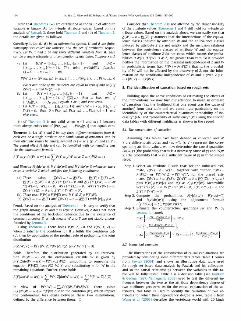

194 N. Yao, D. Miao and W. Pedrycz et al. / Expert Systems With Applications 136 (2019) 187–200

o

t

Z

l

i

b

l

b

n

i

i

m

P

5

t

o

a

i

c

d

5

Y

s

P

y

s

5

p

f

f

a

b

&

fl

t

t

t

W

Note that Theorems 1 –3 are established as the value of attribute

variable is binary. As for n -tuple attribute values, based on the

analysis of Remark 2 , there hold Theorem 2 and (ii) of Theorem 3 ,

the details are given as follows:

Corollary 1. Let (U, A ) be an information system, U and A are finite,

nonempty sets called the universe and the set of attributes, respec-

tively. Let W, Y and Z be any three different variables from A , each

can be a single attribute or a combination of attributes. Suppose x ∈ U.

(a) Let U/W = { [ x ] w 0 , . . . , [ x ] w n } (n ≥ 1) and U/Z =

{ [ x ] z 0 , . . . , [ x ] z m } (m ≥ 1) . The joint probability function

( j = 0 , . . . , n ; i = 0 , . . . , m )

P (W, Z) = { P (w 0 , z 0 ) , P (w 0 , z 1 ) , . . . , P (w j , z i ) , . . . , P (w n , z m

) }exists and none of the elements are equal to zero if and only if

Z (W ) = ∅ and W (Z) = ∅ . (b) Let U/Y = { [ x ] y 0 , . . . , [ x ] y n } (n ≥ 1) and U/Z =

{ [ x ] z 0 , . . . , [ x ] z m } (m ≥ 1) . If Y ( Z ) � = ∅ , then at least one of

{ P (z 0 | y 0 ) , . . . , P (z m

| y n ) } equals 1 or 0, and vice versa.

(c) Let U/Y = { [ x ] y 0 , . . . , [ x ] y n (n ≥ 1) } and U/Z = { [ x ] z 0 , [ x ] z 1 } . If

Y (Z) = ∅ , then 0 < P (z 0 | y 0 ) , P (z 1 | y 0 ) , . . . , P (z 1 | y n ) < 1 and

vice versa.

(i) of Theorem 3 is not valid when n ≥ 1 and m > 1 because

there always exists one of { P (z 0 | y 0 ) , . . . , P (z m

| y n ) } that equals zero.

Theorem 4. Let W, Y and Z be any three different attributes from A ,

each can be a single attribute or a combination of attributes, and let

their attribute values be binary, denoted as { w, w

′ }, { y, y ′ } and { z, z ′ } .The causal effect P ( y | do ( w )) can be identified with confounding bias

via the adjustment formula

P (Y = y | do(W = w )) =

∑

z

P (Y = y | W = w, Z = z) P (Z = z)

and likewise P ( y | do ( w

′ )), P ( y ′ | do ( w )) and P ( y ′ | do ( w

′ )) whenever there

exists a variable Z which satisfies the following conditions:

(a) There exists “Z (W ) = ∅ = W (Z) , W (Y ) ∩ Y (Z) = ∅ ,W (Y ) ∩ Y (W ) = ∅ , Z (Y ) ∩ Y (Z) = ∅ and Z (Y ) ∩ Y (W ) = ∅ ” or

“Z ( W ) � = ∅ , W (Z) = ∅ , W (Y ) ∩ Y (Z) = ∅ , W (Y ) ∩ Y (W ) = ∅ ,Z (Y ) ∩ Y (Z) = ∅ and Z (Y ) ∩ Y (W ) = ∅ ”;

(b) There exist P ( W ) � = P ( W | Z ) and P ( Y | W, Z ) � = P ( Y | W ) ;

(c) Z (W ) = ∅ = W (Z) and Z (W Y ) = ∅ = W Y (Z) with [ x ] wy � = ∅ . Proof. Based on the analysis of Theorem 1 , it is easy to verify that

the graph among Z, W and Y is acyclic. However, Z does not meet

the conditions of the back-door criterion due to the existence of

common ancestor Z , which means W and Y are not stably uncon-

founded by Lemma 3 .

Using Theorem 2 , there holds P ( W, Z ) > 0 and P ( W, Y, Z ) > 0

when Z satisfies the condition (c). If Z fulfils the conditions (a)-

(c), then by application of the product rule of probability, the joint

distribution

P (Z, W, Y ) = P (Y | W, Z) P (W | Z) P (Z)(P (Z, W, Y ) > 0)

holds. Therefore, the distribution generated by an interven-

tion do(W = w ) on the endogenous variable W is given by

P (Y, Z| do(W = w )) = P (Y | w, Z) P (Z) , amounting to removing the

equation P ( W | Z ) from P ( Z, W, Y ) and substituting w for W in the

remaining equations. Further, there holds

P (Y | do(W = w )) =

∑

Z

P (Y, Z| do(W = w )) =

∑

Z

P (Y | w, Z) P (Z) .

In view of P (Y | W ) =

∑

Z P (Y | W, Z) P (Z| W ) , there exists

P (Y | do(W = w )) � = P (Y | w ) due to the condition (b’), which implies

the confounding bias exists between these two distributions,

defined by the difference between them. �

Consider that Theorem 2 is not affected by the dimensionality

f the attribute values. Theorems 1 and 4 still hold for n -tuple at-

ribute values. Based on the analysis above, we can easily see that

(W ) = ∅ = W (Z) guarantees that the intersections of the equiva-

ence classes induced by attribute W and the equivalence classes

nduced by attribute Z are not empty and the inclusion relations

etween the equivalence classes of attribute W and the equiva-

ence classes of attribute Z do not exist, which means the proba-

ilities P ( W | Z ), P ( Z | W ), P ( W, Z ) are greater than zero. So it provides

either the information on the marginal independence of Z and W

n probabilistic terms (i.e., P (W ) = P (W | Z) ), that is, the probabil-

ty of W will not be affected by the discovery of Z , nor the infor-

ation on the conditional independence of W and Y given Z (i.e.,

(Y | W, Z) = P (Y | W ) ).

. The identification of causation based on rough sets

Building upon the above conditions of estimating the effects of

he interventions, we now turn our attention to make an estimate

f causation (i.e., the likelihood that one event was the cause of

nother) from data table and we concentrate particularly on the

dentifiability of the counterfactual quantities “probability of ne-

essity” ( PN ) and “probability of sufficiency” ( PS ) using the specific

ata tables with different highlights as shown in the sequel.

.1. The construction of causation

Assuming data tables have been defined or collected and W,

are different attributes and { w, w

′ }, { y, y ′ } represent the corre-

ponding attribute values, we now determine the causal quantities

N ( w, y ) (the probability that w is a necessary cause of y ) and PS ( w,

) (the probability that w is a sufficient cause of y ) in three simple

teps:

Step 1. Select an attribute Z such that: for the unbiased esti-

mate, Z (W ) = ∅ = W (Z) , together with “either P (W ) =P (W | Z) or P (Y | W, Z) = P (Y | W ) ”; for the biased esti-

mate, Z (W ) = ∅ = W (Z) , Z (W Y ) = ∅ = W Y (Z) , [ x ] wy � = ∅plus P ( W ) � = P ( W | Z ) and P ( Y | W, Z ) � = P ( Y | W ). Meanwhile,

W (Y ) ∩ Y (Z) = ∅ , W (Y ) ∩ Y (W ) = ∅ , Z (Y ) ∩ Y (Z) = ∅ and

Z (Y ) ∩ Y (W ) = ∅ . Step 2. Compute the probabilities P ( y | do ( w )), P ( y | do ( w

′ ))and P ( y ′ | do ( w

′ )) using the adjustment formula

P (y | do(w )

)=

∑

z P (y | w, z) P (z) .

Step 3. Estimate the counterfactual quantities PN and PS by

Lemma 4 , namely

max

{

0 , P (y ) −P (y | do(w

′ )) P(w,y )

}

≤ P N ≤

min

{

1 , P(y ′ | do(w

′ )) −P(w

′ ,y ′ ) P(w,y )

}

,

max

{

0 , P(y | do(w )) −P(y ) P(w

′ ,y ′ )

}

≤ P S ≤ min

{

1 , P(y | do(w )) −P(w,y ) P(w

′ ,y ′ )

}

.

.2. Numerical examples

The illustrations of the construction of causal explanations are

rovided by considering some different data tables. Table 1 comes

rom Pawlak (2004) and shows an illustrative data table used

or rough set based data analysis by Pawlak and his colleagues,

nd so the causal relationships between the variables in this ta-

le will be fully tested. Table 2 is a decision table (see Düntsch

Gediga, 1997; Yamaguchi, 2009 ) used to test the different in-

uences between the two as the attribute dependency degree of

wo attributes gets zero. As for the causal explanation of the at-

ributes, this table is used to identify the causation of two at-

ributes for which their dependency degree is zero. Table 3 from

ang et al. (2003) describes the vertebrate world with 20 kinds

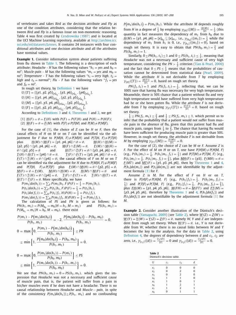
N. Yao, D. Miao and W. Pedrycz et al. / Expert Systems With Applications 136 (2019) 187–200 195

o

o

t

T

t

u

d

h

E

f

a

n

n

h

a

c

j

p

{

∅

T

F

c

a

M

F

H

P

P

0

0

W

p

o

h

c

o

P

f

q

H

d

r

P

H

t

a

s

W

γ

1

M

h

h

a

s

i

c

m

h

H

M

F

(

P

F

P

m

t

p

{

P

M

E

s

W

d

a

b

D

z

Table 2

Düntsch’s decision table.

U c 1 c 2 d

x 1 0 0 0

x 2 0 2 0

x 3 0 2 0

x 4 1 1 0

x 5 1 0 1

x 6 1 2 1

x 7 1 2 1

x 8 0 1 1

f vertebrates and takes Bird as the decision attribute and Fly as

ne of the condition attributes, considering that the relation be-

ween Bird and Fly is a famous issue on non-monotonic reasoning.

able 4 was first created by Cendrowska (1987) and is located at

he UCI Machine Learning repository, available at http://archive.ics.

ci.edu/ml/datasets/Lenses . It contains 24 instances with four con-

itional attributes and one decision attribute and all the attributes

ave nominal values.

xample 1. Consider information system about patients suffering

rom flu shown in Table 1 . The following is a description of each

ttribute: Headache - H has the following values “h 1 = yes and h 0 =o”; Muscle-pain - M has the following values “m 1 = yes and m 0 =o”; Temperature - T has the following values “t 1 = v ery high, t 2 =igh and t 3 = normal”; Flu - F has the following values “ f 1 = yes

nd f 0 = no”.

In rough set theory, by Definition 1 we have

U/ { T } = {{ p1 , p2 , p5 } [ x ] t 2 , { p3 , p6 } [ x ] t 1 , { p4 } [ x ] t 3 } , U/ { H} = {{ p1 , p4 , p6 } [ x ] h 0 , { p2 , p3 , p5 } [ x ] h 1 } , U/ { M} = {{ p1 , p3 , p4 , p6 } [ x ] m 1 , { p2 , p5 } [ x ] m 0 } , U/ { F } = {{ p1 , p2 , p3 , p6 } [ x ] f 1 , { p4 , p5 } [ x ] f 0 } . According to Definitions 3 and 4, Theorems 1 and 2 , we get

(1) H (F ) = ∅ = F (H) with P (F ) = P (F | H) and P (H) = P (H| F ) ; (2) M (F ) = ∅ = F (M) with P ( F ) � = P ( F | M ) and P ( M ) � = P ( M | F ).

For the case of (1), the choice of Z can be H or F , then the

ausal effects of H on M or on T can be identified via the ad-

ustment for F due to P ( M | H, F ) � = P ( M | H ) and P ( T | H, F ) � = P ( T | H )

lus H (M) ∩ M (F ) = { p1 , p4 , p6 } ∩ ∅ = ∅ , M (H) ∩ H (M) = p2 , p5 } ∩ { p1 , p4 , p6 } = ∅ , M (F ) ∩ F (M) = ∅ , F (M) ∩ M (H) = ∩ { p2 , p5 } = ∅ and H (T ) ∩ T (F ) = ∅ ∩ { p3 , p4 , p6 } = ∅ , (H) ∩ H (T ) = { p4 } ∩ ∅ = ∅ , T (F ) ∩ F (T ) = { p3 , p4 , p6 } ∩ ∅ = ∅ , (T ) ∩ T (H) = ∅ ∩ { p4 } = ∅ ; the causal effects of F on M or on T

an be identified via the adjustment for H due to P ( M | H, F ) � = P ( M | F )

nd P ( T | H, F ) � = P ( T | F ) plus F (M) ∩ M (H) = ∅ ∩ { p2 , p5 } = ∅ , (F ) = ∅ = F (M) , M (H) ∩ H (M) = ∅ , H (M) ∩ M (F ) = ∅ and

(T ) ∩ T (H) = ∅ ∩ { p4 } = ∅ , T (F ) ∩ F (T ) = ∅ , T (H) ∩ H (T ) = ∅ , (T ) ∩ T (F ) = ∅ . More specifically, we have

P (m 1 | do(h 1 )) =

∑

F P (m 1 | h 1 , F ) P (F ) =

1 3 = P (m 1 | h 1 ) ,

P (t 1 | do(h 1 )) =

∑

F P (t 1 | h 1 , F ) P (F ) =

1 3 = P (t 1 | h 1 ) ,

P (t 1 | do( f 1 )) =

∑

H P (t 1 | f 1 , H) P (H) =

1 2 = P (t 1 | f 1 ) ,

P (m 1 | do( f 1 )) =

∑

H P (m 1 | f 1 , H) P (H) =

3 4 = P (m 1 | f 1 ) .

The calculation of PS and PN is given as follows: for

N(h 1 , m 1 ) = P (M h 0 = m 0 | H = h 1 , M = m 1 ) and P S(h 1 , m 1 ) =

(M h 1 = m 1 | H = h 0 , M = m 0 ) , there exist

P (m 1 ) − P (m 1 | do(h 0 )

)P (h 1 , m 1 )

= −2 , P (m 0 | do(h 0 )

)− P (h 0 , m 0 )

P (h 1 , m 1 ) = 0 ,

= max

{

0 , P (m 1 ) − P

(m 1 | do(h 0 )

)P (h 1 , m 1 )

}

≤ P N

≤ min

{

1 , P (m 0 | do(h 0 )

)− P (h 0 , m 0 )

P (h 1 , m 1 )

}

= 0 ,

= max

{

0 , P (m 1 | do(h 1 )) − P (m 1 )

P (h 0 , m 0 )

}

≤ P S

≤ min

{

1 , P (m 1 | do(h 1 )) − P (h 1 , m 1 )

P (h 0 , m 0 )

}

= 0 .

e see that P N(h 1 , m 1 ) = 0 = P S(h 1 , m 1 ) , which gives the im-

ression that Headache was not a necessary and sufficient cause

f muscle pain, that is, the patient will suffer from a pain in

is/her muscles even if he does not have a headache. There is no

ausal relationship between Headache and Muscle − pain, in spite

f the consistency P ( m | do ( h )) ≥ P ( h , m ) and no confounding

1 1 1 1

(m 1 | do(h 1 )

)= P (m 1 | h 1 ) . While the attribute M depends roughly

rom H in a degree of 1 2 by employing γ{ H} ({ M} ) =

| H (M) | | U| =

1 2 (this

uantity in fact measures the dependency of m 1 from h 0 due to

(M) = { p1 , p4 , p6 } = [ x ] h 0 � [ x ] m 1 , i.e., γ{ h 0 } ({ m 1 } ) =

1 2 while the

ependency of m 1 from h 1 is 0, i.e., γ{ h 1 } ({ m 1 } ) = 0 ), based on

ough set theory. It is easy to obtain that P N(h 0 , m 1 ) =

2 3 and

S(h 0 , m 1 ) = 1 .

Similarly, 0 ≤ PN ( h 1 , t 1 ) ≤ 1 and 0 ≤ P S(h 1 , t 1 ) ≤ 1 2 , meaning that

eadache was not a necessary and sufficient cause of very high

emperature, considering the P N >

1 2 criterion ( Tian & Pearl, 20 0 0 )

nd the fact that 0 ≤ P S ≤ 1 2 means that the probabilities of cau-

ation cannot be determined from statistical data ( Pearl, 2009 ).

hile the attribute H is not derivable from T by employing

{ H} ({ T } ) =

| H (T ) | | U| = 0 , based on rough set theory.

P N( f 1 , t 1 ) = 1 and P S( f 1 , t 1 ) =

1 2 , reflecting that, we can be

00% sure that having flu was necessary for very high temperature.

eanwhile, there is 50% chance that a patient without flu and very

igh temperature would have suffered from very high temperature

ad he or she been gotten flu. While the attribute F is not deriv-

ble from T by employing γ{ F } ({ T } ) =

| F (T ) | | U| = 0 , based on rough

et theory. 1 3 ≤ P N( f 1 , m 1 ) ≤ 2

3 and

1 2 ≤ P S( f 1 , m 1 ) ≤ 1 , which permit us to

nfer that the probability that a patient would not suffer from mus-

le pain in the absence of flu, given that this patient had flu and

uscle pain, ranges from

1 3 to 2

3 . The chance that having flu would

ave been sufficient for producing muscle pain is greater than 50%.

owever, in rough set theory, the attribute F is not derivable from

by employing γ{ F } ({ M} ) =

| F (M) | | U| = 0 .

For the case of (2), the choice of Z can be M or F . Assume Z is

. For the effect of M on H or on T , one have P ( H | M ) � = P ( H | M, F )

e.g., P (h 1 | m 1 ) =

1 4 , P (h 1 | m 1 , f 1 ) =

1 3 ) and P ( T | M ) � = P ( T | M, F ) (e.g.,

(t 1 | m 1 ) =

1 2 , P (t 1 | m 1 , f 1 ) =

2 3 ), plus MH (F ) = { p3 } , F (MH) = ∅ =

(M T ) and M T (F ) = { p1 , p3 , p4 , p6 } , then by Theorems 1 and 4 ,

( h 1 | do ( m 1 )) and P ( t 1 | do ( m 1 )) are not identifiable by the adjust-

ent formula (1) for F .

Assume Z is M . For the effect of F on H or on T ,

here is P ( H | F ) � = P ( H | M, F ) (e.g., P (h 1 | f 1 ) =

1 2 , P (h 1 | m 1 , f 1 ) =

1 3 ) and P ( T | F ) � = P ( T | M, F ) (e.g., P (t 1 | f 1 ) =

1 2 , P (t 1 | m 1 , f 1 ) =

2 3 ),

lus F H (M) = { p1 , p4 , p5 , p6 } , M (F H) = ∅ = M (F T ) and F T (M) = p3 , p4 , p5 , p6 } , therefore by Theorems 1 and 4 , P ( h 1 | do ( f 1 )) and

( t 1 | do ( f 1 )) are not identifiable by the adjustment formula (1) for

.

xample 2. Consider another illustration of the Düntsch’s deci-

ion table ( Yamaguchi, 2009 ) (see Table 2 ), where W (Z) = Z (W ) = (Y ) = Y (W ) = Y (Z) = Z (Y ) = ∅ , namely W, Y and Z are indepen-

ent from rough set theory. When W (Y ) = ∅ , i.e., Y is not deriv-

ble from W , whether there is no causal links between W and Y

ecomes the key to the analysis. For the data in Table 2 , using

efinition 4 , the degrees of dependency between d and c 1 , c 2 are

ero, i.e., γ{ c 1 } ({ d} ) =

| c 1 (d) | | U| = 0 and γ{ c 2 } ({ d} ) =

| c 2 (d) | | U| = 0 .

196 N. Yao, D. Miao and W. Pedrycz et al. / Expert Systems With Applications 136 (2019) 187–200

Table 3

An information system of the vertebrate world.

U Gregarious (G) Fly (F) Egg (E) Lung (L) Bird (B) Animal name

1 no yes yes yes yes Vulture, Pheasant

2 yes yes yes yes yes Egret, Latham, Scoter

Shelduck, Sparrow

3 yes no yes yes yes Penguin, Ostrich

4 no no no yes no Opossum, Mink

5 no no yes yes no Toad, Platypus,Viper, Turtle

6 no no yes no no Dogfish

7 yes no no yes no Reindeer, Seal

8 yes no yes no no Hairtail

9 yes yes no yes no Fruit bat

i

t

s

6

d

(

t

t

t

c

t

E

t

(

g

t

a

i

a

b

t

{

{

B

To start with, based on rough set theory we have

U/ { d} = {{ x 1 , x 2 , x 3 , x 4 } [ x ] d=0 , { x 5 , x 6 , x 7 , x 8 } [ x ] d=1

} , U/ { c 1 } = {{ x 1 , x 2 , x 3 , x 8 } [ x ] c 1 =0

, { x 4 , x 5 , x 6 , x 7 } [ x ] c 1 =1 } ,

U/ { c 2 } = {{ x 1 , x 5 } [ x ] c 2 =0 , { x 2 , x 3 , x 6 , x 7 } [ x ] c 2 =2

, { x 4 , x 8 } [ x ] c 2 =1 } ,

d (c 1 ) = ∅ = d (c 2 ) , c 1 (d) = ∅ = c 2 (d) , c 1 (c 2 ) = ∅ = c 2 (c 1 ) , to-

gether with P (c 1 ) = P (c 1 | c 2 ) , P (c 2 ) = P (c 2 | c 1 ) , but P ( d | c 1 ) � = P ( d | c 1 ,

c 2 ) (e.g., P (d = 1 | c 1 = 1) =

3 4 , P (d = 1 | c 1 = 1 , c 2 = 1) = 0 ),

P ( d | c 2 ) � = P ( d | c 2 , c 1 ) (e.g., P (d = 1 | c 2 = 1) =

1 2 , P (d = 1 | c 2 = 1 , c 1 =

1) = 0 ). Therefore one can compute the effect of c 1 on d by the

adjustment for c 2 and the effect of c 2 on d by the adjustment for

c 1 . More specifically,

P (d = 1 | do(c 1 = 1)) =

∑

c 2 P (d = 1 | c 1 = 1 , c 2 ) P (c 2 ) =

3 4 = P (d =

1 | c 1 = 1) ,

P (d = 1 | do(c 1 = 0)) =

∑

c 2 P (d = 1 | c 1 = 0 , c 2 ) P (c 2 ) =

1 4 = P (d =

1 | c 1 = 0) ,

P (d = 0 | do(c 1 = 0)) =

∑

c 2 P (d = 0 | c 1 = 0 , c 2 ) P (c 2 ) =

3 4 = P (d =

0 | c 1 = 0) ,

P (d = 0 | do(c 1 = 1)) =

∑

c 2 P (d = 0 | c 1 = 1 , c 2 ) P (c 2 ) =

1 4 = P (d =

0 | c 1 = 1) ,

P (d = 0 | do(c 2 = 0)) =

∑

c 1 P (d = 0 | c 2 = 0 , c 1 ) P (c 1 ) =

1 2 = P (d =

0 | c 2 = 0) ,

P (d = 1 | do(c 2 = 0)) =

∑

c 1 P (d = 1 | c 2 = 0 , c 1 ) P (c 1 ) =

1 2 = P (d =

1 | c 2 = 0) ,

P (d = 0 | do(c 2 = 1)) =

∑

c 1 P (d = 0 | c 2 = 1 , c 1 ) P (c 1 ) =

1 2 = P (d =

0 | c 2 = 1) ,

P (d = 1 | do(c 2 = 1)) =

∑

c 1 P (d = 1 | c 2 = 1 , c 1 ) P (c 1 ) =

1 2 = P (d =

1 | c 2 = 1) ,

P (d = 0 | do(c 2 = 2)) =

∑

c 1 P (d = 0 | c 2 = 2 , c 1 ) P (c 1 ) =

1 2 = P (d =

0 | c 2 = 2) ,

P (d = 1 | do(c 2 = 2)) =

∑

c 1 P (d = 1 | c 2 = 2 , c 1 ) P (c 1 ) =

1 2 = P (d =

1 | c 2 = 2) .

By employing Lemma 4 , there exist 2 3 ≤ P N(c 1 = 1 , d = 1) ≤ 1 , 2

3 ≤ P S(c 1 = 1 , d = 1) ≤ 1 , 0 ≤P N(c 1 = 0 , d = 1) ≤ 1 and 0 ≤ P S(c 1 = 0 , d = 1) ≤ 1 ; 2

3 ≤ P N(c 1 =0 , d = 0) ≤ 1 , 2

3 ≤ P S(c 1 = 0 , d = 0) ≤ 1 , 0 ≤ P N(c 1 = 1 , d = 0) ≤ 1

and 0 ≤ P S(c 1 = 1 , d = 0) ≤ 1 ;

0 ≤ P N(c 2 = 0 , d = 0) ≤ 1 , 0 ≤ P S(c 2 = 0 , d = 0) ≤ 1 3 , 0 ≤

P N(c 2 = 1 , d = 0) ≤ 1 , 0 ≤ P S(c 2 = 1 , d = 0) ≤ 1 3 , 0 ≤ P N(c 2 =

2 , d = 0) ≤ 1 and 0 ≤ P S(c 2 = 2 , d = 0) ≤ 1 3 ;

0 ≤ P N(c 2 = 0 , d = 1) ≤ 1 , 0 ≤ P S(c 2 = 0 , d = 1) ≤ 1 3 , 0 ≤

P N(c 2 = 1 , d = 1) ≤ 1 , 0 ≤ P S(c 2 = 1 , d = 1) ≤ 1 3 , 0 ≤ P N(c 2 =

2 , d = 1) ≤ 1 and 0 ≤ P S(c 2 = 2 , d = 1) ≤ 1 3 .

It is easy to find that the above causal explanation of c 1 , c 2 and

d provides a more specific and more convincing argument than the

attribute dependency degrees of the three γ{ c 1 } ({ d} ) = 0 . 5625 and

γ{ c 2 } ({ d} ) = 0 . 3958 from Yamaguchi (2009) (different from the de-

pendency in Definition 4 ). We see that the probability that d = 1

would not have occurred in the absence of c 1 = 1 given that c 1 = 1

and d = 1 did in fact occur is greater than

2 3 , in other words, there

is at least 67% chance that c 1 = 1 was necessary for the production

of d = 1 . The probability that setting c 1 = 1 would produce d = 1

n a situation where d � = 1 and c 1 � = 1 in fact occur is also greater

han

2 3 , meaning that there is at least 67% chance that c 1 = 1 was

ufficient for the production of d = 1 . Similarly, there is at least

7% chance that c 1 = 0 was necessary and sufficient for the pro-

uction of d = 0 . Note that under the condition of no-confounding

P (y | do(x )) = P (y | x ) ) the lower bound for PN often needs to meet

he P N >

1 2 criterion ( Tian & Pearl, 20 0 0 ), and 0 ≤ P S ≤ 1

2 means

hat the probabilities of causation cannot be determined from sta-

istical data ( Pearl, 2009 ). Accordingly, the causal relation between

2 and d as well as c 1 = 0 ( c 1 = 1 ) and d = 1 ( d = 0 ) cannot be de-

ermined from Table 2 .

xample 3. Take another classic example of information sys-

em on vertebrates with 20 different animals from Wang et al.

2003) shown in Table 3 , where Bird is the decision attribute, { Gre-

arious, Fly, Egg, Lung } are the condition attributes.

Referring to Table 3 , let F = f 1 and F = f 0 represent, respec-

ively, it can fly and cannot fly, B = b 1 and B = b 0 represent it is

bird and not a bird, G = g 1 and G = g 0 represent it is gregar-

ous and not gregarious, E = e 1 and E = e 0 represent laying eggs

nd not laying eggs and L = l 1 and L = l 0 represent using lung for

reathing and not using lung for breathing. Based on rough set

heory, it is obvious that:

U/ { Bird} = {{ 1 , 2 , 3 } [ x ] b 1 , { 4 , 5 , 6 , 7 , 8 , 9 } [ x ] b 0 } , U/ { F ly } = {{ 1 , 2 , 9 } [ x ] f 1 , { 3 , 4 , 5 , 6 , 7 , 8 } [ x ] f 0 } , U/ { Egg} = {{ 1 , 2 , 3 , 5 , 6 , 8 } [ x ] e 1 , { 4 , 7 , 9 } [ x ] e 0 } , U/ { Lung} = {{ 1 , 2 , 3 , 4 , 5 , 7 , 9 } [ x ] l 1 , { 6 , 8 } [ x ] l 0 } , U/ { Gregarious } = {{ 1 , 4 , 5 , 6 } [ x ] g 0 , { 2 , 3 , 7 , 8 , 9 } [ x ] g 1 } , U/ { Egg, Lung} = {{ 1 , 2 , 3 , 5 } [ x ] e 1 ,l 1 , { 6 , 8 } [ x ] e 1 ,l 0 , { 4 , 7 , 9 } [ x ] e 0 ,l 1 } , U/ { Gregarious, Egg} = {{ 2 , 3 , 8 } [ x ] e 1 ,g 1 , { 4 } [ x ] e 0 ,g 0 , { 1 , 5 , 6 } [ x ] e 1 ,g 0 ,

7 , 9 } [ x ] e 0 ,g 1 } , U/ { Gregarious, Lung} = {{ 2 , 3 , 7 , 9 } [ x ] l 1 ,g 1 , { 1 , 4 , 5 } [ x ] l 1 ,g 0 , { 6 } [ x ] l 0 ,g 0 ,

8 } [ x ] l 0 ,g 1 } , U/ { Gregarious, Lung, Egg} = {{ 1 , 5 } [ x ] l 1 ,e 1 ,g 0 , { 2 , 3 } [ x ] l 1 ,e 1 ,g 1 , { 4 } [ x ] l 1 ,e 0 ,g 0 , { 6 } [ x ] l 0 ,e 1 ,g 0 , { 7 , 9 } [ x ] l 1 ,e 0 ,g 1 , { 8 } [ x ] l 0 ,e 1 ,g 1 } . y Theorems 1 and 2 , we obtain

(1) F ly (Gregarious ) = ∅ = Gregarious (F ly ) with P ( F ) � = P ( F | G ) (e.g.,

P ( f 1 ) =

8 20 , P ( f 1 | g 1 ) =

6 11 ) and P ( G ) � = P ( G | F ) (e.g., P (g 1 ) =

11 20 ,

P (g 1 | f 1 ) =

6 8 ), P ( B | F ) � = P ( B | F, G ) and P ( B | G ) � = P ( B | G, F ) (e.g.,

P (b 1 | f 1 ) =

7 8 , P (b 1 | f 1 , g 1 ) =

5 6 , P (b 1 | g 1 ) =

7 11 );

(2) F ly (Egg) = ∅ = Egg (F ly ) with P ( F ) � = P ( F | E ) (e.g., P ( f 1 | e 1 ) =7

15 ) and P ( E ) � = P ( E | F ) (e.g., P (e 1 ) =

15 20 , P (e 1 | f 1 ) =

7 8 ),

P ( B | F ) � = P ( B | F, E ) and P ( B | E ) � = P ( B | E, F ) (e.g., P (b 1 | f 1 , e 1 ) = 1 ,

P (b 1 | e 1 ) =

9 15 );

(3) F ly (Bird) = ∅ = Bird (F ly ) with P ( F ) � = P ( F | B ) (e.g., P ( f 1 | b 1 ) =7 9 ) and P ( B ) � = P ( B | F ) (e.g., P (b 1 ) =

9 20 , P (b 1 | f 1 ) =

7 8 ), P ( G | B,

F ) � = P ( G | B ) � = P ( G | F ) (e.g., P (g 1 | b 1 , f 1 ) =

5 7 , P (g 1 | f 1 ) =

6 11 ,

P (g 1 | b 1 ) =

7 ), P ( E | B, F ) � = P ( E | B ) � = P ( E | F ) (e.g., P (e 1 | f 1 , b 0 ) = 0 ,

9

N. Yao, D. Miao and W. Pedrycz et al. / Expert Systems With Applications 136 (2019) 187–200 197

t

c

P

P

∅

E

F

o

f ∑P

f ∑P

i

F

a

i

c

l

d

i

a

o

B

m

a

E

U

a

2

∅

P

P

e

γ

P

p

1

P

1

1

a

P

P

a

b

a

P (e 1 | f 1 ) =

7 8 , P (e 1 | b 0 ) =

6 11 ), P ( L | B, F ) � = P ( L | B ) � = P ( L | F ) (e.g.,

P (l 1 | f 0 , b 0 ) =

4 5 , P (l 1 | f 0 ) =

5 6 , P (l 1 | b 0 ) =

9 11 );

(4) Gregarious (Bird) = ∅ = Bird (Gregarious ) with P ( G ) � = P ( G | B )

(e.g., P (g 1 ) =

11 20 , P (g 1 | b 1 ) =

7 9 ) and P ( B ) � = P ( B | G ) (e.g.,

P (b 1 ) =

9 20 , P (b 1 | g 1 ) =

7 11 ), P ( F | B ) � = P ( F | B, G ) and

P ( F | G ) � = P ( F | G, B ) (e.g., P ( f 1 | b 1 ) =

7 9 , P ( f 1 | b 1 , g 1 ) =

5 7 ,

P ( f 1 | g 1 ) =

6 11 ), P ( E | B, G ) � = P ( E | B ) � = P ( E | G ) (e.g., P (e 1 | b 0 ) =

6 11 ,

P (e 1 | g 1 ) =

8 11 , P (e 1 | b 0 , g 1 ) =

1 4 ), P ( L | B, G ) � = P ( L | B ) � = P ( L | G )

(e.g., P (l 1 | b 0 ) =

9 11 , P (l 1 | g 1 ) =

10 11 , P (l 1 | b 0 , g 1 ) =

3 4 ).

(5) Egg (Gregarious ) = ∅ = Gregarious (Egg) , P ( G ) � = P ( G | E ), P ( B | G,

E ) � = P ( B | G ), P ( B | G, E ) � = P ( B | E ) (e.g., P (b 1 | g 1 ) =

7 11 , P (b 1 | e 1 ) =

9 15 , P (b 1 | g 1 , e 1 ) =

7 8 );

(6) Lung (Gregarious ) = ∅ = Gregarious (Lung) , P ( G ) � = P ( G | L ), P ( B | G,

L ) � = P ( B | G ), P ( B | G, L ) � = P ( B | L ) (e.g., P (b 1 | g 1 ) =

7 11 , P (b 1 | l 1 ) =

7 18 , P (b 1 | g 1 , l 1 ) =

7 10 ).

Further, according to Theorem 4 , we conclude that

1. the effect P ( b | do ( f )) is not identifiable by the adjustment for-

mula for Gregarious in view of F ly, Bird (Gregarious ) = { 3 , 9 }and Gregarious (F ly, Bird) = ∅ .

2. the effect P ( b | do ( f )) is not identifiable by the adjust-

ment formula for Egg due to F ly, Bird (Egg) = { 1 , 2 , 3 , 9 } and

Egg (F ly, Bird) = ∅ . 3. the effects P ( g | do ( f )), P ( e | do ( f )) and P ( l | do ( f ))

are not identifiable by the adjustment formula

for Bird due to F ly, Gregarious (Bird) = { 1 , 4 , 5 , 6 } ,F ly, Egg (Bird) = { 1 , 2 , 4 , 7 , 9 } , F ly, Lung (Bird) = { 6 , 8 } and

Bird (F ly, Gregarious ) = ∅ = Bird (F ly, Egg) = Bird (F ly, Lung) ;

the effects P ( b | do ( g )), P ( g | do ( b )), P ( b | do ( e )), P ( e | do ( b )) and

P ( l | do ( b )) are not identifiable by the adjustment for-

mula for Fly due to Bird, Gregarious (F ly ) = { 1 , 4 , 5 , 6 } ,Bird, Egg (F ly ) = { 5 , 6 , 8 } , Bird, Lung (F ly ) = { 6 , 8 } and

F ly (Bird, Gregarious ) = ∅ = F ly (Bird, Egg) = F ly (Bird, Lung) .

4. the effects P ( f | do ( g )), P ( e | do ( g )) and P ( l | do ( g )) are

not identifiable by the adjustment formula for

Bird because of Gregarious, F ly (Bird) = { 1 , 4 , 5 , 6 } ,Gregarious, Egg (Bird) = { 4 , 7 , 9 } , Gregarious, Lung (Bird) ={ 6 , 8 } and Bird (Gregarious, F ly ) = ∅ = Bird (Gregarious, Egg) =Bird (Gregarious, Lung) ;

P ( f | do ( b )) is not identifiable by the adjustment for-

mula for Gregarious Bird, F ly (Gregarious ) = { 3 , 9 } and

Gregarious (Bird, F ly ) = ∅ ; P ( e | do ( b )), P ( b | do ( e )), P ( b | do ( l )) and P ( l | do ( b )) are not

identifiable via the adjustment formula for Gregari-

ous with confounding bias due to [ x ] b 1 ,e 0 = ∅ = [ x ] b 1 ,l 0 (which implies P (b 1 , e 0 , g) = 0 = P (b 1 , l 0 , g) ) in spite

of Gregarious (Bird, Egg) = ∅ = Bird, Egg (Gregarious ) and

Gregarious (Bird, Lung) = ∅ = Bird, Lung (Gregarious ) .

5. the effect P ( b | do ( g )) is not identifiable by the adjustment

formula for Egg and Lung due to Bird, Gregarious (Egg) ={ 1 , 2 , 3 } = Bird, Gregarious (Lung) , Egg (Bird, Gregarious ) = ∅ =Lung (Bird, Gregarious ) .

To put it another way, when omitting the number of

he animals in the column of “Animal name” and re-

alculating the probabilities, we have P (F ) = P (F | E) but

( B | F, E ) � = P ( B | F ) � = P ( B | E ) (e.g., P (b 1 | f 1 , e 1 ) = 1 , P (b 1 | f 1 ) =

2 3 ,

(b 1 | e 1 ) =

1 2 ), F ly (Bird) ∩ Bird (Egg) = ∅ ∩ { 1 , 2 , 3 } = ∅ , F ly (Bird) =

= Bird (F ly ) , Egg (Bird) ∩ Bird (Egg) = { 4 , 7 , 9 } ∩ { 1 , 2 , 3 } = ∅ ,gg (Bird) ∩ Bird (F ly ) = { 4 , 7 , 9 } ∩ ∅ = ∅ , Egg (Bird) ∩ Bird (Egg) = ∅ , ly (Bird) ∩ Bird (F ly ) = ∅ , and further, using Theorems 1 and 2 ,

ne can calculate the causal effect of Fly on Bird without con-

ounding bias via the adjustment for Egg , namely P (b 1 | do( f 1 )) =

E P (b 1 | f 1 , E ) P (E ) = P (b 1 | f 1 , e 1 ) P (e 1 ) + P (b 1 | f 1 , e 0 ) P (e 0 ) =

2 3 =

(b | f ) and the causal effect of Egg on Bird without con-

1 1

ounding bias via the adjustment for Fly , i.e., P (b 1 | do(e 1 )) =

F P (b 1 | e 1 , F ) P (F ) = P (b 1 | e 1 , f 1 ) P ( f 1 ) + P (b 1 | e 1 , f 0 ) P ( f 0 ) =

1 2 =

(b 1 | e 1 ) . Accordingly, one get 3 4 ≤ P N( f 1 , b 1 ) = P (B f 0 = b 0 | F = f 1 , B = b 1 ) ≤ 1 , 3 5 ≤ P S( f 1 , b 1 ) = P (B f 1 = b 1 | F = f 0 , B = b 0 ) ≤ 4

5 ,

P N(e 1 , b 1 ) = P (B e 0 = b 0 | E = e 1 , B = b 1 ) = 1 ,

P S(e 1 , b 1 ) = P (B e 1 = b 1 | E = e 0 , B = b 0 ) =

1 2 ,

P N(e 0 , b 0 ) = P (B e 1 = b 1 | E = e 0 , B = b 0 ) =

1 2 ,

P S(e 0 , b 0 ) = P (B e 0 = b 0 | E = e 1 , B = b 1 ) = 1 .

Further the degree of dependency between Bird and Fly

s zero, i.e., γ{ F ly } ({ Bird} ) =

| F ly (Bird) | | U| = 0 = γ{ Bird} ({ F ly } ) due to

ly (Bird) = ∅ = Bird (F ly ) . The degree of dependency between Bird

nd Egg is k = γ{ Egg} ({ Bird} ) =

| Egg (Bird) | | U| =

1 3 , i.e., k = γe 1 (b 1 ) =

| e 1 (b 1 ) | = | [ x ] e 1 ⊆[ x ] b 1 |

| U| = 0 , k = γe 0 (b 0 ) =

| e 0 (b 0 ) | = | [ x ] e 0 ⊆[ x ] b 0 |

| U| =

1 3 .

Using the proposed results to the data in Table 3 , we get the

nterventional interpretation and counterfactual analysis for the

onditional attributes Fly and Egg and the decision attribute Bird ,

earning more information than that conveyed by attribute depen-

ency. Additionally we find from Table 3 that the column of “An-

mal name” has no effect on the lower approximation but can

ffect statistical independence. This might relate to the presence

f the possible sample selection bias ( Bareinboim & Pearl, 2016;

areinboim & Tian, 2015 ) and the results given by omitting “Ani-

al name” column may be viewed as a reference in data analysis

nd inference.

xample 4. Take another dataset for fitting contact lenses from the

CI Machine Learning repository. The detailed description of each

ttribute is as follows (see Table 4 ):

Age of the patient -a : it has the following values: (1) young, (2)

pre-presbyopic, (3) presbyopic.

Spectacle prescription -b : it has the following values: (1) myope,

(2) hypermetrope.

Astigmatic -c : it has the following values: (1) no, (2) yes.

Tear production rate -d : it has the following values: (1) reduced,

(2) normal.

Decision -e : it is a decision attribute that contains the following

values: (1) hard contact lenses, (2) soft contact lenses, (3) no

contact lenses.

According to Definitions 3 and 4, Theorems 1 and

, it is easily obtained that a (b) = ∅ = b (a ) , a (c) = = c (a ) , a (d) = ∅ = d (a ) , P (a ) = P (a | b) , P (a ) = P (a | c) , (a ) = P (a | d) , P ( e | ab ) � = P ( e | a ) � = P ( e | b ), P ( e | ac ) � = P ( e | a ) � = P ( e | c ),

( e | ad ) � = P ( e | a ) � = P ( e | d ), a (e ) = ∅ = e (a ) , e (b) = ∅ = b (e ) , c (e ) = ∅ , ( c ) � = ∅ , d (e ) = ∅ , e ( d ) � = ∅ , γ{ a } ({ e } ) = 0 = γ{ b} ({ e } ) = γ{ c} ({ e } ) ={ d} ({ e } ) . Further we get the unbiased estimate of P ( e | do ( a )),

( e | do ( b )), P ( e | do ( c )) and P ( e | do ( d )). By Definition 10 and Lemma 4 ,

lus P N >

1 2 and P S >

1 2 , it is concluded that

P N(a = 1 , e = 1) ∈ [ 1 2 , 1] , P S(a = 1 , e = 1) ∈ [ 1 7 , 2 7 ] ; P N(b =

, e = 1) ∈ [ 2 3 , 1] , P S(b = 1 , e = 1) ∈ [ 2 11 , 3 11 ] ;

P N(c = 2 , e = 1) = 1 , P S(c = 2 , e = 1) =

1 3 , P N(c = 1 , e = 2) = 1 ,

S(c = 1 , e = 2) =

5 12 ;

P N(d = 2 , e = 1) = 1 , P S(d = 2 , e = 1) =

1 3 , P N(d = 2 , e = 2) =

, P S(d = 2 , e = 2) =

5 12 , P N(d = 1 , e = 3) =

3 4 , P S(d = 1 , e = 3) =

.

For the combination of attributes, it is easily found that

b (c) = ∅ = c (ab) , ab (d) = ∅ = d (ab) , abc (d) = ∅ = d (abc) ,

(ab) = P (ab| c) = P (ab| d) , P (abc) = P (abc| d) , P ( e | ab, c ) � = P ( e | ab ),

( e | ab, d ) � = P ( e | ab ), P ( e | abc, d ) � = P ( e | abc ), ab (e ) = ∅ = e (ab) ,

bc ( e ) � = ∅ , e (abc) = ∅ , abc (e ) ∩ e (d) = ∅ , d (e ) = ∅ = e (abc) ,

c (a ) = ∅ = a (bc) , bc (e ) = ∅ = e (bc) , P (bc) = P (bc| a ) , P ( e | bc,

) � = P ( e | bc ), bcd (a ) = ∅ = a (bcd) , bcd ( e ) � = ∅ , e (bcd) = ∅ ,

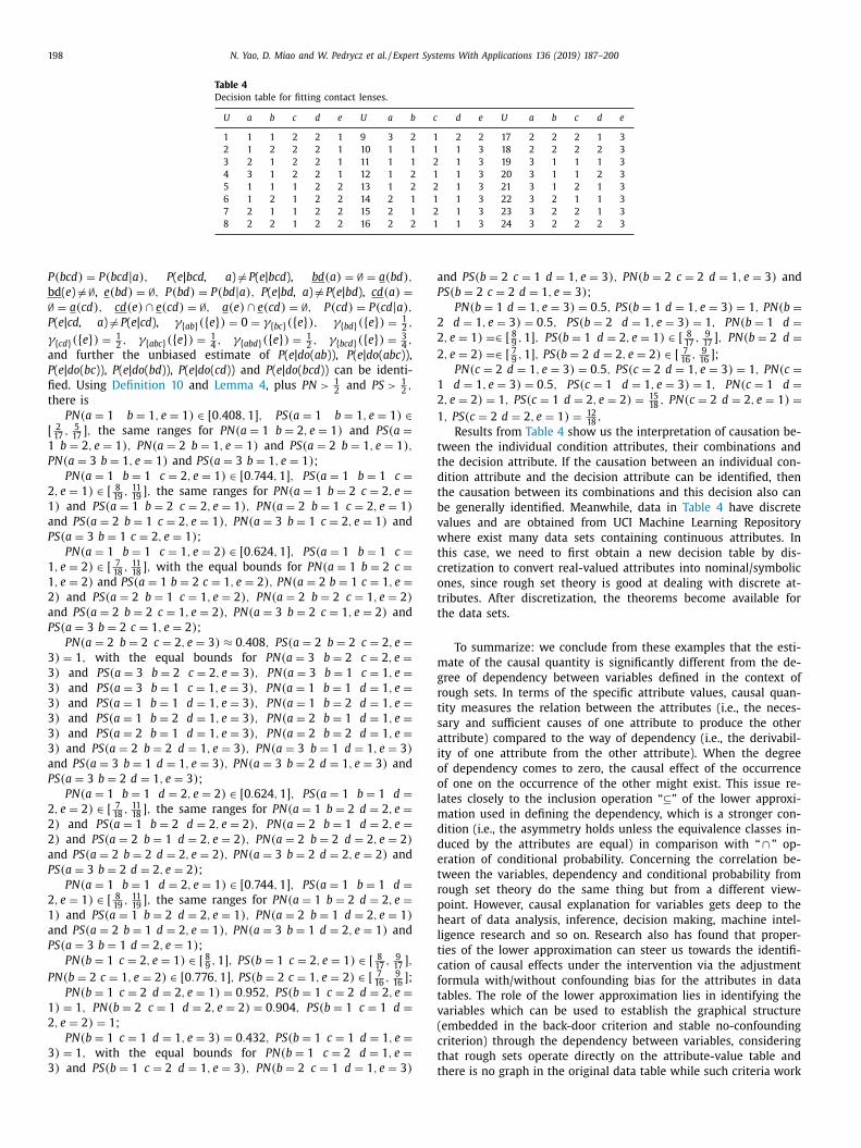
198 N. Yao, D. Miao and W. Pedrycz et al. / Expert Systems With Applications 136 (2019) 187–200

Table 4

Decision table for fitting contact lenses.

U a b c d e U a b c d e U a b c d e

1 1 1 2 2 1 9 3 2 1 2 2 17 2 2 2 1 3

2 1 2 2 2 1 10 1 1 1 1 3 18 2 2 2 2 3

3 2 1 2 2 1 11 1 1 2 1 3 19 3 1 1 1 3

4 3 1 2 2 1 12 1 2 1 1 3 20 3 1 1 2 3

5 1 1 1 2 2 13 1 2 2 1 3 21 3 1 2 1 3

6 1 2 1 2 2 14 2 1 1 1 3 22 3 2 1 1 3

7 2 1 1 2 2 15 2 1 2 1 3 23 3 2 2 1 3

8 2 2 1 2 2 16 2 2 1 1 3 24 3 2 2 2 3

a

P

2

2

2

1

2

1

t

t

d

t

b

v

w

t

c

o

t

t

m

g

r

t

s

a

i

o

o

l

m

d

d

e

t

r

p

h

l

t

c

f

t

v

(

c

t

P (bcd) = P (bcd| a ) , P ( e | bcd, a ) � = P ( e | bcd ), bd (a ) = ∅ = a (bd) ,

bd ( e ) � = ∅ , e (bd) = ∅ , P (bd) = P (bd| a ) , P ( e | bd, a ) � = P ( e | bd ), cd (a ) =∅ = a (cd) , cd (e ) ∩ e (cd) = ∅ , a (e ) ∩ e (cd) = ∅ , P (cd) = P (cd| a ) ,P ( e | cd, a ) � = P ( e | cd ), γ{ ab} ({ e } ) = 0 = γ{ bc} ({ e } ) , γ{ bd} ({ e } ) =

1 2 ,

γ{ cd} ({ e } ) =

1 2 , γ{ abc} ({ e } ) =

1 4 , γ{ abd} ({ e } ) =

1 2 , γ{ bcd} ({ e } ) =

3 4 ,

and further the unbiased estimate of P ( e | do ( ab )), P ( e | do ( abc )),

P ( e | do ( bc )), P ( e | do ( bd )), P ( e | do ( cd )) and P ( e | do ( bcd )) can be identi-

fied. Using Definition 10 and Lemma 4 , plus P N >

1 2 and P S >

1 2 ,

there is

P N(a = 1 b = 1 , e = 1) ∈ [0 . 408 , 1] , P S(a = 1 b = 1 , e = 1) ∈[ 2 17 ,

5 17 ] , the same ranges for P N(a = 1 b = 2 , e = 1) and P S(a =

1 b = 2 , e = 1) , P N(a = 2 b = 1 , e = 1) and P S(a = 2 b = 1 , e = 1) ,

P N(a = 3 b = 1 , e = 1) and P S(a = 3 b = 1 , e = 1) ;

P N(a = 1 b = 1 c = 2 , e = 1) ∈ [0 . 744 , 1] , P S(a = 1 b = 1 c =2 , e = 1) ∈ [ 8

19 , 11 19 ] , the same ranges for P N(a = 1 b = 2 c = 2 , e =

1) and P S(a = 1 b = 2 c = 2 , e = 1) , P N(a = 2 b = 1 c = 2 , e = 1)

and P S(a = 2 b = 1 c = 2 , e = 1) , P N(a = 3 b = 1 c = 2 , e = 1) and

P S(a = 3 b = 1 c = 2 , e = 1) ;

P N(a = 1 b = 1 c = 1 , e = 2) ∈ [0 . 624 , 1] , P S(a = 1 b = 1 c =1 , e = 2) ∈ [ 7

18 , 11 18 ] , with the equal bounds for P N(a = 1 b = 2 c =

1 , e = 2) and P S(a = 1 b = 2 c = 1 , e = 2) , P N(a = 2 b = 1 c = 1 , e =2) and P S(a = 2 b = 1 c = 1 , e = 2) , P N(a = 2 b = 2 c = 1 , e = 2)

and P S(a = 2 b = 2 c = 1 , e = 2) , P N(a = 3 b = 2 c = 1 , e = 2) and

P S(a = 3 b = 2 c = 1 , e = 2) ;

P N(a = 2 b = 2 c = 2 , e = 3) ≈ 0 . 408 , P S(a = 2 b = 2 c = 2 , e =3) = 1 , with the equal bounds for P N(a = 3 b = 2 c = 2 , e =3) and P S(a = 3 b = 2 c = 2 , e = 3) , P N(a = 3 b = 1 c = 1 , e =3) and P S(a = 3 b = 1 c = 1 , e = 3) , P N(a = 1 b = 1 d = 1 , e =3) and P S(a = 1 b = 1 d = 1 , e = 3) , P N(a = 1 b = 2 d = 1 , e =3) and P S(a = 1 b = 2 d = 1 , e = 3) , P N(a = 2 b = 1 d = 1 , e =3) and P S(a = 2 b = 1 d = 1 , e = 3) , P N(a = 2 b = 2 d = 1 , e =3) and P S(a = 2 b = 2 d = 1 , e = 3) , P N(a = 3 b = 1 d = 1 , e = 3)

and P S(a = 3 b = 1 d = 1 , e = 3) , P N(a = 3 b = 2 d = 1 , e = 3) and

P S(a = 3 b = 2 d = 1 , e = 3) ;

P N(a = 1 b = 1 d = 2 , e = 2) ∈ [0 . 624 , 1] , P S(a = 1 b = 1 d =2 , e = 2) ∈ [ 7

18 , 11 18 ] , the same ranges for P N(a = 1 b = 2 d = 2 , e =

2) and P S(a = 1 b = 2 d = 2 , e = 2) , P N(a = 2 b = 1 d = 2 , e =2) and P S(a = 2 b = 1 d = 2 , e = 2) , P N(a = 2 b = 2 d = 2 , e = 2)

and P S(a = 2 b = 2 d = 2 , e = 2) , P N(a = 3 b = 2 d = 2 , e = 2) and

P S(a = 3 b = 2 d = 2 , e = 2) ;

P N(a = 1 b = 1 d = 2 , e = 1) ∈ [0 . 744 , 1] , P S(a = 1 b = 1 d =2 , e = 1) ∈ [ 8

19 , 11 19 ] , the same ranges for P N(a = 1 b = 2 d = 2 , e =

1) and P S(a = 1 b = 2 d = 2 , e = 1) , P N(a = 2 b = 1 d = 2 , e = 1)

and P S(a = 2 b = 1 d = 2 , e = 1) , P N(a = 3 b = 1 d = 2 , e = 1) and

P S(a = 3 b = 1 d = 2 , e = 1) ;

P N(b = 1 c = 2 , e = 1) ∈ [ 8 9 , 1] , P S(b = 1 c = 2 , e = 1) ∈ [ 8 17 , 9 17 ] ,

P N(b = 2 c = 1 , e = 2) ∈ [0 . 776 , 1] , P S(b = 2 c = 1 , e = 2) ∈ [ 7 16 ,

9 16 ] ;

P N(b = 1 c = 2 d = 2 , e = 1) = 0 . 952 , P S(b = 1 c = 2 d = 2 , e =1) = 1 , P N(b = 2 c = 1 d = 2 , e = 2) = 0 . 904 , P S(b = 1 c = 1 d =2 , e = 2) = 1 ;

P N(b = 1 c = 1 d = 1 , e = 3) = 0 . 432 , P S(b = 1 c = 1 d = 1 , e =3) = 1 , with the equal bounds for P N(b = 1 c = 2 d = 1 , e =3) and P S(b = 1 c = 2 d = 1 , e = 3) , P N(b = 2 c = 1 d = 1 , e = 3)

t

nd P S(b = 2 c = 1 d = 1 , e = 3) , P N(b = 2 c = 2 d = 1 , e = 3) and

S(b = 2 c = 2 d = 1 , e = 3) ;

P N(b = 1 d = 1 , e = 3) = 0 . 5 , P S(b = 1 d = 1 , e = 3) = 1 , P N(b = d = 1 , e = 3) = 0 . 5 , P S(b = 2 d = 1 , e = 3) = 1 , P N(b = 1 d = , e = 1) = ∈ [ 8 9 , 1] , P S(b = 1 d = 2 , e = 1) ∈ [ 8 17 ,

9 17 ] , P N(b = 2 d =

, e = 2) = ∈ [ 7 9 , 1] , P S(b = 2 d = 2 , e = 2) ∈ [ 7 16 ,

9 16 ] ;

P N(c = 2 d = 1 , e = 3) = 0 . 5 , P S(c = 2 d = 1 , e = 3) = 1 , P N(c = d = 1 , e = 3) = 0 . 5 , P S(c = 1 d = 1 , e = 3) = 1 , P N(c = 1 d = , e = 2) = 1 , P S(c = 1 d = 2 , e = 2) =

15 18 , P N(c = 2 d = 2 , e = 1) =

, P S(c = 2 d = 2 , e = 1) =

12 18 .

Results from Table 4 show us the interpretation of causation be-

ween the individual condition attributes, their combinations and

he decision attribute. If the causation between an individual con-

ition attribute and the decision attribute can be identified, then

he causation between its combinations and this decision also can

e generally identified. Meanwhile, data in Table 4 have discrete

alues and are obtained from UCI Machine Learning Repository

here exist many data sets containing continuous attributes. In

his case, we need to first obtain a new decision table by dis-

retization to convert real-valued attributes into nominal/symbolic

nes, since rough set theory is good at dealing with discrete at-

ributes. After discretization, the theorems become available for

he data sets.

To summarize: we conclude from these examples that the esti-

ate of the causal quantity is significantly different from the de-

ree of dependency between variables defined in the context of

ough sets. In terms of the specific attribute values, causal quan-

ity measures the relation between the attributes (i.e., the neces-

ary and sufficient causes of one attribute to produce the other

ttribute) compared to the way of dependency (i.e., the derivabil-

ty of one attribute from the other attribute). When the degree

f dependency comes to zero, the causal effect of the occurrence

f one on the occurrence of the other might exist. This issue re-

ates closely to the inclusion operation “⊆” of the lower approxi-

ation used in defining the dependency, which is a stronger con-

ition (i.e., the asymmetry holds unless the equivalence classes in-

uced by the attributes are equal) in comparison with “ ∩ ” op-

ration of conditional probability. Concerning the correlation be-

ween the variables, dependency and conditional probability from

ough set theory do the same thing but from a different view-

oint. However, causal explanation for variables gets deep to the

eart of data analysis, inference, decision making, machine intel-

igence research and so on. Research also has found that proper-

ies of the lower approximation can steer us towards the identifi-

ation of causal effects under the intervention via the adjustment

ormula with/without confounding bias for the attributes in data

ables. The role of the lower approximation lies in identifying the

ariables which can be used to establish the graphical structure

embedded in the back-door criterion and stable no-confounding

riterion) through the dependency between variables, considering

hat rough sets operate directly on the attribute-value table and

here is no graph in the original data table while such criteria work

N. Yao, D. Miao and W. Pedrycz et al. / Expert Systems With Applications 136 (2019) 187–200 199

s

n

p

c

c

a

p

b

s

t

d

w

M

s

p

t

e

d

a

6

i

n

n

c

t

v

b

m

i

b

m

e

l

w

p

w

d

w

h

a

a

o

c

c

r

(

l

t

i

A

o

o

i

c

i

u

g

r

g

t

t

i

a

c

t

i

i

a

k

t

t

t

l

f

c

l

D

c

i

C

a

e

i

P

v

i

-

A

e

t

t

N

N

6

M

R

B

B

B

B

B

C

C

C

C

D

traight on the (directed) acyclic graph. As the examples exhibited,

ot all the causation of attributes can be estimated using the pro-

osed results. This depends mainly on the dissatisfaction with the

onditions for the use of the adjustment formula when setting the

ovariates (having the potential for adjustment) as a single vari-

ble. How to tackle this issue requires further effort s, f or exam-

le, study the situation where graph structures embedded in the

ack-door criterion with the covariates (a subset of which can be

elected for adjustment) viewed as a set of attribute variables in

he rough set framework by referring to the work on Pearl’s back-

oor criterion ( Maathuis & Colombo, 2015; Pearl, 2009 ) and the

ork on the graphs involved in this criterion ( Enright, Madden, &

adden, 2013; Ramasso & Denoeux, 2014 ) or develop the repre-

entation of the notions of intervention and counterfactual in the

ure rough set terminology by drawing inspiration possibly from

he “do ” operator and its generalizations ( Benferhat, 2010; Boukhris

t al., 2013; Pearl, 2009 ) along with the application of rough sets to

irected graphs ( Chiaselotti, Ciucci, Gentile, & Infusino, 2017; Chi-

selotti, Gentile, & Infusino, 2018 ).

. Conclusions

The causal explanations behind data play an important role

n problem solving, everyday reasoning, judgment, and commu-

ication about the world. Pearl’s profound insight of the combi-

ation of graphical models and probability achieves mathematical

omputation of causality. Following this idea, we provide condi-

ions for estimating cause–effect relationships from an attribute-

alue information system with complete data and discrete values

y fusing the lower approximation of the set into the mathematical

odel of causality. Theorem 1 presents the conditions of uncover-

ng causal effects under the intervention with no-confounding bias

y the adjustment formula, which extends the back-door adjust-

ent with a single covariate from rough sets’ angle. It is strength-

ned by Theorems 2 and 3 , verifying that the combination of the

ower approximation and the probability can be used to decide

hat measurements are needed for identifiability. Theorem 4 de-

icts the conditions of the effect estimate under the intervention

ith confounding bias by the adjustment formula. Since rough sets

o not use any parameters outside data and do reason starting

ith the primitive data, the method developed in this paper can

elp to understand and manipulate the identification of causation

bout attribute-value tables. Also this is a simple attempt to an-

lyze causality in rough set theory by applying causal quantities

f causal inference, which expands the applicability of structural

ausal models, and paves the way for portraying interventions and

ounterfactuals in rough set terms, which enriches the content of

ough set theory.

Causality is shown in Lake, Ullman, Tenenbaum, and Gershman

2017) as one of the core ingredients for building AI (artificial intel-

igence) systems with more human-like learning and thought, and

he machine learning systems in Pearl (2019) that can reason about

nterventions and counterfactuals can serve as the basis for strong

I. We close this section by presenting some speculative thoughts

n the future research. An interesting topic is to apply the results

f identifying causation between attributes in the process of learn-

ng from examples, i.e., learning characteristic features of each con-

ept from features of all given instances of the concept and deriv-

ng decision rules from the given examples. The issue of powerful

nderstanding for AI systems, such as understanding scenes and

enerating natural language captions, is a promising research di-

ection that might be solved by employing the proposed results to

lue the objects and their use together or to relate the actions with

he goals and intentions. Another topic is to use the proposed tools

o creativity action and concept approximation, such as construct-

ng new concepts by gluing some existing concepts with coherence

nd purpose. It is also promising to infuse the proposed tools for

ausality within the rough set framework into the intelligent sys-

ems based on granular computing ( Pedrycz, 2013 ) and the exist-

ng machine learning models. When the attribute-value data table

s given with missing data, the discovering of causality between

ttributes is a challenging work, along with finding how lack of

nowledge would affect the systems’ ability to learn. Another wor-

hy directions include the impact of newly observed instances on

he already acquired causal knowledge, the possible integration of

he proposed results of causation into emotional research for intel-

igent machines, the measure of the complexity of time and space

or the proposed tools when the number of attributes within in-

omplete/complete data table becomes very large, and other re-

ated issues to AI system research.

eclaration of Competing Interest

The authors declare that they have no known competing finan-

ial interests or personal relationships that could have appeared to

nfluence the work reported in this paper.

redit authorship contribution statement

Ning Yao: Conceptualization, Methodology, Validation, Formal

nalysis, Data curation, Writing - original draft, Writing - review &

diting. Duoqian Miao: Conceptualization, Formal analysis, Writ-

ng - review & editing, Supervision, Funding acquisition. Witold

edrycz: Methodology, Formal analysis, Supervision, Writing - re-

iew & editing, Validation. Hongyun Zhang: Formal analysis, Writ-

ng - review & editing, Funding acquisition. Zhifei Zhang: Writing

review & editing, Data curation, Investigation.

cknowledgments

We are very grateful to the editors and two anonymous review-

rs for their incisive comments and for providing insightful and ex-

remely helpful suggestions on the early version of this manuscript

o improve our work. This research was supported in parts by the

ational Key R&D Program of China (grant number 213); National

atural Science Foundation of China (grant numbers 61673301 ,

1573255 , 61573259 , 61673299 , 61603278 ); and Major Project of

inistry of Public Security (grant number 20170 0 04 ).

eferences

areinboim, E. , & Pearl, J. (2016). Causal inference and the data-fusion problem. Pro-

ceedings of the National Academy of Sciences, 113 (27), 7345–7352 . areinboim, E. , & Tian, J. (2015). Recovering causal effects from selection bias. In

Proceedings of the 29th AAAI conference on artificial intelligence (pp. 3475–3481).AAAI Press .

enferhat, S. (2010). Interventions and belief change in possibilistic graphical mod-

els. Artificial Intelligence, 174 (2), 177–189. doi: 10.1016/j.artint.2009.11.012 . enferhat, S. , & Smaoui, S. (2007). Possibilistic causal networks for handling inter-

ventions: a new propagation algorithm. In Proceedings of the 22nd national con-ference on artificial intelligence (pp. 373–378). AAAI Press .

oukhris, I., Elouedi, Z., & Benferhat, S. (2013). Dealing with external actions in be-lief causal networks. International Journal of Approximate Reasoning, 54 (8), 978–

999. doi: 10.1016/j.ijar.2013.02.009 .

endrowska, J. (1987). PRISM: An algorithm for inducing modular rules. In-ternational Journal of Man-Machine Studies, 27 (4), 349–370. doi: 10.1016/

S0020-7373(87)80003-2 . hiaselotti, G., Ciucci, D., Gentile, T., & Infusino, F. (2017). Rough set theory and

digraphs. Fundamenta Informaticae, 153 (4), 291–325. doi: 10.3233/FI- 2017- 1542 . hiaselotti, G., Gentile, T., & Infusino, F. (2018). Granular computing on informa-

tion tables: Families of subsets and operators. Information Sciences, 442 , 72–102.doi: 10.1016/j.ins.2018.02.046 .

iucci, D., Chiaselotti, G., Gentile, T., & Infusino, F. (2016). Generalizations of rough

set tools inspired by graph theory. Fundamenta Informaticae, 148 (1–2), 207–227.doi: 10.3233/FI- 2016- 1431 .

üntsch, I., & Gediga, G. (1997). Statistical evaluation of rough set dependency anal-ysis. International Journal of Human-Computer Studies, 46 (5), 589–604. doi: 10.

1006/ijhc.1996.0105 .

200 N. Yao, D. Miao and W. Pedrycz et al. / Expert Systems With Applications 136 (2019) 187–200

R

T

T

W

W

W

Y

Y

Y

Y

Z

Z

Z

Z

Z

Düntsch, I., & Gediga, G. (2001). Roughian: Rough information analysis. InternationalJournal of Intelligent Systems, 16 (1), 121–147. doi: 10.1002/1098-111X(200101)16:

13.0.CO;2-Z . Enright, C. G., Madden, M. G., & Madden, N. (2013). Bayesian networks for mathe-

matical models: Techniques for automatic construction and efficient inference.International Journal of Approximate Reasoning, 54 (2), 323–342. doi: 10.1016/j.ijar.

2012.10.004 . Lake, B., Ullman, T., Tenenbaum, J., & Gershman, S. (2017). Building machines that

learn and think like people. Behavioral and Brain Sciences, 40 , e253. doi: 10.1017/

S0140525X16001837 . Lingras, P., & Haider, F. (2015). Partially ordered rough ensemble clustering

for multigranular representations. Intelligent Data Analysis, 19 (s1), S103–S116.doi: 10.3233/IDA-150772 .

Maathuis, M. H., & Colombo, D. (2015). A generalized back-door criterion. The Annalsof Statistics, 43 (3), 1060–1088. doi: 10.1214/14-AOS1295 .

Neyman, J. (1923). On the application of probability theory to agricultural experi-

ments. Essay on principles. Section 9. Translated and edited by D.M. Da browskaand T.P. Speed from the Polish original (1990). Statistical Science, 5 (4), 465–

472 . Pawlak, Z. (1991). Rough sets: Theoretical aspects of reasoning about data . Kluwer Aca-

demic Publishers . Pawlak, Z. (2004). Some issues on rough sets. In J. F. Peters, A. Skowron, J. W. Grzy-

mała-Busse, B. Kostek, R. W. Swiniarski, & M. S. Szczuka (Eds.), Transactions on

rough sets i (pp. 1–58). Springer Berlin Heidelberg . Pawlak, Z., & Skowron, A. (2007). Rudiments of rough sets. Information Sciences,

177 (1), 3–27. doi: 10.1016/j.ins.2006.06.003 . Pearl, J. (2009). Causality: Models, reasoning, and inference (2nd ed.). Cambridge Uni-

versity Press . Pearl, J. (2010). The foundations of causal inference. Sociological Methodology, 40 (1),

75–149 .

Pearl, J. (2015). Causal thinking in the twilight zone. Observational Studies, 1 ,200–204 .

Pearl, J. (2019). The seven tools of causal inference, with reflections on machinelearning. Communications of the ACM, 62 , 54–60 .

Pedrycz, W. (2013). Granular computing : Analysis and design of intelligent systems .CRC Press .

Peters, J. F. , & Skowron, A. (2006). Some contributions by Zdzisław Pawlak. In

G.-Y. Wang, J. F. Peters, A. Skowron, & Y. Yao (Eds.), Rough sets and knowledgetechnology (pp. 1–11). Springer Berlin Heidelberg .

Qian, J., Miao, D., Zhang, Z., & Yue, X. (2014). Parallel attribute reduction algorithmsusing mapreduce. Information Sciences, 279 , 671–690. doi: 10.1016/j.ins.2014.04.

019 . Ramasso, E., & Denoeux, T. (2014). Making use of partial knowledge about hidden

states in hmms: An approach based on belief functions. IEEE Transactions on

Fuzzy Systems, 22 (2), 395–405. doi: 10.1109/TFUZZ.2013.2259496 .

aza, M. S., & Qamar, U. (2018). A heuristic based dependency calculation techniquefor rough set theory. Pattern Recognition, 81 , 309–325. doi: 10.1016/j.patcog.2018.

04.009 . Rubin, D. B. (1974). Estimating causal effects of treatments in randomized and non-

randomized studies. Journal of Educational Psychology, 66 (5), 688–701 . Spirtes, P. , Glymour, C. , & Scheines, R. (1993). Causation, prediction, and search .

Springer New York . ian, J. , & Pearl, J. (20 0 0). Probabilities of causation: Bounds and identification. An-

nals of Mathematics and Artificial Intelligence, 28 (1–4), 287–313 .

ran, A. D., Arch-Int, S., & Arch-Int, N. (2018). A rough set approach for approxi-mating differential dependencies. Expert Systems with Applications, 114 , 488–502.

doi: 10.1016/j.eswa.2018.06.025 . ang, J. , Zhao, M. , Zhao, K. , & Han, S. (2003). Multilevel data summarization from

information systems: A “rule + exception” approach. AI Communications, 16 (1),17–39 .

right, S. (1921). Correlation and causation. Journal of Agricultural Research, 20 ,

557–585 . u, W. Z., Qian, Y., Li, T. J., & Gu, S. M. (2017). On rule acquisition in incomplete

multi-scale decision tables. Information Sciences, 378 , 282–302. doi: 10.1016/j.ins.2016.03.041 .

amaguchi, D. (2009). Attribute dependency functions considering data efficiency.International Journal of Approximate Reasoning, 51 (1), 89–98. doi: 10.1016/j.ijar.

20 09.08.0 02 .

ao, J., & Azam, N. (2015). Web-based medical decision support systems for three-way medical decision making with game-theoretic rough sets. IEEE Transactions

on Fuzzy Systems, 23 , 3–15. doi: 10.1109/TFUZZ.2014.2360548 . ao, N. , Miao, D. , Zhang, Z. , & Lang, G. (2016). Probabilistic estimation for gen-

eralized rough modus ponens and rough modus tollens. In V. Flores, F. Go-mide, A. Janusz, C. Meneses, D. Miao, G. Peters, . . . Y. Yao (Eds.), Rough sets

(pp. 166–176). Springer International Publishing .

ao, Y. (2011). The superiority of three-way decisions in probabilistic rough setmodels. Information Sciences, 181 (6), 1080–1096. doi: 10.1016/j.ins.2010.11.019 .

hang, X., & Miao, D. (2016). Quantitative/qualitative region-change uncer-tainty/certainty in attribute reduction: Comparative region-change analyses

based on granular computing. Information Sciences, 334–335 , 174–204. doi: 10.1016/j.ins.2015.11.037 .

hou, J., & Miao, D. (2011). β-Interval attribute reduction in variable precision rough

set model. Soft Computing, 15 (8), 1643–1656. doi: 10.10 07/s0 050 0- 011- 0693- 4 . iarko, W. (1993). Variable precision rough set model. Journal of Computer and Sys-

tem Science, 46 (1), 39–59. doi: 10.1016/0 022-0 0 0 0(93)90 048-2 . iarko, W. (2007). Dependencies in structures of decision tables. In M. Kryszkiewicz,

J. F. Peters, H. Rybinski, & A. Skowron (Eds.), Rough sets and intelligent systemsparadigms (pp. 113–121). Springer Berlin Heidelberg .

iarko, W. (2008). Probabilistic approach to rough sets. International Journal of Ap-

proximate Reasoning, 49 (2), 272–284. doi: 10.1016/j.ijar.2007.06.014 .