expert systems with applications - فرداپیپر to 0/1 knapsack problem for detection of the...
TRANSCRIPT
Expert Systems with Applications 41 (2014) 3712–3725
Contents lists available at ScienceDirect
Expert Systems with Applications
journal homepage: www.elsevier .com/locate /eswa
An improved firefly algorithm for solving dynamic multidimensionalknapsack problems
0957-4174/$ - see front matter � 2013 Elsevier Ltd. All rights reserved.http://dx.doi.org/10.1016/j.eswa.2013.11.040
⇑ Corresponding author. Tel.: +90 232 3017600.E-mail address: [email protected] (A. Baykasoglu).
Adil Baykasoglu ⇑, Fehmi Burcin OzsoydanDokuz Eylül University, Faculty of Engineering, Department of Industrial Engineering, _Izmir, Turkey
a r t i c l e i n f o a b s t r a c t
Keywords:Firefly algorithmGenetic algorithmDifferential evolutionDynamic optimizationMultidimensional knapsack problem
There is a wide range of publications reported in the literature, considering optimization problems wherethe entire problem related data remains stationary throughout optimization. However, most of the real-life problems have indeed a dynamic nature arising from the uncertainty of future events. Optimizationin dynamic environments is a relatively new and hot research area and has attracted notable attention ofthe researchers in the past decade. Firefly Algorithm (FA), Genetic Algorithm (GA) and DifferentialEvolution (DE) have been widely used for static optimization problems, but the applications of thosealgorithms in dynamic environments are relatively lacking. In the present study, an effective FA introduc-ing diversity with partial random restarts and with an adaptive move procedure is developed and pro-posed for solving dynamic multidimensional knapsack problems. To the best of our knowledge thispaper constitutes the first study on the performance of FA on a dynamic combinatorial problem. In orderto evaluate the performance of the proposed algorithm the same problem is also modeled and solved byGA, DE and original FA. Based on the computational results and convergence capabilities we concludedthat improved FA is a very powerful algorithm for solving the multidimensional knapsack problemsfor both static and dynamic environments.
� 2013 Elsevier Ltd. All rights reserved.
1. Introduction The authors used a binary encoding technique and a penalizing
The area of evolutionary computation widely focuses on staticoptimization where the entire problem related data or variables re-main stationary throughout optimization procedure. However,most of the real-life problems are dynamic in nature which meansthat a solution approach is expected to be adaptive to environmen-tal changes. Therefore, tracking moving optima or high-qualitysolutions becomes the main purpose rather than optimizing a pre-cisely predefined system. Evolutionary algorithms which havebeen widely studied for static optimization problems attractedan increasing attention over the past years on dynamic optimiza-tion problems (DOPs) (Branke, 2002; Jin & Branke, 2005; Morrison,2004; Weicker, 2003). There are reported research theses (Liekens,2005; Wilke, 1999) and edited volumes (Yang, Ong, & Jin, 2007) de-voted to this research area in its infancy.
DOPs can be divided into two major fields as combinatorial andcontinuous. Because this study focuses on the combinatorial part,continuous DOPs are outside of the scope of this paper. However, arecently published study (Brest et al., 2013) provides a comprehen-sive research for continuous part. On combinatorial DOP partRohlfshagen and Yao (2011) presented an extended work ofRohlfshagen and Yao (2008) on the dynamic subset sum problem.
procedure to avoid infeasibility. Various stationary extensions ofknapsack problems (Kellerer, Pferschy, & Pisinger, 2004) have beencommonly studied by the researches. Because the dynamic versionof multidimensional knapsack problem (dynMKP) is discussed here,related work is provided in the following.
Branke, Orbayı, and Uyar (2006) studied the effects of solutionrepresentation techniques for dynMKP. They used three types ofrepresentations which are, binary encoding, permutation encoding,and real valued encoding with weight-coding. The authors generateddynamic environments using a stationary environment as a base,and updated the changing parameters using normal distribution.A penalizing procedure is also presented in their studies in orderto handle with infeasibilities.
Karaman and Uyar (2004) introduced a novel method whichuses the environment-quality measuring technique which was ap-plied to 0/1 knapsack problem for detection of the changes in theenvironment. Afterwards, Karaman, Uyar, and Eryigit (2005) classi-fied the dynamic evolutionary algorithms into four categories andthey proposed an evolutionary algorithm considering the previousrelated work for 0/1 knapsack problem.
Kleywegt & Papastavrou, 1998, 2001 reported a stochastic/dynamic knapsack problem where items dynamically arrive withrespect to a Poisson distribution. A distinctive feature was thatthe profit and unit resource consumption values of the itemsbecome visible as they arrive. In their problem the aim was to

A. Baykasoglu, F.B. Ozsoydan / Expert Systems with Applications 41 (2014) 3712–3725 3713
maximize the profit accepting the most appropriate items, reject-ing rest of the items, where rejection causes a penalty. The sameproblem was reported by Hartman and Perry (2006). The authorsutilized linear programming and duality for a quick approximationparticularly on large scaled problems.
Karve et al. (2006) introduced and evaluated a middlewaretechnology, capable of allocating resources to web applicationsthrough dynamic application instance placement which is a relatedproblem of dynMKP. Kimbrel, Steinder, Sviridenko, and Tantawi(2005) reported a similar study.
Farina, Deb, and Amato (2004) proposed several test cases fordynamic multi-objective problems and the authors addressed thedynMKP as an appropriate problem for applications and implemen-tations. For a similar purpose, Li and Yang (2008) proposed a gener-alized dynamic environment generator which can be instantiatedinto binary, real-valued and combinatorial problem domains. As re-ported in their studies, the proposed dynamic environment gener-ator could be implemented to knapsack problems as well.
Adaptation of parameters was widely studied in the field of dy-namic evolutionary algorithms. Thierens (2002) proposed adaptivemutation rate schemes for GAs, in order to prevent non-trivialdecisions beforehand. Dean, Goemans, and Vondrák (2008) pre-sented a stochastic version of 0/1 knapsack problem where thevalue of the items are deterministic but the unit resource con-sumptions are assumed as randomly distributed.
As it can be seen from the previous studies related to the dy-namic version of knapsack problems, compared to well known sta-tic extensions, there are relatively far less reported publications.This is one of the main motivations behind the present study as dy-namic knapsack problems have many practical implications. Thesecond motivation is to investigate the performance of a relativelynew and promising optimizer FA and its improved version (as pro-posed in this paper) on this dynamic optimization problem in com-parison to very well known and widely used evolutionaryalgorithms GA and DE.
The rest of the paper is organized as follows: static and dynamicversions of MKP is presented in Section 2, solution approaches DE,GA and FA are discussed in detail in Section 3. Sections 4–5 repre-sent experimental results and conclusion, respectively.
1 http://people.brunel.ac.uk/�mastjjb/jeb/orlib/files/mknapcb4.txt.
2. Dynamic multidimensional knapsack problem
As reported in the studies of Branke et al. (2006), MKP is in theNP-complete class and according to Kellerer et al. (2004) knapsackproblems have been widely used as combinatorial benchmarkproblems of evolutionary algorithms. In addition, because MKPhas numerous dynamic real-life applications such as cargo loading,selecting project funds, budget management, cutting stock, etc.,dynamic version of MKP was used as benchmark environment inthis study. Well known stationary version of MKP was formalizedas follows in the scientific literature:
maximizeXn
j¼1
pjxj ð1Þ
s:t:Xn
j¼1
wijxj 6 ci 8i 2 I ð2Þ
xj 2 f0;1g8j 2 J ð3Þ
where J = {1, 2, 3, . . ., n} set of items, I = {1, 2, 3, . . ., m} set of dimen-sions of knapsack, n is the number of items, m is the number ofdimensions of the knapsack, xj is the binary variable denotingwhether the jth item is selected or not, pj is profit of the jth item,cj is the capacity of the ith dimension of the knapsack and wij is
the unit resource consumption of the jth item for the ith dimensionof the knapsack and all parameters are assumed to be positive.
Literature includes well known benchmark generators for DOPs(Morrison, 2004; Rohlfshagen, Lehre, & Yao, 2009; Ursem, Krink,Jensen, & Michalewicz, 2002; Yang, 2003). Those generators brieflytranslate a well-known static problem into a dynamic versionusing specialized procedures. Dynamism is adopted here as thechanges of the parameters after a predefined simulation time unitssimilar to Branke et al. (2006). Simulation time unit representsnumber of iterations allocated for each environment. In otherwords it represents a frequency of dynamic change. The less num-ber of simulation time units yields to more frequent changes andvice versa. In this study, a series of 1000 iterations is adopted asthe frequency of changes.
An initial environment is required as a basis in order to dynam-ically generate other environments. Therefore, as Branke et al.(2006), the first instance of mknapcb4.txt1 was used as the basisenvironment. This instance includes 100 items and 10 dimensionswith a tightness ratio of 0.25. After a change occurs, the parametersare updated as stated below.
pj ¼ pj � ð1þ Nð0;rpÞÞ ð4Þ
wij ¼ wij � ð1þ Nð0;rwÞÞ ð5Þ
ci ¼ ci � ð1þ Nð0;rcÞÞ ð6Þ
The standard deviation of normal distributions of each parame-ter are assumed to be equal and rp = rw = rc = 0.05 which yields toan average 11 out of the 100 items to be assigned or removed(Branke et al., 2006).
Distinctly from the other authors, neither lower nor upperbounds for those dynamic parameters are employed here. It’sthought that if a change (whether with respect to a probability dis-tribution or other sources of dynamism) occurs in dynamic envi-ronment, bounding it might not exactly reflect real-lifeapplications. Solution approaches for DE, GA and FA are discussedin the following section.
3. Solution approaches
As stated in the aforementioned sections DOPs considerably dif-fer from the traditional stationary problems (Baykasoglu &Durmus�oglu, 2011, 2013). In the typical black box optimizations,a population based algorithm starts from randomly chosen pointsin the search space or mapped representations because of the lackof information. The algorithm is expected to converge through gen-erations. Like many other factors, complexity of problem has anapparent impact on the convergence capability of the algorithm.However, assuming that the changing optimum is around the pre-vious one, intuition suggests that using the information of the pre-viously visited points might make a complex problem to be solved.In other words, once a high-quality solution is reached for a timeperiod of a DOP then the tracking good solutions might be easierunless a severe change occurs. This can also reduce the computa-tional complexity of the problem (Rohlfshagen & Yao, 2011). A ba-sic approach to solve a DOP might be restarting the algorithm withits initially set parameters once a change occurs. In other wordsDOP can be handled as a sequence of stationary problems.Conversely, the algorithm can be allowed to run in a continuousmanner and not take any action to changes. Considering thoseopposite approaches, it can be seen that, convergence which is adesirable feature for stationary environments might not be enough
3714 A. Baykasoglu, F.B. Ozsoydan / Expert Systems with Applications 41 (2014) 3712–3725
on DOPs. Diversity is required to be introduced and to be main-tained on appropriate levels through generations for DOPs.
In the literature, there are published works mainly focusing onthe adaptation of traditional evolutionary algorithms to dynamicproblems. Rossi, Barrientos, and del Cerro (2007) proposed adap-tive mutation operators for tracking of changing optima. The twowell-known techniques, hyper-mutation (Cobb, 1990) and randomimmigrants (Grefenstette, 1992) are mainly based on the adapta-tion of the population using adaptive parameters. Other recentadaptation of parameters based approaches jDE and SaDE were re-ported in the studies of Brest, Greiner, Boškovic, Mernik, andZumer (2006) and Qin, Huang, and Suganthan (2009) where scalingfactors and crossover rates were used as self-adaptive parameters.
Another widespread technique is exploiting implicit or explicitmemories, where memory is embedded in solution representation(Goldberg & Smith, 1987; Hadad & Eick, 1997) or is a record of thepreviously revealed good solutions (Yang, 2005, 2006).
Additionally, Branke, Kau, Schmidt, and Schmeck (2000) andYazdani, Nasiri, Sepas-Moghaddam, and Meybodi (2013) proposeda multi population based approach where whole population is di-vided into smaller sized populations. According to this approachwhile a subpopulation is tasked with convergence and solutionimprovements, some other subpopulations introduce and maintaindiversity.
A considerably different approach was proposed in van Hemert,van Hoyweghen, Lukschandl, and Verbeeck (2001), Bosman (2005),Bosman and Poutrè (2007). According to their approaches, the dataof the problem is collected during the optimization process and aninference is performed in order to predict the future events in aproactive manner.
In the present study an improved version of FA with an adapta-tion technique applicable on both stationary and dynamic environ-ments is proposed. However, for a fair comparison and evaluationon the base algorithms, any improving procedures such as adaptivememory, specialized crossover or mutation techniques are notallowed.
3.1. Differential evolution
DE is a population based approach which uses the differences ofthe individuals in the population and like other evolutionaryalgorithms. It was originally introduced by Storn and Price(1995). DE uses crossover mutation and selection operators. Muta-tion here is assumed as the difference of randomly chosen individ-uals. There are different schemes of DE reported in the literature
Fig. 1. A pseudo
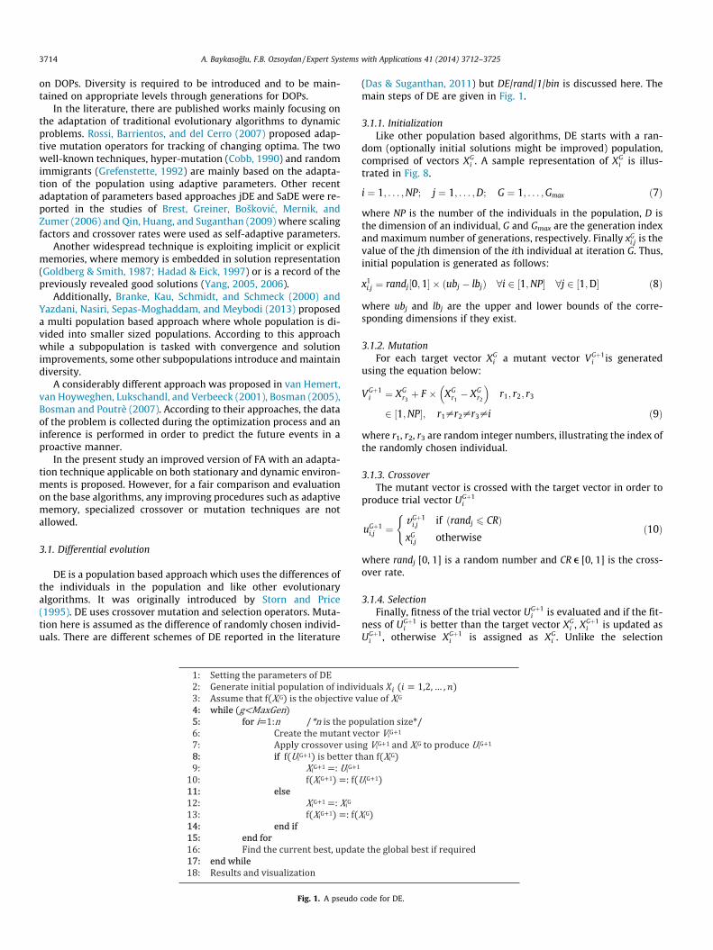
(Das & Suganthan, 2011) but DE/rand/1/bin is discussed here. Themain steps of DE are given in Fig. 1.
3.1.1. InitializationLike other population based algorithms, DE starts with a ran-
dom (optionally initial solutions might be improved) population,comprised of vectors XG
i . A sample representation of XGi is illus-
trated in Fig. 8.
i ¼ 1; . . . ;NP; j ¼ 1; . . . ;D; G ¼ 1; . . . ;Gmax ð7Þ
where NP is the number of the individuals in the population, D isthe dimension of an individual, G and Gmax are the generation indexand maximum number of generations, respectively. Finally xG
i;j is thevalue of the jth dimension of the ith individual at iteration G. Thus,initial population is generated as follows:
x1i;j ¼ randj½0;1� � ðubj � lbjÞ 8i 2 ½1;NP� 8j 2 ½1;D� ð8Þ
where ubj and lbj are the upper and lower bounds of the corre-sponding dimensions if they exist.
3.1.2. MutationFor each target vector XG
i a mutant vector VGþ1i is generated
using the equation below:
VGþ1i ¼ XG
r3þ F � XG
r1� XG
r2
� �r1; r2; r3
2 ½1;NP�; r1–r2–r3–i ð9Þ
where r1, r2, r3 are random integer numbers, illustrating the index ofthe randomly chosen individual.
3.1.3. CrossoverThe mutant vector is crossed with the target vector in order to
produce trial vector UGþ1i
uGþ1i;j ¼
vGþ1i;j if ðrandj 6 CRÞ
xGi;j otherwise
(ð10Þ
where randj [0, 1] is a random number and CR e [0, 1] is the cross-over rate.
3.1.4. SelectionFinally, fitness of the trial vector UGþ1
i is evaluated and if the fit-ness of UGþ1
i is better than the target vector XGi , XGþ1
i is updated asUGþ1
i , otherwise XGþ1i is assigned as XG
i . Unlike the selection
code for DE.
A. Baykasoglu, F.B. Ozsoydan / Expert Systems with Applications 41 (2014) 3712–3725 3715
operator as in GAs, selection here gives equal chances to all trialvectors generated from target vectors.
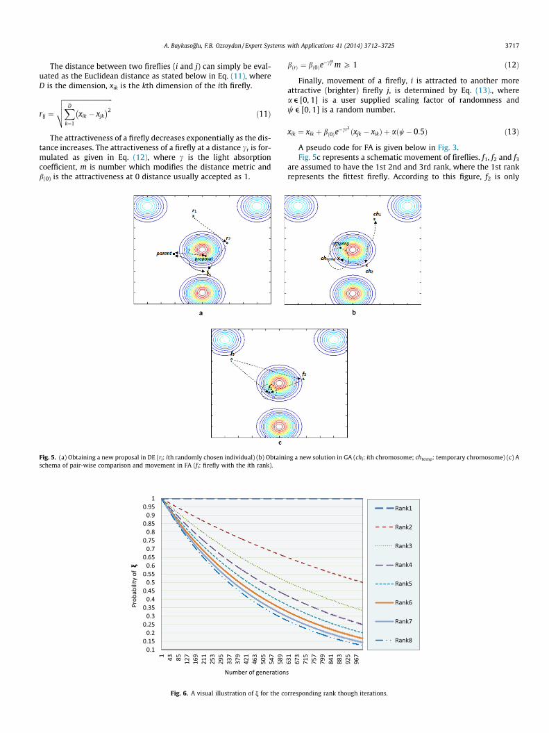
An illustration of operations in DE is given in Fig. 5a. As can beseen from the figure summation/differentiation and scaling opera-tions are applied to r1, r2 and r3. The mutant is crossed with target(parent). Finally, the trial is replaced with target if it achieves a bet-ter fitness.
Fig. 2. A pseudo
Fig. 3. A pseudo
Fig. 4. A pseudo
3.2. Genetic algorithm
GA simulates the behavior of evolution of organisms. It’s awidely used stochastic search technique which can findsolutions to various NP-hard problems (Goldberg, 1989;Holland, 1975; Lim, 2012; Thengade & Dondal, 2012). GA canalso be considered as a basis of evolutionary algorithms. A
code for GA.
code for FA.
code for FA2.
Tabl
e1
Ada
ptiv
epr
obab
iliti
esn
thro
ugh
iter
atio
ns(n
=(r
ank i
)�f ).
Iter
atio
ns
Ran
kof
fire
flie
sin
the
swar
m(1
stra
nk
isth
efi
ttes
t)
12
34
56
7���
500
501
502
503
504
505
506
���
995
996
997
998
999
1000
11,
000
1,00
01,
000
1,00
01,
000
1,00
01,
000
���
1,00
01,
000
1,00
01,
000
1,00
01,
000
1,00
0���
1,00
01,
000
1,00
01,
000
1,00
01,
000
21,
000
0,99
90,
999
0,99
80,
997
0,99
70,
996
���
0,70
80,
707
0,70
70,
706
0,70
60,
705
0,70
5���
0,50
20,
502
0,50
10,
501
0,50
10,
500
31,
000
0,99
90,
998
0,99
70,
996
0,99
50,
993
���
0,57
80,
577
0,57
70,
576
0,57
50,
575
0,57
4���
0,33
60,
335
0,33
50,
334
0,33
40,
334
41,
000
0,99
90,
997
0,99
60,
994
0,99
30,
992
���
0,50
10,
500
0,49
90,
499
0,49
80,
497
0,49
7���
0,25
20,
252
0,25
10,
251
0,25
10,
250
51,
000
0,99
80,
997
0,99
50,
994
0,99
20,
990
���
0,44
80,
447
0,44
60,
446
0,44
50,
444
0,44
4���
0,20
20,
202
0,20
10,
201
0,20
10,
200
. ... ..
. ... ..
. ... ..
. ... ..
. ... ..
. ... ..
. ... ..
. ... ..
���
. ... ..
. ... ..
. ... ..
501,
000
0,99
60,
992
0,98
80,
984
0,98
10,
977
���
0,14
20,
141
0,14
10,
140
0,14
00,
139
0,13
9���
0,02
00,
020
0,02
00,
020
0,02
00,
020
511,
000
0,99
60,
992
0,98
80,
984
0,98
10,
977
���
0,14
10,
140
0,13
90,
139
0,13
80,
138
0,13
7���
0,02
00,
020
0,02
00,
020
0,02
00,
020
521,
000
0,99
60,
992
0,98
80,
984
0,98
00,
977
���
0,13
90,
139
0,13
80,
138
0,13
70,
137
0,13
6���
0,02
00,
020
0,02
00,
019
0,01
90,
019
531,
000
0,99
60,
992
0,98
80,
984
0,98
00,
976
���
0,13
80,
137
0,13
70,
136
0,13
60,
135
0,13
5���
0,01
90,
019
0,01
90,
019
0,01
90,
019
541,
000
0,99
60,
992
0,98
80,
984
0,98
00,
976
���
0,13
70,
136
0,13
60,
135
0,13
40,
134
0,13
3���
0,01
90,
019
0,01
90,
019
0,01
90,
019
551,
000
0,99
60,
992
0,98
80,
984
0,98
00,
976
���
0,13
50,
135
0,13
40,
134
0,13
30,
133
0,13
2���
0,01
90,
019
0,01
80,
018
0,01
80,
018
. ... ..
. ... ..
. ... ..
. ... ..
. ... ..
. ... ..
. ... ..
. ... ..
���
. ... ..
. ... ..
. ... ..
951,
000
0,99
50,
991
0,98
60,
982
0,97
70,
973
���
0,10
30,
103
0,10
20,
102
0,10
10,
101
0,10
0���
0,01
10,
011
0,01
10,
011
0,01
10,
011
961,
000
0,99
50,
991
0,98
60,
982
0,97
70,
973
���
0,10
30,
102
0,10
20,
101
0,10
10,
100
0,10
0���
0,01
10,
011
0,01
10,
011
0,01
10,
010
971,
000
0,99
50,
991
0,98
60,
982
0,97
70,
973
���
0,10
20,
102
0,10
10,
101
0,10
00,
100
0,09
9���
0,01
10,
011
0,01
00,
010
0,01
00,
010
981,
000
0,99
50,
991
0,98
60,
982
0,97
70,
973
���
0,10
10,
101
0,10
10,
100
0,10
00,
099
0,09
9���
0,01
00,
010
0,01
00,
010
0,01
00,
010
991,
000
0,99
50,
991
0,98
60,
982
0,97
70,
973
���
0,10
10,
101
0,10
00,
100
0,09
90,
099
0,09
8���
0,01
00,
010
0,01
00,
010
0,01
00,
010
100
1,00
00,
995
0,99
10,
986
0,98
20,
977
0,97
3���
0,10
00,
100
0,10
00,
099
0,09
90,
098
0,09
8���
0,01
00,
010
0,01
00,
010
0,01
00,
010
Val
ues
of1
0,00
00,
001
0,00
20,
003
0,00
40,
005
0,00
6..
.���
0,49
90,
50,
501
0,50
20,
503
0,50
40,
505
���
0,99
40,
995
0,99
60,
997
0,99
80,
999
3716 A. Baykasoglu, F.B. Ozsoydan / Expert Systems with Applications 41 (2014) 3712–3725
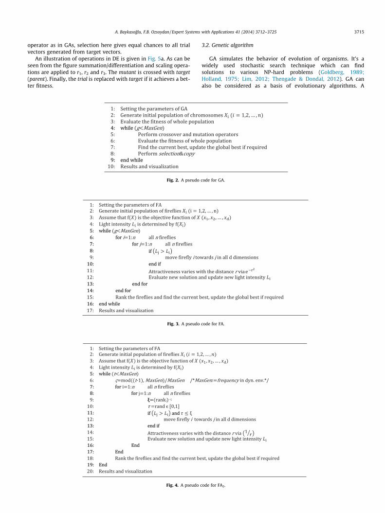
pseudo code representing the generic scheme of GA is illus-trated in Fig. 2.
In this study a single point crossover is used and one offspring isallowed to be generated. Offspring has a 0.5 chance to take the firstsegment from the first parent and second segment from the secondparent; and 0.5 chances to take the first segment from the secondparent and the second segment from the first parent.
Mutation operator assigns a new random number e [0,1] to thebits. Finally, roulette wheel selection is used as the selectionoperator.
A schematic illustration for obtaining new solutions usingcrossover and mutation for GA is given in Fig. 5.b. According to thisfigure, ch1 is crossed with the ch2 resulting in chtemp. Finally muta-tion operator is used for generating an offspring.
3.3. Firefly algorithm
FA is a population based metaheuristic algorithm which simu-lates the flashing and communication behavior of fireflies. It wasoriginally introduced by Yang (2008, 2009). In a typical FA algo-rithm the brightness of a firefly means how well the objective ofa solution is and brighter firefly (solution) attracts other fireflies.As the distance between fireflies increases, the attractiveness de-creases exponentially because of the light absorption of medium.A comprehensive survey of this new metaheuristic optimizer waspresented in the studies of Fister et al. (2013a), Fister, Yang, Brest,and Fister (2013b) and Yang and He (2013).
The application of the FA for dynamic environment is a newdeveloping research area and there are relatively fewer publishedpapers on this topic. Abshouri, Meybodi, and Bakhtiary (2011)hybridized FA with a learning automata for tuning the parametersof FA. Farahani, Nasiri, and Meybodi (2011) used a multi-popula-tion based FA by splitting the whole population into interactingsets of smaller swarms. Additionally each swarm was allowed tointeract locally and globally through an anti-convergence operatorto prevent an early convergence circumstance. Nasiri and Meybodi(2012) adopted an elitist approach within FA by keeping the bestsolution through generations. All these FA applications were testedon the well known multi-modal dynamic moving peaks problem(Branke, 1999) and the efficiency of the proposed FAs were shownby the authors.
Another dynamic optimization application of FA was presentedby Chai-ead, Aungkulanon, and Luangpaiboon (2011). A compari-son of FA and bees algorithm was performed on the various typesof noisy continuous mathematical functions with two variables.According to the findings of the study, authors concluded thatthe FA outperformed Bees algorithm.
Due to the structural properties (i.e. using floating numbers inits bits) of FA, this new optimizer is expected to perform more effi-ciently particularly on continuous environments and as it can beseen from above, whole literature of dynamic optimization for FAwas focused on this domain. However, the performance of FA ondynamic combinatorial problems still remains as a question mark.Additionally the most of real-life problems are combinatorial innature. To the best of our knowledge this paper constitutes the firststudy on the performance of FA on a dynamic combinatorial opti-mization problem.
FA has three main assumptions:
i. All fireflies are unisexual and every firefly attracts/getsattracted to every other firefly.
ii. The attractiveness of a firefly is directly proportional to thebrightness of the firefly (The brightness decreases as the dis-tance increases).
iii. They move randomly if they do not find a more attractivefirefly in adjacent regions.
A. Baykasoglu, F.B. Ozsoydan / Expert Systems with Applications 41 (2014) 3712–3725 3717
The distance between two fireflies (i and j) can simply be eval-uated as the Euclidean distance as stated below in Eq. (11), whereD is the dimension, xik is the kth dimension of the ith firefly.
rij ¼
ffiffiffiffiffiffiffiffiffiffiffiffiffiffiffiffiffiffiffiffiffiffiffiffiffiffiffiffiffiffiXD
k¼1
xik � xjk� �2
vuut ð11Þ
The attractiveness of a firefly decreases exponentially as the dis-tance increases. The attractiveness of a firefly at a distance cr is for-mulated as given in Eq. (12), where c is the light absorptioncoefficient, m is number which modifies the distance metric andb(0) is the attractiveness at 0 distance usually accepted as 1.
Fig. 5. (a) Obtaining a new proposal in DE (ri: ith randomly chosen individual) (b) Obtainischema of pair-wise comparison and movement in FA (fi: firefly with the ith rank).
Fig. 6. A visual illustration of n for the co
bðrÞ ¼ bð0Þe�cm
r m P 1 ð12Þ
Finally, movement of a firefly, i is attracted to another moreattractive (brighter) firefly j, is determined by Eq. (13)., wherea e [0, 1] is a user supplied scaling factor of randomness andw e [0, 1] is a random number.
xik ¼ xik þ bð0Þe�cr2 ðxjk � xikÞ þ aðw� 0:5Þ ð13Þ
A pseudo code for FA is given below in Fig. 3.Fig. 5c represents a schematic movement of fireflies. f1, f2 and f3
are assumed to have the 1st 2nd and 3rd rank, where the 1st rankrepresents the fittest firefly. According to this figure, f2 is only
ng a new solution in GA (chi: ith chromosome; chtemp: temporary chromosome) (c) A
rresponding rank though iterations.
3718 A. Baykasoglu, F.B. Ozsoydan / Expert Systems with Applications 41 (2014) 3712–3725
moved in the direction of f1, where f3 is moved to the positions ofboth f1 and f2. The fittest firefly f1 is allowed to fly randomly.
As it can be seen from the Fig. 3, FA performs a full pair-wisecomparison which can be time consuming. As a result the searchmight suffer from the computations of full pair-wise comparison.Another issue is that the exponential move function might deteri-orate the performance of FA unless the parameters are precisely setto their appropriate levels (Eq. (13)). It is widely reported in the lit-erature that c is assumed to be equal to 1; however, as the distancebetween fireflies increases, bð0Þe�cr2 approaches to zero whichmeans that such an assumption might cause fireflies be stuckedat a single position through generations. In order to prevent thiscircumstance, c can be set to very small values, however, obtainingthe appropriate level of c is not an easy task. Considering these twodrawbacks, an improved modification of FA called FA2 is presentedin this study.
Fig. 7. A pseudo code to obtain a solution from an encoded individual.
0.40.421121 00.73
2739 0.01
3.0163
0.20.294494 00.917
5917 0.57
6.5796
0.30.371771 00.842
8842 0.70
9.7039
0.410.4281028
Fig. 8. An example for solution encoding.
Table 2Parameters of the algorithms.
GA DE FA FA2
Maximum generation 10,000 10,000 10,000 10,000Frequency 1000 1000 1000 1000Population size 100 100 100 100Crossover rate 1.0 0.5 Na NaMutation rate 0.09 Na Na NaF (scaling factor) Na 0.8 Na Naa Na Na 0.9 0.9b(0) Na Na 1.0/0.35 1.0/0.35c Na Na 0.001 Na
Table 3Experimental results on stationary environments.
GA DE b(0) = 1.0
FA
# Best CPU (s) Best CPU (s) Best CPU (
Env1 3087,80 120,19 1776,80 110,37 1127,20 240,9Env2 3340,10 127,46 1877,05 107,45 1249,53 236,5Env3 3432,54 125,98 2112,76 115,21 1422,46 193,4Env4 3208,21 122,54 1859,10 99,64 1172,12 225,6Env5 3669,24 130,53 2233,41 112,98 1680,68 260,4Env6 3469,43 138,14 2000,46 107,56 1378,80 224,8Env7 3272,27 126,73 1858,90 102,64 1554,08 183,1Env8 3121,18 122,52 1565,68 109,49 1051,17 238,3Env9 2971,64 119,26 1442,65 103,52 1546,54 281,1Env10 3257,68 125,62 1888,60 101,71 1152,78 215,1
3.4. Improved firefly algorithm
According to FA2 a full pair-wise comparison is replaced with aspecialized comparison. The parameter 1 is changed from zero toapproximately one through iterations by using the Eq. (14), wheret is the iteration counter and maxGen is limit of iterations. It mustbe noted that maxGen is replaced with frequency in dynamic envi-ronment. Because 1 must be re-initialized as the dynamic change isdetected and then it adapts itself though the generations where thenew environment remains stationary.
1 ¼ modððt � 1Þ;maxGenÞ=maxGen ð14Þ
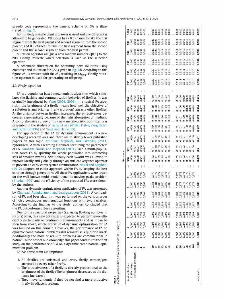
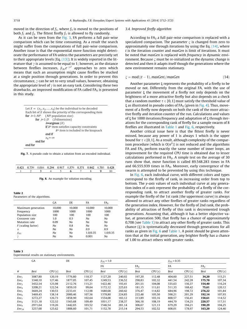
Another parameter n represents the probability of a firefly to bemoved or not. Differently from the original FA, with the use ofparameter n the movement of a firefly not only depends on thebrightness of a more attractive firefly but also depends on a checkthat a random number s 2 [0,1] must satisfy the threshold value ofn as illustrated in pseudo codes of FA2 (given in Fig. 4). Thus, move-ment of a firefly now depends on both the rank of the more attrac-tive firefly and iteration counter of the run. Calculations and valuesof n for 1000 iterations/frequency and adaptation of n through iter-ations for the corresponding rank of firefly for a sample swarm of 8fireflies are illustrated in Table 1 and Fig. 6, respectively.
Another critical issue here is that the fittest firefly is nevermissed, because any power of 1 is always 1 which is the upperbound for s 2 [0,1]. As a result, although complexity of the compar-ison procedure (which is O(n2)) is not reduced and the algorithmsFA and FA2 perform exactly the same number of inner loops, animprovement for the required CPU time is obtained due to lessercalculations performed in FA2. A simple test on the average of 30runs show that, move function is called 89.548.283 times in FAand 66.555.939 times in FA2. Moreover, early convergence of theswarm is attempted to be prevented by using this technique.
In Fig. 6, each individual curvei with different colors and typescorrespond to the firefly of ranki in increasing order from top tobottom. The y-axis values of each individual curve at any genera-tion index of x-axis represent the probability of a firefly of the cor-responding rank, to attract another firefly of greater ranks. Forexample the firefly of the 1st rank (the uppermost curve) is alwaysallowed to attract any other fireflies of greater ranks regardless ofthe generation index. However, for the firefly of 2nd rank, the prob-ability of attraction of firefly of this rank is decremented troughgenerations. Assuming that, although it has a better objective va-lue, at generation 500, that firefly has a chance of approximately0,708 (see Table 1) to attract any other firefly of greater ranks. Thischance (n) is systematically decreased through generations for allranks as given in Fig. 6 and Table 1. A point should be given atten-tion that at the initial generation, any brighter firefly has a chanceof 1.00 to attract others with greater ranks.
b(0) = 0.35
FA2 FA FA2
s) Best CPU (s) Best CPU (s) Best CPU (s)
2 197,20 112,48 404,60 227,51 34,20 115,212 298,83 102,32 441,54 242,28 175,70 107,341 201,55 104,08 535,63 156,37 154,40 116,243 181,15 111,61 511,33 168,42 75,61 120,122 376,47 114,82 684,96 198,72 276,22 101,845 222,48 105,50 598,21 201,29 192,14 107,932 313,89 103,16 800,57 156,41 158,61 114,527 366,18 108,19 444,79 134,25 220,57 117,514 306,67 121,13 679,29 194,21 190,29 104,254 294,53 102,52 608,01 178,97 163,20 124,46

A. Baykasoglu, F.B. Ozsoydan / Expert Systems with Applications 41 (2014) 3712–3725 3719
Due to the second drawback as mentioned before, the exponen-tial move function is replaced with a move function which is sim-ilar to Rahmaniani and Ghaderi (2013) in FA2. This function is givenin Eq. (15):
xik ¼ xik þ bð0Þð1=ðXþ rÞÞðxjk � xikÞ þ aðw� 0:5Þ ð15Þ
where X is very small number like 0.000001 in order to prevent thedivision by zero.
3.5. Solution representation
Although GA supports binary or permutation representation, it’sobvious that direct use of DE and FA to discrete search spaces yields
a. Env1
c. Env3
e. Env5
g. Env7
k. Env9
Fig. 9. (a-l) Convergence of GA, DE, FA and FA2
to illegal solutions. In other words using difference of vectors as inDE or moving operations as in FA is not appropriate in binary, per-mutation or other similar representation techniques. A mappingprocedure is required here in order to show that an item is assignedin the knapsack or not. Therefore in this study, priority basedencoding technique (Chitra & Subbaraj, 2012; Lotfi & Tavakkoli-Moghaddam, 2012) is used in order to represent a solution.
According to this representation technique, an individual hasbits as many as the number of items considered in the problem.The bits of the individuals simply hold unbounded continuousnumbers, representing the priority of each item to be included inthe knapsack. Additionally, the initial population is comprised ofrandom numbers bounded within the interval [0,1]. A pseudo code
b. Env2
.d Env4
.f Env6
.h Env8
l. Env10
on each stationary environment (b(0) = 1.0).
3720 A. Baykasoglu, F.B. Ozsoydan / Expert Systems with Applications 41 (2014) 3712–3725
for constructing a solution and a sample encoded solution arepresented in Figs. 7 and 8, respectively.
This technique always constructs feasible solutions andprevents infeasibility for both stationary and dynamic environ-ments. Thus, any repairing procedure is not required.
As it can be seen from Fig. 8, there are items indexed in a rangefrom 1 to 10 (2nd row), associated with random priorities (1strow). A higher number in 1st row provides a higher priority tothe corresponding item to be assigned unless it violates capacityconstraints. According to the priorities, items 5, 8, 2, 9, 6, 10, 1,7, 4, 3 are attempted to be assigned in sequence. Obviously, assum-ing that an assignment is performed, remaining capacities ofdimensions are updated. For instance, let item5 be assigned. Thenthe capacities of the knapsack dimensions are decreased as much
a. Env1
c. Env3
e. Env5
g. Env7
k. Env9
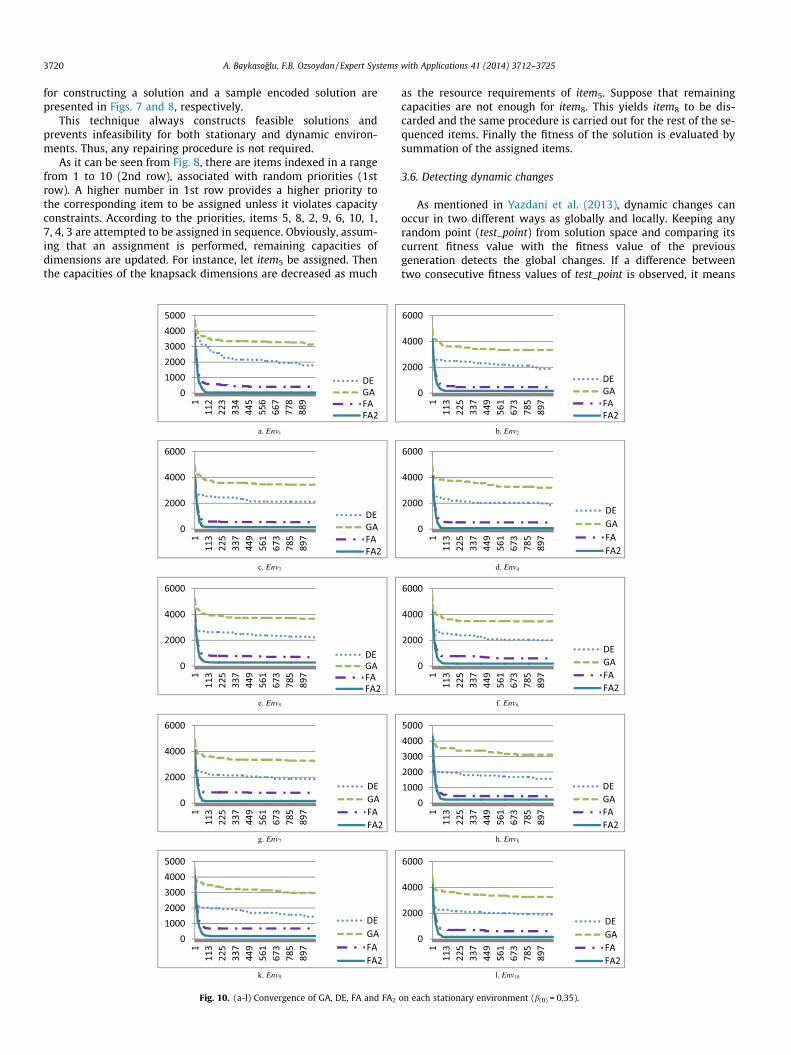
Fig. 10. (a-l) Convergence of GA, DE, FA and FA2
as the resource requirements of item5. Suppose that remainingcapacities are not enough for item8. This yields item8 to be dis-carded and the same procedure is carried out for the rest of the se-quenced items. Finally the fitness of the solution is evaluated bysummation of the assigned items.
3.6. Detecting dynamic changes
As mentioned in Yazdani et al. (2013), dynamic changes canoccur in two different ways as globally and locally. Keeping anyrandom point (test_point) from solution space and comparing itscurrent fitness value with the fitness value of the previousgeneration detects the global changes. If a difference betweentwo consecutive fitness values of test_point is observed, it means
b. Env2
.d Env4
.f Env6
.h Env8
l. Env10
on each stationary environment (b(0) = 0.35).
A. Baykasoglu, F.B. Ozsoydan / Expert Systems with Applications 41 (2014) 3712–3725 3721
that the environment has changed. It must be noted that suchdetection test is only appropriate for global changes. However,when a small local change occurs out of the vicinity of thetest_point, there’s a probability that the algorithm cannot detectthe change. Assuming that the change has occurred in the neigh-borhood of the optimum, then optimum solution of the previousgeneration can be used as the test_point. Yazdani et al. (2013) pre-sented a multi-swarm approach to evaluate fitness of theglobal_best_solutions of each swarm at the end of each iterationin order to detect such changes by making use of the advantageof multi-swarm based approaches.
In the present work, dynamic changes are assumed to occur forall of the objective’s and constraints’ coefficients similar to Brankeet al. (2006). Therefore, both solution vector which is constructedby using test_point and fitness value of the solution are expectedto change subsequent to dynamic event. However, it should benoted here that there is a probability for the solution vector toremain stationary. For this reason, at the end of each iteration, acheck on both solution vector and fitness value was performed asa detection test in this study. As a result, if a change is detectedbetween consecutive generations’ solution vector or fitness valueof the test_point, then algorithms react to that change as partialre-initializations to introduce diversity. Additionally, FA2
adapts the parameter n to increase ‘‘moving chance’’ of fireflies inthe new environment during the initial generations. It is shown bythe results that this approach has detected the changes at each run.
Table 4Experimental results on dynamic environment.
# GA best DE best FA best FA2 best
0.00 Re-initialization Env1 2495,10 1296,03 155,67 64,23Env2 2749,95 1224,54 288,59 300,15Env3 2731,41 1182,60 349,19 328,01Env4 2605,79 1119,09 447,14 411,19Env5 2797,49 1278,89 630,18 578,85Env6 2667,22 1191,80 502,85 485,89Env7 2519,34 1100,96 616,87 503,87
4. Experimental results
4.1. Experimental setup
As mentioned earlier, 10 different environments were gener-ated using the first test problem of mknapcb4.txt as a basis. Thebest error to optimum was used as the performance measure.According to this measure, the average values of the best solutionachieved for each of the environments on 30 runs are considered.The optimum of each environment was obtained using GAMSCPLEX solver. The parameters of DE, GA, FA and FA2 are set asshown in Table 2. Additionally, as the step size for FA is a criticalissue, b(0) is assumed to be equal to 1.0 and 0.35 separately, whichprovides a faster and slower convergence, respectively.
All tests were performed on a PC with hardware of 3.4 GHz pro-cessor and 4 GB RAM. Before representing the performance of thealgorithms on dynamic environment, experimental results on sta-tionary environments are discussed in the following subsection.
Env8 2734,75 1151,88 504,57 500,99Env9 2568,34 1106,50 709,11 652,72Env10 2553,12 1181,20 643,96 599,57
0.30 Re-initialization Env1 2499,10 1269,70 134,63 103,57Env2 2710,47 1235,21 336,65 330,56Env3 2747,88 1225,12 376,16 381,11Env4 2646,27 1158,47 456,20 391,05Env5 2778,76 1328,24 545,43 526,82Env6 2765,77 1288,36 509,54 514,92Env7 2607,60 1140,58 549,13 542,09Env8 2674,39 1226,11 456,16 488,97Env9 2551,32 1215,30 636,89 620,53Env10 2572,43 1263,64 543,16 531,78
0.70 Re-initialization Env1 2526,60 1277,60 147,73 74,83Env2 2735,42 1317,27 267,84 264,52Env3 2706,70 1359,98 270,08 251,71Env4 2589,56 1214,60 332,48 316,83Env5 2859,46 1438,12 466,20 405,06Env6 2813,77 1366,02 408,60 440,24Env7 2569,63 1223,63 408,68 388,43Env8 2715,51 1295,66 374,35 365,65Env9 2552,87 1314,21 471,37 514,24Env10 2586,08 1285,55 400,16 357,67
4.2. Results on stationary environment
Each of the dynamic environments is assumed as stationaryenvironments here. In other words, algorithms are assumed to bereinitialized with a random initial population for each of the dy-namic environments, and they are not allowed to gather and usethe information from the predecessor environment. Results interms of average of the best error from optimum are illustratedin Table 3.
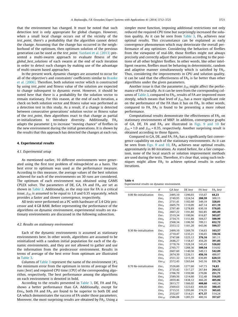
Columns of Table 3 represent the name of the environment (#),the minimum error from the optimum in terms of average of fiveruns (best) and required CPU time (CPU) of the corresponding algo-rithm, respectively. The best performance among the algorithmson each environment is denoted in bold.
According to the results presented in Table 3, DE, FA and FA2
shows a better performance than GA. Additionally, except forEnv9, both FA and FA2 are found to be superior to both DE andGA which demonstrates the success of FA under those parameters.Moreover, the most surprising results are obtained by FA2. Using a
simpler move function, imposing additional restrictions not onlyreduced the required CPU time but surprisingly increased the solu-tion quality. As it can be seen from Table 3, FA2 achieves nearoptimal results. This circumstance can be explained as earlyconvergence phenomenon which may deteriorate the overall per-formance of any optimizer. Considering the behaviors of firefliesfrom the viewpoint of real-life, those fireflies might not alwaysprecisely and correctly adjust their positions according to the posi-tions of all other brighter fireflies. In other words, like other intel-ligent swarms, fireflies must be behaving in deterministic, randomand adaptive manner simultaneously which is satisfied by FA2.Thus, considering the improvements in CPU and solution quality,it can be said that the effectiveness of FA2 is far better than otheralgorithms under the given parameters.
Another issue is that the parameter b(0) might affect the perfor-mance of FA crucially. As it can be seen from the corresponding col-umns of Table 3, compared to FA2, results of FA are improved moresteeply, which means that level of b(0) has a more significant roleon the performance of the FA than it has on FA2. In other words,compared to FA, FA2 is found to be presenting a more robustperformance.
Computational results demonstrate the effectiveness of FA2 onstationary environments of MKP. In addition, convergence graphsof GA, DE, FA and FA2 are illustrated in Figs. 9 and 10 forb(0) = 1.0 and b(0) = 0.35, respectively. Another surprising result isobtained according to those figures.
Compared to GA, DE, and FA; FA2 has a significantly fast conver-gence capability on each of the stationary environments. As it canbe seen from Figs. 9 and 10, FA2 achieves near optimal results,approximately in 80 iterations. As stated before, for a fair compar-ison, none of the local search or solution improvement methodsare used during the tests. Therefore, it’s clear that, using such tech-niques might allow FA2 to achieve optimal results in earlieriterations.

3722 A. Baykasoglu, F.B. Ozsoydan / Expert Systems with Applications 41 (2014) 3712–3725
Following subsection is devoted to the analysis of the perfor-mances of GA, DE, FA and FA2 on dynamic environments.
4.3. Results on dynamic environment
Computational results for stationary environments demon-strate the effectiveness of FA2. However, these results might bemisleading for dynamic environments possibly because of lack ofthe capability of tracking the changing optima. For dynamic
a
b
c
Fig. 11. Convergence of GA, DE, FA and FA2 on dynamic env
environments, an effective algorithm is expected to quickly adaptto new environments and track the changing optima. Moreover,diversity must be introduced or maintained through evaluationsfor adaptation to dynamic changes. Particularly just after thedynamic event is triggered, an effective algorithm is expected todetect the change and react to it. For this reason, tests on dynamicenvironments are performed by reinitializing and randomlyrestarting 0%, 30% and 70% of the population when a dynamicchange is detected. This approach can be considered as partial
ironments with (a) 0% (b) 30% (c) 70% re-initialization.
A. Baykasoglu, F.B. Ozsoydan / Expert Systems with Applications 41 (2014) 3712–3725 3723
random restarts, which is a trade-off between keeping thegathered evolutionary information through generations andemploying some random scouts in the swarm to explore the newenvironment by allowing them to reinitialize their individualmemories. Additionally, FA2 adjusts the parameter n when adynamic change is detected and readapts it through generationsof the new environment. Thus, two common concepts of dynamicoptimization namely, introducing and maintaining diversity aresimultaneously implemented in FA2.
As demonstrated in the previous subsection, both FA and FA2
achieves betters results for b(0) = 0.35. Therefore tests on dynamicenvironments are performed using this assumption. Results, interms of the best average of errors of 30 runs for each algorithmwith 0%, 30% and 70% restarts are presented in Table 4.
According to Table 4 where the algorithms are not allowed to bereinitialized, DE, FA and FA2 are found to be more effective thanGA. Additionally, FA2 achieves the best results although an incre-ment in the error from optimum is apparent compared to the re-sults on stationary environment. However, if the algorithms areallowed to use the 0.30 and 0.70 of the previously gathered infor-mation, another surprising result is obtained.
It’s obvious that results are improved for both FA and FA2 whichmeans that the performances of both algorithms increase as therate of introduced diversity is increased. As a result, FA becomescompetitive with FA2. However, apparently this is not valid forGA and DE. It can be seen that GA performs an insensitive behaviorto the rate of the diversity introduced whereas a slight decrementfor the performance of DE is observed based on the results repre-sented in Table 4.
Convergence graphs of the GA, DE, FA and FA2, for the tests with0.00, 0.30 and 0.70 restarts of the population are illustrated inFig. 11a–c, respectively. It is apparent from this figure that, asthe introduced diversity increases, an obvious increment for theseverity of the deviance just after a change is observed for bothFA and FA2.
4.4. Statistical verification
In this subsection, a statistical verification is performed to provewhat intuition suggests in the findings of the Sections 4.2 and 4.3.Therefore an initial analysis is scheduled to see whether a mean-ingful difference among algorithms exists. Friedman Test(Friedman, 1937, 1940) which is a non-parametric test, applicableto multiple classifiers is performed for this purpose. Subsequent toinitial results, a paired t-test analysis is carried out between eachpair of algorithms.
For tests on stationary and dynamic environments data set iscomprised of mean errors from optimum on 5 and 30 runs,
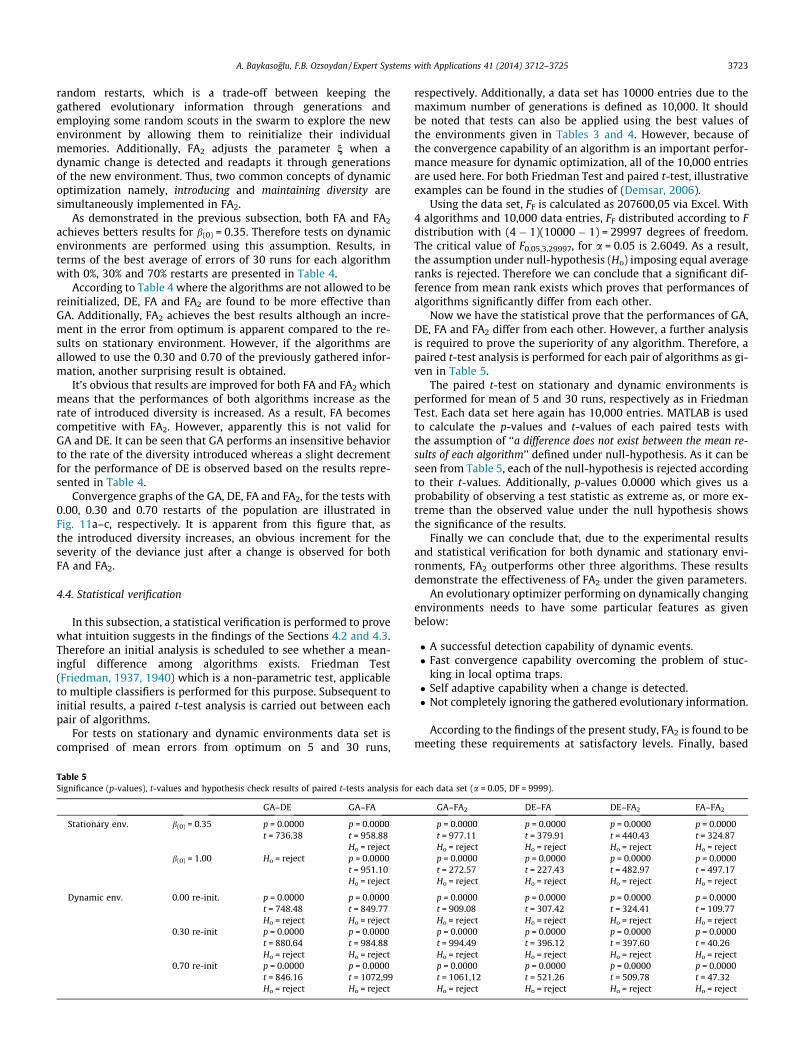
Table 5Significance (p-values), t-values and hypothesis check results of paired t-tests analysis for
GA–DE GA–FA
Stationary env. b(0) = 0.35 p = 0.0000 p = 0.0000t = 736.38 t = 958.88
Ho = rejectb(0) = 1.00 Ho = reject p = 0.0000
t = 951.10Ho = reject
Dynamic env. 0.00 re-init. p = 0.0000 p = 0.0000t = 748.48 t = 849.77Ho = reject Ho = reject
0.30 re-init p = 0.0000 p = 0.0000t = 880.64 t = 984.88Ho = reject Ho = reject
0.70 re-init p = 0.0000 p = 0.0000t = 846.16 t = 1072,99Ho = reject Ho = reject
respectively. Additionally, a data set has 10000 entries due to themaximum number of generations is defined as 10,000. It shouldbe noted that tests can also be applied using the best values ofthe environments given in Tables 3 and 4. However, because ofthe convergence capability of an algorithm is an important perfor-mance measure for dynamic optimization, all of the 10,000 entriesare used here. For both Friedman Test and paired t-test, illustrativeexamples can be found in the studies of (Demsar, 2006).
Using the data set, FF is calculated as 207600,05 via Excel. With4 algorithms and 10,000 data entries, FF distributed according to Fdistribution with (4 � 1)(10000 � 1) = 29997 degrees of freedom.The critical value of F0.05,3,29997, for a = 0.05 is 2.6049. As a result,the assumption under null-hypothesis (Ho) imposing equal averageranks is rejected. Therefore we can conclude that a significant dif-ference from mean rank exists which proves that performances ofalgorithms significantly differ from each other.
Now we have the statistical prove that the performances of GA,DE, FA and FA2 differ from each other. However, a further analysisis required to prove the superiority of any algorithm. Therefore, apaired t-test analysis is performed for each pair of algorithms as gi-ven in Table 5.
The paired t-test on stationary and dynamic environments isperformed for mean of 5 and 30 runs, respectively as in FriedmanTest. Each data set here again has 10,000 entries. MATLAB is usedto calculate the p-values and t-values of each paired tests withthe assumption of ‘‘a difference does not exist between the mean re-sults of each algorithm’’ defined under null-hypothesis. As it can beseen from Table 5, each of the null-hypothesis is rejected accordingto their t-values. Additionally, p-values 0.0000 which gives us aprobability of observing a test statistic as extreme as, or more ex-treme than the observed value under the null hypothesis showsthe significance of the results.
Finally we can conclude that, due to the experimental resultsand statistical verification for both dynamic and stationary envi-ronments, FA2 outperforms other three algorithms. These resultsdemonstrate the effectiveness of FA2 under the given parameters.
An evolutionary optimizer performing on dynamically changingenvironments needs to have some particular features as givenbelow:
� A successful detection capability of dynamic events.� Fast convergence capability overcoming the problem of stuc-
king in local optima traps.� Self adaptive capability when a change is detected.� Not completely ignoring the gathered evolutionary information.
According to the findings of the present study, FA2 is found to bemeeting these requirements at satisfactory levels. Finally, based
each data set (a = 0.05, DF = 9999).
GA–FA2 DE–FA DE–FA2 FA–FA2
p = 0.0000 p = 0.0000 p = 0.0000 p = 0.0000t = 977.11 t = 379.91 t = 440.43 t = 324.87Ho = reject Ho = reject Ho = reject Ho = rejectp = 0.0000 p = 0.0000 p = 0.0000 p = 0.0000t = 272.57 t = 227.43 t = 482.97 t = 497.17Ho = reject Ho = reject Ho = reject Ho = reject
p = 0.0000 p = 0.0000 p = 0.0000 p = 0.0000t = 909.08 t = 307.42 t = 324.41 t = 109.77Ho = reject Ho = reject Ho = reject Ho = rejectp = 0.0000 p = 0.0000 p = 0.0000 p = 0.0000t = 994.49 t = 396.12 t = 397.60 t = 40.26Ho = reject Ho = reject Ho = reject Ho = rejectp = 0.0000 p = 0.0000 p = 0.0000 p = 0.0000t = 1061,12 t = 521.26 t = 509.78 t = 47.32Ho = reject Ho = reject Ho = reject Ho = reject

3724 A. Baykasoglu, F.B. Ozsoydan / Expert Systems with Applications 41 (2014) 3712–3725
upon the experimental results, it can be concluded that FA2 can beconsidered as an effective optimization algorithm on both staticand dynamic environments.
5. Conclusions
This paper presents a comparative analysis of the performancesof GA, DE and FA on both static and dynamic multidimensionalknapsack problems. To the best of our knowledge this paper con-stitutes the first paper on the combinatorial dynamic optimizationof FA.
One of the important contributions of the study is the develop-ment of FA2, which is designed for a more realistic reflection of thebehaviors of fireflies. FA2 requires less computational time; more-over it achieves significantly superior results on both static anddynamic multidimensional knapsack problems. Particularly onstationary environments, FA2 obtains near optimal results with asignificantly faster convergence capability. Thus, it can be said thatFA2 was found to be more effective compared to GA, DE and FA forthe problems studied in this paper.
Because it’s a relatively new metaheuristic algorithm, the per-formance of pure FA along with the performances of pure GA andDE is also presented through this paper. In other words, anyenhancement procedure is avoided as far as possible for a fair anal-ysis. However, a research for the effects of such procedures mightbe scheduled as a future work. Additionally, the performance ofFA2 might be analyzed through different dynamic problems. Partic-ularly, continuous dynamic optimization where moving peaksexist might be an appropriate candidate for such an analysis.
As another future work, a comparative study with the sate-of-the-art algorithms such as jDE, SaDE, ‘‘HyperMutation GA’’ and‘‘GA with Random Immigrants’’ which were designed particularlyfor dynamic optimization problems can be carried out.
References
Abshouri, A., Meybodi, M., & Bakhtiary, A. (2011). New firefly algorithm based onmulti swarm & learning automata in dynamic environments. In IEEE proceedings(pp. 73–77).
Baykasoglu, A., & Durmus�oglu, Z. D. U. (2011). Dynamic optimization in a dynamicand unpredictable world. In 2011 Proceedings of PICMET ‘11: Technologymanagement in the energy-smart world (PICMET), July 31–August 4, 2011 (pp.2312–2319). Portland, OR, USA: Hilton Portland and Executive Tower.
Baykasoglu, A., & Durmus�oglu, Z. D. U. (2013). A classification scheme for agentbased approaches to dynamic optimization. Artificial Intelligence Review. http://dx.doi.org/10.1007/s10462-011-9307-x.
Bosman, P. A. N. (2005). Learning, anticipation and time-deception in evolutionaryonline dynamic optimization. In Proceedings of the 2005 workshops on geneticand evolutionary computation (pp. 39–47).
Bosman, P. A. N., & Poutrè, H. L. (2007). Learning and anticipation in online dynamicoptimization with evolutionary algorithms: The stochastic case. In Proceedingsof the 2007 genetic and evolutionary computation conference (pp. 1165–1172).
Branke, J. (1999). Memory enhanced evolutionary algorithms for changingoptimization problems. In Proceedings of the congress on evolutionarycomputation 99 (Vol. 3, pp. 1–8).
Branke, J. (2002). Evolutionary optimization in dynamic environments. Dordrecht:Kluwer.
Branke, J., Kau, T., Schmidt, C., & Schmeck, H. (2000). A multi-population approachto dynamic optimization problems. In I. E. Parmee (Ed.), Evolutionary design andmanufacture (pp. 299–308). London: Springer-Verlag.
Branke, J., Orbayı, M., & Uyar, S�. (2006). The role of representations in dynamicknapsack problems. In F. Rothlauf, J. Branke, S. Cagnoni, E. Costa, C. Cotta, R.Drechsler, E. Lutton, P. Machado, J. H. Moore, J. Romero, G. D. Smith, G. Squillero,& H. Takagi (Eds.), Applications of evolutionary computing (pp. 764–775). BerlinHeidelberg: Springer Verlag.
Brest, J., Korošec, P., Šilc, J., Zamuda, A., Boškovic, B., & Maucec, M. S. (2013).Differential evolution and differential ant-stigmergy on dynamic optimisationproblems. International Journal of Systems Science, 44(4), 663–679.
Brest, J., Greiner, S., Boškovic, B., Mernik, M., & Zumer, V. (2006). Self adaptingcontrol parameters in differential evolution: A comparative study on numericalbenchmark problems. IEEE Transactions on Evolutionary Computation, 10,646–657.
Chai-ead, N., Aungkulanon, P., & Luangpaiboon, P. (2011). Bees and fireflyalgorithms for noisy non-linear optimization problems. In Proceedings of the
international multi conference of engineering and computer scientists (Vol. 2, pp.1449–1454).
Chitra, C., & Subbaraj, P. (2012). A nondominated sorting genetic algorithm solutionfor shortest path routing problem in computer networks. Expert Systems withApplications, 39, 1518–1525.
Cobb, H. G. (1990). An investigation into the use of hypermutation as an adaptiveoperator in genetic algorithms having continuous, time dependantnonstationary environments. Technical Report, Naval Research Laboratory,WA, USA.
Das, S., & Suganthan, P. N. (2011). Differential evolution: A survey of the state-of-the-art. IEEE Transactions on Evolutionary Computation, 15, 4–31.
Dean, B. C., Goemans, M. X., & Vondrák, J. (2008). Approximating the stochasticknapsack problem: The benefit of adaptivity. Mathematics of OperationsResearch, 33(4), 945–964.
Demsar, J. (2006). Statistical comparisons of classifiers over multiple data sets.Journal of Machine Learning Research, 7, 1–30.
Farahani, S., Nasiri, B., & Meybodi, M. (2011). A multi swarm based firefly algorithmin dynamic environments. In The third international conference on signalprocessing systems (ICSPS2011) (Vol. 3, pp. 68–72).
Farina, M., Deb, K., & Amato, P. (2004). Dynamic multiobjective optimizationproblems: Test cases, approximations, and applications. IEEE Transactions onEvolutionary Computation, 8(5), 425–442.
Fister, I., Fister, I., Jr., Yang, X.-S., & Brest, J. (2013a). A comprehensive review offirefly algorithms. Swarm and Evolutionary Computation, 13, 34–46.
Fister, I., Yang, X.-S., Brest, J., & Fister, I. Jr., (2013b). Modified firefly algorithm usingquaternion representation. Expert System with Applications, 40, 7220–7230.
Friedman, M. (1937). The use of ranks to avoid the assumption of normality implicitin the analysis of variance. Journal of the American Statistical Association, 32,675–701.
Friedman, M. (1940). A comparison of alternative tests of significance for theproblem of m rankings. Annals of Mathematical Statistics, 11, 86–92.
Goldberg, D. E. (1989). Genetic algorithms in search, optimization, and machinelearning. Reading, Massachusetts: Addison-Wesley.
Goldberg, D. E., & Smith, R. E. (1987). Nonstationary function optimization usinggenetic algorithms with dominance and diploidy. In J. J. Grefenstette (Ed.),Second international conference on genetic algorithms (pp. 59–68). New Jersey:Lawrence Erlbaum Associates.
Grefenstette, J. J. (1992). Genetic algorithms for changing environments. In R.Manner & B. Manderick (Eds.). Proceedings of the second international conferenceon parallel problem solving from nature (Vol. 2, pp. 137–144). Amsterdam:Elsevier.
Hadad, B. S., & Eick, C. F. (1997). Supporting polyploidy in genetic algorithms usingdominance vectors. In P. J. Angeline, R. G. Reynolds, J. R. McDonnell, & R.Eberhart (Eds.), Evolutionary programming VI (pp. 223–234). Berlin: Springer.
Hartman, J. C., & Perry, T. C. (2006). Approximating the solution of a dynamic,stochastic multiple knapsack problem. Control and Cybernetics, 35(3),535–550.
Holland, J. H. (1975). Adaptation in natural and artificial systems. Michigan AnnArbor: University of Michigan Press.
Jin, Y., & Branke, J. (2005). Evolutionary optimization in uncertain environments – Asurvey. IEEE Transactions on Evolutionary Computation, 9(3), 303–317.
Karaman, A., & Uyar, A. S. E. (2004). A novel change severity detection mechanismfor the dynamic 0/1 knapsack problem. In Proceedings of mendel 2004: 10thinternational conference on soft computing. Zakopane, Poland, June 7–11.
Karaman, A., Uyar, S�., & Eryigit, G. (2005). The memory indexing evolutionaryalgorithm for dynamic environments. In F. Rothlauf, J. Branke, S. Cagnoni, D. W.Corne, R. Drechsler, & Y. Jin (Eds.), Applications of evolutionary computing(pp. 563–573). Berlin Heidelberg: Springer Verlag.
Karve, A., Kimbrel, T., Pacifici, G., Spreitzer, M., Steinder, M., & Sviridenko, M., et al.(2006). Dynamic placement for clustered web applications. In WWW2006.Edinburgh, UK.
Kellerer, H., Pferschy, U., & Pisinger, D. (2004). Knapsack problems. Berlin: Springer.Kimbrel, T., Steinder, M., Sviridenko, M., & Tantawi, A. (2005). Dynamic application
placement under service and memory constraints. In S. E. Nikoletseas (Ed.),Experimental and efficient algorithms (pp. 391–402). Heidelberg: SpringerVerlag.
Kleywegt, A. J., & Papastavrou, J. D. (1998). The dynamic and stochastic knapsackproblem. Operations Research, 46(1), 17–35.
Kleywegt, A. J., & Papastavrou, J. D. (2001). The dynamic and stochastic knapsackproblem with random sized items. Operations Research, 49(1), 26–41.
Li, C., & Yang, S. (2008). A generalized approach to construct benchmark problemsfor dynamic optimization. In X. Li, M. Kirley, M. Zhang, D. Green, V. Ciesielski, H.Abbass, Z. Michalewicz, T. Hendtlass, K. Deb, K. C. Tan, J. Branke, & Y. Shi (Eds.),Simulated evolution and learning (pp. 391–400). Heidelberg Berlin: SpringerVerlag.
Liekens, A. M. L. (2005). Evolution of finite populations in dynamic environments. Ph.D.thesis, Technische Universitat, Eindhoven.
Lim, T. Y. (2012). Structured population genetic algorithms: A literature survey.Artificial Intelligence Review. http://dx.doi.org/10.1007/s10462-012-9314-6(http://link.springer.com/article/10.1007%2Fs10462-012-9314-6).
Lotfi, M. M., & Tavakkoli-Moghaddam, R. (2012). A genetic algorithm using priority-based encoding with new operators for fixed charge transportation problems.Applied Soft Computing, 13, 2711–2726.
Nasiri, B., & Meybodi, M. (2012). Speciation based firefly algorithm for optimizationin dynamic environments. International Journal of Artificial Intelligence, 8,118–132.

A. Baykasoglu, F.B. Ozsoydan / Expert Systems with Applications 41 (2014) 3712–3725 3725
Morrison, R. W. (2004). Designing evolutionary algorithms for dynamic environments.Berlin: Springer.
Qin, A. K., Huang, V. L., & Suganthan, P. N. (2009). Differential evolution algorithmwith strategy adaptation for global numerical optimization. IEEE Transactions onEvolutionary Computation, 13, 398–417.
Rahmaniani, R., & Ghaderi, A. (2013). A combined facility location and networkdesign problem with multi-type of capacitated links. Applied MathematicalModelling, 37, 6400–6414.
Rohlfshagen, P., Lehre, P. K., & Yao, X. (2009). Dynamic evolutionary optimisation:An analysis of frequency and magnitude of change. In Proceedings of the 2009genetic and evolutionary computation conference, July 8–12 (pp. 1713–172).Montréal Québec, Canada.
Rohlfshagen, P., & Yao, X. (2008). Attributes of dynamic combinatorial optimization.Lecture Notes in Computer Science, 5361, 442–451.
Rohlfshagen, P., & Yao, X. (2011). Dynamic combinatorial optimisationproblems: An analysis of the subset sum problem. Soft Computing, 15,1723–1734.
Rossi, C., Barrientos, A., & del Cerro, J. (2007). Two adaptive mutation operators foroptima tracking in dynamic optimization problems with evolution strategies. InProceedings of the 2007 annual conference on genetic and evolutionarycomputation, July 7–11 (pp. 697–704). London, England, United Kingdom.
Storn, R., & Price, K. (1995). Differential evolution-a simple and efficient adaptivescheme for global optimization over continuous spaces. Technical Report TR-95-012, ICSI, March 1995 (Available via ftp from ftp.icsi.berkeley.edu/pub/techreports/1995/tr-95-012.ps.Z).
Thengade, A., & Dondal, R. (2012). Genetic algorithm – Survey paper. IJCAproceedings on national conference on recent trends in computing (Vol. 5,pp. 25–29). NY, USA: Published by Foundation of Computer Science.
Thierens, D. (2002). Adaptive mutation rate control schemes in genetic algorithms.Evolutionary Computation, 1, 980–985.
Ursem, R. K., Krink, T., Jensen, M. T., & Michalewicz, Z. (2002). Analysis and modelingof control tasks in dynamic systems. IEEE Transactions on EvolutionaryComputation, 6(4), 378–389.
van Hemert, J. I., van Hoyweghen, C., Lukschandl, E., & Verbeeck, K. (2001). A‘‘futurist’’ approach to dynamic environments. In J. Branke & T. Bäck (Eds.),
Proceedings of the workshop on evolutionary algorithms for dynamic optimizationproblems at the genetic and evolutionary computation conference (pp. 35–38).
Weicker, K. (2003). Evolutionary algorithms and dynamic optimization problems. DerAndere: Verlag.
Wilke, C. O. (1999). Evolutionary dynamics in time-dependent environments. Ph.D.thesis, Ruhr-Universität, Bochum.
Yang, S. (2003). Non-stationary problem optimization using the primaldual geneticalgorithms. Evolutionary Computation, 3, 2246–2253.
Yang, S. (2005). Memory-based immigrants for genetic algorithms in dynamicenvironments. Proceedings of the 2005 genetic and evolutionary computationconference (Vol. 2, pp. 1115–1122). New York: ACM Press.
Yang, S. (2006). Associative memory scheme for genetic algorithms in dynamicenvironments. In F. Rothlauf, J. Branke, S. Cagnoni, E. Costa, & C. Cotta (Eds.),Applications of evolutionary computing (pp. 788–799). Berlin, Heidelberg:Springer-Verlag.
Yang, S., Ong, Y. S., & Jin, Y. (Eds.), (2007). Evolutionary computation in dynamicand uncertain environments. Berlin: Springer. http://www.springer.com/engineering/computational+intelligence+and+complexity/book/978-3-540-49772-1.
Yang, X.-S. (2008). Nature-inspired metaheuristic algorithm. Frome, Somerset:Luniver Press.
Yang, X.-S. (2009). Firefly algorithms for multimodal optimization. In Stochasticalgorithms: Foundations and applications, SAGA 2009. Lecture notes incomputer sciences (Vol. 5792, pp. 169–178).
Yang, X.-S., & He, X. (2013). Firefly algorithm: Recent advances and applications.International Journal of Swarm Intelligence, 1, 36–50.
Yazdani, D., Nasiri, B., Sepas-Moghaddam, A., & Meybodi, M. R. (2013). A novelmulti-swarm algorithm for optimization in dynamic environments based onparticle swarm optimization. Applied Soft Computing, 13, 2144–2158.
Web reference
(http://people.brunel.ac.uk/�mastjjb/jeb/orlib/files/mknapcb4.txt) Last access:02.10.2013.