Expert Systems With Applications 107 (2018) 32–44

Contents lists available at ScienceDirect

Expert Systems With Applications

journal homepage: www.elsevier.com/locate/eswa

Recognizing human activity in mobile crowdsensing environment

using optimized k -NN algorithm

Alaa Tharwat a , e , Hani Mahdi b , Mohamed Elhoseny

c , e , 1 , ∗, Aboul Ella Hassanien

d , e

a Faculty of Computer Science and Engineering, Frankfurt University of Applied Sciences, 60318 Frankfurt am Main, Germany. b Faculty of Engineering, Ain Shams University, Cairo, Egypt c Faculty of Computers and Information, Mansoura University, Mansoura, Egypt d Faculty of Computers and Information, Cairo Univeristy, Cairo, Egypt e Scientific Research Group in Egypt (SRGE), Cairo University, Cairo, Egypt

a r t i c l e i n f o

Article history:

Received 26 December 2017

Revised 1 April 2018

Accepted 11 April 2018

Available online 12 April 2018

Keywords:

Mobile crowd sensing

Human activities

Particle swarm optimization (PSO)

Optimization algorithms

k -Nearest Neighbor ( k -NN)

Classification

Parameter optimization

Swarm intelligent

a b s t r a c t

Mobile crowdsensing is a recent model in which a group of mobile users uses their smart devices such

as smartphones or wearable devices to cooperatively perform a large-scale sensing task. In this paper,

a novel model will be introduced for recognizing/classifying human activities that were collected from

sensor units on the chest, legs, and arms. The proposed model employed the k -Nearest Neighbor ( k -NN)

classifier which is one of the most common classifiers. k -NN has only one parameter, k , to determine

the number of selected nearest neighbors to the test or unknown samples for predicting the class la-

bels of the unknown samples. Searching for the value of k which has a great impact on the classification

performance is difficult especially with high dimensional data. This paper employs the Particle Swarm

Optimization (PSO) algorithm to search for the optimal value of the k parameter in the k -NN Classifier.

This paper shows first experimentally how the PSO in the proposed algorithm searches for the optimal

value of k parameter to reduce the misclassification rate of the k -NN classifier. Then, in the second ex-

periment, ten standard datasets are utilized to benchmark the performance of the proposed algorithm.

For verification, the results of the PSO- k NN algorithm are compared with two well-known algorithms:

Genetic Algorithm (GA) and Ant Bee Colony Optimization (ABCO). In the third experiment, the proposed

PSO- k NN algorithm was employed for recognizing human activities. The experimental results proved that

the PSO- k NN algorithm is able to find the optimal or near optimal value(s) of the k parameter which en-

hances the accuracy of k -NN classifier. The results also demonstrated lower error rates compared when

GA and ABCO algorithms.

© 2018 Elsevier Ltd. All rights reserved.

e

a

w

s

W

o

a

d

v

1. Introduction

Mobile crowdsensing is one of the new sensing models in

which a group of mobile users utilizes their smart devices such

as mobiles to cooperatively perform a large-scale sensing task

( Bedogni, Di Felice, & Bononi, 2012; Montori, Bedogni, Di Chiap-

pari, & Bononi, 2016; Tomasini, Mahmood, Zambonelli, Brayner, &

Menezes, 2017 ). Hence, crowdsensing enables carrying on exten-

sive measurements covering a large area with limited costs. How-

∗ Corresponding author at: Scientific Research Group in Egypt (SRGE), Egypt.

E-mail addresses: engalaatharwat@hotmail.com (A. Tharwat),

hani.mahdi@eng.asu.edu.eg (H. Mahdi), Mohamed_elhoseny@mans.edu.eg (M.

Elhoseny), aboitcairo@gmail.com (A.E. Hassanien).

URL: http://www.egyptscience.net (M. Elhoseny), http://www.egyptscience.net

(A.E. Hassanien) 1 Faculty of Computer Science and Engineering, Frankfurt University of Applied

Sciences, 60318 Frankfurt am Main, Germany

c

fi

k

E

m

i

t

h

https://doi.org/10.1016/j.eswa.2018.04.017

0957-4174/© 2018 Elsevier Ltd. All rights reserved.

ver, crowdsensing has some limitations such as the signal cover-

ge area, battery lifetime, and the heterogeneity of the used hard-

are ( Elhoseny, Farouk, Zhou, Wang, Abdalla, & Batle, 2017; Elho-

eny, Tharwat, Farouk, & Hassanien, 2017; Elhoseny et al., 2015 ).

ith the rapid advances in mobiles and smartphones technol-

gy, the size, processing time, weight and cost of commercially

vailable inertial sensors have decreased considerably over the last

ecade ( Ahmed et al., 2010; Titterton & Weston, 2004 ). This ad-

ancement in mobile technology gives the ability to acquire lo-

al knowledge using sensor-enhanced mobile devices such as traf-

c conditions, surrounding context, noise level, location, and this

nowledge can be shared ( Elhoseny, Elminir, Riad, & Yuan, 2014;

lhoseny, Tharwat, Yuan, & Hassanien, 2018 ). However, automatic

onitoring of human activities is one of the recent applications

n this field ( Montori et al., 2016 ). There are many challenges in

his research area such as collecting data, managing big data, and

andling noisy data ( Barshan & Yüksek, 2013; Carbajo, Carbajo,

A. Tharwat et al. / Expert Systems With Applications 107 (2018) 32–44 33

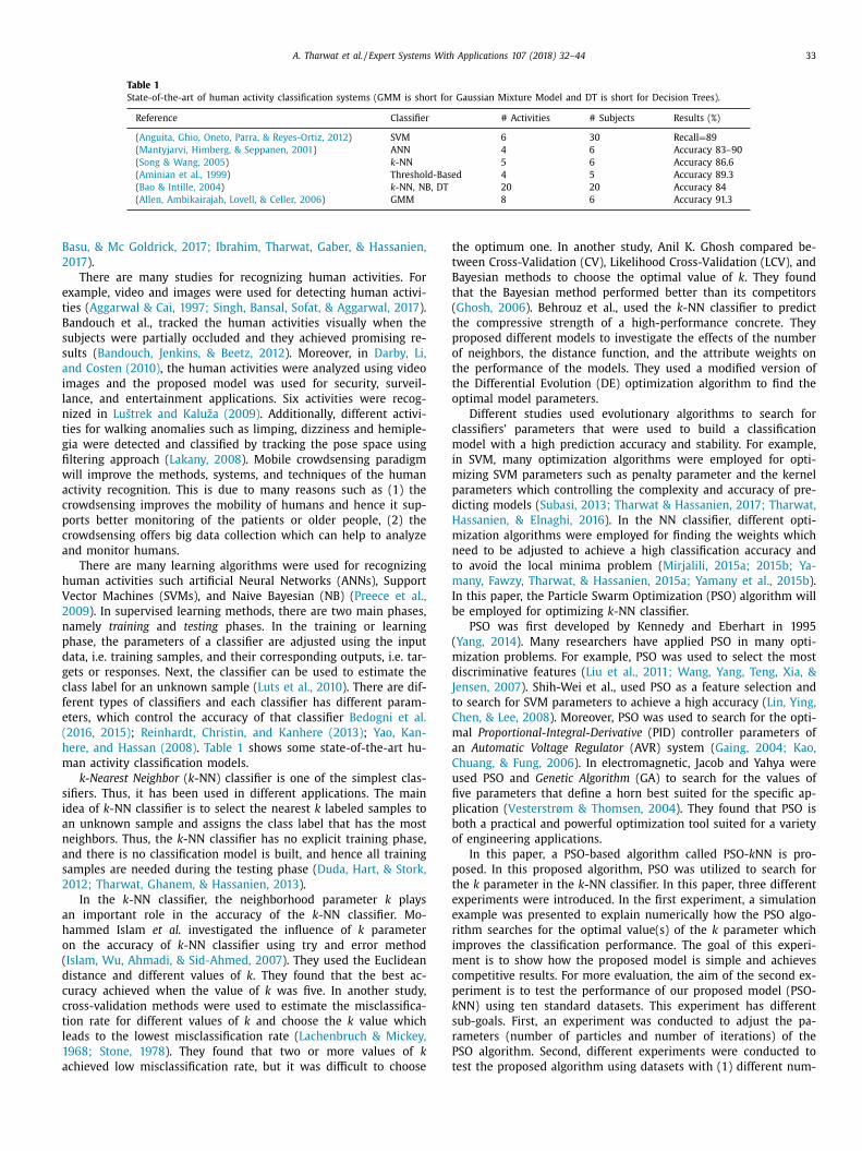
Table 1

State-of-the-art of human activity classification systems (GMM is short for Gaussian Mixture Model and DT is short for Decision Trees).

Reference Classifier # Activities # Subjects Results (%)

( Anguita, Ghio, Oneto, Parra, & Reyes-Ortiz, 2012 ) SVM 6 30 Recall = 89

( Mantyjarvi, Himberg, & Seppanen, 2001 ) ANN 4 6 Accuracy 83–90

( Song & Wang, 2005 ) k -NN 5 6 Accuracy 86.6

( Aminian et al., 1999 ) Threshold-Based 4 5 Accuracy 89.3

( Bao & Intille, 2004 ) k -NN, NB, DT 20 20 Accuracy 84

( Allen, Ambikairajah, Lovell, & Celler, 2006 ) GMM 8 6 Accuracy 91.3

B

2

e

t

B

s

s

a

i

l

n

t

g

fi

w

a

c

p

c

a

h

V

2

n

p

d

g

c

f

e

(

h

m

s

i

a

n

a

s

2

a

h

o

(

d

c

c

t

l

1

a

t

t

B

t

(

t

p

o

t

t

o

c

m

i

m

p

d

H

m

n

t

m

I

b

(

m

d

J

t

C

m

a

C

u

fi

p

b

o

p

t

e

e

r

i

m

c

p

k

s

r

P

t

asu, & Mc Goldrick, 2017; Ibrahim, Tharwat, Gaber, & Hassanien,

017 ).

There are many studies for recognizing human activities. For

xample, video and images were used for detecting human activi-

ies ( Aggarwal & Cai, 1997; Singh, Bansal, Sofat, & Aggarwal, 2017 ).

andouch et al., tracked the human activities visually when the

ubjects were partially occluded and they achieved promising re-

ults ( Bandouch, Jenkins, & Beetz, 2012 ). Moreover, in Darby, Li,

nd Costen (2010) , the human activities were analyzed using video

mages and the proposed model was used for security, surveil-

ance, and entertainment applications. Six activities were recog-

ized in Luštrek and Kaluža (2009) . Additionally, different activi-

ies for walking anomalies such as limping, dizziness and hemiple-

ia were detected and classified by tracking the pose space using

ltering approach ( Lakany, 2008 ). Mobile crowdsensing paradigm

ill improve the methods, systems, and techniques of the human

ctivity recognition. This is due to many reasons such as (1) the

rowdsensing improves the mobility of humans and hence it sup-

orts better monitoring of the patients or older people, (2) the

rowdsensing offers big data collection which can help to analyze

nd monitor humans.

There are many learning algorithms were used for recognizing

uman activities such artificial Neural Networks (ANNs), Support

ector Machines (SVMs), and Naive Bayesian (NB) ( Preece et al.,

009 ). In supervised learning methods, there are two main phases,

amely training and testing phases. In the training or learning

hase, the parameters of a classifier are adjusted using the input

ata, i.e. training samples, and their corresponding outputs, i.e. tar-

ets or responses. Next, the classifier can be used to estimate the

lass label for an unknown sample ( Luts et al., 2010 ). There are dif-

erent types of classifiers and each classifier has different param-

ters, which control the accuracy of that classifier Bedogni et al.

2016, 2015) ; Reinhardt, Christin, and Kanhere (2013) ; Yao, Kan-

ere, and Hassan (2008) . Table 1 shows some state-of-the-art hu-

an activity classification models.

k-Nearest Neighbor ( k -NN) classifier is one of the simplest clas-

ifiers. Thus, it has been used in different applications. The main

dea of k -NN classifier is to select the nearest k labeled samples to

n unknown sample and assigns the class label that has the most

eighbors. Thus, the k -NN classifier has no explicit training phase,

nd there is no classification model is built, and hence all training

amples are needed during the testing phase ( Duda, Hart, & Stork,

012; Tharwat, Ghanem, & Hassanien, 2013 ).

In the k -NN classifier, the neighborhood parameter k plays

n important role in the accuracy of the k -NN classifier. Mo-

ammed Islam et al. investigated the influence of k parameter

n the accuracy of k -NN classifier using try and error method

Islam, Wu, Ahmadi, & Sid-Ahmed, 2007 ). They used the Euclidean

istance and different values of k . They found that the best ac-

uracy achieved when the value of k was five. In another study,

ross-validation methods were used to estimate the misclassifica-

ion rate for different values of k and choose the k value which

eads to the lowest misclassification rate ( Lachenbruch & Mickey,

968; Stone, 1978 ). They found that two or more values of k

chieved low misclassification rate, but it was difficult to choose

he optimum one. In another study, Anil K. Ghosh compared be-

ween Cross-Validation (CV), Likelihood Cross-Validation (LCV), and

ayesian methods to choose the optimal value of k . They found

hat the Bayesian method performed better than its competitors

Ghosh, 2006 ). Behrouz et al., used the k -NN classifier to predict

he compressive strength of a high-performance concrete. They

roposed different models to investigate the effects of the number

f neighbors, the distance function, and the attribute weights on

he performance of the models. They used a modified version of

he Differential Evolution (DE) optimization algorithm to find the

ptimal model parameters.

Different studies used evolutionary algorithms to search for

lassifiers’ parameters that were used to build a classification

odel with a high prediction accuracy and stability. For example,

n SVM, many optimization algorithms were employed for opti-

izing SVM parameters such as penalty parameter and the kernel

arameters which controlling the complexity and accuracy of pre-

icting models ( Subasi, 2013; Tharwat & Hassanien, 2017; Tharwat,

assanien, & Elnaghi, 2016 ). In the NN classifier, different opti-

ization algorithms were employed for finding the weights which

eed to be adjusted to achieve a high classification accuracy and

o avoid the local minima problem ( Mirjalili, 2015a; 2015b; Ya-

any, Fawzy, Tharwat, & Hassanien, 2015a; Yamany et al., 2015b ).

n this paper, the Particle Swarm Optimization (PSO) algorithm will

e employed for optimizing k -NN classifier.

PSO was first developed by Kennedy and Eberhart in 1995

Yang, 2014 ). Many researchers have applied PSO in many opti-

ization problems. For example, PSO was used to select the most

iscriminative features ( Liu et al., 2011; Wang, Yang, Teng, Xia, &

ensen, 2007 ). Shih-Wei et al., used PSO as a feature selection and

o search for SVM parameters to achieve a high accuracy ( Lin, Ying,

hen, & Lee, 2008 ). Moreover, PSO was used to search for the opti-

al Proportional-Integral-Derivative (PID) controller parameters of

n Automatic Voltage Regulator (AVR) system ( Gaing, 2004; Kao,

huang, & Fung, 2006 ). In electromagnetic, Jacob and Yahya were

sed PSO and Genetic Algorithm (GA) to search for the values of

ve parameters that define a horn best suited for the specific ap-

lication ( Vesterstrøm & Thomsen, 2004 ). They found that PSO is

oth a practical and powerful optimization tool suited for a variety

f engineering applications.

In this paper, a PSO-based algorithm called PSO- k NN is pro-

osed. In this proposed algorithm, PSO was utilized to search for

he k parameter in the k -NN classifier. In this paper, three different

xperiments were introduced. In the first experiment, a simulation

xample was presented to explain numerically how the PSO algo-

ithm searches for the optimal value(s) of the k parameter which

mproves the classification performance. The goal of this experi-

ent is to show how the proposed model is simple and achieves

ompetitive results. For more evaluation, the aim of the second ex-

eriment is to test the performance of our proposed model (PSO-

NN) using ten standard datasets. This experiment has different

ub-goals. First, an experiment was conducted to adjust the pa-

ameters (number of particles and number of iterations) of the

SO algorithm. Second, different experiments were conducted to

est the proposed algorithm using datasets with (1) different num-

34 A. Tharwat et al. / Expert Systems With Applications 107 (2018) 32–44

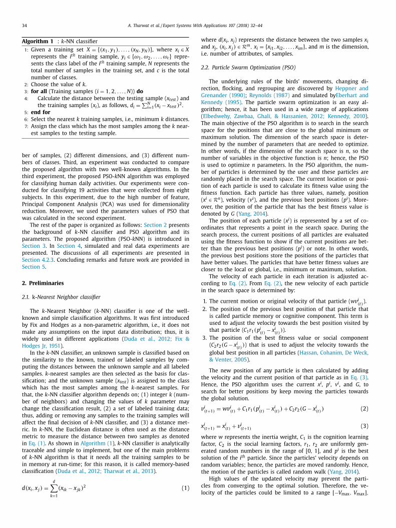
Algorithm 1 : k -NN classifier

1: Given a training set X = { (x 1 , y 1 ) , . . . , (x N , y N ) } , wher e x i ∈ X

represents the i th training sample, y i ∈ { ω 1 , ω 2 , . . . , ω c } repre-

sents the class label of the i th training sample, N represents the

total number of samples in the training set, and c is the total

number of classes.

2: Choose the value of k .

3: for all (Training samples ( i = 1 , 2 , . . . , N)) do

4: Calculate the distance between the testing sample ( x test ) and

the training samples ( x i ), as follows, d i =

∑ N i =1 (x i − x test )

2 .

5: end for

6: Select the nearest k training samples, i.e., minimum k distances.

7: Assign the class which has the most samples among the k near-

est samples to the testing sample.

w

a

i

2

r

G

K

g

(

T

s

m

m

I

n

i

b

r

t

fi

(

o

d

o

s

u

t

t

h

c

c

i

t

H

s

t

v

x

w

f

e

s

r

t

c

l

ber of samples, (2) different dimensions, and (3) different num-

bers of classes. Third, an experiment was conducted to compare

the proposed algorithm with two well-known algorithms. In the

third experiment, the proposed PSO- k NN algorithm was employed

for classifying human daily activities. Our experiments were con-

ducted for classifying 19 activities that were collected from eight

subjects. In this experiment, due to the high number of feature,

Principal Component Analysis (PCA) was used for dimensionality

reduction. Moreover, we used the parameters values of PSO that

was calculated in the second experiment.

The rest of the paper is organized as follows: Section 2 presents

the background of k -NN classifier and PSO algorithm and its

parameters. The proposed algorithm (PSO- k NN) is introduced in

Section 3 . In Section 4 , simulated and real data experiments are

presented. The discussions of all experiments are presented in

Section 4.2.3 . Concluding remarks and future work are provided in

Section 5 .

2. Preliminaries

2.1. k -Nearest Neighbor classifier

The k -Nearest Neighbor ( k -NN) classifier is one of the well-

known and simple classification algorithms. It was first introduced

by Fix and Hodges as a non-parametric algorithm, i.e., it does not

make any assumptions on the input data distribution; thus, it is

widely used in different applications ( Duda et al., 2012; Fix &

Hodges Jr, 1951 ).

In the k -NN classifier, an unknown sample is classified based on

the similarity to the known, trained or labeled samples by com-

puting the distances between the unknown sample and all labeled

samples. k -nearest samples are then selected as the basis for clas-

sification; and the unknown sample ( x test ) is assigned to the class

which has the most samples among the k -nearest samples. For

that, the k -NN classifier algorithm depends on; (1) integer k (num-

ber of neighbors) and changing the values of k parameter may

change the classification result, (2) a set of labeled training data;

thus, adding or removing any samples to the training samples will

affect the final decision of k -NN classifier, and (3) a distance met-

ric. In k -NN, the Euclidean distance is often used as the distance

metric to measure the distance between two samples as denoted

in Eq. (1) . As shown in Algorithm (1 ), k -NN classifier is analytically

traceable and simple to implement, but one of the main problems

of k -NN algorithm is that it needs all the training samples to be

in memory at run-time; for this reason, it is called memory-based

classification ( Duda et al., 2012; Tharwat et al., 2013 ).

d(x i , x j ) =

d ∑

k =1

(x ik − x jk ) 2 (1)

here d ( x i , x j ) represents the distance between the two samples x i nd x j , (x i , x j ) ∈ R

m , x i = { x i 1 , x i 2 , . . . , x im

} , and m is the dimension,

.e. number of attributes, of samples.

.2. Particle Swarm Optimization (PSO)

The underlying rules of the birds’ movements, changing di-

ection, flocking, and regrouping are discovered by Heppner and

renander (1990) ; Reynolds (1987) and simulated by Eberhart and

ennedy (1995) . The particle swarm optimization is an easy al-

orithm; hence, it has been used in a wide range of applications

Elbedwehy, Zawbaa, Ghali, & Hassanien, 2012; Kennedy, 2010 ).

he main objective of the PSO algorithm is to search in the search

pace for the positions that are close to the global minimum or

aximum solution. The dimension of the search space is deter-

ined by the number of parameters that are needed to optimize.

n other words, if the dimension of the search space is n , so the

umber of variables in the objective function is n ; hence, the PSO

s used to optimize n parameters. In the PSO algorithm, the num-

er of particles is determined by the user and these particles are

andomly placed in the search space. The current location or posi-

ion of each particle is used to calculate its fitness value using the

tness function. Each particle has three values, namely, position

x i ∈ R

n ), velocity ( v i ), and the previous best positions ( p i ). More-

ver, the position of the particle that has the best fitness value is

enoted by G ( Yang, 2014 ).

The position of each particle ( x i ) is represented by a set of co-

rdinates that represents a point in the search space. During the

earch process, the current positions of all particles are evaluated

sing the fitness function to show if the current positions are bet-

er than the previous best positions ( p i ) or note. In other words,

he previous best positions store the positions of the particles that

ave better values. The particles that have better fitness values are

loser to the local or global, i.e., minimum or maximum, solution.

The velocity of each particle in each iteration is adjusted ac-

ording to Eq. (2) . From Eq. (2) , the new velocity of each particle

n the search space is determined by:

1. The current motion or original velocity of that particle ( w v i (t)

).

2. The position of the previous best position of that particle that

is called particle memory or cognitive component. This term is

used to adjust the velocity towards the best position visited by

that particle ( C 1 r 1 (p i (t)

− x i (t)

) ).

3. The position of the best fitness value or social component

( C 2 r 2 (G − x i (t)

) ) that is used to adjust the velocity towards the

global best position in all particles ( Hassan, Cohanim, De Weck,

& Venter, 2005 ).

The new position of any particle is then calculated by adding

he velocity and the current position of that particle as in Eq. (3) .

ence, the PSO algorithm uses the current x i , p i , v i , and G , to

earch for better positions by keep moving the particles towards

he global solution.

i (t+1) = w v i (t) + C 1 r 1 (p i (t) − x i (t) ) + C 2 r 2 (G − x i (t) ) (2)

i (t+1) = x i (t) + v i (t+1) (3)

here w represents the inertia weight, C 1 is the cognition learning

actor, C 2 is the social learning factors, r 1 , r 2 are uniformly gen-

rated random numbers in the range of [0, 1], and p i is the best

olution of the i th particle. Since the particles’ velocity depends on

andom variables; hence, the particles are moved randomly. Hence,

he motion of the particles is called random walk ( Yang, 2014 ).

High values of the updated velocity may prevent the parti-

les from converging to the optimal solution. Therefore, the ve-

ocity of the particles could be limited to a range [ −V max , V max ] ,

A. Tharwat et al. / Expert Systems With Applications 107 (2018) 32–44 35

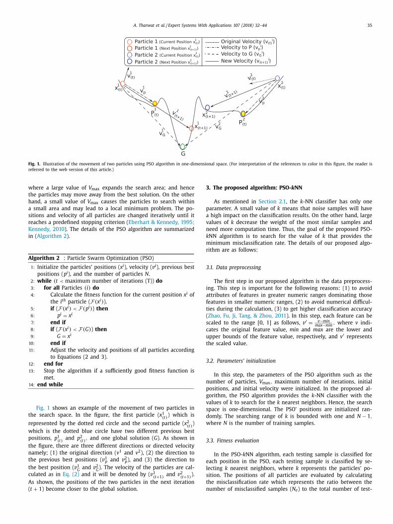
Fig. 1. Illustration of the movement of two particles using PSO algorithm in one-dimensional space. (For interpretation of the references to color in this figure, the reader is

referred to the web version of this article.)

w

t

h

a

s

r

K

i

A

t

r

w

p

t

n

t

t

c

A

(

3

p

a

v

n

k

m

r

3

i

a

f

t

(

s

c

u

t

3

n

p

g

v

s

d

w

3

e

l

s

t

n

here a large value of V max expands the search area; and hence

he particles may move away from the best solution. On the other

and, a small value of V max causes the particles to search within

small area and may lead to a local minimum problem. The po-

itions and velocity of all particles are changed iteratively until it

eaches a predefined stopping criterion ( Eberhart & Kennedy, 1995;

ennedy, 2010 ). The details of the PSO algorithm are summarized

n ( Algorithm 2 ).

lgorithm 2 : Particle Swarm Optimization (PSO)

1: Initialize the particles’ positions ( x i ), velocity ( v i ), previous best

positions ( p i ), and the number of particles N.

2: while (t < maximum number of iterations (T)) do

3: for all Particles (i ) do

4: Calculate the fitness function for the current position x i of

the i th particle ( F(x i ) ).

5: if ( F(x i ) < F(p i ) ) then

6: p i = x i

7: end if

8: if ( F(x i ) < F(G ) ) then

9: G = x i

10: end if

11: Adjust the velocity and positions of all particles according

to Equations (2 and 3).

12: end for

13: Stop the algorithm if a sufficiently good fitness function is

met.

14: end while

Fig. 1 shows an example of the movement of two particles in

he search space. In the figure, the first particle ( x 1 (t)

) which is

epresented by the dotted red circle and the second particle ( x 2 (t)

)

hich is the dotted blue circle have two different previous best

ositions, p 1 (t)

and p 2 (t)

, and one global solution ( G ). As shown in

he figure, there are three different directions or directed velocity

amely; (1) the original direction ( v 1 and v 2 ), (2) the direction to

he previous best positions ( v 1 p and v 2 p ), and (3) the direction to

he best position ( v 1 G

and v 2 G

). The velocity of the particles are cal-

ulated as in Eq. (2) and it will be denoted by ( v 1 (t+1)

and v 2 (t+1)

).

s shown, the positions of the two particles in the next iteration

t + 1 ) become closer to the global solution.

. The proposed algorithm: PSO- k NN

As mentioned in Section 2.1 , the k -NN classifier has only one

arameter. A small value of k means that noise samples will have

high impact on the classification results. On the other hand, large

alues of k decrease the weight of the most similar samples and

eed more computation time. Thus, the goal of the proposed PSO-

NN algorithm is to search for the value of k that provides the

inimum misclassification rate. The details of our proposed algo-

ithm are as follows:

.1. Data preprocessing

The first step in our proposed algorithm is the data preprocess-

ng. This step is important for the following reasons: (1) to avoid

ttributes of features in greater numeric ranges dominating those

eatures in smaller numeric ranges, (2) to avoid numerical difficul-

ies during the calculation, (3) to get higher classification accuracy

Zhao, Fu, Ji, Tang, & Zhou, 2011 ). In this step, each feature can be

caled to the range [0, 1] as follows, v ′ =

v −min max −min

, where v indi-

ates the original feature value, min and max are the lower and

pper bounds of the feature value, respectively, and v ′ represents

he scaled value.

.2. Parameters’ initialization

In this step, the parameters of the PSO algorithm such as the

umber of particles, V max , maximum number of iterations, initial

ositions, and initial velocity were initialized. In the proposed al-

orithm, the PSO algorithm provides the k -NN classifier with the

alues of k to search for the k nearest neighbors. Hence, the search

pace is one-dimensional. The PSO’ positions are initialized ran-

omly. The searching range of k is bounded with one and N − 1 ,

here N is the number of training samples.

.3. Fitness evaluation

In the PSO- k NN algorithm, each testing sample is classified for

ach position in the PSO, each testing sample is classified by se-

ecting k nearest neighbors, where k represents the particles’ po-

ition. The positions of all particles are evaluated by calculating

he misclassification rate which represents the ratio between the

umber of misclassified samples ( N e ) to the total number of test-

36 A. Tharwat et al. / Expert Systems With Applications 107 (2018) 32–44

Fig. 2. Flowchart of the proposed model PSO- k NN algorithm. (For interpretation of

the references to color in this figure, the reader is referred to the web version of

this article.)

Table 2

Description of the training data used in our simulated example.

Sample No. Class 1( ω 1 ) Class 2 ( ω 2 )

f 1 f 2 f 1 f 2

1 7 1 3 3

2 5 2 4 4

3 9 2 7 4

4 10 4 5 5

5 8 4 6 5

6 11 4 6 10

7 9 9 4 11

8 9 11 2 11

9 10 9 2 6

10 8 6 5 9

Fig. 3. Example to show how the k parameter controls the predicted class labels of

the unknown samples; hence, controls the misclassification rate.

Table 3

Description of the testing data used in our simulated example and its predicted

class labels using k -NN classifier with different values of k .

Testing samples True class label ( y i ) Predicted class labels ( ̂ y i )

Sample no. f 1 f 2 k = 1 k = 3 k = 5 k = 7 k = 9

1 7 9 1 2 2 1 1 2

2 4 2 2 1 2 2 2 2

3 9 3 1 1 1 1 1 1

4 2 7 2 2 2 2 2 2

Misclassification rate (%) 50 25 0 0 25

The bold underline values indicate the wrong class label.

4

t

m

c

F

T

i

p

f

o

i

f

ing samples ( N ) as denoted in Eq. (4) ).

Min : F =

N e

N

(4)

3.4. Termination criteria

When the termination criteria are satisfied, the iteration ends;

otherwise, we proceed with the next iteration. In the proposed

model, the PSO algorithm is terminated when a maximum num-

ber of iterations is reached.

Fig. 2 shows the overall process of the PSO- k NN algorithm. This

figure gives an example to illustrate how the predicted class de-

pends on the value of k . As shown from the figure, the training

samples consist of two classes, red circles that represent the first

class and blue stars that represent the second class. Moreover, the

testing sample is represented by a black square. In addition, the

PSO algorithm provides the k -NN classifier with k and receives the

misclassification rate. In other words, PSO- k NN iteratively changes

the value of k to minimize the misclassification rate. As shown in

Fig. 2 , the value of the k parameter controls prediction of the test-

ing samples and the misclassification rate.

Due to stochastic nature of the PSO algorithm, there is no ab-

solute guarantee for finding the optimal solution, but it iteratively

converges to a solution that is better than the random initial solu-

tion. The optimal solution changes according to the initial random

solution, the values of PSO parameters, and the random walk of

the particles.

4. Experimental results and discussion

In this section, three types of experiments were conducted. The

first experiment (see Section 4.1 ) was a simulated experiment. In

this experiment, a simulation of the proposed algorithm was run-

ning on a small number of training and testing samples to show

how the PSO- k NN algorithm converges to the best solution. In the

second experiment (see Section 4.2 ), real datasets were used to

evaluate the proposed algorithm compared with two well-known

optimization algorithms. In the third (see Section 4.3 ), experiment,

the proposed PSO- k NN algorithm was employed for recognizing

daily human activities.

.1. Simulated experiment

The aim of the optimization in this example was to search for

he k value that improves the accuracy of the k -NN classifier. As

entioned before, changing the value of k changes the predicted

lass labels; hence, changes the misclassification rate as shown in

ig. 2 . In this example, a simulated training dataset was created.

he training dataset consists of two classes, ω 1 and ω 2 , as shown

n Table 2 . As shown from the table, each class consists of ten sam-

les and each sample was represented by only two features ( f 1 and

2 ), the samples of the two classes were visualized in Fig. 3 . More-

ver, Table 3 shows the testing samples that were also visualized

n Fig. 3 . Table 3 illustrates the testing samples and the class label

or each sample.

A. Tharwat et al. / Expert Systems With Applications 107 (2018) 32–44 37

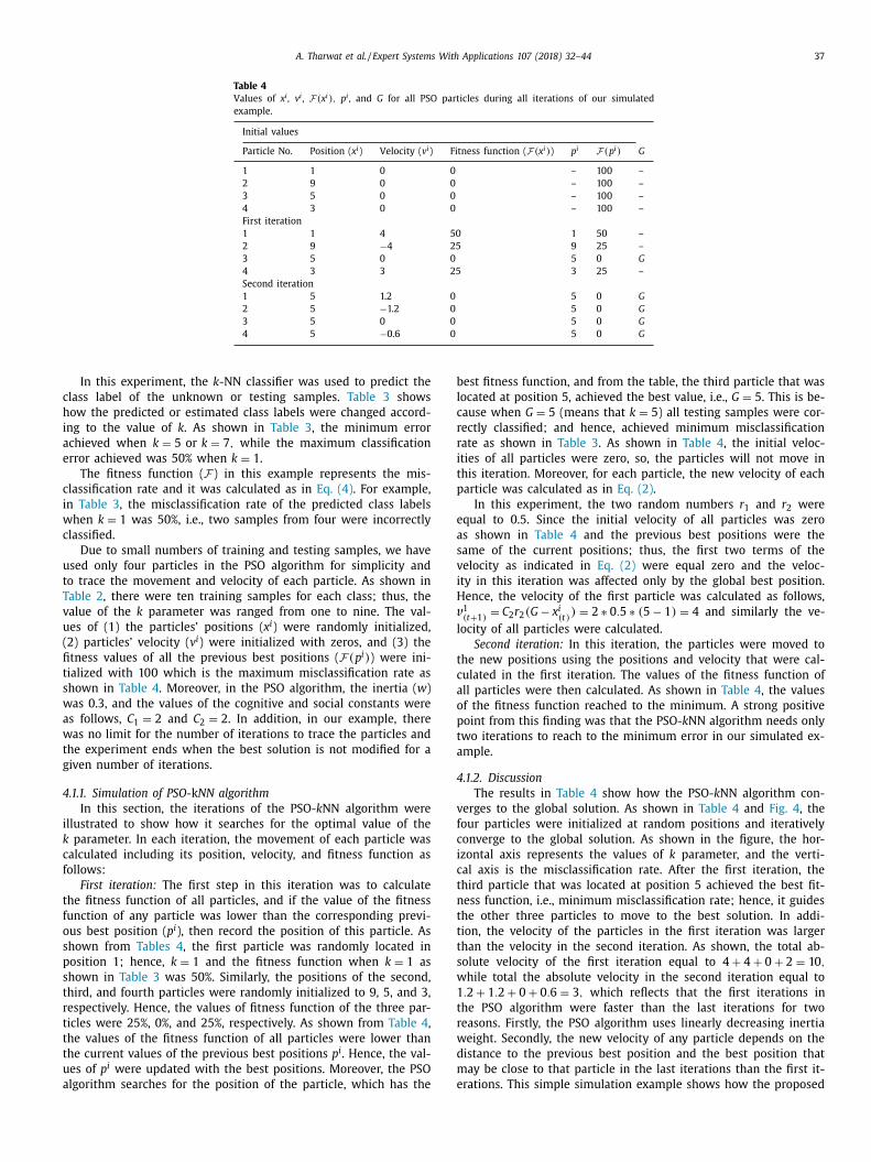
Table 4

Values of x i , v i , F(x i ) , p i , and G for all PSO particles during all iterations of our simulated

example.

Initial values

Particle No. Position ( x i ) Velocity ( v i ) Fitness function ( F(x i ) ) p i F(p i ) G

1 1 0 0 – 100 –

2 9 0 0 – 100 –

3 5 0 0 – 100 –

4 3 0 0 – 100 –

First iteration

1 1 4 50 1 50 –

2 9 −4 25 9 25 –

3 5 0 0 5 0 G

4 3 3 25 3 25 –

Second iteration

1 5 1.2 0 5 0 G

2 5 −1.2 0 5 0 G

3 5 0 0 5 0 G

4 5 −0.6 0 5 0 G

c

h

i

a

e

c

i

w

c

u

t

T

v

u

(

fi

t

s

w

a

w

t

g

4

i

k

c

f

t

f

o

s

p

s

t

r

t

t

t

u

a

b

l

c

r

r

i

t

p

e

a

s

v

i

H

v

l

t

c

a

o

p

t

a

4

v

f

c

i

c

t

n

t

t

t

s

w

1

t

r

w

d

m

e

In this experiment, the k -NN classifier was used to predict the

lass label of the unknown or testing samples. Table 3 shows

ow the predicted or estimated class labels were changed accord-

ng to the value of k . As shown in Table 3 , the minimum error

chieved when k = 5 or k = 7 , while the maximum classification

rror achieved was 50% when k = 1 .

The fitness function ( F) in this example represents the mis-

lassification rate and it was calculated as in Eq. (4) . For example,

n Table 3 , the misclassification rate of the predicted class labels

hen k = 1 was 50%, i.e., two samples from four were incorrectly

lassified.

Due to small numbers of training and testing samples, we have

sed only four particles in the PSO algorithm for simplicity and

o trace the movement and velocity of each particle. As shown in

able 2 , there were ten training samples for each class; thus, the

alue of the k parameter was ranged from one to nine. The val-

es of (1) the particles’ positions ( x i ) were randomly initialized,

2) particles’ velocity ( v i ) were initialized with zeros, and (3) the

tness values of all the previous best positions ( F(p i ) ) were ini-

ialized with 100 which is the maximum misclassification rate as

hown in Table 4 . Moreover, in the PSO algorithm, the inertia ( w )

as 0.3, and the values of the cognitive and social constants were

s follows, C 1 = 2 and C 2 = 2 . In addition, in our example, there

as no limit for the number of iterations to trace the particles and

he experiment ends when the best solution is not modified for a

iven number of iterations.

.1.1. Simulation of PSO- k NN algorithm

In this section, the iterations of the PSO- k NN algorithm were

llustrated to show how it searches for the optimal value of the

parameter. In each iteration, the movement of each particle was

alculated including its position, velocity, and fitness function as

ollows:

First iteration: The first step in this iteration was to calculate

he fitness function of all particles, and if the value of the fitness

unction of any particle was lower than the corresponding previ-

us best position ( p i ), then record the position of this particle. As

hown from Tables 4 , the first particle was randomly located in

osition 1; hence, k = 1 and the fitness function when k = 1 as

hown in Table 3 was 50%. Similarly, the positions of the second,

hird, and fourth particles were randomly initialized to 9, 5, and 3,

espectively. Hence, the values of fitness function of the three par-

icles were 25%, 0%, and 25%, respectively. As shown from Table 4 ,

he values of the fitness function of all particles were lower than

he current values of the previous best positions p i . Hence, the val-

es of p i were updated with the best positions. Moreover, the PSO

lgorithm searches for the position of the particle, which has the

est fitness function, and from the table, the third particle that was

ocated at position 5, achieved the best value, i.e., G = 5 . This is be-

ause when G = 5 (means that k = 5 ) all testing samples were cor-

ectly classified; and hence, achieved minimum misclassification

ate as shown in Table 3 . As shown in Table 4 , the initial veloc-

ties of all particles were zero, so, the particles will not move in

his iteration. Moreover, for each particle, the new velocity of each

article was calculated as in Eq. (2) .

In this experiment, the two random numbers r 1 and r 2 were

qual to 0.5. Since the initial velocity of all particles was zero

s shown in Table 4 and the previous best positions were the

ame of the current positions; thus, the first two terms of the

elocity as indicated in Eq. (2) were equal zero and the veloc-

ty in this iteration was affected only by the global best position.

ence, the velocity of the first particle was calculated as follows,

1 (t+1)

= C 2 r 2 (G − x i (t)

) = 2 ∗ 0 . 5 ∗ (5 − 1) = 4 and similarly the ve-

ocity of all particles were calculated.

Second iteration: In this iteration, the particles were moved to

he new positions using the positions and velocity that were cal-

ulated in the first iteration. The values of the fitness function of

ll particles were then calculated. As shown in Table 4 , the values

f the fitness function reached to the minimum. A strong positive

oint from this finding was that the PSO- k NN algorithm needs only

wo iterations to reach to the minimum error in our simulated ex-

mple.

.1.2. Discussion

The results in Table 4 show how the PSO- k NN algorithm con-

erges to the global solution. As shown in Table 4 and Fig. 4 , the

our particles were initialized at random positions and iteratively

onverge to the global solution. As shown in the figure, the hor-

zontal axis represents the values of k parameter, and the verti-

al axis is the misclassification rate. After the first iteration, the

hird particle that was located at position 5 achieved the best fit-

ess function, i.e., minimum misclassification rate; hence, it guides

he other three particles to move to the best solution. In addi-

ion, the velocity of the particles in the first iteration was larger

han the velocity in the second iteration. As shown, the total ab-

olute velocity of the first iteration equal to 4 + 4 + 0 + 2 = 10 ,

hile total the absolute velocity in the second iteration equal to

. 2 + 1 . 2 + 0 + 0 . 6 = 3 , which reflects that the first iterations in

he PSO algorithm were faster than the last iterations for two

easons. Firstly, the PSO algorithm uses linearly decreasing inertia

eight. Secondly, the new velocity of any particle depends on the

istance to the previous best position and the best position that

ay be close to that particle in the last iterations than the first it-

rations. This simple simulation example shows how the proposed

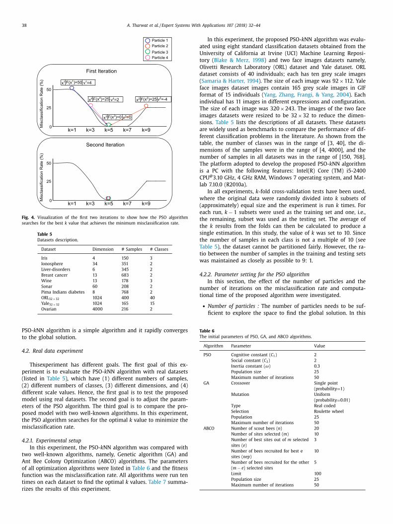
38 A. Tharwat et al. / Expert Systems With Applications 107 (2018) 32–44

Fig. 4. Visualization of the first two iterations to show how the PSO algorithm

searches for the best k value that achieves the minimum misclassification rate.

Table 5

Datasets description.

Dataset Dimension # Samples # Classes

Iris 4 150 3

Ionosphere 34 351 2

Liver-disorders 6 345 2

Breast cancer 13 683 2

Wine 13 178 3

Sonar 60 208 2

Pima Indians diabetes 8 768 2

ORL 32 × 32 1024 400 40

Yale 32 × 32 1024 165 15

Ovarian 40 0 0 216 2

a

U

t

O

d

(

f

f

i

T

i

s

a

f

t

m

n

T

i

C

l

w

(

e

t

t

s

t

T

t

w

4

n

t

Table 6

The initial parameters of PSO, GA, and ABCO algorithms.

Algorithm Parameter Value

PSO Cognitive constant ( C 1 ) 2

Social constant ( C 2 ) 2

Inertia constant ( ω) 0.3

Population size 25

Maximum number of iterations 50

GA Crossover Single point

(probability = 1)

Mutation Uniform

(probability = 0.01)

Type Real coded

Selection Roulette wheel

Population 25

Maximum number of iterations 50

ABCO Number of scout bees ( n ) 20

Number of sites selected ( m ) 10

Number of best sites out of m selected

sites ( e )

3

Number of bees recruited for best e

sites ( nep )

10

Number of bees recruited for the other

( m − e ) selected sites

5

Limit 100

Population size 25

Maximum number of iterations 50

PSO- k NN algorithm is a simple algorithm and it rapidly converges

to the global solution.

4.2. Real data experiment

Thisexperiment has different goals. The first goal of this ex-

periment is to evaluate the PSO- k NN algorithm with real datasets

(listed in Table 5 ), which have (1) different numbers of samples,

(2) different numbers of classes, (3) different dimensions, and (4)

different scale values. Hence, the first goal is to test the proposed

model using real datasets. The second goal is to adjust the param-

eters of the PSO algorithm. The third goal is to compare the pro-

posed model with two well-known algorithms. In this experiment,

the PSO algorithm searches for the optimal k value to minimize the

misclassification rate.

4.2.1. Experimental setup

In this experiment, the PSO- k NN algorithm was compared with

two well-known algorithms, namely, Genetic algorithm (GA) and

Ant Bee Colony Optimization (ABCO) algorithms. The parameters

of all optimization algorithms were listed in Table 6 and the fitness

function was the misclassification rate. All algorithms were run ten

times on each dataset to find the optimal k values. Table 7 summa-

rizes the results of this experiment.

In this experiment, the proposed PSO- k NN algorithm was evalu-

ted using eight standard classification datasets obtained from the

niversity of California at Irvine (UCI) Machine Learning Reposi-

ory ( Blake & Merz, 1998 ) and two face images datasets namely,

livetti Research Laboratory (ORL) dataset and Yale dataset. ORL

ataset consists of 40 individuals; each has ten grey scale images

Samaria & Harter, 1994 ). The size of each image was 92 × 112. Yale

ace images dataset images contain 165 grey scale images in GIF

ormat of 15 individuals ( Yang, Zhang, Frangi, & Yang, 2004 ). Each

ndividual has 11 images in different expressions and configuration.

he size of each image was 320 × 243. The images of the two face

mages datasets were resized to be 32 × 32 to reduce the dimen-

ions. Table 5 lists the descriptions of all datasets. These datasets

re widely used as benchmarks to compare the performance of dif-

erent classification problems in the literature. As shown from the

able, the number of classes was in the range of [3, 40], the di-

ensions of the samples were in the range of [4, 40 0 0], and the

umber of samples in all datasets was in the range of [150, 768].

he platform adopted to develop the proposed PSO- k NN algorithm

s a PC with the following features: Intel(R) Core (TM) i5-2400

PU

@ 3.10 GHz, 4 GHz RAM, Windows 7 operating system, and Mat-

ab 7.10.0 (R2010a).

In all experiments, k -fold cross-validation tests have been used,

here the original data were randomly divided into k subsets of

approximately) equal size and the experiment is run k times. For

ach run, k − 1 subsets were used as the training set and one, i.e.,

he remaining, subset was used as the testing set. The average of

he k results from the folds can then be calculated to produce a

ingle estimation. In this study, the value of k was set to 10. Since

he number of samples in each class is not a multiple of 10 (see

able 5 ), the dataset cannot be partitioned fairly. However, the ra-

io between the number of samples in the training and testing sets

as maintained as closely as possible to 9: 1.

.2.2. Parameter setting for the PSO algorithm

In this section, the effect of the number of particles and the

umber of iterations on the misclassification rate and computa-

ional time of the proposed algorithm were investigated.

• Number of particles : The number of particles needs to be suf-

ficient to explore the space to find the global solution. In this

A. Tharwat et al. / Expert Systems With Applications 107 (2018) 32–44 39

Table 7

The average of misclassification rate (%Mean ± SD) of ten runs of the PSO- k NN, GA- k NN, and ABCO- k NN algo-

rithms using the datasets that listed in Table 5 when the maximum number of iterations was 20.

Dataset PSO- k NN GA- k NN ABCO- k NN

Iris 1.4667 ± 0.1216 4 ± 0 2.6667 ± 0

Iono 2.1429 ± 0 4.1429 ± 0 2.9143 ± 0.5521

Liver 10.9302 ± 0.0708 11.9767 ± 0 12.4651 ± 7.4898 ×10 −15

Breast cancer 5.3021 ± 0.0037 6.0850 ± 6.4898 ×10 −15 6.2581 ± 7.4898 ×10 −15

Wine 2.0899 ± 0 2.7191 ± 3.7449 ×10 −15 2.3146 ± 0.7106

Sonar 3.45 ± 0 4.1538 ± 0 2.3077 ± 0.0271

Diabate 8.5448 ± 0.1025 8.2167 ± 3.7449 ×10 −15 9.0417 ± 7.4898 ×10 −15

ORL 32 × 32 8.5 ± 0 9.5 ± 0 8.5 ± 0

Yale 32 × 32 21.9512 ± 3.7449 ×10 −15 21.9512 ± 3.7449 ×10 −15 25.8537 ± 0.7713

Ovarian 13.0556 ± 0.0928 14.2321 ± 0.2145 13.8889 ± 0.12

Bold fonts indicate the best results.

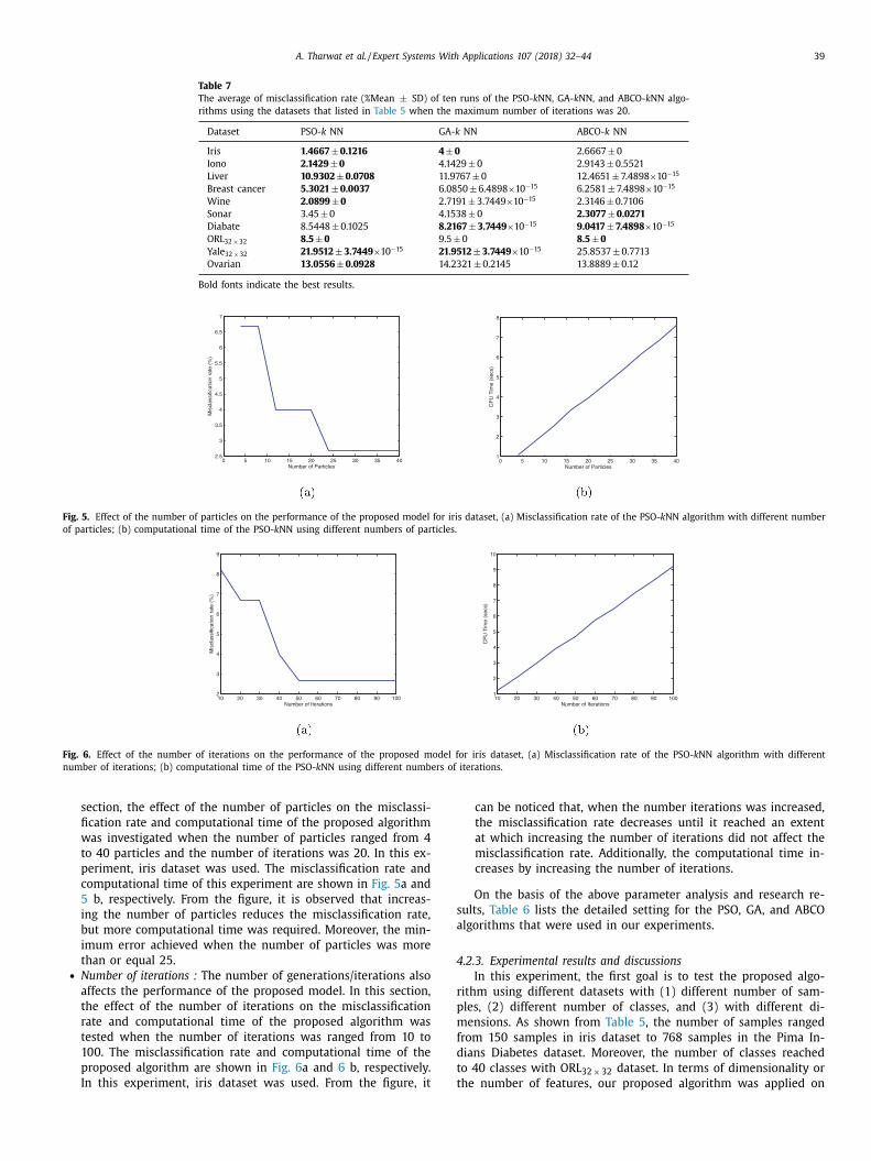
Fig. 5. Effect of the number of particles on the performance of the proposed model for iris dataset, (a) Misclassification rate of the PSO- k NN algorithm with different number

of particles; (b) computational time of the PSO- k NN using different numbers of particles.

Fig. 6. Effect of the number of iterations on the performance of the proposed model for iris dataset, (a) Misclassification rate of the PSO- k NN algorithm with different

number of iterations; (b) computational time of the PSO- k NN using different numbers of iterations.

s

a

4

r

p

m

f

d

t

t

section, the effect of the number of particles on the misclassi-

fication rate and computational time of the proposed algorithm

was investigated when the number of particles ranged from 4

to 40 particles and the number of iterations was 20. In this ex-

periment, iris dataset was used. The misclassification rate and

computational time of this experiment are shown in Fig. 5 a and

5 b, respectively. From the figure, it is observed that increas-

ing the number of particles reduces the misclassification rate,

but more computational time was required. Moreover, the min-

imum error achieved when the number of particles was more

than or equal 25. • Number of iterations : The number of generations/iterations also

affects the performance of the proposed model. In this section,

the effect of the number of iterations on the misclassification

rate and computational time of the proposed algorithm was

tested when the number of iterations was ranged from 10 to

100. The misclassification rate and computational time of the

proposed algorithm are shown in Fig. 6 a and 6 b, respectively.

In this experiment, iris dataset was used. From the figure, it

can be noticed that, when the number iterations was increased,

the misclassification rate decreases until it reached an extent

at which increasing the number of iterations did not affect the

misclassification rate. Additionally, the computational time in-

creases by increasing the number of iterations.

On the basis of the above parameter analysis and research re-

ults, Table 6 lists the detailed setting for the PSO, GA, and ABCO

lgorithms that were used in our experiments.

.2.3. Experimental results and discussions

In this experiment, the first goal is to test the proposed algo-

ithm using different datasets with (1) different number of sam-

les, (2) different number of classes, and (3) with different di-

ensions. As shown from Table 5 , the number of samples ranged

rom 150 samples in iris dataset to 768 samples in the Pima In-

ians Diabetes dataset. Moreover, the number of classes reached

o 40 classes with ORL 32 × 32 dataset. In terms of dimensionality or

he number of features, our proposed algorithm was applied on

40 A. Tharwat et al. / Expert Systems With Applications 107 (2018) 32–44

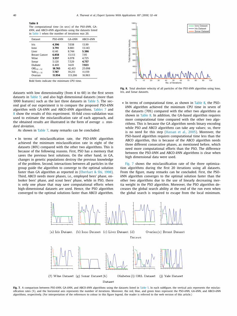
Table 8

The computational time (in secs) of the PSO- k NN, GA-

k NN, and ABCO- k NN algorithms using the datasets listed

in Table 5 when the number of iterations was 20.

Dataset PSO- k NN GA- k NN ABCO- k NN

Iris 4.396 7.038 13.99

Iono 3.791 8.881 13.143

Liver 6.141 8.744 5.386

Breast Cancer 6.858 13.113 7.95

Wine 3.557 6.978 4.725

Sonar 5.120 7.529 4.757

Diabate 8.469 14.01 7.923

ORL 32 × 32 18.765 42.413 25.098

Yale 32 × 32 7.787 19.211 11.159

Ovarian 11.954 113.266 16.963

Bold fonts indicate the minimum CPU time.

Fig. 8. Total absolute velocity of all particles of the PSO- k NN algorithm using Iono,

Iris, and Sonar datasets.

t

F

k

o

t

c

t

datasets with low dimensionality (from 4 to 60) in the first seven

datasets in Table 5 ; and also high dimensional datasets (more than

10 0 0 features) such as the last three datasets in Table 5 . The sec-

ond goal of our experiment is to compare the proposed PSO- k NN

algorithm with GA- k NN and ABCO- k NN algorithms. Tables 7 and

8 show the results of this experiment. 10-fold cross-validation was

used to estimate the misclassification rate of each approach, and

the obtained results are illustrated in the form of average ± stan-

dard deviation .

As shown in Table 7 , many remarks can be concluded:

• In terms of misclassification rate, the PSO- k NN algorithm

achieved the minimum misclassification rate in eight of the

datasets (80%) compared with the other two algorithms. This is

because of the following reasons. First, PSO has a memory that

saves the previous best solutions. On the other hand, in GA,

changes in genetic populations destroy the previous knowledge

of the problem. Second, interactions between all particles in the

group guide the algorithm to converge to the optimal solution

faster than GA algorithm as reported in ( Eberhart & Shi, 1998 ).

Third, ABCO needs more phases, i.e., employed bees’ phase, on-

looker bees’ phase, and scout bees’ phase, while in PSO, there

is only one phase that may save computational efforts when

high-dimensional datasets are used. Hence, the PSO algorithm

converged to the optimal solutions faster than ABCO algorithm.

Fig. 7. A comparison between PSO- k NN, GA- k NN, and ABCO- k NN algorithms using the da

sification rates (%), and the horizontal axis represents the number of iterations. Moreov

algorithms, respectively. (For interpretation of the references to colour in this figure legen

• In terms of computational time, as shown in Table 8 , the PSO-

k NN algorithm achieved the minimum CPU time in seven of

the datasets (70%) compared with the other two algorithms as

shown in Table 8 . In addition, the GA-based algorithm requires

more computational time compared with the other two algo-

rithms. This is because the GA algorithm needs binary encoding

while PSO and ABCO algorithms can take any values; so, there

is no need for this step ( Hassan et al., 2005 ). Moreover, the

PSO-based algorithm requires computational time less than the

ABCO algorithm, this is because of the ABCO algorithm needs

three different consecutive phases, as mentioned before, which

need more computational efforts than the PSO. The difference

between the PSO- k NN and ABCO- k NN algorithms is clear when

high dimensional data were used.

Fig. 7 shows the misclassification rate of the three optimiza-

ion algorithms during the first 20 iterations using all datasets.

rom the figure, many remarks can be concluded. First, the PSO-

NN algorithm converges to the optimal solution faster than the

ther two algorithms due to the use of linearly decreasing iner-

ia weight in the PSO algorithm. Moreover, the PSO algorithm de-

reases the global search ability at the end of the run even when

he global search is required to escape from the local minimum.

tasets listed in Table 5 . In each subfigure, the vertical axis represents the misclas-

er, the red, blue, and green lines represent the PSO- k NN, GA- k NN, and ABCO- k NN

d, the reader is referred to the web version of this article.)

A. Tharwat et al. / Expert Systems With Applications 107 (2018) 32–44 41

Fig. 9. Visualization of the positions of all particles of the PSO- k NN algorithm and misclassified samples after the first and tenth iterations. (For interpretation of the

references to color in this figure, the reader is referred to the web version of this article.)

T

b

r

F

o

s

t

f

c

s

S

G

t

b

s

c

w

d

t

F

s

c

w

i

n

m

m

p

t

p

a

c

P

G

p

M

c

p

k

i

f

t

c

4

i

a

c

4

m

I

T

hus, the PSO algorithm converges quickly at the first iterations,

ut it is slow when it becomes near to the optimal solution as

eported in ( Shi & Eberhart, 1999 ). This finding is consistent with

ig. 8 . This figure shows the total absolute velocity of all particles

f the PSO algorithm during the first 100 iterations using iris, iono-

phere, and sonar datasets. As shown, the velocity of the first itera-

ions was at maximum, which reflects that how the particles were

ast in the first iterations. On the other hand, the velocity dramati-

ally decreased, because the particles became closer to the optimal

olution than before (as mentioned in our simulated example in

ection 4.1 ). Second, the PSO- k NN algorithm was more stable than

A- k NN and ABCO- k NN algorithms.

A simple experiment was conducted to show how the posi-

ions of the particles of the PSO algorithm were converged to the

est solution(s). In this experiment, iris dataset was used. Fig. 9

hows the results of this experiment. In this experiment, the Prin-

ipal Component Analysis (PCA) technique ( Tharwat, 2016; Thar-

at, Gaber, Ibrahim, & Hassanien, 2017 ) was used to reduce the

imensions of all samples to only two attributes to visualize all

raining and testing samples in a two-dimensional space as in

ig. 9 b and 9 d. As shown in the figure, the training samples were

cattered in black, the testing samples were colored, and the mis-

lassified samples after the first and tenth iterations were marked

ith a red circle. As shown in Fig. 9 a, the value of k after the first

teration was ranged from 3 to 40, and the minimum value of fit-

ess function achieved when k = 3 or k = 13 . Fig. 9 b shows two

isclassified samples when the value of k = 3 , hence the mini-

um misclassification rate was 2.667%. As shown in Fig. 9 c, all

articles were converged to the best solution where k = 1 after the

6

enth iteration. Using k = 1 there was only one misclassified sam-

le as shown in Fig. 9 and the error rate decreased to 1.334%.

To sum up, the developed PSO- k NN algorithm yielded more

ppropriate values for the k parameter and hence obtained low

lassification error rates across different datasets. Moreover, the

SO- k NN algorithm obtained competitive results compared with

A- k NN and ABCO- k NN algorithms. Further, PSO- k NN achieved

romising results when the high dimensional data were used.

oreover, the PSO- k NN obtained competitive results in a short

omputational time when the datasets with a high number of sam-

les were used. Even so, we still cannot guarantee that the PSO-

NN algorithm must perform well and outperform other methods

n different applications. In fact, many factors may have an ef-

ect on the quality of the proposed model such as the representa-

iveness, diversity of training sets, the number of samples in each

lass, and the number of features.

.3. Human activities recognition experiments

The aim of this experiment is to classify human activities us-

ng the proposed PSO- k NN algorithm. In this experiment, the PSO

lgorithm searches for the optimal k value to minimize the mis-

lassification rate as in the second experiment.

.3.1. Experimental setup

The settings of this experiment were as in the second experi-

ent. The data was obtained from the University of California at

rvine (UCI) Machine Learning Repository ( Blake & Merz, 1998 ).

he data were collected from eight subjects; each subject has

0 samples that were sensed from 19 activities. Hence, each

42 A. Tharwat et al. / Expert Systems With Applications 107 (2018) 32–44

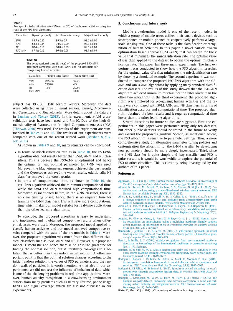
Table 9

Average of misclassification rate (%Mean ± SD) of the human activities using ten

runs of the PSO- k NN algorithm.

Classifiers Gyroscopes only Accelerometers only Magnetometers only

SVM 84.7 ± 0.17 95.3 ± 0.7 98.6 ± 0.06

ANN 84.3 ± 0.14 94.6 ± 0.09 98.8 ± 0.04

NB 67.4 ± 0.15 80.8 ± 0.09 89.5 ± 0.08

PSO- k NN 87.8 ± 0.12 96.4 ± 0.08 98.7 ± 0.03

Table 10

The computational time (in secs) of the proposed PSO- k NN

algorithm compared with SVM, ANN, and NB classifiers for

recognizing human activities.

Classifiers Training time (secs) Testing time (secs)

SVM 2356.97 35.53

ANN 2416.0 4.5

NB 1.66 20.44

PSO- k NN – 10.84

5

w

s

s

n

o

v

o

fi

p

f

b

d

k

c

a

o

r

s

c

r

l

p

b

a

t

c

c

n

t

q

P

a

R

A

A

A

A

B

B

B

B

B

B

subject has 19 × 60 = 1140 feature vectors. Moreover, the data

were collected using three different sensors, namely, Accelerome-

ter, Gyroscopes , and Magnetometer . More details about the data are

in Barshan and Yüksek (2013) . In this experiment, k -fold cross-

validation tests have been used, and k = 10 . Due to the high di-

mensionality of features, the Principal Component Analysis (PCA)

( Tharwat, 2016 ) was used. The results of this experiment are sum-

marized in Tables 9 and 10 . The results of our experiments were

compared with one of the recent related work ( Barshan & Yük-

sek, 2013 ).

As shown in Tables 9 and 10 , many remarks can be concluded:

• In terms of misclassification rate as in Table 10 , the PSO- k NN

algorithm obtained results better than SVM, ANN, and NB clas-

sifiers. This is because the PSO- k NN is optimized and hence

the optimal or near optimal parameter for k -NN was used.

Moreover, the Magnetometers sensors achieved the best results

and the Gyroscopes achieved the worst results. Additionally, NB

classifier achieved the worst results. • In terms of computational time, as shown in Table 10 , the

PSO- k NN algorithm achieved the minimum computational time,

while the SVM and ANN required high computational time.

Moreover, as mentioned before, in the k -NN classifier, there is

no clear training phase; hence, there is no required time for

training the k -NN classifiers. This will save more computational

time which makes our model suitable for real-time applications

than the other learning algorithms.

To conclude, the proposed algorithm is easy to understand

and implement and it obtained competitive results when differ-

ent datasets were used. Moreover, the proposed model applied to

classify human activities and our model achieved competitive re-

sults compared with the state-of-the-art models in Table 1 . More-

over, the proposed algorithm was much faster than different clas-

sical classifiers such as SVM, ANN, and NB. However, our proposed

model is stochastic and hence there is no absolute guarantee for

finding the optimal solution, but it iteratively converges to a so-

lution that is better than the random initial solution. Another im-

portant point is that the optimal solution changes according to the

initial random solution, the values of PSO parameters, and the ran-

dom walk of particles. It is worth mentioning that also in our ex-

periments; we did not test the influence of imbalanced data which

is one of the challenging problems in real-time applications. More-

over, human activity recognition in a crowdsensing environment

suffers from many problems such as battery lifetime, phone usage

habits, and signal coverage, which are also not discussed in our

experiments.

. Conclusions and future work

Mobile crowdsensing model is one of the recent models in

hich a group of mobile users utilizes their smart devices such as

martphones or mobile phones to cooperatively perform a large-

cale sensing task. One of these tasks is the classification or recog-

ition of human activities. In this paper, a novel particle swarm

ptimization based approach (PSO- k NN) that can search for the k

alue that minimizes the misclassification rate. The optimal value

f k is then applied to the dataset to obtain the optimal misclassi-

cation rate. This paper has three main experiments. The first ex-

eriment was conducted to show how the PSO algorithm searches

or the optimal value of k that minimizes the misclassification rate

y showing a simulated example. The second experiment was con-

ucted to compare the proposed PSO- k NN algorithm with the GA-

NN and ABCO- k NN algorithms by applying many standard classifi-

ation datasets. The results of this study showed that the PSO- k NN

lgorithm achieved minimum misclassification rates lower than the

ther two algorithms. In the third experiment, the proposed algo-

ithm was employed for recognizing human activities and the re-

ults were compared with SVM, ANN, and NB classifiers in terms of

lassification accuracy and computational time. The proposed algo-

ithm obtained the best results and it requires computational time

ower than the other learning algorithms.

Several directions for future studies are suggested. First, the ex-

eriments in this paper were performed using only ten datasets,

ut other public datasets should be tested in the future to verify

nd extend the proposed algorithm. Second, as mentioned before,

he PSO algorithm is sensitive to parameter settings. Thus, a more

omprehensive study on alternative parameter tuning policies and

ustomization the algorithm for the k -NN classifier by developing

ew parameters should be more deeply investigated. Third, since

he k -NN classifier is quite simple and lazy classifier and PSO is

uite versatile, it would be worthwhile to explore the potential of

SO to other classifiers. This is currently being investigated by the

uthors of this paper.

eferences

ggarwal, J. K. , & Cai, Q. (1997). Human motion analysis: A review. In Proceedings of

the IEEE nonrigid and articulated motion workshop (pp. 90–102). IEEE . hmed, N. , Rutten, M. , Bessell, T. , Kanhere, S. S. , Gordon, N. , & Jha, S. (2010). De-

tection and tracking using particle-filter-based wireless sensor networks. IEEETransactions on Mobile Computing, 9 (9), 1332–1345 .

Allen, F. R. , Ambikairajah, E. , Lovell, N. H. , & Celler, B. G. (2006). Classification ofa known sequence of motions and postures from accelerometry data using

adapted Gaussian mixture models. Physiological Measurement, 27 (10), 935 .

minian, K. , Robert, P. , Buchser, E. , Rutschmann, B. , Hayoz, D. , & Depairon, M. (1999).Physical activity monitoring based on accelerometry: Validation and compari-

son with video observation. Medical & Biological Engineering & Computing, 37 (3),304–308 .

nguita, D. , Ghio, A. , Oneto, L. , Parra, X. , & Reyes-Ortiz, J. L. (2012). Human activ-ity recognition on smartphones using a multiclass hardware-friendly support

vector machine. In Proceedings of the international workshop on ambient assisted

living (pp. 216–223). Springer . andouch, J. , Jenkins, O. C. , & Beetz, M. (2012). A self-training approach for visual

tracking and recognition of complex human activity patterns. International Jour-nal of Computer Vision, 99 (2), 166–189 .

Bao, L. , & Intille, S. S. (2004). Activity recognition from user-annotated accelera-tion data. In Proceedings of the international conference on pervasive computing

(pp. 1–17). Springer .

arshan, B. , & Yüksek, M. C. (2013). Recognizing daily and sports activities in twoopen source machine learning environments using body-worn sensor units. The

Computer Journal, 57 (11), 1649–1667 . edogni, L. , Bononi, L. , Di Felice, M. , D’Elia, A. , Mock, R. , Morandi, F. , et al. (2016).

An integrated simulation framework to model electric vehicle operations andservices. IEEE Transactions on Vehicular Technology, 65 (8), 5900–5917 .

edogni, L. , Di Felice, M. , & Bononi, L. (2012). By train or by car? detecting the user’smotion type through smartphone sensors data. In Wireless days (wd), 2012 IFIP

(pp. 1–6). IEEE .

edogni, L. , Gramaglia, M. , Vesco, A. , Fiore, M. , Härri, J. , & Ferrero, F. (2015). TheBologna ringway dataset: Improving road network conversion in sumo and val-

idating urban mobility via navigation services. IEEE Transactions on VehicularTechnology, 64 (12), 5464–5476 .

lake, C., Merz, C. J. (1998). UCI repository of machine learning databases.

A. Tharwat et al. / Expert Systems With Applications 107 (2018) 32–44 43

C

D

D

E

E

E

E

E

E

E

E

F

G

G

H

H

I

I

K

K

L

L

L

L

L

L

M

M

M

M

P

R

R

S

S

S

S

S

S

T

T

T

T

T

T

T

V

W

Y

Y

Y

YY

Z

arbajo, R. S. , Carbajo, E. S. , Basu, B. , & Mc Goldrick, C. (2017). Routing in wirelesssensor networks for wind turbine monitoring. Pervasive and Mobile Computing,

39 , 1–35 . arby, J. , Li, B. , & Costen, N. (2010). Tracking human pose with multiple activity

models. Pattern Recognition, 43 (9), 3042–3058 . uda, R. O. , Hart, P. E. , & Stork, D. G. (2012). Pattern classification . John Wiley & Sons .

berhart, R. C. , & Kennedy, J. (1995). A new optimizer using particle swarm theory.In Proceedings of the sixth international symposium on micro machine and human

science: 1 (pp. 39–43). New York, NY .

berhart, R. C. , & Shi, Y. (1998). Comparison between genetic algorithms and particleswarm optimization. In Evolutionary programming vii (pp. 611–616). Springer .

lbedwehy, M. N. , Zawbaa, H. M. , Ghali, N. , & Hassanien, A. E. (2012). Detection ofheart disease using binary particle swarm optimization. In Proceedings of the

federated conference on computer science and information systems (fedcsis), Wroc,Poland, September 9–12 (pp. 177–182). IEEE .

lhoseny, M. , Elminir, H. , Riad, A. , & Yuan, X. (2014). Recent advances of secure clus-

tering protocols in wireless sensor networks. International Journal of ComputerNetworks and Communications Security, 2 (11), 400–413 .

lhoseny, M. , Farouk, A. , Zhou, N. , Wang, M.-M. , Abdalla, S. , & Batle, J. (2017). Dy-namic multi-hop clustering in a wireless sensor network: Performance improve-

ment. Wireless Personal Communications, 95 (4), 3733–3753 . lhoseny, M. , Tharwat, A . , Farouk, A . , & Hassanien, A . E. (2017). K-Coverage model

based on genetic algorithm to extend WSN lifetime. IEEE Sensors Letters, 1 (4),

1–4 . lhoseny, M. , Tharwat, A. , Yuan, X. , & Hassanien, A. E. (2018). Optimizing k-coverage

of mobile WSNs. Expert Systems with Applications, 92 , 142–153 . lhoseny, M. , Yuan, X. , Yu, Z. , Mao, C. , El-Minir, H. K. , & Riad, A. M. (2015). Balancing

energy consumption in heterogeneous wireless sensor networks using geneticalgorithm. IEEE Communications Letters, 19 (12), 2194–2197 .

ix, E. , & Hodges Jr, J. L. (1951). Discriminatory analysis-nonparametric discrimina-

tion: consistency properties. Technical Report DTIC Document . DTIC . aing, Z.-L. (2004). A particle swarm optimization approach for optimum design

of pid controller in AVR system. IEEE Transactions on Energy Conversion, 19 (2),384–391 .

hosh, A. K. (2006). On optimum choice of k in nearest neighbor classification.Computational Statistics & Data Analysis, 50 (11), 3113–3123 .

assan, R. , Cohanim, B. , De Weck, O. , & Venter, G. (2005). A comparison of particle

swarm optimization and the genetic algorithm. In Proceedings of the 1st AIAAmultidisciplinary design optimization specialist conference, Honolulu, Hawaii, April

23–26 (pp. 1–13) . eppner, F. , & Grenander, U. (1990). A stochastic nonlinear model for coordinated bird

flocks. . American Association For the Adavancement of Science, Washington, DC(USA) .

brahim, A ., Tharwat, A ., Gaber, T., & Hassanien, A. E. (2017). Optimized superpixel

and adaboost classifier for human thermal face recognition. Signal, Image andVideo Processing , 1–9 in press. doi: 10.1007/s11760-017-1212-6 .

slam, M. J. , Wu, Q. J. , Ahmadi, M. , & Sid-Ahmed, M. A. (2007). Investigatingthe performance of Naive-Bayes classifiers and k-nearest neighbor classifiers.

In Proceedings of international conference on convergence information technology(pp. 1541–1546). IEEE .

ao, C.-C. , Chuang, C.-W. , & Fung, R.-F. (2006). The self-tuning pid control in a slid-er–crank mechanism system by applying particle swarm optimization approach.

Mechatronics, 16 (8), 513–522 .

ennedy, J. (2010). Particle swarm optimization. In Encyclopedia of machine learning(pp. 760–766). Springer .

achenbruch, P. A. , & Mickey, M. R. (1968). Estimation of error rates in discriminantanalysis. Technometrics, 10 (1), 1–11 .

akany, H. (2008). Extracting a diagnostic gait signature. Pattern Recognition, 41 (5),1627–1637 .

in, S.-W. , Ying, K.-C. , Chen, S.-C. , & Lee, Z.-J. (2008). Particle swarm optimization

for parameter determination and feature selection of support vector machines.Expert Systems with Applications, 35 (4), 1817–1824 .

iu, Y. , Wang, G. , Chen, H. , Dong, H. , Zhu, X. , & Wang, S. (2011). An improved parti-cle swarm optimization for feature selection. Journal of Bionic Engineering, 8 (2),

191–200 . uštrek, M. , & Kaluža, B. (2009). Fall detection and activity recognition with machine

learning. Informatica, 33 (2) .

uts, J. , Ojeda, F. , Van de Plas, R. , De Moor, B. , Van Huffel, S. , & Suykens, J. A. (2010).A tutorial on support vector machine-based methods for classification problems

in chemometrics. Analytica Chimica Acta, 665 (2), 129–145 . antyjarvi, J. , Himberg, J. , & Seppanen, T. (2001). Recognizing human motion with

multiple acceleration sensors. In IEEE international conference on systems, man,and cybernetics: 2 (pp. 747–752). IEEE .

irjalili, S. (2015a). The ant lion optimizer. Advances in Engineering Software, 83 ,

80–98 .

irjalili, S. (2015b). How effective is the grey wolf optimizer in training multi-layerperceptrons. Applied Intelligence, 43 (1), 150–161 .

ontori, F. , Bedogni, L. , Di Chiappari, A. , & Bononi, L. (2016). Sensquare: A mobilecrowdsensing architecture for smart cities. In Proceedings of the IEEE third world

forum on internet of things (wf-iot) (pp. 536–541). IEEE . reece, S. J. , Goulermas, J. Y. , Kenney, L. P. , Howard, D. , Meijer, K. , & Cromp-

ton, R. (2009). Activity identification using body-mounted sensorsa review ofclassification techniques. Physiological Measurement, 30 (4), R1 .

einhardt, A. , Christin, D. , & Kanhere, S. S. (2013). Predicting the power consumption

of electric appliances through time series pattern matching. In Proceedings of thefifth ACM workshop on embedded systems for energy-efficient buildings (pp. 1–2).

ACM . eynolds, C. W. (1987). Flocks, herds and schools: A distributed behavioral model.

ACM Siggraph Computer Graphics, 21 (4), 25–34 . amaria, F. S. , & Harter, A. C. (1994). Parameterisation of a stochastic model for hu-

man face identification. In Proceedings of the second IEEE workshop on applica-

tions of computer vision (pp. 138–142). IEEE . hi, Y. , & Eberhart, R. C. (1999). Empirical study of particle swarm optimization. In

Proceedings of the 1999 congress on evolutionary computation, (cec), Washington,DC, USA, July 6–9: 3 . IEEE .

ingh, G. , Bansal, D. , Sofat, S. , & Aggarwal, N. (2017). Smart patrolling: An efficientroad surface monitoring using smartphone sensors and crowdsourcing. Pervasive

and Mobile Computing, 40 .

ong, K.-T. , & Wang, Y.-Q. (2005). Remote activity monitoring of the elderly using atwo-axis accelerometer. In Proceedings of the CACS automatic control conference

(pp. 18–19) . tone, M. (1978). Cross-validation: A review 2. Statistics: A Journal of Theoretical and

Applied Statistics, 9 (1), 127–139 . ubasi, A. (2013). Classification of emg signals using pso optimized svm for di-

agnosis of neuromuscular disorders. Computers in Biology and Medicine, 43 (5),

576–586 . harwat, A. (2016). Principal component analysis-a tutorial. International Journal of

Applied Pattern Recognition, 3 (3), 197–240 . harwat, A. , Gaber, T. , Ibrahim, A. , & Hassanien, A. E. (2017). Linear discriminant

analysis: A detailed tutorial. AI Communications, 30 (2), 169–190 . harwat, A. , Ghanem, A. M. , & Hassanien, A. E. (2013). Three different classifiers for

facial age estimation based on k-nearest neighbor. In Proceedings of nin th IEEE

international computer engineering conference (ICENCO), Giza, Egypt, Dec. 28–29(pp. 55–60) .

harwat, A., & Hassanien, A. E. (2017). Chaotic antlion algorithm for parameteroptimization of support vector machine. Applied Intelligence , 1–17 in press.

doi: 10.1007/s10489- 017- 0994- 0 . harwat, A. , Hassanien, A. E. , & Elnaghi, B. E. (2016). A ba-based algorithm for pa-

rameter optimization of support vector machine. Pattern Recognition Letters, 93 ,

13–22 . itterton, D. , & Weston, J. L. (2004). Strapdown inertial navigation technology : 17. IET .

omasini, M. , Mahmood, B. , Zambonelli, F. , Brayner, A. , & Menezes, R. (2017). On theeffect of human mobility to the design of metropolitan mobile opportunistic

networks of sensors. Pervasive and Mobile Computing, 38 , 215–232 . esterstrøm, J. , & Thomsen, R. (2004). A comparative study of differential evolution,

particle swarm optimization, and evolutionary algorithms on numerical bench-mark problems. In Proceedings of congress on volutionary computation, CEC2004,

Alabama, USA, June 19–23: 2 (pp. 1980–1987). IEEE .

ang, X. , Yang, J. , Teng, X. , Xia, W. , & Jensen, R. (2007). Feature selection based onrough sets and particle swarm optimization. Pattern Recognition Letters, 28 (4),

459–471 . amany, W. , Fawzy, M. , Tharwat, A . , & Hassanien, A . E. (2015a). Moth-flame op-

timization for training multi-layer perceptrons. In Proceedings of the eleventhinternational conference on computer engineering (ICENCO), 2015 (pp. 267–272).

IEEE .

amany, W. , Tharwat, A. , Hassanin, M. F. , Gaber, T. , Hassanien, A. E. , &Kim, T.-H. (2015b). A new multi-layer perceptrons trainer based on ant lion

optimization algorithm. In Proceedings of the fourth international conference oninformation science and industrial applications (ISI), (pp. 40–45). IEEE .

ang, J. , Zhang, D. , Frangi, A. F. , & Yang, J.-y. (2004). Two-dimensional PCA: A newapproach to appearance-based face representation and recognition. IEEE Trans-

actions on Pattern Analysis and Machine Intelligence, 26 (1), 131–137 .

ang, X.-S. (2014). Nature-inspired optimization algorithms (1st ed). Elsevier . ao, J. , Kanhere, S. S. , & Hassan, M. (2008). An empirical study of bandwidth pre-

dictability in mobile computing. In Proceedings of the third ACM internationalworkshop on wireless network testbeds, experimental evaluation and characteriza-

tion (pp. 11–18). ACM . hao, M. , Fu, C. , Ji, L. , Tang, K. , & Zhou, M. (2011). Feature selection and parameter

optimization for support vector machines: A new approach based on genetic

algorithm with feature chromosomes. Expert Systems with Applications, 38 (5),5197–5204 .

44 A. Tharwat et al. / Expert Systems With Applications 107 (2018) 32–44

niversity, M.Sc. in 2008 Mansoura University, and Ph.D. in 2017 from Suez Canal Univer-

the framework of the Welcome project - Erasmus Mundus Action 2 - with a title ‘Novel ion‘ in 2015. Currently, he is a researcher in Faculty of Computer Science and Engineer-

m Main, Germany. He is an author of many research studies published at national and

research interests include pattern recognition, machine learning, digital image processing,

rded in 2015 the Distinguished University Award of Ain Shams University, Cairo, Egypt.

nd Systems Engineering Department, Faculty of Engineering, Ain Shams University, Cairo, ot his M.Sc. in Electrical Engineering in 1976. He got his Doctor from Technische Univer-

st-Doctoral Research Fellow at the Electrical and Computer Engineering Department, The and at the Computer Vision and Image Processing (CVIP) Lab, Electrical Engineering De-

He was on a leave of absence to work with Al-Isra University (Amman, Jordan), El-Emarat

Collage (Hufuf, Saudi Arabia).

r and Information from Mansoura University, Egypt (in a scientific research channel with

ity of North Texas, USA). Dr. Elhoseny is currently an Assistant Professor at the Faculty of vely, Dr. Elhoseny authored/co-authored over 70 International Journal articles, Conference

search interests include Network Security, Cryptography, Machine Learning Techniques, y serves as the Editor-in-Chief of Big Data and Cloud Innovation Journal and Associate

e journal. Dr. Elhoseny guest-edited several special issues at many journals published by r, he served as the co-chair, the publication chair, the program chair, and a track chair for

pringer.

986 and M.Sc. degree in 1993, both from Ain Shams University, Faculty of Science, Pure ypt. On September 1998, he received his doctoral degree from the Department of Com-

okyo Institute of Technology, Japan. He is the Founder and Head of the Egyptian Scientific

nology at the Faculty of Computer and Information, Cairo University. He has more than ternational journals and he has more than 30 books in the topics of data mining and

works and smart environment.

Alaa Tharwat received his B.Sc. in 2002 from Mansoura U

sity. He worked as a researcher at Gent University, withinapproach of multi-modal biometrics for animal identificat

ing, Frankfurt University of Applied Sciences, Frankfurt a

international journals, conference proceedings. His major biometric authentication, and bio-inspired optimization.

Hani Mahdi is an IEEE Life Senior Member. He was awa

Hani Mahdi is a Computer Systems Professor, Computer aEgypt. From this university he is graduated in 1971 and g

sitaet, Braunschweig, West Germany, in 1984. He was a PoPennsylvania State University, Pennsylvania (1988–1989),

partment, University of Louisville, Kentucky (20 01–20 02).

University (El Ain,United Arab Emirates), and Technology

Mohamed Elhoseny received the Ph.D. degree in Compute

Department of Computer Science and Engineering, UniversComputers and Information, Mansoura University. Collecti

Proceedings, Book Chapters, and 3 Springer books. His reInternet of Things, and Quantum Computing. Dr. Elhosen

Editor of many journals such as IEEE Access, and PLOS OnIEEE, Hindawi, Springer, Inderscience, and MDPI. Moreove

several international conferences published by IEEE and S

Aboul Ella Hassanien received his B.Sc. with honors in 1Mathematics and Computer Science Department, Cairo, Eg

puter Science, Graduate School of Science & Engineering, T

Research Group (SRGE) and Professor of Information Tech500 scientific research papers published in prestigious in

medical images and intelligent systems address social net