experimental technique to investigate … · result.the objective of the paper is using modal...

EXPERIMENTAL TECHNIQUE TO INVESTIGATE VIBRATION

MONITORING IN REVOLVING STRUCTURES USING OSCILLOSCOPIC

/MODAL TESTING

H.A.H.AL-KHAZALI1 1 School of Mechanical & Automotive Engineering, Kingston University, London, UK

E-mail, [email protected]

M.R.ASKARI2 2 School of Aerospace & Aircraft Engineering, Kingston University, London, UK

E-mail, [email protected]

Abstract: Linear structures for the purpose of vibration analysis may be modelled either as a continuous system or a discrete one.In the case of the latter method the mass of the system is lumped into a finite number of masses connected by springs and dampers representing the stiffness and damping in the system respectively. The system is then said to possess an finite number of degrees of freedom.In this paper search of finding a new technique for interpret the results obtained from experiment measurement of dynamic performance of machinery for condition monitoring,it is envisage that a database could be created. This database consisting of complete mathematical model of the machine which includes both the supporting structures as well as the moving parts and is based on the structural dynamics characteristics of the system. The experimental technique used thus far is called Modal Testing, a well known and widely used technique in research and industry to obtain the modal and Dynamic response properties of structures.The technique has recently been applied to rotating structures and some research papers been published, however the full implementation of Modal Testing in active structures and the implications are not fully understood and are therefore in need of much further and more in depth investigations. The raw data obtained from experiment was used in Simulation finite element (FE) model (ANSYS 12) for comparison,it has good capability for Eigen analysis and also good graphical facility and obtained good result.The objective of the paper is using modal testing and analysis results for structural health monitoring purpose. Keywords: Oscilloscopic technique;Experimental /Computational techniques;Vibration monitoring;Rotor dynamic;Modal testing. 1. Introduction

The equations of motion of the discrete model consists of a finite number of second order ordinary differential equations coupled together, in which case they have to be solved simultaneously[1,2].The process becomes progressively more difficult as the number of degrees of freedom increases.In modal testing, FRF measurements are usually made under controlled conditions, where the test structure is artificially excited by using either an impact hammer, or one or more shakers driven by broadband signals. A multi-channel FFT analyzer is then used to make FRF measurements between input and output DOF pairs on the test structure.Modal testing requires that FRFs be measured from at least one row or column of the FRF matrix.Modal frequency & damping are global properties of a structure, and can be estimated from any or all of the FRFs in a row or column of the FRF matrix. On the other hand, each mode shape is obtained by assembling together FRF numerator terms (called residues) from at least one row or column of the FRF matrix [3,4].Not all structures can be impact tested, however. For instance, structure with delicate surfaces cannot be impact tested, or because of its limited frequency range or low energy density over a wide spectrum, the impacting force is not be sufficient to

H.A.H.Al-Khazali et al. / International Journal of Engineering Science and Technology (IJEST)

ISSN : 0975-5462 Vol. 3 No.10 October 2011 7799

adequately excite the modes of interest. When impact testing cannot be used, FRF measurements must be made by providing artificial excitation with one or more shakers, attached to the structure [3,5]. There is a way of de-coupling the equations of motion using the orthogonality properties of the natural modes. In this method,the system is transformed from generalised coordinates to a new set of coordinates called principal coordinates, in which case the equations are solved independently and inverse transformed into the generalised coordinates. The method of de-coupling the equations of motion is called Modal analysis [1,4&6]. In modal analysis applied to passive structures (non-rotating) it is assumed that the system matrices are symmetric,which simplifies the transformation.While the symmetric assumption of system matrices is valid for passive structures, it is not suitable for structures containing rotating elements. If the theory of modal analysis for passive structures is applied to active structures the full de-coupling is not achieved. However it is possible to use a different technique to achieve full de-coupling of the differential equations of motion [7,8&9]. 2. Procedure 2.1. The rig RK4 Rotor Kit made by Bently Nevada (the advanced power systems energy services company),could be used to extract the necessary information for diagnostic of rotating machinery, such as turbines and compressor. Various type of bearing could be used with this rig (rigid and fluid film bearing).The rig must be developed further to find and test new techniques for the classification of problems in monitoring machinery [1,10].

Fig. 1. Schematic of a rotor one disc setup parameter [6, 11]. Picture 1. Experimental setup for the modal testing.

2.1.1. Specifications

Picture 2. Electromagnetic shaker body.

2.2. Acquisition In this step the operator specifies the measurement parameters picture 1, such as sample rate, useful bandwidth and block size.These measurement parameters depend upon the operator’s test requirements.Select‘Arming

Load cell Disc

Bearing

Exciter shaker

Acquisition

Load cell

Shaker

Stinger



Mode’ to ‘Auto Arm and Start is recording’ if the operator wants to start recording data automatically.If the operator intends to start recording data manually, change to ‘Manual Arm’. And recording can be triggered once measurement window appears by clicking on the ‘Start Measurement’ button Before starting measurement, make sure that the Amplifier is switched on and the‘Voltage Gain’ knob is turned anticlockwise to some point, enough to provide significant vibration levels[5].

2.3. Conceptual design the experiment to carry out vibration test (movement accelerometer)

Picture 3. Designing movement frame coherent with accelerometer.

The accelerometer was attached to the test structure using either bees wax or an High-strength adhesive to

coherent with outer surface for design and for the purpose of generating strength of the movement for the

vibration body[12], and the creation of vibration for that freely movement along the shaft picture 3,4.

Picture 4. Conceptual design movement of accelerometer. Scheme 1. Test setup- conceptual setup design.

Scheme 1 show test setup –conceptual design and how can take the outcome result using electromagnetic shaker test.

2.4. Examination setup Shaker test (or an electromagnetic shaker), also known as an electro dynamic shaker (consist of a magnet, moving block and a coil in the magnet), use to find the modes of vibration of a machine or structure. The test rotor is shown in picture 1. Basically, the rotor consisted of a shaft with a nominal diameter of 10 mm, with an overall length of 610 mm.Two journal bearings, RK4 Rotor Kit made by Bentley Nevada (the advanced power systems energy services company),could be used to extract the necessary information for diagnostic of rotating machinery, such as turbines and compressor. Been testing the process will be conducted on the rotary machine as the project is based on rotary dynamics reach practical results for the purpose of subsequently applied machinery rotary by using (Smart office program,the smart office is the software which is used in this project)[5,12].It analyzer is suitable for accurate and efficient noise and vibration measurements,third-party data import/export, data analysis and reporting of the results.The SO analyzer supports a wide range of measurement front–end (USB, PCI, PX1, and VX1) which enables the applications(from two to hundreds of input

Frame

Bearing

Spring

Movement frame Accelerometer

Rotating shaft



channels).Then,do the experimental testing using the electromagnetic shaker test, installed two accelerometer(model 333B32, sensitivity 97.2 & 98.6 mv/g) in Y&Z direction ,the accelerometer was attached to the test structure with creating a computer when taking readings in file that was dimensions and introducing it with the data within the program (Smart office) [5,13].Configurations of testing on the rotary machines all necessary equipment for test was shown with the design geometry wizard see Fig. 2.

Fig. 2. Geometry design for model (one disc in the middle),experimental test using smart office.

2.5. Mathematical modal 2.5.1. Description of frequency response functions (FRF), The derivative processes of FRFs are described here and the detail scan are founding.The FRF data of any structure can also be obtained through experimental modal testing or by means of the FE simulation method [1,11]. For the vibration equation of a system, the mathematical model can be expressed as follows [14,15]:

fxKxCx

M (1)

Where M , C , and K are the mass, damping, and stiffness matrices of the system, respectively. Moreover, x and f are the displacement and external force vectors, respectively .In Eq.(1),the displacement vector of the system can be represented in the modal coordinate with the following mode shape matrix:

11

1

NNN

N

rrrN ηUvx (2)

Where N is the total number of components in the modal coordinate ; ηr and vr are the components of the modal coordinate and the mode shape vector at the r th mode, respectively; U=v1, v2,….., vN denotes the mode shape matrix; and η=η1,η2,…,ηN T refers to the modal coordinate vector. Substituting Eq. (2) into Eq. (1), the equation of spatial motions transformed into the equation of decoupled motion:

fηKKηUCηUM

(3)

Multiplying the matrix U T at both sides of Eq.(3) produces the following:

μfUηKηCηM T

(4)

Where M , C and K are the diagonal mass, damping, and stiffness matrices, respectively; and is the modal force vector. The equation of motion at the rth mode is represented as follows:

rrrrrr μηKηCηM

(5)

Where µr = vr T f =

N

J jjr fφ1

and φ jr the jth components of the rth mode shape vector. By considering the

harmonic excitation acting on the system, the component to f the modal coordinate and the modal force at the rth

mode can be designated as ηr = ή eiωt and µr = rμ̂ eiωt respectively. Eq. (2) becomes the summation of a series

consisting of the exciting force, components of the mode shape, and the modal parameters:

r

N

r

N

j rrrr

jrjN

rrrN v

iM

fφvηx

1 122

11 2

ˆˆ

(6)

Where x = x̂ eiωt is the displacement vector of the spatial model, and f j= jf̂ eiωt is the exciting force .In

addition, ωr and ζ r stand for the r th natural frequency and damping ratio (called modal parameters) ,respectively.



Considering just a single component f j of the exciting force, the i th component of the displacement vector can be rewritten as

N

r

N

j rrrr

jrjrii iM

fφφx

1 122 2

ˆˆ

(7)

The (FRF) Hij is defined as the ratio of the ith displacement component ix̂ to the jth exciting force component

jf̂ It can also be shown as follows:

N

r rrrr

rjriN

rrjiji

j

i

iM

φφHH

f

x

122

1,

2ˆ

ˆ

(8)

Where Hij ,r is the peak value of FRF at the rth mode. Eq.(8) represents the relationship between the single exciting force and displacement. However, the situation of multiple excitations is not considered in the following theory. 2.5.2. The pseudo mode shape method The simple system of a rotor–bearing–establishment system is shown above (see Fig. 1), that demonstrates the (MBM) operation. The rotor was treated as them other structure, while the foundation and two bearing supports were treated as the sub structure. Considering only the translation (DOF) sin the Y and Z directions at each of the bearing supports, the mode shape vectors of the bearing–foundation structure were represented with a total of four (DOFs). Eq. (8) involves the first four natural Frequencies (N= 4) that can be expressed as follows [1]:

4422

44

44

3322

33

33

2222

22

22

1122

11

11

2222 iM

φφ

iM

φφ

iM

φφ

iM

φφH jijijiji

ji

(9)

Where i=1,2,….,4 and j=1,2,….., 4.Assume that the first term at the right-hand side of Eq.(9) was dominant in affecting the values of the (FRFs) when ω = ω1 where as the other terms had a weak influence on these FRFs. Thus, the second, third, and fourth terms can be omitted. The simplified form of Eq. (9) can now be presented as follows:

2

111

111, 2 iM

φφH ji

ji (10)

As mentioned, with two (DOFs) at each of two bearing supports, there were a total of four (DOFs) for all of the supports of the whole system [16,17]. After this, a (4*4) symmetric frequency response function matrix was built as follows [18,19]:

rrrr

rrr

rr

r

HHHH

HHH

HH

H

matrixFRF

,44,34,24,14

,33,23,13

,22,12

,11

(11)

At the first mode(r =1), the available peak values in the (FRF) data were denoted as H11,1, H21,1, H31,1, H41,1, H22,1, H32,1, H42,1, H33,1, H43,1, and H44,1. These values can then be utilised to evaluate the related components.

2.6. Simulation of model in (ANSYS 12)

A model of rotor system one disc with multi degree of freedom ( Y and Z directions) has been used to demonstrate the above capability Fig. 3. A program has been written in (ANSYS 12), Post-processing commands (/POST26).Applying of gyroscopic effect to rotating structure was carried by using (CORIOLIS) command. This command also applies the rotating damping effect.(CMOMEGE) specifies the rotational velocity of an element component about a user–defined rotational axis.(OMEGA) specifies the rotational velocity of structure about global Cartesian axes. Model the bearings using a spring/damper element(COMBIN 14).Another command which was used in input file(SYNCHRO) that specifies whether the excitation frequency is synchronous or asynchronous with the rotational velocity of a structure in a harmonic analysis[16,20&21].The finite element (FE) method used in ANSYS offers an attractive approach to modeling a rotor dynamic system.



A- ANSYS (APDL),(3-D). B-(ANSYS) workbench (3D).

Fig. 3. Finite element modal rotating machinery (one disc) (3D);

3. Results,Tables and Figures 3.1. Selected the excitation function (source type) with electromagnetic shaker

3.1.1. Vibration test of rotor rig using different excitation input signals

From Fig. 4 below will see the first mode geometry response shape of this natural frequency 31.25 Hz.As it was expected the first mode shape of response simulates a first degree of freedom mode shape, with maximum deflection in the middle. We using different excitation input signals, to find natural frequency and mode shape (a) Random wave signal Fig. 4. (b) Burst random wave signal Fig. 5. (c) Sine wave signal Fig. 6.

250 Hz200100

250 Hz200100

FRF(Rotor.0.Y,Accelorometer,1) FRF(Rotor.0.Z,Accelorometer,1) FRF(Rotor.1.Y,Accelorometer,1) FRF(Rotor.1.Z,Accelorometer,1) FRF(Rotor.2.Y,Accelorometer,1) FRF(Rotor.2.Z,Accelorometer,1) FRF(Rotor.3.Y,Accelorometer,1) FRF(Rotor.3.Z,Accelorometer,1) FRF(Rotor.4.Y,Accelorometer,1) FRF(Rotor.4.Z,Accelorometer,1) FRF(Rotor.5.Y,Accelorometer,1) FRF(Rotor.5.Z,Accelorometer,1) FRF(Rotor.6.Y,Accelorometer,1) FRF(Rotor.6.Z,Accelorometer,1) FRF(Rotor.7.Y,Accelorometer,1) FRF(Rotor.7.Z,Accelorometer,1) FRF(Rotor.8.Y,Accelorometer,1) FRF(Rotor.8.Z,Accelorometer,1) FRF(Rotor.9.Y,Accelorometer,1) FRF(Rotor.9.Z,Accelorometer,1) FRF(Rotor.10.Y,Accelorometer,1) FRF(Rotor.10.Z,Accelorometer,1) FRF(Rotor.11.Y,Accelorometer,1) FRF(Rotor.11.Z,Accelorometer,1) FRF(Rotor.12.Y,Accelorometer,1) FRF(Rotor.12.Z,Accelorometer,1) FRF(Rotor.0.Y,Accelorometer,2) FRF(Rotor.0.Z,Accelorometer,2) FRF(Rotor.1.Y,Accelorometer,2) FRF(Rotor.1.Z,Accelorometer,2) FRF(Rotor.2.Y,Accelorometer,2) FRF(Rotor.2.Z,Accelorometer,2) FRF(Rotor.3.Y,Accelorometer,2) FRF(Rotor.3.Z,Accelorometer,2) FRF(Rotor.4.Y,Accelorometer,2) FRF(Rotor.4.Z,Accelorometer,2) FRF(Rotor.5.Y,Accelorometer,2)

1

1

2

2

Fig. 4 Stationary load in the middle, one disc (FRF) versus frequency (Hz),(first mode shape). Natural frequency 31.25Hz rang (0-500) Hz.(Random wave signal).



Fig. 5. Stationary load in the middle, one disc (FRF) versus frequency (Hz),(first mode shape). Natural frequency 31.68Hz, rang (0-500)

Hz.(Burst random wave signal).

Fig. 6. Stationary load in the middle, one disc (FRF) versus frequency (Hz),(first mode shape).Natural frequency 30.07Hz rang (0-500) Hz. (Sine wave signal).



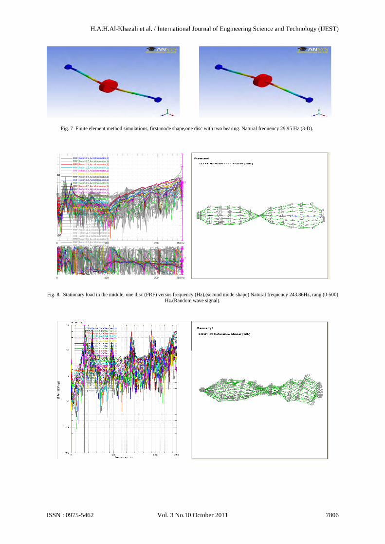
Fig. 7 Finite element method simulations, first mode shape,one disc with two bearing. Natural frequency 29.95 Hz (3-D).

0 250 Hz200100

0 250 Hz200100

FRF(Rotor.0.Y,Accelorometer,1) FRF(Rotor.0.Z,Accelorometer,1) FRF(Rotor.1.Y,Accelorometer,1) FRF(Rotor.1.Z,Accelorometer,1) FRF(Rotor.2.Y,Accelorometer,1) FRF(Rotor.2.Z,Accelorometer,1) FRF(Rotor.3.Y,Accelorometer,1) FRF(Rotor.3.Z,Accelorometer,1) FRF(Rotor.4.Y,Accelorometer,1) FRF(Rotor.4.Z,Accelorometer,1) FRF(Rotor.5.Y,Accelorometer,1) FRF(Rotor.5.Z,Accelorometer,1) FRF(Rotor.6.Y,Accelorometer,1) FRF(Rotor.6.Z,Accelorometer,1) FRF(Rotor.7.Y,Accelorometer,1) FRF(Rotor.7.Z,Accelorometer,1) FRF(Rotor.8.Y,Accelorometer,1) FRF(Rotor.8.Z,Accelorometer,1) FRF(Rotor.9.Y,Accelorometer,1) FRF(Rotor.9.Z,Accelorometer,1) FRF(Rotor.10.Y,Accelorometer,1) FRF(Rotor.10.Z,Accelorometer,1) FRF(Rotor.11.Y,Accelorometer,1) FRF(Rotor.11.Z,Accelorometer,1) FRF(Rotor.12.Y,Accelorometer,1) FRF(Rotor.12.Z,Accelorometer,1) FRF(Rotor.0.Y,Accelorometer,2) FRF(Rotor.0.Z,Accelorometer,2) FRF(Rotor.1.Y,Accelorometer,2) FRF(Rotor.1.Z,Accelorometer,2) FRF(Rotor.2.Y,Accelorometer,2) FRF(Rotor.2.Z,Accelorometer,2) FRF(Rotor.3.Y,Accelorometer,2) FRF(Rotor.3.Z,Accelorometer,2) FRF(Rotor.4.Y,Accelorometer,2) FRF(Rotor.4.Z,Accelorometer,2) FRF(Rotor.5.Y,Accelorometer,2)

1

1

2

2

Fig. 8. Stationary load in the middle, one disc (FRF) versus frequency (Hz),(second mode shape).Natural frequency 243.86Hz, rang (0-500) Hz.(Random wave signal).

20

‐20

0

‐40

40



Fig. 9. Stationary load in the middle, one disc (FRF) versus frequency (Hz), (second mode shape).Natural frequency 242.01Hz rang (0-500)

Hz.(Burst random wave signal).

Fig. 10. Stationary load in the middle, one disc (FRF) versus frequency (Hz),(second mode shape). Natural frequency 244.671Hz rang (0-

500) Hz.(Sine wave signal).

Fig. 11 Finite element method, simulations one disc with two bearing,(Second mode shape).Natural frequency 243.68Hz,(3–D).

3.1.2. Detection damping ratio(ζ) from modal analysis

From Fig .4-11 above we see different excitation input signals for first and second mode shape, one disc in the middle, the rang of band width (0-500)Hz, we see the value of natural frequency closest each other.Table 1-3 show the value of natural frequency (Hz) versus damping ratio (ξ) for shaker test with different excitation input signal (Random, sine& burst random) at sequences and merge all of them in the Fig.12. Relation between mode shape number and natural frequency (Hz) & Fig.13.Relation between damping ratio (ξ ) versus natural frequency (Hz), shaker test.



Clarification the decreased the damping ratio (ζ) caused increased natural frequency until reach maximum amplitude when the system reach resonance ω = ωn, when damping ration (ζ approximately = 0), (free vibration) [6]. Table 1. Shaker test is fixed, accelerometer is roving one disc in the middle (0-500) Hz.Random signal.

Mode shape

No. Natural frequency

(Hz) Damping Ratio(ζ) % Modal A[kg/s] 1 31.25 63.76 4.072554E-06 +i 4.225159E-05 2 243.86 8.44 1.52101E-05 +i7.744734E-05

Table 2. Shaker test is fixed, accelerometer is roving one disc in the middle (0-500) Hz,Sine wave signal.

Mode shape

No. Natural frequency

(Hz) Damping Ratio(ζ) % Modal A[kg/s] 1 30.07 58.32 3.877644E-07 +i0.5665455E-04 2 244.67 6.2 0.1877645E-06 +I0.0667453e-05

Table 3. Shaker test is fixed, accelerometer is roving one disc in the middle (0-500) Hz,Burst Random signal.

Mode shape No.

Natural frequency (Hz) Damping Ratio(ζ) % Modal A[kg/s]

1 31.68 64.77 5.082443E-06 +i 7.335157E-05 2 242..01 7.98 2.36132E-05 +i6.922852E-05

Fig. 12. Relation between mode shape number versus Fig. 13. Relation between damping ratio (ξ ) versus natural frequency natural frequency (Hz), shaker test. (Hz), shaker test. From Table 4. When comparison with hummer technique we see the value approximately equal shown in Fig.14.



Table 4. Comparison experimental value of natural frequency between hammer and shaker test.

Mode shape

Hammer test,ωn(Hz)

Shaker, Random test, ωn (Hz)

Shaker, Sine wave test, ωn (Hz)

Shaker, Burst random test ωn, (Hz)

1 29.79 31.25 30.07 31.68

2 242.74 243.86 244.67 242..01

Fig. 14. Comparison experimental value of natural frequency between hammer with shaker test (different excitation input signals).

3.1.3. Window time record and time record for different of excitation source,shaker test.

Time - s

Re

al N

0 210m100m-4

4

3

2

1

0

-1

-2

-3

A) Windowing time record, Shaker Test, B) Time record sine wave signal, 500HZ. Random signal.

Time - s

Real N

0 212010-4

4

3

2

1

0

-1

-2

-3

Time - s

Am

plit

ud

e N

0 2120100

4

3

2

1

C) Window time record for sin wave 16Hz. D) Window time record for sin wave16Hz.



Frequency - Hz

dB

Re

f 10

1.9

7m

g/N

Ph

ase

de

g

0 252010-40

40

20

0

-20

0 252010-200

200

10050

0-50

Time - s

Re

al N

0 11105-20m

20m

15m

10m

5m

0

-5m

-10m

-15m

E) FRF (Hz), for sine wave 16 Hz. F) Widow Time record sine wave 32 Hz.

Time - s

Am

plit

ud

e g

0 111050

40m

30m

20m

10m

Time - sA

mp

litu

de

g0 11105

0

40m

30m

20m

10m

G) Widow time record sine wave 32 Hz. H) Widow Time record sine wave 50 Hz.

Time - s

Am

plit

ud

e N

0 210m100m0

4

3

2

1

Time - s

Re

al N

0 11105-8m

8m

6m

4m

2m

0

-2m

-4m

-6m

I) Window time record sine wave 50 Hz. J) Time record sine wave 500Hz.

Time - s

Am

plit

ud

e g

0 210m100m0

10

8

6

4

2

Time - s

Am

plit

ud

e N

0 210m100m0

4

3

2

1

K) Random signal 500 Hz. L) Window time record random signal 500Hz.

Fig. 15. Different shapes of (window time record and time record) for different excitation source signal, shaker test;

3.2. Improvement of modelling balancing method (MBM) in rotating mechanism using oscilloscopic 3.2.1. Using oscilloscopic technique to find (amplitude unbalance) 3.2.1.1. Specifications Using oscilloscope type HM 205-3, HAMEG,20 MHz,

Storage scope, HM 205-3 see picture 5 ,below:



Picture 5. Oscillscopic setup[22].

3.2.1.2. Proximity sensor

Beside the accelerometers, one of the other devices which could be used to obtain the response of a system is proximity probes are sensors able to detect the presence of nearby objects without any physical contact. Proximity sensor often emits an electromagnetic or electrostatic field, or abeam of electromagnetic radiation (infrared, for instance), and looks for changes in the field or return signal.

3.2.1.3. Test setup

The test rotor (rotor rig) is shown in picture 6 consist of shaft and two discs, connect proximity sensor with oscillscopic shown in pictuer 5. and increas the speed for different varity and take the result from the screen of oscillscopic.The purpose of generating strength of the movement for the vibration body and the creation of vibration for that with creating a computer when taking readings in public that he was dimensions and introducing it.

3.2.1.4. The outcome results

As it can be seen from the experimental pictures 7-10 ,using oscilloscopic technique,when add 8 gram for each disc of excessive load is added to the loading of the system (in the 25% & 75% from of the effective rotor length),[10], the excessive loading is away from the centre of the shaft by 30 mm ,load added in the disc 1 groove by angle, Ø (45°,225°) degree and in disc 2, Ø (180°,0°) degree, with different speed of rotation, we can prove when add 16 gram mass(8 gram per each disc) at the same conditions and dimensions for two discs, can reduce the amplitude of vibration as well. As it can be seen the results and graphs are matching with each other for approval when add 16 gram mass can reduce vibration amplitude (FRF).That mean the amplitude is reducing in the shaft after add mass in the disc 1 with angle (45°,225°) &in disc 2 with angle (180°, 0°) we expect the noise is reduce as well due to reduce excess vibration.

Picture 6. Schematic of a rotor two discs setup parameter connected with oscilloscopic.

OSCILLOSCOPICADD 16 GRAM MASS



3.2.2. Oscilloscopic results At speed 1000 rpm,without mass. At speed 1000 rpm,with mass. For disc 1, X-direction 2.3 cm. 8 gram, for disc 1, angle 45°, 225° ,X-direction 2.1 cm. For disc 2, Y-direction 1.8 cm. 8 gram for disc 2, angle 180°, 0° , Y-direction 1.5 cm.

A-Without mass1000 rpm. B-With add mass at 1000 rpm.

Picture 7. Amplitude in X, Y direction;

At speed 1500 rpm, without mass. At speed 1500 rpm, with mass. For disc 1, X- direction 1.6 cm. 8 gram, for disc 1, angle 45°, 225° , X-direction1.5cm. For disc 2, Y-direction 1.1 cm. 8 gram for disc 2, angle 180°, 0° , Y-direction 1.0 cm.

A-Without mass at 1500 rpm. B- With add mass at 1500 rpm.

Picture 8. Amplitude in X, Y direction;

At speed 2000 rpm, without mass. At speed 2000 rpm, with mass. For disc 1, X-direction 1.6 cm. 8 gram, for disc 1, X- direction 1.4 cm. For disc 2, Y-direction 1.3 cm. 8 gram, for disc 2, Y-direction 1.1 cm.

A-Without mass at 2000 rpm. B – With add mass at 2000rpm.

Picture 9. Amplitude of FRF in X, Y direction;

At speed 3000 rpm, without mass. At speed 3000 rpm, with mass. For disc 1, X-direction 0.6 cm. 8 gram, for disc 1, angle 45°, 225°, X-direction 0.5 cm. For disc 2, Y-direction 0.4 cm. 8 gram for disc 2, angle 180°, 0°, Y-direction 0.3 cm.



A-Without mass at 3000 rpm. B- With mass at 3000 rpm. Picture 10. Amplitude of FRF in X, Y direction;

4. Discussion and Conclusions In this paper investgate the behaviour of a rotor system with statinary load in effective length (one & two discs ) using different experimental technique. The amplitude of forced vibration can become very large when a frequency component of the excitation source approaches one of the natural frequency of the system particularly fundamental on such as condition is referred to as resonance this is optimal causing failure in both machine and structure,So for this reason is very important for designer have a mean of determine describe of structure.

For shaker test we used different of excitation vibration signals Sine, Sine Swept, Random, Burst Random.

For hammer test we used:- Transient signal only.

Random and Burst random signals give a better coherence and were quicker compared to the sine signal in shaker tests.

Tests with Sine Sweep and Chirp signals could not be completed due to technical difficulties involving the software in shaker tests.

Sine Signals (16, 32 and 50 Hz), gave really bad coherence in shaker tests.

All the signals acquired the mode shapes at 16 and 49 Hz.

Using shaker test for one disc in the middle and find natural frequency and mode shape see Fig. 4-10 experimental for different excitation signal the value close each other show in Table 1-3 and Fig.12-13.This value much close from the value of natural frequency and mode shape when using hammer test clear shown in Table 4 and Fig. 14 for comparison. When using oscilloscopic experimental technique we see the locations of the adding balance masses in suppressing the vibration amplitudes are decided to be at the optimum phase angles for disc 1,of Ø=(45°,225°)& for disc 2, Ø =(180°,0°) and respectively.Is observed for each of the different eccentricity ratios studied.The critical adding mass ratios can also be predicted through its linear relationship with the eccentricity ratios. To conclude the related knowledge as obtained in the study has drawn up a technical basis for better commanding the design quality of the induction motor.The developed solution modules have features of performing multi-purpose rotor dynamic analyses for the characteristics of the rotating machines.The application case addressed in this study has just shown its advantageous strength in solving the realistic problem of the shaft failure for the electric machine.It is especially beneficial for the design of reliable and high quality high-speed spindle machinery by saving the trial and error efforts.Further improvement and validation of the developed software system can solve some other rotating spindle problems such as those potential problems in improving the cutting efficiency by raising the working speeds of the current ultra high speed gas bearing spindles. Comparison with another technique using oscilloscopic picture 7-10 we can prove when add 16 gram mass(8 gram per each disc) at the same condition and dimension for two discs can reduce the amplitude of vibration as well, perfectly nearby to approval values shown the effect of the(MBM) modelling balancing method.The results showed that the (MBM) method could reduce the vibration near the first critical speed sharply while keeping the vibration at working speed at a proper level, so the non-linear constraints was an effective way to make the balancing machinery run-up safely. As a result (MBM) can reduce the vibration more effectively.



The purpose of the modified (MBM) described in this paper is to solve real-world engineering problems using the limited (FRF) data, engineers obtain the equivalent substructure model while avoiding tedious FE modelling processes.By associating the method with other applications, it can have a wide range of practical advantages, such as developing the online diagnostics of rotor system by improving its computer simulation efficiency.

Acknowledgments The author is deeply appreciative support derived from the Iraqi Ministry of Higher Education, Iraqi cultural attaché in London and Kingston University for supporting this research. References [1] Jimin, He.; Zhi-Fang, Fu., (2001) . Modal analysis, Active Oxford, Butterworth-Heinemann, Oxford. [2] Bucher, I., Ewins, D.J., (2001): Modal analysis and testing of rotating structures, Philosophical Transactions of The Royal Society of

London Series A-Mathematical Physical and Engineering Sciences, 359, pp. 61–96, 1778,. [3] Comstock,T.R.,(1999):Improving exciter performance in modal testing ,Proceedings of the 17the International Modal Analysis

Conference ,Kissimmee, pp.1770-1775,FL,U.S.A. [4] Potter, R. ;Richardson, M.H.,( May 1974) :Identification of the modal properties of an elastic structure from measured transfer

function data, 20th International Instrumentation Symposium, Albuquerque, New Mexico. [5] M +P International, SO Analyser Operating Manual. [6] Singiresu, S. Rao., (2005),Mechanical vibrations, Prentice-Hall, Inc.Si Edition ,Singapore. [7] Shliu, Liangsheng Qu.,(2006): Anew field balancing method of rotor systems based on holospectrum and genetic algorithm, Journal of

(Applied soft computing , 8,pp.446-455.Available online at ,www .Science direct.com. [8] Qu, L.S.; H.Qiu .Xu.,(1998): Rotor balancing based holospectrum analysis: principle and practice,China, Mechanical Engineering

9,pp.60-63,(in Chinese).. [9] Arakelian,V. ; Ghazaryan, S.,(Accepted 8 May 2008):Improvement of balancing accuracy of robotic systems: application to leg

orthosis for rehabilitation devices”, Journal of Mechanism and Machine Theory, vol.43, pp.565-575. [10] Bentley Nevada., (2002):Rotor Kit, Part Number 126376-01, Revision, J, Bentley Nevada LLC, U.S.A. [11] Lalanne, M.; Ferraris, G. (1998).Rotor dynamics prediction in engineering, publishing by John Wiley & Sons Ltd, 2nd edition,

England. [12] http://www.mpihome.com/ [13] Muszynska, A.,(1989) :Shaft vibration versus shaft stress, orbit , BNC, 10(3), U.S.A, [14] Ginsberg J H (2001):Mechanical and structural vibration, theory and applications, Georgia Institute of Technology,John Wily &

Sons,Inc, United States. [15] Ewins, D. J.,(1995) . Modal testing: theory and practice, John wily, Exeter, England. [16] ANSYS 12 Help Menu (can be found with ANSYS 12). [17] Rocklin, G.T.;Crowley, J.and Vold, H.,(January 1985): A Comparison of H1, H2, and HV frequency response functions, International

Modal Analysis Conference, 3rd, Orland FL. [18] Reynolds, P. ;, Pavice, A ., (2000) : Impulse hammer versus shaker excitation for the modal testing of building, Floors, Experimental

Techniques 24(3) :39-44. [19] Muszynska, A., (1986) :Fundamental response of rotor, BNC/ BRDRC, Report 1/86, pp. 1-22. [20] Swanson, E. , Powll, C. D. and Weismann, S., (1991):A practical review of rotating machinery critical speeds and modes.12(11):91-

100. [21] Ferraris, G., Maisonneuve, V. and Lalanne, M., (1996) :Prediction of the dynamic behaviour of non symmetric coaxial co or counter

–rotating rotor . Journal Sound vibration 195(4), pp.776-788. [22] http://www.google.co.uk/images?hl=en&rlz=1I7GGLL_enGB&q=oscilloscope&um=1&ie=UTF-8&source=og&sa=N&tab=wi



experimental technique to investigate … · result.the objective of the paper is using modal...

Documents