Turbulence, Heat and Mass Transfer 7 © 2012 Begell House, Inc.

1

Experimental measurement and RANS modelling of multiphase CO2 jet releases R.M. Woolley1, C. Proust2, M. Fairweather1, S.A.E.G. Falle3, J. Hebrard2, D. Jamois2 and C.J. Wareing1 1School of Process, Environmental and Materials Engineering, and 3School of Mathematics, University of Leeds, Leeds LS2 9JT, UK, r.m.woolley@leeds.ac.uk, m.fairweather@leeds.ac.uk, s.a.e.g.falle@leeds.ac.uk, c.j.wareing@leeds.ac.uk 2INERIS, Dept. PHDS, Parc Technologique ALATA, BP 2, 60550 Verneuil-en-Halatte, France, christophe.proust@ineris.fr, jerome.hebrard@ineris.fr, didier.jamois@ineris.fr  

Abstract – The deployment of a complete carbon-capture and storage chain requires a focus upon the hazards posed by the operation of CO2 pipelines, and the consequences of accidental release must be considered as an integral part of the design process. CO2 poses a number of dangers upon release due to its physical properties, and modelling of the fluid dynamics of such poses a unique set of problems due to its unusual phase transition behaviour. Additionally, few experimental observations have been made with regard to CO2 releases to date, and so the physics and thermochemistry of such systems are not well understood. The current work has involved state-of-the-art mathematical modelling and experimental measurement to further advances in this area of research, and presented here are results from both. The performance of the mathematical models is elucidated with the use of the experimental data, and avenues for future developments are presented. 1. Introduction The CO2PipeHaz project [1] aims to address the fundamentally important and urgent issue regarding the accurate prediction of fluid phase, discharge rate, emergency isolation and subsequent atmospheric dispersion occurring during accidental releases from pressurised CO2 pipelines. Such pipelines are considered to be the most likely method for transportation of captured CO2 from power plants and other industries prior to subsequent storage, and their safe operation is of paramount importance as their contents are likely to be in the region of several thousand tonnes. CO2 poses a number of dangers upon release due to its physical properties. It is a colourless and odourless asphyxiant which has a tendency to sublimation and solid formation, and is directly toxic if inhaled in air at concentrations around 5%, and likely to be fatal at concentrations around 10%.

The modelling of CO2 fluid dynamics poses a unique set of problems due to its unusual phase transition behaviour and physical properties. Liquid CO2 has a density much greater than water, but has a viscosity of magnitude more frequently associated with gases. These properties make the transport of supercritical CO2 an economically viable and attractive proposition. However, due to it possessing a relatively high Joule-Thomson expansion coefficient, preliminary calculations and experimental evidence indicate that the rapid expansion of an accidental release may reach temperatures below -100°C. Due to this effect, solid formation following a pipeline puncture or rupture is to be expected, whether directly from liquid or via a vapour-solid phase transition. Additionally, CO2 sublimes at ambient atmospheric conditions, which is behaviour not seen in most other solids, and is an important consideration when assessing the hazards of flows such as these.

Turbulence, Heat and Mass Transfer 7

2

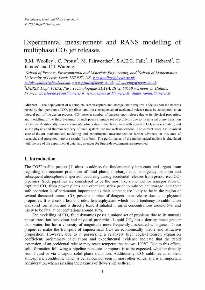
The developments presented in this paper concern the measurement of medium-scale jet releases of CO2, and the formulation of a multi-phase heterogeneous discharge and dispersion model capable of predicting the near-field fluid dynamic and phase behaviour of such CO2 releases. Predicting the correct fluid phase during the discharge process in the near-field is of particular importance given the very different hazard profiles of CO2 in the gas and solid states. Model validations have also been undertaken using the experimental data described, with shortcomings of the mathematical model elucidated through such comparisons, and suggestions for further developments presented. 2. Experimental Measurements Figure 1 displays the experimental rig located at the INERIS test site, which incorporates a 2

cubic metre spherical pressure vessel. This is thermally insulated, and can contain up to 1000 kg of CO2 at a maximum operating pressure and temperature of 200 bar and 200 ºC, respectively. It is equipped internally with 6 thermocouples and 2 high precision pressure gauges as well as sapphire observation windows. It is connected to a discharge line of 50 mm inner diameter, with no internal restrictions. In total, the line is 9 m long including a bend inside the vessel, plunging to the bottom in order to ensure that it is fully submersed in liquid CO2. Three full-bore ball valves are installed in the pipe. Two are positioned close to the vessel and the third near to the orifice holder. The first valve

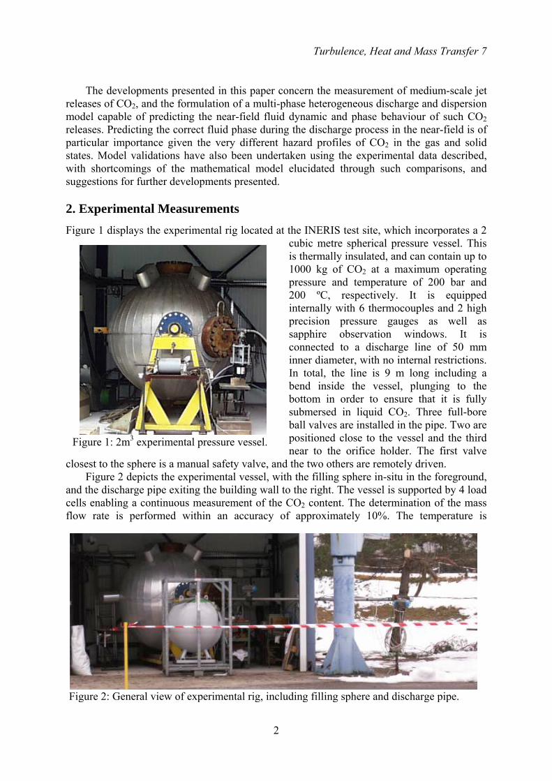
closest to the sphere is a manual safety valve, and the two others are remotely driven. Figure 2 depicts the experimental vessel, with the filling sphere in-situ in the foreground,

and the discharge pipe exiting the building wall to the right. The vessel is supported by 4 load cells enabling a continuous measurement of the CO2 content. The determination of the mass flow rate is performed within an accuracy of approximately 10%. The temperature is

Figure 1: 2m3 experimental pressure vessel.

Figure 2: General view of experimental rig, including filling sphere and discharge pipe.

R.M. Woolley et al.

3

measured inside the vessel and immediately upstream of the orifice with 0.5 mm K type thermocouples of accuracy better than 1 °C. The static pressure is measured inside the vessel using a Kistler 0-200 bar instrument with an accuracy of ±0.1%, and immediately upstream from the orifice using a KULITE 0-350 bar instrument with an accuracy of ±0.5%. The vessel instrumentation is shown in Figure 3.

Various orifices can and are used at the exit plane of the discharge pipe, and are all

drilled into a large screwed flange. The thickness of this flange is typically 15 mm and the diameter of the orifice is constant over a length of 10 mm and then expanded with an angle of 45° towards the exterior. Figure 4

provides an example of such a nozzle, whilst Figure 5 is a high-speed camera still of a typical release from a 9 mm nozzle. The discharge nozzle diameters used were 9, 12 and 25mm in the three tests reported and studied here.

Figure 3: Vessel instrumentation.

Figure 4: Example of orifice flange.

Figure 5: Camera still of a 9 mm

Turbulence, Heat and Mass Transfer 7

4

Table 1: Parameters of the experimental releases.

Test Number

Ambient Temperature

/ K

Air Humidity

/ %

Reservoir Pressure /

bar

Nozzle Diameter /

mm 6 276.15 95.0 95 9 7 279.15 95.0 85 12 8 277.15 95.0 77 25

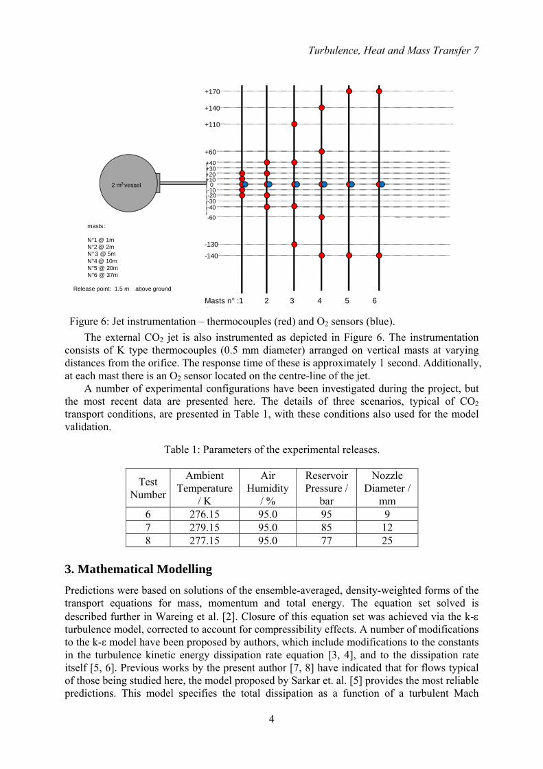
The external CO2 jet is also instrumented as depicted in Figure 6. The instrumentation consists of K type thermocouples (0.5 mm diameter) arranged on vertical masts at varying distances from the orifice. The response time of these is approximately 1 second. Additionally, at each mast there is an O2 sensor located on the centre-line of the jet.

A number of experimental configurations have been investigated during the project, but the most recent data are presented here. The details of three scenarios, typical of CO2 transport conditions, are presented in Table 1, with these conditions also used for the model validation.

3. Mathematical Modelling Predictions were based on solutions of the ensemble-averaged, density-weighted forms of the transport equations for mass, momentum and total energy. The equation set solved is described further in Wareing et al. [2]. Closure of this equation set was achieved via the k-ε turbulence model, corrected to account for compressibility effects. A number of modifications to the k-ε model have been proposed by authors, which include modifications to the constants in the turbulence kinetic energy dissipation rate equation [3, 4], and to the dissipation rate itself [5, 6]. Previous works by the present author [7, 8] have indicated that for flows typical of those being studied here, the model proposed by Sarkar et. al. [5] provides the most reliable predictions. This model specifies the total dissipation as a function of a turbulent Mach

 

2 m3 vessel 

masts :

N°1 @ 1mN°2 @ 2mN° 3 @ 5mN°4 @ 10m N°5 @ 20mN°6 @ 37m

0 +20 +30 

+110

+140

+170

-20- 30- 40

- 60

-130

-140

+40 +60

Masts n° :1 2 3 4 5 6

- 10

+10

Release point: 1.5 m above ground

Figure 6: Jet instrumentation – thermocouples (red) and O2 sensors (blue).

R.M. Woolley et al.

5

number and was derived from the analysis of a direct numerical simulation of the exact equations for the transport of the Reynolds stresses in compressible flows. Observations made of shock-containing flows indicated that the important sink terms in the turbulence kinetic energy budget generated by the shocks were a compressible turbulence dissipation rate, and to a lesser degree, the pressure-dilatation term. In isotropic turbulent flow, the pressure-dilatation term was found to be negligibly small, and so it was proposed that correction only be made to the dissipation rate using a function of the turbulent Mach number as: 2

c tCMε ε= (1) where the constant C is set to unity to allow for the neglected pressure-dilatation term and

tM is the turbulent Mach number. The application to the k-ε model is then made by modification to the source term of the turbulence energy evolution equation and to the turbulence viscosity. as defined by Equations 2 and 3 respectively: 2

k tW Mρ ε= − (2)

2

2(1 )tt

kCMμμ ρ

ε=

+ (3)

The turbulent Mach number is defined as:

( )1

22t

kM

a= (4)

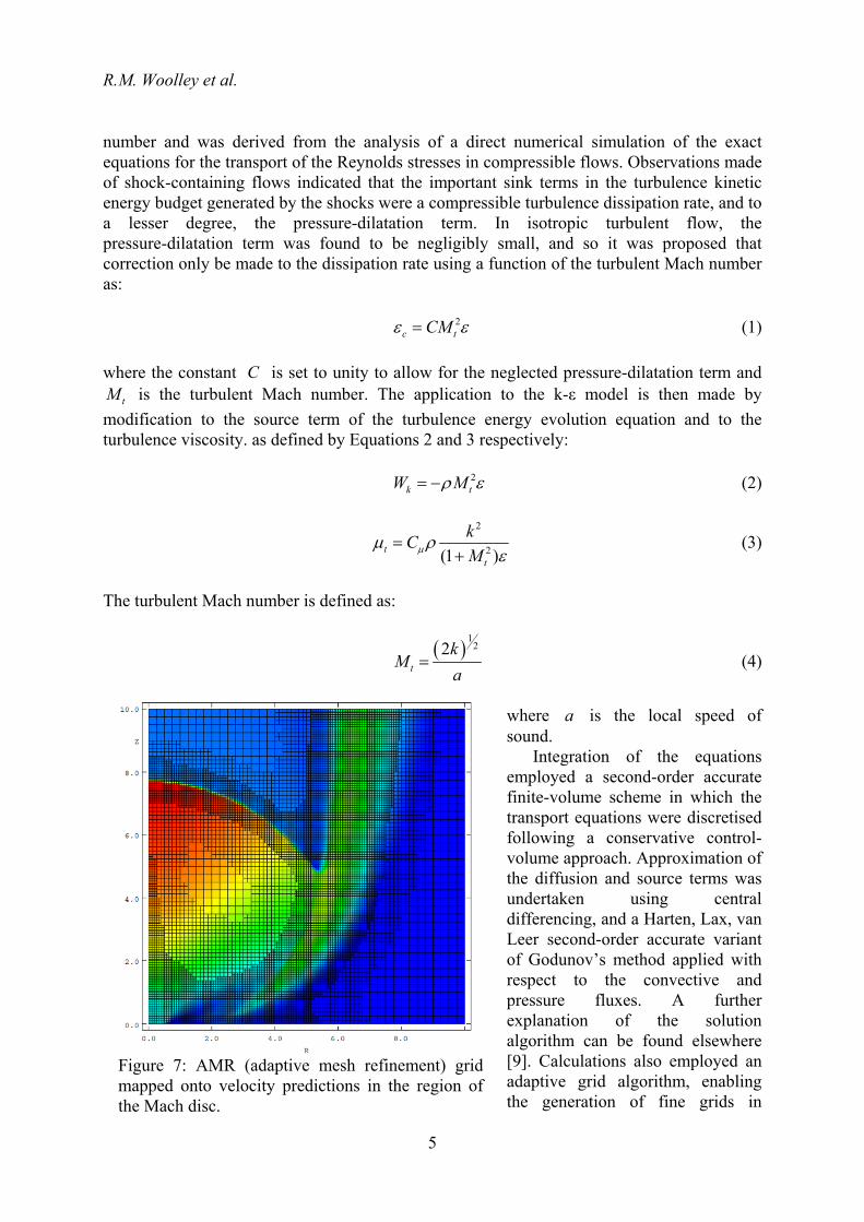
where a is the local speed of sound. Integration of the equations employed a second-order accurate finite-volume scheme in which the transport equations were discretised following a conservative control- volume approach. Approximation of the diffusion and source terms was undertaken using central differencing, and a Harten, Lax, van Leer second-order accurate variant of Godunov’s method applied with respect to the convective and pressure fluxes. A further explanation of the solution algorithm can be found elsewhere [9]. Calculations also employed an adaptive grid algorithm, enabling the generation of fine grids in

Figure 7: AMR (adaptive mesh refinement) grid mapped onto velocity predictions in the region of the Mach disc.

Turbulence, Heat and Mass Transfer 7

6

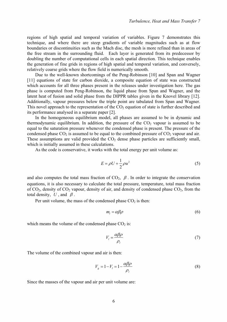
regions of high spatial and temporal variation of variables. Figure 7 demonstrates this technique, and where there are steep gradients of variable magnitudes such as at flow boundaries or discontinuities such as the Mach disc, the mesh is more refined than in areas of the free stream in the surrounding fluid. Each layer is generated from its predecessor by doubling the number of computational cells in each spatial direction. This technique enables the generation of fine grids in regions of high spatial and temporal variation, and conversely, relatively coarse grids where the flow field is numerically smooth.

Due to the well-known shortcomings of the Peng-Robinson [10] and Span and Wagner [11] equations of state for carbon dioxide, a composite equation of state was constructed which accounts for all three phases present in the releases under investigation here. The gas phase is computed from Peng-Robinson, the liquid phase from Span and Wagner, and the latent heat of fusion and solid phase from the DIPPR tables given in the Knovel library [12]. Additionally, vapour pressures below the triple point are tabulated from Span and Wagner. This novel approach to the representation of the CO2 equation of state is further described and its performance analysed in a separate paper [2].

In the homogeneous equilibrium model, all phases are assumed to be in dynamic and thermodynamic equilibrium. In addition, the pressure of the CO2 vapour is assumed to be equal to the saturation pressure whenever the condensed phase is present. The pressure of the condensed phase CO2 is assumed to be equal to the combined pressure of CO2 vapour and air. These assumptions are valid provided the CO2 dense phase particles are sufficiently small, which is initially assumed in these calculations.

As the code is conservative, it works with the total energy per unit volume as:

212

E U uρ ρ= + (5)

and also computes the total mass fraction of CO2, β . In order to integrate the conservation equations, it is also necessary to calculate the total pressure, temperature, total mass fraction of CO2, density of CO2 vapour, density of air, and density of condensed phase CO2, from the total density, U , and β .

Per unit volume, the mass of the condensed phase CO2 is then: lm αβρ= (6)

which means the volume of the condensed phase CO2 is:

ll

V αβρρ

= (7)

The volume of the combined vapour and air is then:

1 1g ll

V V αβρρ

= − = − (8)

Since the masses of the vapour and air per unit volume are:

R.M. Woolley et al.

7

( ) ( )1 , 1v am mβ α ρ β ρ= − = − (9) their densities are then:

( )1

1

vv

g

l

mV

β α ρρ

αβρρ

−= =

⎛ ⎞−⎜ ⎟

⎝ ⎠

and ( )1

1

aa

g

l

mV

β ρρ

αβρρ

−= =

⎛ ⎞−⎜ ⎟

⎝ ⎠

(10)

Since the CO2 vapour is in equilibrium with the solid/liquid CO2, we have:

( ) ,vs

v

mp T p Tρ

⎛ ⎞= ⎜ ⎟

⎝ ⎠ (11)

where ( ),vp Tρ is the pressure given by the equation of state. In regions where there is significant mixing, one can use the ideal equation of state for the CO2 vapour and:

( ), vv

v

R Tp Tmρρ = (12)

The total pressure is then given by:

a v

a v

p RTm mρ ρ⎛ ⎞

= +⎜ ⎟⎝ ⎠

(13)

and the total internal energy by:

( )( )

( )( ) ( )1 1

,1 1 l

v v a a

U RT U Tm mβ α β

αβ ργ γ

⎡ ⎤− −= + +⎢ ⎥− −⎣ ⎦

(14)

where ( ),lU Tρ is the internal energy per unit mass of condensed phase CO2. The solid density is then determined from: ( ),l l p Tρ ρ= (15) which is obtained from the equation of state. Equations 10 to 15 are solved for T , p and α using a Newton-Raphson iteration.

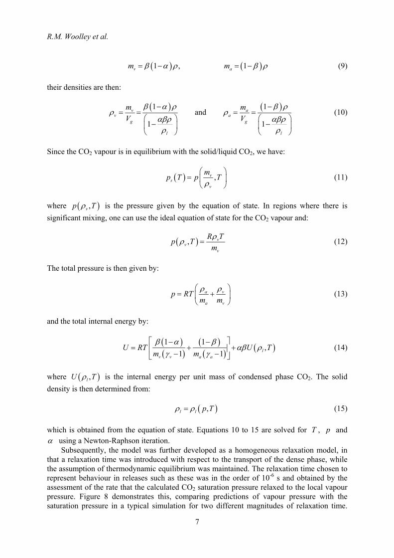
Subsequently, the model was further developed as a homogeneous relaxation model, in that a relaxation time was introduced with respect to the transport of the dense phase, while the assumption of thermodynamic equilibrium was maintained. The relaxation time chosen to represent behaviour in releases such as these was in the order of 10-6 s and obtained by the assessment of the rate that the calculated CO2 saturation pressure relaxed to the local vapour pressure. Figure 8 demonstrates this, comparing predictions of vapour pressure with the saturation pressure in a typical simulation for two different magnitudes of relaxation time.

Turbulence, Heat and Mass Transfer 7

8

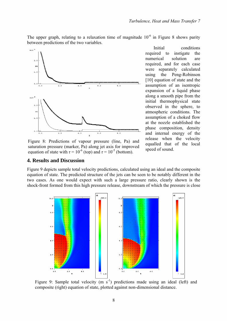
Figure 9: Sample total velocity (m s-1) predictions made using an ideal (left) and composite (right) equation of state, plotted against non-dimensional distance.

The upper graph, relating to a relaxation time of magnitude 10-6 in Figure 8 shows parity between predictions of the two variables.

Initial conditions required to instigate the numerical solution are required, and for each case were separately calculated using the Peng-Robinson [10] equation of state and the assumption of an isentropic expansion of a liquid phase along a smooth pipe from the initial thermophysical state observed in the sphere, to atmospheric conditions. The assumption of a choked flow at the nozzle established the phase composition, density and internal energy of the release when the velocity equalled that of the local speed of sound.

4. Results and Discussion Figure 9 depicts sample total velocity predictions, calculated using an ideal and the composite equation of state. The predicted structure of the jets can be seen to be notably different in the two cases. As one would expect with such a large pressure ratio, clearly shown is the shock-front formed from this high pressure release, downstream of which the pressure is close

Figure 8: Predictions of vapour pressure (line, Pa) and saturation pressure (marker, Pa) along jet axis for improved equation of state with τ = 10-6 (top) and τ = 10-5 (bottom).

R.M. Woolley et al.

9

160

180

200

220

240

260

280

300

Tem

pera

ture

/ K

Test 7x = 1md = 85

160

180

200

220

240

260

280

300

Tem

pera

ture

/ K

Test 7x = 2md = 170

-1.2 -0.8 -0.4 0.0 0.4 0.8 1.2

160

180

200

220

240

260

280

300

Tem

pera

ture

/ K

y / m

Test 7x = 5md = 424

Figure 11: Radial temperature profiles of Test 7 at axial distances of 1, 2 and 5 m (lines – calculations, symbols – data).

160

180

200

220

240

260

280

300Te

mpe

ratu

re /

K

0 5 10 15 200.2

0.4

0.6

0.8

1.0

CO

2 den

se-p

hase

frac

tion

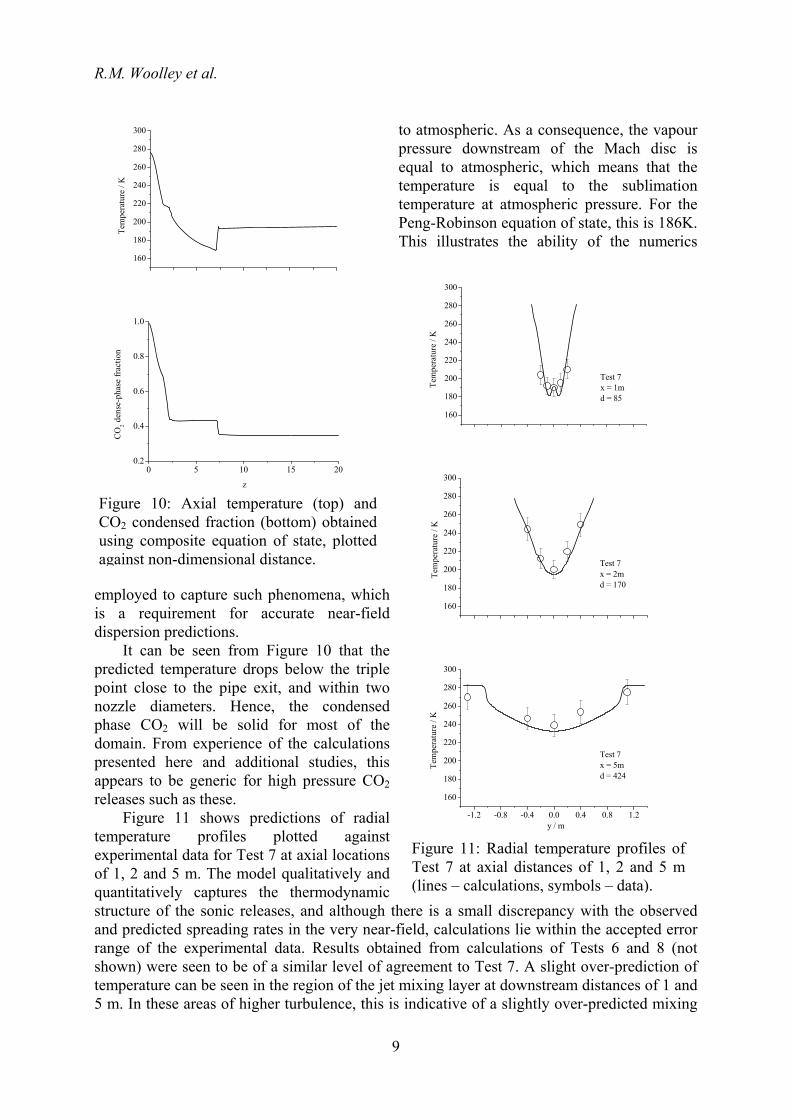
z Figure 10: Axial temperature (top) and CO2 condensed fraction (bottom) obtained using composite equation of state, plotted against non-dimensional distance.

to atmospheric. As a consequence, the vapour pressure downstream of the Mach disc is equal to atmospheric, which means that the temperature is equal to the sublimation temperature at atmospheric pressure. For the Peng-Robinson equation of state, this is 186K. This illustrates the ability of the numerics

employed to capture such phenomena, which is a requirement for accurate near-field dispersion predictions.

It can be seen from Figure 10 that the predicted temperature drops below the triple point close to the pipe exit, and within two nozzle diameters. Hence, the condensed phase CO2 will be solid for most of the domain. From experience of the calculations presented here and additional studies, this appears to be generic for high pressure CO2 releases such as these.

Figure 11 shows predictions of radial temperature profiles plotted against experimental data for Test 7 at axial locations of 1, 2 and 5 m. The model qualitatively and quantitatively captures the thermodynamic structure of the sonic releases, and although there is a small discrepancy with the observed and predicted spreading rates in the very near-field, calculations lie within the accepted error range of the experimental data. Results obtained from calculations of Tests 6 and 8 (not shown) were seen to be of a similar level of agreement to Test 7. A slight over-prediction of temperature can be seen in the region of the jet mixing layer at downstream distances of 1 and 5 m. In these areas of higher turbulence, this is indicative of a slightly over-predicted mixing

Turbulence, Heat and Mass Transfer 7

10

0 1 2 3 4 5 6

160

180

200

220

240

260

280

300

x / m

Tem

pera

ture

/ K

Test 6y = 0m

0 1 2 3 4 5 6

x / m

Test 7y = 0m

Figure 12: Centre-line temperature profiles of Tests 6 and 7 (lines – calculations, symbols – data).

0 1 2 3 4 5 60

5

10

15

20

25

x / m

O2 /

% v

/v

Test 6y = 0m

0 1 2 3 4 5 6

x / m

Test 7y = 0m

Figure 13: Centre-line O2 percentage profiles of Tests 6 and 7 (lines – calculations, symbols – data).

rate. The k-ε turbulence model is well known to underperform in such a manner in compressible jets such as these, and although corrected according to the model of Sarkar et al. [5] there is the possibility of an anisotropic element of the Reynolds-stress tensor not being accounted for. Hence, a second-moment turbulence closure is currently being incorporated within the overall model. Within the core of the jet, temperatures are seen to be slightly under-predicted when compared to experiment, except in the inviscid region still present at 1 m. It is possible that dense phase CO2 is removed from the system due to such phenomena as agglomeration, which would affect the higher temperatures observed. Hence, current developments of the model include the incorporation of sub-models for the distribution of solid and liquid particles within the flow, and it is expected that the effects of phenomena such as particle coagulation will have an impact upon the predicted temperatures. Also, the system may not be in equilibrium due to this, or the generated turbulence, which may cause the observed discrepancies.

Figure 12 depicts axial profiles of temperature predictions plotted against experimental data along the centre-line in the CO2 releases of Tests 6 and 7. As previously discussed, the level of agreement between calculation and experiment is comparable for these two investigations. Also reflected is the observed centre-line under-prediction of temperature common to all investigated cases.

Figure 13 displays predictions of O2 percentage content plotted against experimental data on the centre-line of the same Tests as addressed in Figure 12. The evident over-prediction of the volumetric percentage at first appears counter-intuitive with respect to the

R.M. Woolley et al.

11

under-prediction of temperature. However, it is indicative of the two possible competing sources of error within the calculations. As previously discussed, the possible over-prediction of mixing due to the isotropic assumption of the turbulence model is liable to produce temperature and O2 over-prediction. In opposition, energy may be removed from the CO2 jet due to solid formation and possible rainout and subsequent sublimation.

5. Conclusions Presented are experimental observations of the structure of high pressure releases of multi-phase carbon dioxide representative of medium scale releases arising from an accidental pipeline puncture or rupture. Additionally, a computational fluid dynamic model capable of predicting the near-field structure of these releases is presented, with the model in part validated against the new experimental data. The model developed has yielded an excellent level of agreement with predictions of the characteristics of these jets in comparison with temperature, and good agreement with composition data for a number of comparisons with experimentally derived data.

It has been identified that two areas of improvement are required to ensure accurate representation of the complex physics observed in these release scenarios. Firstly, a second-moment turbulence model is required to represent the turbulence anisotropy, which is expected to correct the over-prediction of mixing due to the two-equation model implemented. Secondly, the inclusion of particles within a Lagrangian framework is required to more accurately represent the thermophysical interactions between the physical phases. Due to these conclusions, developmental work is ongoing to address these issues.

Additionally, it is clear from the predictions, derived for a dense phase release, that significant solids are generated within the near-field of the jet, despite the pipeline containing no dry ice. This is an important conclusion with respect to the future design of CO2 pipelines and the consideration of the related hazards. Nomenclature Roman letters: a local sound speed R universal gas constant C model constant T temperature d non-dimensional distance u velocity E total internal energy per unit volume U internal energy per unit mass k turbulence kinetic energy V volume m mass W source term M Mach number x axial location p pressure y radial location r non-dimensional radial location z non-dimensional axial location Greek letters: Subscripts: α condensed phase fraction a air β total mass fraction of CO2 c compressible ε dissipation of k g gas γ ratio of specific heats l liquid/solid (condensed phase) μ molecular viscosity s saturation ρ density t turbulent τ relaxation time v vapour

Turbulence, Heat and Mass Transfer 7

12

Acknowledgements The research leading to the findings report has received funding from the European Union Seventh Framework Programme FP7-ENERGY-2009-1 under grant agreement number 241346. This paper reflects only the authors’ views and the European Union is not liable for any use that may be made of the information contained therein. References 1. CO2PipeHaz, CO2PipeHaz quantitative failure consequence hazard assessment for next

generation CO2 pipelines: The missing link, 2011. [cited 21/03/12; CO2PipeHaz Project Website]. Available from: http://www.co2pipehaz.eu/.

2. C.J. Wareing, M. Fairweather, S.A.E.G. Falle, and R.M. Woolley, RANS modelling of sonic CO2 jets. In Turbulence Heat and Mass Transfer 7 (Edited by K. Hanjalic, et al.), Begell House, Inc.: Sicily, Italy, 2012 (to appear).

3. NASA, Computation of Turbulent Flows Using an Extended k-epsilon Turbulence Closure Model. (CR-179204), 1987.

4. A.M.E. Baz. Modelling compressibility effects on free turbulent shear flows. In 5th Biennial Colloquium on Computational Fluid Dynamics. UMIST. 1992.

5. S. Sarkar, G. Erlebacher, M.Y. Hussaini, and H.O. Kreiss. The analysis and modelling of dilatational terms in compressible turbulence. J. Fluid Mech., 227: 473-493, 1991.

6. O. Zeman. Dilational dissipation: The concept and application in modeling compressible mixing layers. Phys. Fluids A-Fluid, 2: 178-188, 1990.

7. M. Fairweather and K.R. Ranson, Modelling of underexpanded jets using compressibility-corrected, k-ε turbulence models. In Turbulence, Heat and Mass Transfer 4 (Edited by K. Hanjalic, Y. Nagano, and M. Tummers), pp. 649-656, Begell House, Inc., 2003.

8. M. Fairweather and K.R. Ranson. Prediction of underexpanded jets using compressibility-corrected, two-equation turbulence models. Prog. Comput. Fluid Dy., 6: 122-128, 2006.

9. S.A.E.G. Falle. Self-similar jets. Mon. Not. R. Astron. Soc., 250: 581-596, 1991. 10. D.-Y. Peng and D.B. Robinson. A new two-constant equation of state. Ind. Eng. Chem.

Fun., 15: 59-64, 1976. 11. R. Span and W. Wagner. A new equation of state for carbon dioxide covering the fluid

region from the triple-point temperature to 1100 K at pressures up to 800 MPa. J. Phys. Chem. Ref. Data, 25: 1509-1596, 1996.

12. Imperial College London, Knovel Library, 2011. [cited 21/11/11]; Available from: http://www3.imperial.ac.uk/library/find/databases/knovellibrary.