experimental investigation of fully developed flows of...
TRANSCRIPT
Experimental Investigation of Fully Developed Flows of a Newtonian Fluid in Straight Rectangular Ducts with
Adjacent Open and Porous-Metal-Foam Domains
by
James Medvescek
Department of Mechanical Engineering
McGill University
Montréal, Québec, Canada
A thesis submitted to McGill University
in partial fulfilment of the requirements for the degree of
Master of Engineering
© James Medvescek, Montréal, Canada, August 2013
ii
Abstract
Over the last two decades, porous metal foams (which have very high values of surface-
area-to-volume ratio, of the order of 10,000 square meters per cubic meter; and values of
porosity in the range 0.85-0.98) have been increasingly used in devices for heat transfer
(ultra-compact heat exchangers and heat sinks; heat pipes; and loop heat pipes), filtration,
catalytic conversion, and acoustical control. In computational methods for thermofluid
optimization of such devices, cost-effective modeling of fluid flows in adjacent open and
porous-metal-foam domains is done using two different, but compatible, sets of volume-
averaged governing equations; and at the interface between these domains, the intrinsic-
phase-averaged pressure, phase-averaged fluid velocity, and normal stress are assumed to
be continuous, and a tangential stress-jump condition, with two adjustable coefficients, is
imposed. Accurate experimental data for determining these adjustable coefficients and
establishing possible laminar-turbulent transition criteria for the aforementioned flows are
urgently needed.
In the present work, an experimental investigation of fully developed flows of air in a
straight, uniform, rectangular duct of high cross-sectional aspect ratio and containing
open and porous-metal-foam domains was undertaken. These flows are akin to those
studied in the classical Beavers-Joseph problem. Four different porous metal foams (with
nominal pores per inch designations of 20, 40, 60; nominal thickness of 12.7 mm; and
porosity in the range 0.85-0.94) were considered. An experimental facility was specially
designed and constructed to allow test-section configurations of nominal open-domain
heights of 0 (completely filled with porous metal foams), 3.175 mm, 6.35 mm, and
12.7 mm. The nominal width and length of the test section was fixed at 152.4 mm and
457.2 mm, respectively. The top wall of the test section had 64 wall-static-pressure taps
and also a wall-shear-stress sensor, which was redesigned (improved) from an earlier
version. The airflow rates were measured using a Venturi tube (specially designed,
constructed, and calibrated for this work) and a bank of laminar flow elements. An
analytical solution for laminar fluid flows in the problems of interest was adapted from
other works in the published literature.
iii
The results obtained from experiments undertaken for benchmarking tasks,
characterization of the porous metal foams (photomicrographs; ligament, pore, and cell
effective diameters; and porosity), and calibration of the wall-shear-stress sensor are
presented and discussed. Data from experiments undertaken to determine the permeability
and dimensionless form-drag coefficient of the porous metal foams were processed using
four different approaches, and the results are presented and comparatively discussed.
Comprehensive sets of experimental data collected for airflows in adjacent open and
porous-metal-foam domains (in the laminar, transitional, and turbulent regimes) are
presented and discussed. These experimental data, the analytical solution for such
problems with laminar flows, power-spectral-density (PSD) plots of the instantaneous
wall-shear-stress measurements, and the requirements for physically tenable values for
the laminar-flow results were collectively used to obtain guidance regarding laminar-
turbulent transition, and then deduce the two coefficients in the interfacial jump condition
on the shear stress.
For flows through test sections completely filled with the porous metal foams, the data
collected were used to obtain a Darcy friction factor as a function of a Reynolds number
(both based on the superficial velocity of the air and the effective diameter of the metal-
foam ligaments). The data collected in the experiments on flows in test sections with
adjacent open and porous domains were used to obtain the open-domain Darcy friction
factor as a function of the corresponding Reynolds number. These results are presented
and discussed.
iv
Résumé
Au cours des deux dernières décennies, les mousses métalliques poreuses, MMP, (ayant
des valeurs très élevées de superficie d’échange thermique volumétrique, de l'ordre de
10 000 mètres carrés par mètre cube, et valeurs de la porosité de 0,85 à 0,98) sont
devenues de plus en plus commun dans plusieurs domaines: le transfert thermique
(échangeurs de chaleur ultracompacts, dissipateurs de chaleur, caloducs et des caloducs
en boucle), la filtration; la conversion catalytique; et l’acoustique. Les simulations
numériques d’écoulements en domaines ouvert / de MMP adjacents se font en résolvant
deux équations différentes (moyennées volumétriquement), correspondant aux deux
domaines différents. À l'interface de ceux-ci, la pression intrinsèque (moyennée), la
vélocité du fluide (moyenné), et la contrainte normale sont supposées être continues, et
une discontinuité de la contrainte tangentielle à l'interface, avec deux coefficients
réglables, est imposée. La connaissance de ces coefficients réglables, et l’établissement de
critères de transition laminaire-turbulent pour ces types d’écoulements nécessitent
urgemment des données expérimentales précises.
Le travail ci-inclus comprend une étude expérimentale d’écoulements d'air pleinement
développés, en canal rectangulaire et uniforme, de rapport largeur/hauteur élevé, et
contenant des domaines ouvert / de MMP adjacents. De tels écoulements ressemblent à
ceux étudiés dans le problème Beavers-Joseph. Quatre MMP différentes (ayant des pores
de tailles nominaux de 20, 40, 60 pores par pouce, une épaisseur nominale de 12,7 mm, et
des porosités allant de 0,85 à 0,94) furent examinées. Un dispositif expérimental fut
conçu et construit pour permettre des configurations d'hauteurs du domaine ouvert dans la
section de mesure de 0 (complètement rempli de MMP), 3,175 mm, 6,35 mm, et
12,7 mm. La largeur nominale et la longueur de la section de mesure furent fixées à
152,4 mm et 457,2 mm, respectivement. La paroi supérieure de la section de mesure
possède 64 prises de pression statique et un capteur de contrainte de cisaillement à la
paroi. Les débits d'air furent mesurés en utilisant un tube de Venturi (spécialement conçu,
construit, et étalonné pour ce travail) et une banque d'éléments laminaires.
v
Les résultats obtenus des expériences menées pour i) des tâches d'analyse comparative; ii)
la caractérisation des mousses métalliques (microphotographes; diamètres effectifs des
ligaments, des pores et des cellules; porosité); et iii) l’étalonnage du capteur de contrainte
de cisaillement sont présentés et interprétés. Les données provenant des expériences
mesurant la perméabilité et le coefficient adimensionnel de traînée de forme des MMP
furent déterminées selon quatre approches différentes, et comparées.
Des ensembles de données expérimentales recueillies en écoulements d’air en domaines
ouvert / poreux adjacents (dans les régimes laminaire, de transition, et turbulent) furent
présentés et analysés. Ces données, la solution analytique de tels écoulements laminaires,
les densités spectrales de puissance des mesures instantanées de la contrainte de
cisaillement à la paroi, et les conditions nécessaires correspondantes au régime laminaire
furent collectivement utilisées pour obtenir des indicateurs concernant la transition
laminaire-turbulent, et pour déduire les deux coefficients dans la condition de
discontinuité de la contrainte de cisaillement à l'interface.
Les données provenant des mesures dans lesquelles le canal était complètement rempli de
MMP furent utilisées pour calculer un coefficient de frottement de Darcy en fonction du
nombre de Reynolds (basé sur la vélocité superficielle de l'air et le diamètre effectif des
ligaments de la MMP). Les données recueillies dans les expériences en domaines
ouverts / poreux adjacents furent utilisées pour obtenir le coefficient de frottement de
Darcy (du domaine ouvert) en fonction du nombre de Reynolds correspondant. Ces
résultats sont présentés et interprétés.

vi
I dedicate this thesis to my uncle
Karl Dusan Medvescek
1957-2012

vii
Acknowledgements
I would like to express my sincerest gratitude to both of my supervisors, Professor B.
Rabi Baliga and Professor Laurent B. Mydlarski, for accepting me to be one of their
students, and for offering me such an interesting, and challenging thesis project. Both of
your continual support and guidance throughout my M.Eng. studies has been greatly
appreciated, and I have most certainly learned a great deal from both of you.
I would also like to thank the Natural Sciences and Engineering Research Council
(NSERC) of Canada, the Fonds de recherche du Québec - Natures et technologies
(FRQNT), McGill University, and my two supervisors, for providing me with financial
support throughout the course of my studies.
I would especially like to thank my lab partner and friend, Samer Afara, for working with
me to redesign the wall-shear-stress sensor he had designed and built earlier, in his
M.Eng. work. Your inputs were significant contributions to this work, and our new sensor
was a key element to obtaining excellent data.
To my parents, Ingo and Mary, my brothers, Alex and Nick, the rest of my family, and to
my friends, Kyran, Mike, Eric, Adam, and Nicky, your continual support and
encouragement throughout my studies has been tremendous. To my girlfriend, Anouk,
your patience, love, understanding, and encouragement have been absolutely amazing
during my Master’s. I also very much appreciate the visits (and bringing me some
dinners) during my extremely long measurement days.
This project could not have been completed were it not for Mr. Chunilal Mistry, his son
Bhavesh, and his employees at the Bhavesh Machine Shop, who machined the air
channel, transition box, Venturi tube, and wall-shear-stress sensor components. I would
also like to thank the technical staff of the Faculty of Engineering, especially Antonio
(Tony) Micozzi, Andy Hofmann, and Mathieu Beauchesne for their inputs and help in
machining the metal foam test sections. Many thanks to Professor Larry Lessard and

viii
Professor Pascal Hubert for kindly granting me access to the Composites Laboratory and
the oven there for heat-curing the epoxies used in attaching the metal foam to the test
sections.
For their technical support and inputs, I would like to thank the following people: Jean-
Pierre Bessette and Martin Richer from Polycontrols Inc.; Cassidy Clark from Erg
Aerospace; Mark Heamon from Selee Corporation; Charles Clement from Crystex
Composites LLC; Ariel Kemer for expertly welding the Venturi tube connections; and
Éric Dubé from WeldPro Inc.
For help with a number of formalities of graduate school and thesis submission tasks,
thanks go to Ms. Emily McHugh and Ms. Joyce Nault.
Last, but not least, I would also like to thank my other lab partners for their support,
Jeffrey Poissant, Nirmalakanth (Nirma) Jesuthasan, Alexandre Lamoureux, Brandon
Tulloch, Laura Yakuma, and Iurii Lokhmanets.
ix
Table of Contents
Abstract ii Résumé iv Dedication vi Acknowledgements vii Table of Contents ix Nomenclature xii 1 Introduction 1
1.1 Motivation and Overall Goal 1 1.2 Specific Objectives 3 1.3 Literature Review 3
1.3.1 Fluid Flows and Pressure Drops in Porous Media 4 1.3.2 Determination of the Permeability and Form-Drag Coefficient 6 1.3.3 Fluid Flows in Adjacent Open and Porous Domains 11
1.4 Organization of the Thesis 18 2 Theoretical Considerations 19
2.1 Assumptions 20 2.2 Governing Equations and Boundary Conditions 20
2.2.1 Volume-Averaged Continuity and Momentum Equations 21 2.2.2 Boundary Conditions at Solid Walls 22
2.3 Conditions at the Interface Between the Open and Porous Domains 23 2.4 Analytical Solution to the Problems of Interest for Laminar Flows 24
2.5 Determination of the Permeability and Form-Drag Coefficient 29 2.5.1 Approach 1 30 2.5.2 Approach 2 31 2.5.3 Approach 3 32 2.5.4 Approach 4 33
2.6 Friction Factors 35 2.6.1 Fully Developed Laminar Flows in Straight Rectangular Ducts of
35 Uniform Cross-Section 2.6.2 Fully Developed Turbulent Flows in Straight Rectangular Ducts of
36 Uniform Cross-Section 2.6.3 Fully Developed Flows in Straight Rectangular Ducts of Uniform
37 Cross-Section Filled with Porous Media 2.6.4 Fully Developed Flows in Straight Rectangular Ducts of Uniform
39 Cross-Section Containing Adjacent Open and Porous Domains
x
3 Experimental Apparatus and Procedures 40 3.1 Overview of the Experimental Apparatus 40 3.2 Porous Metal Foams and their Geometrical Characterization 41
3.2.1 Dimensional Parameters of the Structural Matrix 42 3.2.2 Porosity 44
3.3 Air Channel 46 3.3.1 Inlet Section 48 3.3.2 Test Section 49
3.3.2.1 Test-Section C-Channel with the Duocell® Foam 50 3.3.2.2 Test-Section C-Channels with the METPORE Foams 51 3.3.2.3 Wall-Static-Pressure Taps and Related Connections 52
3.4 Transition Box 54 3.5 Flow-Measurement Devices 54
3.5.1 Venturi Tube 54 3.5.1.1 Design 54 3.5.1.2 Calibration 56
3.5.2 Laminar Flow Elements 58 3.6 Instruments Used for Pressure Measurements 59
3.6.1 Differential-Pressure Transducers and their Calibration 61 3.6.2 Absolute Pressures 63
3.7 Air Properties 63 3.8 Set-up for Permeability and Dimensionless Form-Drag Coefficient 64
3.9 Wall-Shear-Stress Sensor 65 3.9.1 Initial Design 65 3.9.2 Improved Design 66 3.9.3 Fixtures and Procedure for Insertion into Test Section 69 3.9.4 Related Instrumentation and Settings 70 3.9.5 Calibration 71
4 Results and Discussion 76 4.1 Benchmarking Tests 76
4.1.1 Gradients of Time-Averaged Wall-Static Pressure 76 4.1.2 Establishment of Fully Developed Flow Upstream of the Test
77 Section 4.1.3 Correlation of Zanoun et al. (2003) 78 4.1.4 Wall-Shear-Stress Measurements 79
4.2 Metal-Foam Characterization 80 4.2.1 Geometric Aspects 80
xi
4.2.2 Porosity 82 4.3 Permeability and Dimensionless Form-Drag Coefficient 82
4.3.1 Background Considerations 83 4.3.2 Approaches 1 and 2 85 4.3.3 Approach 4 86 4.3.4 Approach 3 86 4.3.5 Final Values 88
4.4 Friction Factors for Fully Developed Flows in Straight Rectangular 89 Ducts of Uniform Cross-Section Filled with Porous Metal Foams
4.5 Flows in Adjacent Open and Porous Domains 90 4.5.1 Open-Domain Interfacial Shear Stress 91 4.5.2 Open- and Porous-Domain Interfacial Dimensionless Velocity
92 Gradients (Normal to the Interface) in Laminar Flow 4.5.3 Guidance for Determining Laminar-Turbulent Transition 92 4.5.4 Upper-Limit Values of Open-Domain Reynolds Number for
95 Existence of Laminar Flow 4.5.5 Determination of the Interfacial Stress-Jump Coefficients 96 4.5.6 Open-Domain Friction Factors 99
5 Conclusion 100 5.1 Review of the Thesis 100 5.2 Contributions of the Thesis 103 5.3 Recommendations for Extensions of this Work 104
References 105 Appendix A: Venturi-Tube Design and Calibration Details 113 Appendix B: Experimental Data for Determining Permeability and
117 Dimensionless Form-Drag Coefficient Appendix C: Data for Fully Developed Fluid Flows in Straight Rectangular
120 Rectangular Ducts with Adjacent Open and Porous Domains
xii
Nomenclature
English Symbols
a Curve-fit constant used in the determination of the permeability
csA Cross-sectional area of the duct
b Curve-fit constant used in the determination of the dimensionless form-
drag coefficient
Fc Dimensionless form-drag coefficient
C Venturi tube discharge coefficient
d Internal diameter of the cylindrical throat of the Venturi tube
cd , pd Metal foam cell and pore diameters, respectively
id , ld Inner and outer diameters of a hollow ligament, respectively
/dp dx Gradient of time-averaged wall-static pressure in the test section
D Internal diameter of the upstream cylindrical section of the Venturi tube
hD Hydraulic diameter of the rectangular test section
h odD Hydraulic diameter of the open domain of the test section
iD Inner diameter of a laminar flow element tube
Da , ldDa Darcy number based on 2H and 2
ld , respectively
E Voltage supplied to the hot-wire by the CTA
Df , l
D df Darcy friction factor based on hD and ld , respectively
D odf Darcy friction factor based on h odD
Fo Forchheimer number
g Acceleration due gravitational attraction of the earth
H Total test-section height
,i j Cartesian subscripts; indicial notation
K Permeability
L Length of the porous-metal-foam sample
,dev laminarL Laminar-flow development length
,dev turbulentL Turbulent-flow development length
xiii
LFEL Length between the centers of the two pressure taps of an LFE tube
m Mass flow rate of air flowing through the air channel
calibrationm Mass flow rate of air flowing through the Venturi tube during calibration
LFEm Mass flow rate of air flowing through an LFE tube
methodm Mass flow rate of air flowing through the Venturi tube as calculated from
an iterative method
odm Mass flow rate in the open domain of the test section
totalm Total mass flow rate in the test section
Venturim Mass flow rate of air flowing through the Venturi tube
nn Unit normal vector, point from the porous to the open domain
p Static pressure (in the open domain); intrinsic phase-average static
pressure (in the metal foam domain)
atmp Absolute atmospheric air pressure in the laboratory
1p , 2p Absolute static pressure at the upstream and throat taps of the Venturi tube
p Differential pressure
R Coefficient of determination; ratio of the inner-to-outer ligament diameters
aR Cold-wire electrical resistance (at the room temperature)
ambR Electrical resistance of the sensor under ambient conditions
opR Operating electrical resistance of the hot-wire
prR Combined resistance of the two prongs of the wall-shear-stress sensor
Re Reynolds number
Red Reynolds number at the throat of the Venturi tube
Reld Reynolds number based on the ligament diameter of the metal foam
Rem Reynolds number based on half of the open test section
Re hDod Reynolds number in the open domain of the test section
T Temperature
t Time variable; thickness of the porous-metal-foam sample
xiv
1t Open-height of an air channel (inlet or test sections) c-channel
2t Side-rail thickness
*u Dimensionless velocity in the problem of interest
*u Dimensionless velocity in the central region of the porous domain
avu Average fluid velocity in the cross-section of the air channel
av odu Average fluid velocity in the cross-section of the open domain
av pdu Average fluid velocity in the cross-section of the porous domain
,i ju u i and j components of velocity (in the open domain); superficial velocity
tu Velocity tangential to the interface
U Reference velocity in the analytical solution for laminar flow in a
rectangular duct (open; no foam)
U Average dimensionless fluid velocity in the cross section of the test section
FcU Experimental uncertainty in the dimensionless form-drag coefficient
KU Experimental uncertainty in the permeability
v Velocity (open domain); superficial velocity vector (porous domain)
V Total volume of a representative elementary volume
bV Porous metal foam bulk volume
baroV Output voltage of the electronic barometer
fV Volume of the fluid phase contained within a porous medium or r.e.v.
sV Volume of the solid structural matrix of the porous medium
channelW Width of the cross-section of the rectangular air channel
x Cartesian coordinate
,i jx x Cartesian coordinate in the i and j directions
int erfaceX Coefficient in the dimensionless form of the stress-jump condition
y Cartesian coordinate
*y Dimensionless coordinate normal to the open-porous interface
int erfaceY Coefficient in the dimensionless form of the stress-jump condition
xv
Greek Symbols
Overheat ratio of the wall-shear-stress sensor
1 Coefficient related to excess viscous stress (interfacial stress-jump B.C)
2 Coefficient related to excess inertial stress (interfacial stress-jump B.C)
ij Kronecker delta
Porosity
Ratio of the throat-to-upstream absolute pressure of the Venturi tube
Expansibility or expansion factor of the fluid within the Venturi tube
Isentropic constant of air
Dynamic viscosity of air
Density of air
b Bulk density of the porous medium
s Density of the solid material of the structural matrix of the porous medium
ij Total stress tensor
UWod Shear stress at the upper-wall of the problem of interest
Iod Open-domain shear stress at the interface
w Time-averaged wall-shear stress at the top wall of the test section
Ratio /d D for Venturi tube
Ratio of open-domain height to total test-section height
1
Chapter 1 – Introduction
1.1 Motivation and Overall Goal Porous media are materials consisting of a solid or semi-solid matrix with interconnected
voids, which allow the flow of one or more fluids through the material [Dullien (1992);
Nield and Bejan (2013)]. A variety of man-made and natural porous media, such as
textiles, paper, brick, limestone, sand, wood, and lungs, are encountered on a daily basis
[Nield and Bejan (2013)]. Sand dunes and gravel beds [McLean and Nikora (2006)],
suspended sediment layers (for example, at the bottom of lakes, reservoirs, and estuaries)
[Higashino and Stefan (2012)], terrestrial and aquatic vegetation canopies [Finnegan and
Shaw (2008); Kubrak et al. (2008); Dimitris and Panayotis (2011)], and urban landscapes
such as cities [Hu et al. (2012)] can also be regarded as porous media, with fluid flows
over and through them. Other man-made or engineered porous media include composite
materials and highly-porous metal foams [Nield and Bejan (2013)].
Over the last 15 years, porous metal foams have emerged as a viable and attractive option
in engineering applications that require high intrinsic porosity ( ) and large values of
surface-area-to-volume ratio ( sv ), such as devices used for heat transfer, filtration,
chemical reactions, catalysis, and acoustical control [Ashby et al. (2000)]. Porous metal
foams are characterized by high values of (typically, 0.88 – 0.96) and very high values
of sv (~ 10,000 m2/m3), and also offer other advantages. For example, porous-metal-
foam ultra-compact heat exchangers offer the following benefits compared to
conventional heat exchangers (shell-and-tube, plate, and compact, which are
characterized by sv = 100 - 1,500 m2/m3) [Boosma and Poulikakos (2002); Boosma et
al. (2003)]: higher rates of heat transfer for fixed pumping power; higher thermal
effectiveness; lower core volume, weight, and costs for comparable rates of heat transfer;
and less complex fabrication procedures. Recently, Nawaz et al. (2012) performed
experiments on porous-metal-foam compact heat exchangers and concluded that they
outperform geometrically similar louver-finned heat exchangers. Thus, porous-metal-
foam heat exchangers are being considered for many applications involving thermal
2
management: examples include heat sinks for portable computers, heat pipes and loop
heat pipes, vapor spreaders, industrial “micro” gas turbine recuperators, next-generation
solar energy collectors, and thermal energy storage systems [Albanakis et al. (2009);
Muley et al. (2012)].
It should also be noted that compared to polymer foams, metal foams offer higher
strength and rigidity, are thermally and electrically conductive, and maintain their
mechanical properties at significantly higher temperatures [Ashby et al. (2000)].
Furthermore, in comparison to ceramic foams, metal foams can deform elastically and
plastically, and thus have the ability to absorb mechanical energy [Lefebvre et al. (2008)].
In many of the above-mentioned examples of porous media, fluid flows occur over and
through these media. In the aforementioned applications of porous metal foams (which
are the porous media of particular interest in this work) in thermal management devices,
fluid flows also occur in adjacent open and porous domains [Maydanik (2005); Nield and
Bejan (2013)]. Computational studies are being increasingly used for optimizing the
thermofluid performance of devices that use porous metal foams. In such studies, a cost-
effective approach to the modeling of fluid flows in adjacent open and porous (metal
foam) domains is to use two different, but compatible, sets of volume-averaged governing
equations [Whitaker (1999); Nield and Bejan (2013)]. At the interface between these
domains, the phase-averaged fluid velocity and normal stress are assumed to be
continuous, and a tangential stress-jump condition, with two adjustable coefficients, is
imposed [Ochoa-Tapia and Whitaker (1998); Nield and Bejan (2013)].
Accurate experimental data for determining the above-mentioned two adjustable
coefficients in the stress-jump condition at the interface between the open and porous-
metal-foam domains, and also for providing guidance on laminar-turbulent transition of
the flow in the open domain, in the problems of interest are urgently needed. The overall
goal of the work presented in this thesis was to fulfill at least part of this need. In
particular, an experimental investigation was undertaken of fully developed flows of air
in straight, uniform rectangular ducts of high cross-sectional aspect ratio, containing
3
adjacent open and porous domains, with four different porous metal foams and three
ratios of nominal open-to-porous gap heights (¼, ½, and 1). These particular flows, which
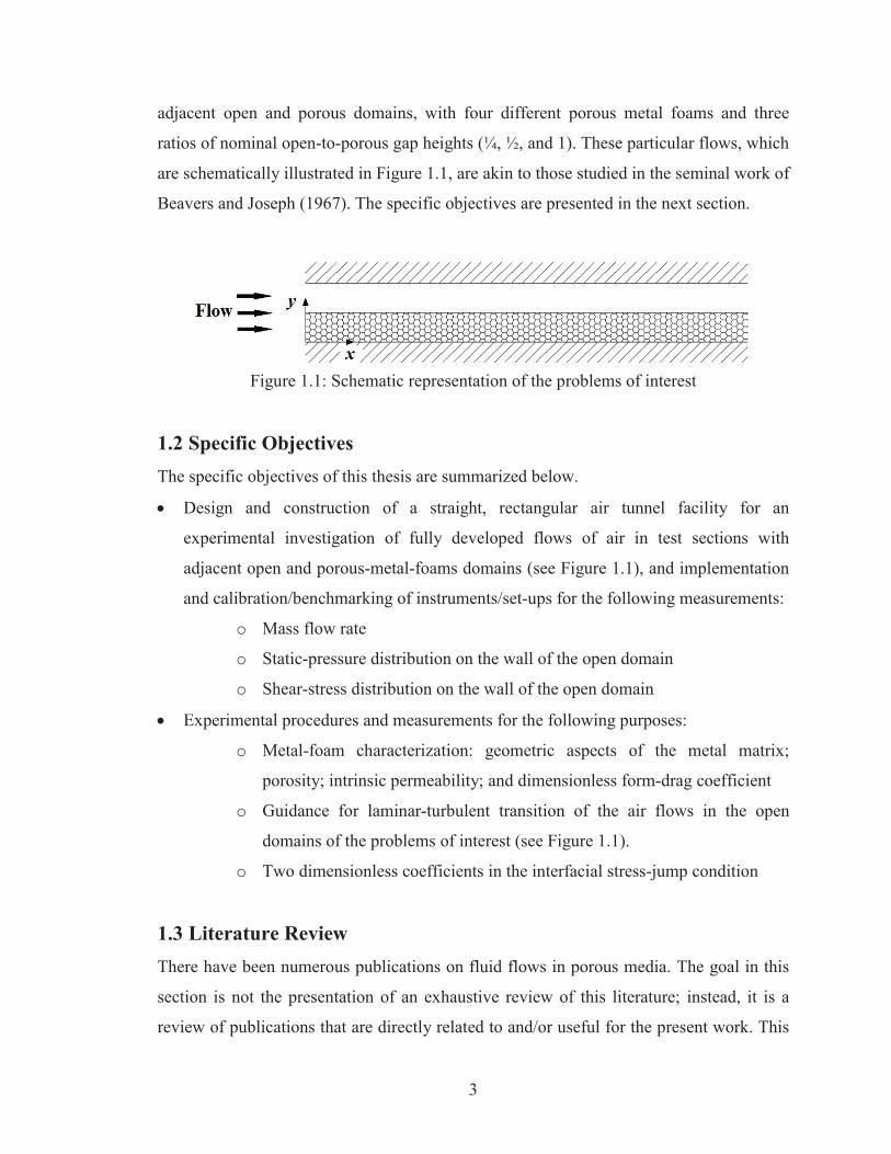
are schematically illustrated in Figure 1.1, are akin to those studied in the seminal work of
Beavers and Joseph (1967). The specific objectives are presented in the next section.
Figure 1.1: Schematic representation of the problems of interest
1.2 Specific Objectives The specific objectives of this thesis are summarized below.
Design and construction of a straight, rectangular air tunnel facility for an
experimental investigation of fully developed flows of air in test sections with
adjacent open and porous-metal-foams domains (see Figure 1.1), and implementation
and calibration/benchmarking of instruments/set-ups for the following measurements:
o Mass flow rate
o Static-pressure distribution on the wall of the open domain
o Shear-stress distribution on the wall of the open domain
Experimental procedures and measurements for the following purposes:
o Metal-foam characterization: geometric aspects of the metal matrix;
porosity; intrinsic permeability; and dimensionless form-drag coefficient
o Guidance for laminar-turbulent transition of the air flows in the open
domains of the problems of interest (see Figure 1.1).
o Two dimensionless coefficients in the interfacial stress-jump condition
1.3 Literature Review There have been numerous publications on fluid flows in porous media. The goal in this
section is not the presentation of an exhaustive review of this literature; instead, it is a
review of publications that are directly related to and/or useful for the present work. This
4
review is subdivided into the following sections: (a) fluid flows and pressure drops in
porous media; (b) determination of the intrinsic permeability and form-drag coefficient;
and (c) fluid flows in adjacent open and porous domains.
1.3.1 Fluid Flows and Pressure Drops in Porous Media The seminal work in the area of fluid flows in porous media is attributed to Henry Darcy
(1856). Commissioned by the city of Dijon, a portion of his experiments dealt with water
filtration and led to the development of a relationship that is today referred to as “Darcy’s
Law” or the Darcy equation [Nield and Bejan (2013)]. This equation represents Darcy’s
finding that for steady-state, unidirectional, creeping, isothermal flow of an
incompressible Newtonian fluid (water) in an isotropic porous medium (filter), the ratio
of the average cross-sectional fluid velocity (superficial velocity) to the gradient of the
intrinsic phase-averaged pressure is equal to a constant value, k , dependent on both the
geometry of the porous medium and the fluid under consideration [Lage (1998)].
The current form of the Darcy equation incorporates a slight, but important, modification:
k , is replaced by the dynamic viscosity of the fluid divided by a different constant, K ,
denoted as the intrinsic permeability (from this point on, referred to as permeability),
which is independent of the fluid but dependent on the geometry of the porous medium
[Kaviany (1995); Dullien (1992); Nield and Bejan (2006)]. Lage (1998) calls it the
Hazen-Darcy equation (referred to in this thesis as the Darcy equation), and
acknowledges the related works of Hazen (1893) and Krüger (1918).
At fluid velocities greater than those involved in the study conducted by Darcy, Dupuit
(1863), borrowing ideas from Prony (1804), reasoned that the gradient of the intrinsic-
phase-averaged pressure could be calculated from a quadratic function of the superficial
velocity. The quadratic term was the drag (or “forme force”) the fluid experiences as it
flows past the solid obstacles within the porous medium [Lage (1998)]. The resulting
equation is commonly referred to as the Darcy-Forchheimer equation [Beavers et al.
(1973); Givler and Altobelli (1994); Nield and Bejan (2013)]; however, Lage (1998) has
5
called it the Hazen-Darcy-Dupuit equation, as Forchheimer (1901) had not proposed the
aforementioned extension, but only affirmed it.
Ward (1964) performed a dimensional analysis of the Darcy-Forchheimer equation, and
expressed the quadratic term as a product of the fluid density, square of the superficial
velocity, and a dimensionless form-drag coefficient, Fc , divided by the square root of the
permeability. Several different porous media made of particles that were approximately
spherical in shape were considered in the study by Ward (1964). The Fanning friction
factor for these porous media was plotted against a Reynolds number, based on the
permeability of the porous media. These plots demonstrated an asymptotic region at high
Reynolds numbers, in which the friction factor was effectively constant, leading him to
claim that the aforementioned drag coefficient was “universal” for all porous media.
Many authors have used the dimensionless form-drag coefficient divided by the square
root of the permeability as a dimensional form of this coefficient, C, [Lage (1998);
Boosma and Poulikakos (2003); Despois and Mortensen (2004)]. Some authors have
referred to the dimensional form-drag coefficient as a non-Darcian permeability
[Innocentini et al. (1999a, 1999b, 1999c); Moreira et al. (2004); Biasetto et al. (2007)].
Joseph et al. (1982) confirmed the usefulness of the dimensionless form-drag coefficient,
but with reference to the works of Beavers and Sparrow (1969) and Schwartz and
Probstein (1969), disagreed that it is a universal constant for all porous media.
A cubic term has been proposed as an extension to the Darcy-Forchheimer equation [Mei
and Auriault (1991); Firdaouss et al. (1997); Wodie and Levy (1991); Lage et al. (1997)].
However, Lage and Antohe (2000) claimed there is no experimental support (or physical
justification) for the inclusion of a cubic term. For flows in highly porous media,
Brinkman (1949) added an additional term, analogous to the viscous term found in the
Navier-Stokes equations, to account for the viscous shear stress on the fluid caused by the
surfaces within the porous medium. This term incorporates the so-called Brinkman or
effective dynamic viscosity of the fluid. It allows boundary-layer development along
interfaces (such as those adjacent to open domains and solid walls) and enables the
6
inclusion of suitable boundary conditions, such as the no-slip condition at boundary walls
[Givler and Altobelli (1994); Nield and Bejan (2013)]. Joseph et al (1982) recommend the
use of the dynamic viscosity of the fluid, and Vafai and Tien (1981) use the dynamic
viscosity of the fluid divided by the porosity, in place of the effective dynamic viscosity.
Further discussions of the Brinkman term can be found in Nield and Bejan (2013).
1.3.2 Determination of the Permeability and Form-Drag Coefficient If full details of the geometry of the porous medium are known, the permeability and
dimensionless form-drag coefficient can be determined theoretically [Dullien (1992);
Kaviany (1995); Nield and Bejan (2013)]. Thus, for fluid flows in beds of spherical
particles, both the permeability and dimensionless form-drag coefficient can be calculated
as functions of the porosity and mean particle diameter [Ergun (1952)]. For a close-
packed bed of spherical particles of the same diameter, the permeability can be calculated
using the Carman-Kozeny relationship [Nield and Bejan (2013)]. Additional expressions
of this type can be found in Dullien (1992).
For fluid flows in porous metal foams, some authors have proposed both empirical and
semi-empirical models to predict the permeability and form-drag coefficient. Edouard et
al. (2008) critically reviewed many proposed models based on a variety of geometric
properties, such as the pore diameter or window size, cell size, strut or ligament diameter,
porosity, number of pores per inch (PPI), specific surface area, and tortuosity. Purely
empirical models were not recommended due to the large experimental errors commonly
found in the related pressure-drop and velocity data available in the published literature.
Semi-empirical models were preferred, namely, those of du Plessis et al. (1994) and
Lacroix et al. (2007), as these models gave the best predictions ( 30%) of the
experimental data collected in the work of Edouard et al. (2008). In the study of du
Plessis et al. (1994) the pore diameter was calculated from the PPI designation provided
by the manufacturer. However, the PPI designation has been found to be an inaccurate
way of specifying or measuring the pore diameter [Onstad et al. (2012)].
7
Fourie and du Plessis (2002) built on the work of du Plessis (1994) and modeled the
porous-metal-foam structure with tetrakaidecahedrons. Using the analogy of a cylinder in
cross-flow to model the hydrodynamic stresses and recirculation in the metal foams at
higher Reynolds numbers, an equivalent cylinder diameter and representative hydraulic
diameter (RHD) were calculated. The permeability was calculated solely as a function of
cell diameter, porosity, and tortuosity, whereas the dimensionless form-drag coefficient
was also calculated as a function of the Reynolds number. Woudberg and du Plessis
(2010) further refined the model of du Plessis et al. (1994), to make it applicable to high-
porosity foams. Lacroix et al. (2007) used silicon carbide foams and modeled the foam
structure as a dodecahedron cell. In the equations they put forth, the cell size (diameter of
the dodecahedron) of the foam was the only parameter required for determining the
permeability and form-drag coefficient. The authors stated they cannot give any physical
reasoning to explain their model, but it predicted their experimental data well.
Calmidi (1998) represented the structure of high-porosity metal foams by dodecahedron-
shaped cells, and then related the parameters of the dodecahedron cell to a unit-cube-cell
made from cylindrical rods. The porosity and cell size of the foam (distance between two
pentagonal faces of the dodecahedron) were used as inputs to a semi-empirical correlation
for the determination of the permeability and form-drag coefficient. Also incorporated
into the proposed semi-empirical correlation was the ratio of ligament diameter to pore
diameter of the dodecahedral cell, which included a shape factor to account for the
change in ligament cross-section, which was observed to be a function of the porosity.
When using the aforementioned or any other empirical or semi-empirical models found in
the literature for the determination of the permeability and dimensionless form-drag
coefficient, it should be noted that there are many discrepancies in the available
experimental results: for example, pressure-drop data for metal foams available in the
literature are inconsistent [Paek et al. (2000); Moreira et al. (2004)]. These discrepancies
can be attributed to inadequacies in experimental procedures and analyses for determining
the permeability and dimensionless form-drag coefficient. There are also inconsistencies
and difficulties in the methods for determining the microstructure of the foam [Paek et al.
8
(2000); Madani et al. (2007)]. These, in turn, have adverse effects on the accuracy of
related semi-empirical models.
Semi-empirical models are desirable from a practical standpoint, but not when large
errors, such as those encountered in Edouard et al. (2008), are unacceptable. For a
potentially more accurate approach, reliable experimental pressure-drop and superficial-
velocity data are required from investigations of steady-state, unidirectional,
incompressible flow of a Newtonian fluid in porous media with negligible boundary
effects. Under these assumptions, the Darcy-Forchheimer equation is applicable, and the
permeability and form-drag coefficient can be calculated by performing a least-squares
curve-fit of the experimental data [Ward (1964); Beavers et al (1973); Givler and
Altobelli (1994); Antohe et al. (1997); Calmidi (1998); Innocentini et al. (1999a, 1999b,
1999c); Boosma and Poulikakos (2002); Zeng and Grigg (2006); Biasetto et al. (2007)].
Dukhan and Minjeur II (2011) proposed that two permeabilities exist, one for fluid flow
within the Darcy regime, and another in the Forchheimer regime, referred to as the
Darcian and Forchheimer permeabilities, respectively. Miwa and Revankar (2009)
performed experiments, only collecting data in the Darcy regime, and subsequently
calculated the permeability of the metal foam (INCO) used in their study. The data of
Innocentini et al. (1999a) appeared to be within the Darcy regime, and the form-drag
contributed as low as one percent of the total pressure drop, but no comparisons similar to
those undertaken by Ward (1964) were made. Investigations akin to that of Dukhan and
Minjeur II (2011) require demarcation of the conditions when the fluid flow transitions
from the Darcy regime to the quadratic Forchheimer regime. Boosma and Poulikakos
(2002) calculated the permeability from data points within the Darcy regime and
determined a transitional (from Darcy to Forchheimer regimes) Reynolds number based
on the permeability. They maintained that all data points should be used for the
determination of the permeability and form-drag coefficient.
Flow transition from Darcy to Forchheimer regimes has primarily been tied to values of
the superficial velocity, Reynolds number (with a variety of parameters used as the length
9
scale), and Forchheimer number. Biasetto et al. (2007) have suggested a transitional
superficial velocity of 0.1 m/s. Bonnet et al. (2008) used the pore diameter as a length
scale and determined a transitional Reynolds number to be approximately 200. Miwa and
Revankar (2009) stated that the pore diameter is an inappropriate length scale, as it varies
widely in porous metal foams. They and other authors suggested that a more appropriate
length scale is the square-root of the permeability. Givler and Altobelli (1994) and Lage
et al. (1997) concluded that such a transition occurs at a permeability-based Reynolds
number of unity, while Boosma and Poulikakos (2002), Boosma et al. (2003), and Miwa
and Revankar (2009) proposed values of 10, 20, and 26.5, respectively.
Lage (1998) argued that a good indicator of the transition from Darcy to Forchheimer
regimes is the ratio of form-drag to viscous-drag forces, often referred to as the
Forchheimer number; this ratio could also be considered as a Reynolds number with the
product of the permeability and dimensional form-drag coefficient as the length scale.
Lage et al. (2005) and Zeng and Grigg (2006) reported critical Forchheimer numbers of
unity and 0.11, respectively. The critical value proposed by Zeng and Grigg (2006) was
determined from a more practical point of view, based on their finding that the
aforementioned transition occurs when the form-drag term of the Darcy-Forchheimer
equation accounts for ten percent of the overall pressure drop. Innocentini et al. (2010)
reported that a Forchheimer number much less than unity ensures that the fluid flow is in
the Darcy regime. The square-root of the permeability and the pore diameter are the
primary length scales used in Reynolds numbers associated with high-porosity porous
metal foams. Lacroix et al. (2007), Madani et al. (2007), and Edouard et al. (2008) all
concluded that the strut or ligament diameter is the most suitable characteristic length
scale of the foam microstructure, but no Reynolds number based on ligament diameter
was found in the literature.
Determination of the permeability and form-drag coefficient from curve-fitting
experimental data requires special care to be taken with regard to the assumptions made
in modeling the flow with the Darcy-Forchheimer equation, namely, unidirectional,
incompressible, steady-state flow in an isotropic porous medium with negligible
10
boundary effects. Bonnet et al. (2008) stated that for a porous foam to be considered
homogenous, a minimum of ten pores must span each direction of the sample. They also
investigated the compressibility effects of air flowing in porous metal foams and recast
the Darcy-Forchheimer equation in terms of the gradient of the product of fluid density
and pressure, as function of the mass-flux density of the fluid, in lieu of the superficial
velocity. Many authors have used relatively thin foam samples and measured pressure
gradients from two-point measurements (at the inlet and the exit of the sample). Bonnet et
al. (2008) concluded that the behavior of the flow could not be properly characterized
under these conditions. Very few authors have measured pressure distribution profiles in
this context: those found in the literature included Beavers et al. (1973), Calmidi (1998),
Zhao et al. (2001), Madani et al. (2007), and Bonnet and Topin (2008).
When assuming steady-state flow, it is important that the measured pressure profiles
allow for the exclusion of non-steady entrance and exit effects from the calculation of the
pressure gradient. Madani et al. (2007) found the pressure gradients in the entrance and
exit regions to be higher than that in the fully developed region. Dukhan and Patel (2011)
investigated the influence of the total axial length of a foam sample on the calculated
values of the permeability and dimensionless form-drag coefficient. Foam-sample lengths
greater than 100 cell diameters ensured that the values of these parameters were
independent of the aforementioned influence. It should be noted that two-point pressure-
drop data were collected, thus the above-mentioned requirement on the sample length
also ensures that the entrance and exit effects on the pressure drop are minimized.
Innocentini et al. (2010) investigated the effect of the length of the sample and how it is
held when measuring the permeability. For highly-porous metal foams, the relative size of
the sample and holder should be selected appropriately, to eliminate the presence of
stagnant fluid zones and reduce the amount of radial diffusion of the fluid and
underestimation of the pressure drop across the sample.
Lage et al. (2005) proposed a procedure to evaluate the permeability and dimensionless
form-drag coefficient, by independently determining each term through the minimization
of the pressure-drop contribution of the other. When calculating the permeability, the
11
viscous effect of the bounding wall of the porous medium is also isolated and subtracted
from the pressure gradient. However, this study never stated a requirement on the height
of the porous medium, transverse to the axial flow direction, between the two bounding
walls of a rectangular or parallel-plate channel.
Dukhan and Ali (2012) determined a minimum-value requirement on the diameter of a
porous-metal-foam sample, to minimize the boundary effects of the containing tube wall,
in experiments for determining the permeability and form-drag coefficient. These
boundary effects were minimized for sample diameters greater than or equal to 63.5 mm,
equating to an approximate requirement of 15 and 30 cell diameters for the 10 PPI and 20
PPI foam samples, respectively. Of note, all fourteen ERG Aerospace aluminum foam
samples used in their study were six inches long; and none of these samples met the
minimum requirement for length set forth in a previous study by one of the authors
[Dukhan and Patel (2011)]. Beavers et al. (1973) performed a similar experiment for beds
of randomly packed spheres. The permeability and form-drag coefficient were unaffected
when the equivalent hydraulic diameters of the bed were 12 times and 40 times the
diameter of the spherical particles, respectively.
1.3.3 Fluid Flows in Adjacent Open and Porous Domains The modeling of steady flows of incompressible Newtonian fluids in adjacent open and
porous domains can be segregated into three basic levels of description: microscopic,
mesoscopic, and macroscopic. The microscopic-scale description is an exact approach, in
which the fluid flows in both the open and porous domains are modeled by the continuity
and Navier-Stokes equations, and the no-slip boundary condition is applied at all fluid-
solid boundaries. However, this approach requires an exact description of the topology of
the porous medium, which poses a variety of difficulties for porous metal foams, such as
the high local heterogeneity [Chandesris and Jamet (2007)]. The storage capacity and
computer speed of modern computers also limits this approach, as numerical simulations
at this level of complexity would require too much time to be of any practical use. The
mesoscopic-scale description is a volume-averaged approach that treats the open and
porous regions as one single solution domain with one set of continuity and momentum
12
equations to describe the fluid flow [Goyeau et al. (2003), Chandesris and Jamet (2006,
2007, 2009), Jamet and Chandesris (2009), and Jamet et al. (2009)]. This approach
requires a heterogeneous transition zone to be defined in the vicinity of the interface
between the open and porous domains. As outlined in Costa et al. (2008), the difficulty in
this method is related to the description of such a transition zone, as it is nearly
impossible to accurately (or reliably) describe the strong variations in the effective
properties of the porous medium in this region. In the macroscopic-scale description, the
open and porous regions are treated as two separate solution domains, each with their
own set of governing equations. To couple the two domains, a suitable boundary
condition is imposed at their interface. This approach is the most useful one for modeling
practical problems, but it does have some difficulties related to the assigning of suitable
values to the coefficients that are involved in the interfacial boundary condition
[Chandesris and Jamet (2007)].
As the macroscopic-scale description is the most practical approach to modeling
Newtonian fluid flows in adjacent open and porous domains, the remainder of this section
is focused on the various interfacial boundary conditions available in the literature, as
well as attempts at determining the various coefficients that arise in such conditions. The
discussions will be limited to laminar fluid flows. For discussions on the modeling of
turbulent fluid flows in adjacent open and porous domains, and the related approaches
and challenges, the reader is referred to the works of Prinos et al. (2003), de Lemos and
Silva (2006), McLean and Nikora (2006), Breugem et al. (2006), Chan et al. (2007),
Finnigan and Shaw (2008), Saito and de Lemos (2010), Suga et al. (2010, 2011),
Higashino and Stefan (2012), and de Lemos (2012).
Beavers and Joseph (1967) provided the seminal experimental and numerical research
work in this area. They investigated steady Newtonian fluid flows in a uniform parallel-
plate channel that was partially occupied by naturally homogenous and isotropic
permeable blocks; these blocks were made from aloxite or metal foam (FOAMETAL).
The flows in the adjacent open and porous domains were modeled using the continuity
and Navier-Stokes, and the Darcy equation, respectively. The pressure and the normal
13
component of the fluid velocity were assumed to be continuous at the interface. Darcy
flow was assumed, with a uniform superficial velocity prevailing in the entire porous
domain up to the interface. To account for the observed boundary layer within the porous
domain, a slip condition with one adjustable dimensionless coefficient was proposed to
relate the velocity gradient in the open-domain side, evaluated at the interface, to the
open-domain fluid velocity at the interface and the superficial velocity in the porous
block. With the experimental data collected, the adjustable coefficient in the imposed slip
condition was determined for each of the porous blocks. It was found that this
dimensionless coefficient depends strongly on the exact location of the interface,
properties of the porous medium, and the type of flow regime encountered [Kaviany
(1995), Goyeau et al. (2003), Chandesris (2006, 2007)].
Neale and Nader (1974) modeled the flow in the open domain using the continuity and
Navier-Stokes equations, and the Brinkman-extended Darcy equation for the flow within
the porous domain. The velocity and also the normal and tangential components of the
stress, based on the dynamic viscosity of the fluid in the open domain and an effective
viscosity in the porous domain, were assumed to be continuous at the interface. They
argued that the Brinkman term would implicitly resolve the boundary layer within the
porous medium and remove the necessity of the velocity slip condition. Their solution
matched that of Beavers and Joseph (1967), and it also had the advantage of describing
the boundary layer within the porous domain. By comparing the two solutions, the
coefficient in the slip condition of Beavers and Joseph (1967) was found to be equal to
the square-root of the ratio of the effective dynamic viscosity to dynamic viscosity of the
fluid. The difficulty involved with the model proposed by Neale and Nader (1974) is
related to the determination of a suitable effective dynamic viscosity.
Vafai and Kim (1990) presented an analytical solution to the problems of interest,
modeling the fluid flow in the open domain using the continuity and Navier-Stokes
equations, and the Brinkman-Darcy-Forchheimer equation for the fluid flow within the
porous domain. The effective dynamic viscosity was assumed to be equal to the dynamic
viscosity of the fluid, and the velocities and the gradients of the velocity in the open and
14
porous domains were assumed to be continuous at the interface. They also discussed how
the velocity profile was affected by changes in the Darcy number and product of the
Reynolds number with a specially defined inertial parameter.
Ochoa-Tapia and Whitaker (1995a) modeled the flow in the open domain with the
continuity and Stokes equations, and the extended Brinkman-Darcy equation in the
porous domain, with the effective dynamic viscosity equal to the dynamic viscosity of the
fluid divided by the porosity. They proposed a continuous velocity field at the interface
and an interfacial tangential stress-jump condition, based on the excess viscous stress at
the interface, which involved one dimensionless adjustable coefficient of order unity. In
the second part of their study, Ochoa-Tapia and Whitaker (1995b) compared their
theoretical model to the experimental data of Beavers and Joseph (1967) for the
determination the aforementioned dimensionless coefficient. A variable-porosity model
of the interface region was also investigated, as an alternative to the stress-jump
condition, but it did not produce results that matched the experimental data. Although
they successfully determined that the adjustable dimensionless coefficient is of order one,
they could not deduce an empirical relationship for this coefficient. Ochoa-Tapia and
Whitaker (1998) included inertial terms in their derivations. The continuity and Navier-
Stokes equations were used to model the fluid flow in the open domain, and the
Brinkman-Darcy-Forchheimer equation was employed to model the fluid flow in the
porous domain. The interfacial stress-jump boundary condition was revisited, and an
additional term was added to account for the excess inertial stress; it too contained a
dimensionless adjustable coefficient of order one or less. In both studies, it was stated that
experimental data should be used to determine these dimensionless coefficients.
Alazmi and Vafai (2001) discussed four interfacial heat-transfer conditions, and five of
the aforementioned interfacial boundary conditions for fluid flows in adjacent open and
porous domains. They compared and contrasted the effects of modifying a variety of
parameters, namely, the Darcy number, an inertia parameter, Reynolds number, porosity,
effective viscosity, and slip coefficients, on the velocity field, temperature field, and
Nusselt number distribution. It was found that the effects of varying these parameters had
15
a much greater effect on the velocity field than on either the temperature field or Nusselt
number distribution. Changing the effective dynamic viscosity from the dynamic
viscosity of the fluid to a recommended value given by Givler and Altobelli (1994) had a
relatively minimal effect on the velocity field, given that the range of values for the
effective dynamic viscosity was quite wide. Following the analysis of Vafai and Tien
(1981), the authors recommended that the effective dynamic viscosity be set equal to the
dynamic viscosity of the fluid divided by the porosity.
Deng and Martinez (2005) also expressed the need for accurate determination of the
dimensionless coefficient found in the interfacial conditions, to obtain meaningful
solutions to the problems of interest. They used two different approaches to obtain an
estimate of the value of the dimensionless coefficient in the stress-jump condition of
Ochoa-Tapia and Whitaker (1995a). One was the two-domain macroscopic approach with
the continuity and Navier-Stokes equations in the open domain, the extended Brinkman-
Darcy equation in the porous domain, and the interfacial boundary condition of Ochoa-
Tapia and Whitaker (1995a). In the second approach, a single-domain model was used.
With each solution producing similar results, the dimensionless coefficient was estimated
using a curve-fitting method. It was found that this coefficient was a function of the
Reynolds number and the Darcy number, and it was of order one.
Kuznetsov (1997, 1999) extended the analytical approach provided in Vafai and Kim
(1990) by incorporating the stress-jump condition of Ochoa-Tapia and Whitaker (1995a),
and an effective dynamic viscosity, rather than using the continuity of the gradient of the
velocity as an interfacial boundary condition. His analytical solution included the
effective dynamic viscosity, and it was demonstrated that the selection of the value of this
term, as well as the value of the stress-jump coefficient, could affect the velocity profile.
This effect was also found to decrease with an increase in the inertial parameter, and
decrease in Darcy number.
Costa et al. (2008) numerically investigated laminar fluid flows in the problems of
interest. They modeled the fluid flow in the open domain with the continuity and Navier-
16
Stokes equations, the fluid flow in the porous domain with the Brinkman-Darcy-
Forchheimer equation, and the interfacial boundary condition with the stress-jump
condition of Ochoa-Tapia and Whitaker (1998). The mathematical model was solved with
a control-volume finite-element method (CVFEM), and they proposed a novel procedure
to implement the stress-jump condition. To validate their procedure, they compared their
results with an adapted version of the analytical solution of Kuznetsov (1999) to include
the second coefficient in the tangential stress-jump condition. The values of the two
adjustable coefficients in the tangential stress-jump condition were varied, and their effect
on the flow field was found to be significant. They concluded that for accurate numerical
predictions, experimental data is required to determine these stress-jump coefficients.
A number of numerical investigations have been devoted to the evaluation of the
aforementioned coefficients in the interfacial boundary conditions. Nabovati and Sousa
(2007) used the lattice-Boltzmann method to investigate the flow characteristics at the
interface, demonstrated that the Beavers and Joseph (1967) slip coefficient was a function
of porosity, and proposed an equation to model this slip coefficient. Valdés-Parada et al.
(2009) derived an analytical expression for the coefficient in the stress-jump condition put
forward by Ochoa-Tapia and Whitaker (1995a), by combining ideas borrowed from the
analyses of Goyeau et al. (2003) and Valdés-Parada et al. (2007).
Other than the seminal work of Beavers and Joseph (1967), there have been only a few
experimental studies of fluid flows in adjacent open and porous domains. Beavers et al.
(1970) performed an experimental investigation and collected pressure-drop data for
laminar and turbulent fluid flows in a parallel-plate channel that contained adjacent open
and porous-metal-foam domains (FOAMETAL). Their data validated the use of a
velocity-slip model and indicated that the metal foam delayed the laminar-to-turbulent
transition in the open domain, as determined from flow visualizations. The transitional
Reynolds number, based on the hydraulic diameter of the parallel-plate channel, was
found to be between 2765 and 3150.
17
Prinos et al. (2003) have experimentally (and also numerically) studied the characteristics
of the turbulent flow of water in open channels with a porous bed. The porous bed was
made up of a bundle of cylindrical rods, and their diameter and spacing were adjusted to
achieve values of permeability ranging from 5.5490 x 10⁻⁷ m2 to 4.1070 x 10⁻⁴ m2 and
porosity values from 0.4404 to 0.8286. Hot-film anemometry was used for measuring
mean velocities and turbulent stresses in the channel, with a bed-porosity value of 0.8286.
Emphasis was put on determining the effect the Darcy number had on the flow properties
over and within the porous region. The velocities in the open domain were found to
decrease with increasing values of Darcy number, due to the strong momentum exchange
near the open-porous interface and the corresponding penetration of turbulence into the
porous layer for highly permeable beds.
Arthur et al. (2009) took particle-image velocimetry (PIV) measurements to investigate
the velocity profile of pressure-driven fluid flows in various models of porous media.
Installed in a rectangular channel, the porous medium consisted of arrays of circular
acrylic rods, positioned to create porosities ranging from 0.01 to 0.49. One of the models
investigated involved flows with an open domain above the rods. The velocity profile
near the interface was fitted with a fourth-order least-squares curve fit, and the gradient of
the velocity was found from differentiating this curve fit. Such measurements could be
used for validating the results of corresponding numerical predictions and determining the
coefficients in the interfacial boundary condition.
Carotenuto et al. (2012) induced a shear-driven flow above and below a porous medium
via a rotational rheometer to mimic a parallel-plate configuration. Sand papers of two
different grits were used and considered as very thin porous media. Shear-induced flow
above the porous medium allowed for determination of the velocity profile in the open
domain as well as the fluid velocity at the interface. Flow induced from below directly
determined the stress transferred through the porous layer to the fluid in the open domain,
as well as the fluid velocity in the porous layer. For the finer-grit sandpaper, it was found
that the stress transferred to the fluid within the open domain was smaller than the applied
stress, but this difference was within the experimental error bounds.
18
With the relative dearth of experimental studies of fluid flow in adjacent open and porous
domains, there is an explicit need for accurate measurements of data required for
determining the two adjustable coefficients in the tangential stress-jump condition of
Ochoa-Tapia and Whitaker (1998), and also for the checking and refining numerical
simulations of such fluid flows. This need is even more urgent for flows in adjacent open
and porous-metal-foam domains, as there appear to be no experimental studies of such
flows in the published literature, except for the work of Beavers and Joseph (1967) and
Beavers et al. (1970) to the best knowledge of the author.
1.4 Organization of the Thesis In the earlier sections of this chapter (Chapter 1), the motivation and overall goals,
specific objectives, and a literature review on topics relevant to this research were
presented. In Chapter 2, the theoretical considerations that were used for designing the
experimental set-ups and procedures, implementing (selecting, calibrating, and
benchmarking) related instrumentation, and processing the experimental measurements
are presented and discussed. Descriptions of the experimental apparatus and procedures
proposed and used in this work are given in Chapter 3. In Chapter 4, the results are
presented and discussed. Chapter 5 concludes the main body of this thesis, and contains a
review of the thesis, a summary of the main contributions of this work, and also
recommendations for extensions of this work.
19
Chapter 2 – Theoretical Considerations
As was stated in Chapter 1, the focus of the work reported in this thesis was on
experimental investigations of Newtonian fluid flows through straight rectangular ducts,
with cross-sections of large aspect ratio (so the central regions of these ducts are akin to a
parallel-plate channel) that were either entirely open (containing no porous medium),
completely filled with a porous medium, or contained adjacent open and porous domains
with a distinct interface parallel to the top and bottom walls. A longitudinal cross section
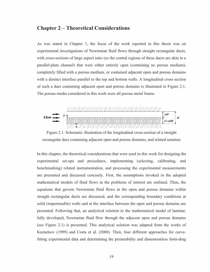
of such a duct containing adjacent open and porous domains is illustrated in Figure 2.1.
The porous media considered in this work were all porous metal foams.
Figure 2.1: Schematic illustration of the longitudinal cross-section of a straight
rectangular duct containing adjacent open and porous domains, and related notation
In this chapter, the theoretical considerations that were used in this work for designing the
experimental set-ups and procedures, implementing (selecting, calibrating, and
benchmarking) related instrumentation, and processing the experimental measurements
are presented and discussed concisely. First, the assumptions invoked in the adopted
mathematical models of fluid flows in the problems of interest are outlined. Then, the
equations that govern Newtonian fluid flows in the open and porous domains within
straight rectangular ducts are discussed, and the corresponding boundary conditions at
solid (impermeable) walls and at the interface between the open and porous domains are
presented. Following that, an analytical solution to the mathematical model of laminar,
fully developed, Newtonian fluid flow through the adjacent open and porous domains
(see Figure 2.1) is presented. This analytical solution was adapted from the works of
Kuznetsov (1999) and Costa et al. (2008). Then, four different approaches for curve-
fitting experimental data and determining the permeability and dimensionless form-drag
20
coefficient for flows through the porous metal foams are proposed and discussed. The
definitions of several pertinent friction factors are then presented, along with analytical
solutions (when possible) or empirical correlations (when available).
2.1 Assumptions The following assumptions were invoked in the adopted mathematical models of fluid
flows in adjacent and porous domains (see schematic in Figure 2.1):
The same Newtonian fluid saturates both the open and porous domains
Steady-state (statistically) conditions prevail
The fluid is incompressible and isothermal, thus, its mass density and dynamic
viscosity, evaluated at mean values of temperature and pressure in the region of
interest, are constants throughout the open and porous domains. Furthermore, fully
developed fluid flow prevails.
The open and porous domains are separated by a sharp interface parallel to the bottom
and top walls, and the location of this interface is known a priori
The porous medium (metal foams investigated in this work) is homogenous and
isotropic. In particular, the porosity and permeability of the porous metals foams are
uniform and constant throughout, from the bottom wall of the channel right up to the
interface between the open and porous domains.
2.2 Governing Equations and Boundary Conditions The full unsteady, three-dimensional equations that govern the Newtonian fluid (air)
flows considered in this work, in both the adjacent open and porous domains, are the
continuity and Navier-Stokes equations [Batchelor (1967); White (1991)]. As was
discussed in Section 1.3.3, the macroscopic approach is the most practical and effective
way of the modeling fluid flows in adjacent open and porous domains, and this approach
is adopted in this work. In this approach, the fluid flow in the open domain is modeled
using the above-mentioned the continuity and Navier-Stokes equations, and in the porous
domain, the volume-averaged forms of these equations are used.
21
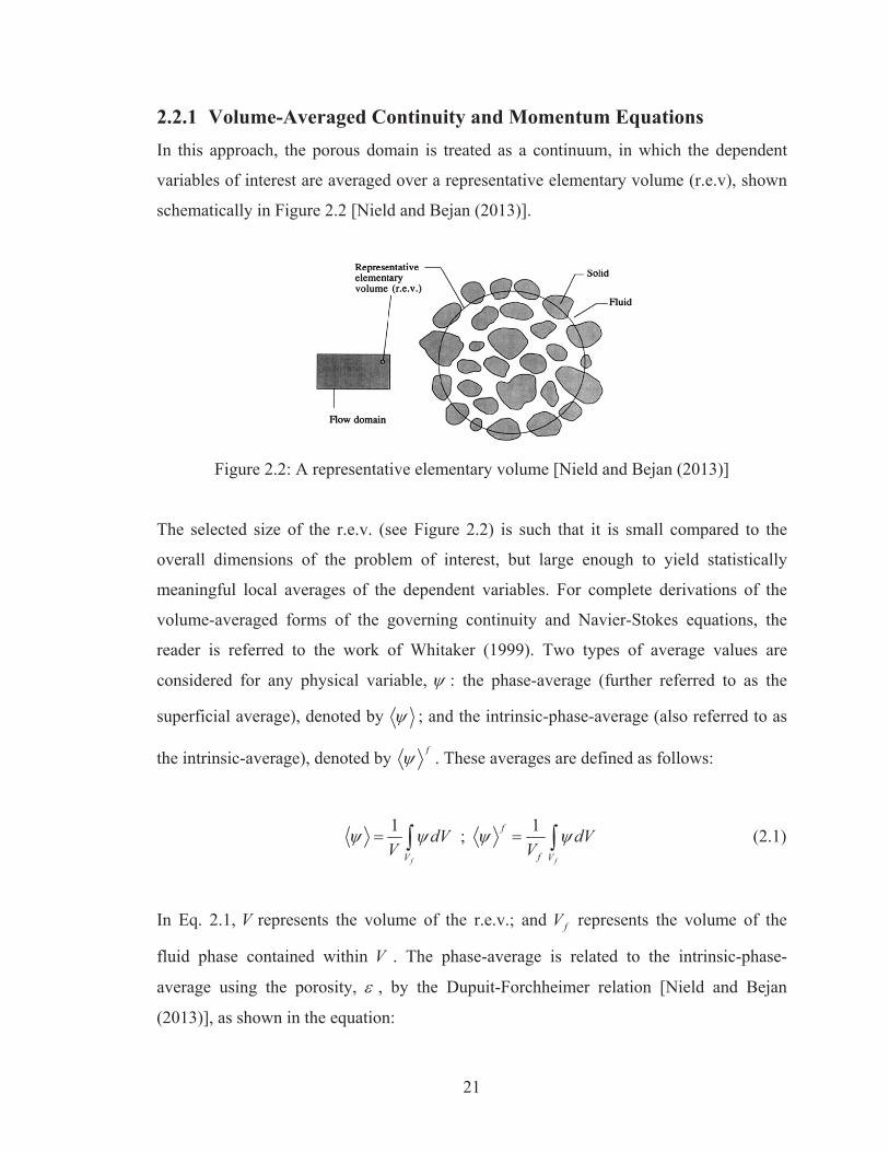
2.2.1 Volume-Averaged Continuity and Momentum Equations In this approach, the porous domain is treated as a continuum, in which the dependent
variables of interest are averaged over a representative elementary volume (r.e.v), shown
schematically in Figure 2.2 [Nield and Bejan (2013)].
Figure 2.2: A representative elementary volume [Nield and Bejan (2013)]
The selected size of the r.e.v. (see Figure 2.2) is such that it is small compared to the
overall dimensions of the problem of interest, but large enough to yield statistically
meaningful local averages of the dependent variables. For complete derivations of the
volume-averaged forms of the governing continuity and Navier-Stokes equations, the
reader is referred to the work of Whitaker (1999). Two types of average values are
considered for any physical variable, : the phase-average (further referred to as the
superficial average), denoted by ; and the intrinsic-phase-average (also referred to as
the intrinsic-average), denoted by f . These averages are defined as follows:
1 1;f f
f
fV V
dV dVV V
(2.1)
In Eq. 2.1, V represents the volume of the r.e.v.; and fV represents the volume of the
fluid phase contained within V . The phase-average is related to the intrinsic-phase-
average using the porosity, , by the Dupuit-Forchheimer relation [Nield and Bejan
(2013)], as shown in the equation:
22
; /ffV V (2.2)
Using Eq. 2.2, and invoking the assumption of constant fluid properties, the volume-
averaged continuity and the Navier-Stokes equations within the porous medium, in terms
of intrinsic-phase-average quantities, can be cast in the following forms, respectively:
0ii
ux
(2.3)
2
2 2
1 1 i Fi i j i
j i j
u cpu u u ut x x x K K
v (2.4)
In these equations, for simplicity of notation, the superficial velocity vector is denoted by
v , its components in the Cartesian coordinate directions are denoted by iu and ju , in the
i and j directions, respectively; p is used to denote the intrinsic-phase-average static
pressure of the fluid; is the density of the fluid; is the dynamic viscosity of the
fluid; K is the intrinsic permeability of the porous medium (hereafter referred to simply
as the permeability); and Fc is the dimensionless form-drag coefficient (also referred to
as the Forchheimer coefficient in the literature). It should be noted here that traditionally,
the / term was not used; rather, the so-called Brinkman dynamic viscosity of the
fluid, B , or effective dynamic viscosity of the fluid, eff , was used in its place [Nield
and Bejan (2013)], and it was thought that B needed to be determined from
experimental data. However, Whitaker (1999) did a rigorous derivation of the volume-
averaged equations, and showed that it was, indeed, correct to use / in the volume-
averaged momentum equations. It should also be noted that the time-derivative term in
Eq. 2.4 is zero under steady-state conditions.
2.2.2 Boundary Conditions at Solid Walls With respect to the schematic in Figure 2.1, at the inner surfaces of the bottom and top
walls of the duct, the no-slip and impermeability conditions apply:
23
1 2 3 1 2 3at 0, , , 0 ; and at , , , 0y u u u y H u u u (2.5)
2.3 Conditions at the Interface Between the Open and Porous Domains At the interface between the open and porous domains, the normal and tangential
components of the fluid velocity, the static pressure in the open domain and the intrinsic-
phase-average pressure in the porous domain, and the normal stresses in the open and
porous domains (indicated by the subscripts ‘od’ and ‘pd’, respectively) are assumed to
be continuous [Nield and Bejan (2013)], as expressed below in Eq. 2.6, with the total
stress tensor given by Eq. 2.7:
; ;I II I I I
j i ij j i ijod pd od pd od pdv v p p n n n n (2.6)
jiij ij
j i
uu px x
(2.7)
The notation used in Eqs. 2.6 and 2.7 is borrowed from Costa et al. (2008): the first-order
tensor in (or jn ) is a unit vector normal to the interface; ij is the Kronecker delta
function; the components of the total stress tensor, ij , in the open domain are calculated
from the static pressure and the components of the fluid velocity in the open domain,
whereas, in the porous domain they are calculated from the intrinsic-phase-average static
pressure and the components of the superficial velocity; and the superscript ‘I’ indicates
conditions at the interface between the open and porous domains.
Following the arguments put forward by Ochoa-Tapia and Whitaker (1998), if the
porosity, , and the permeability, K , of the porous medium are assumed to be uniform
throughout it, right up to the interface between the open and porous domains, then the
implied excess tangential stress at the interface has to be accounted for by the interfacial
condition presented in the following equation:
24
21 2
I It t
t tpd od
u u u un n K
(2.8)
In this equation, tu is the absolute value of the component of the fluid velocity tangential
to the interface; n is a local coordinate normal to the interface and points from the porous
domain to the open domain; and 1 and 2 are adjustable coefficients connected to the
implied excess viscous stress and the implied excess inertial stress, respectively, at the
interface. As is discussed in Ochoa-Tapia and Whitaker (1995b, 1998), the two adjustable
coefficients in the interfacial boundary condition expressed in Eq. 2.8 are of order unity
or less and are to be determined using experimental data.
2.4 Analytical Solution to the Problems of Interest for Laminar Flows The problems of interest (see Figure 2.1) are akin to that considered in the now classical
investigation of Beavers and Joseph (1967). In the experimental investigation, straight
rectangular ducts with cross-sections of high aspect ratio (Wchannel / H , where H is the
total height and channelW is the width of the duct cross-section) were used (related details
are provided in Chapter 3), and they contained the adjacent open and porous domains. In
the central portion of these rectangular ducts, because of the high-aspect ratio of their
cross section, the fluid flow was, for all practical purposes, similar to that in a parallel-
plate channel containing adjacent open and porous domains, akin to that illustrated in
Figure 2.1. Also shown in this figure is the following notation: H , H , and (1 )H
are the total, open-domain, and porous-domain heights; and is the ratio of the open-
domain height to the total-channel height.
An analytical solution can be now obtained by invoking the following assumptions, in
addition to those in Section 2.1 [Kuznetsov (1999); Costa et al. (2008)]:
The interface between the open and porous domains is flat and parallel to the top
and bottom walls of the channel
Fluid flow is steady and laminar
25
Fully developed flow prevails: thus, the velocity component in the y direction, v,
is zero; the velocity in the x direction, u, is invariant in this direction and is only a
function of the y coordinate; ( / )p y = 0 throughout the region of interest; and
( / )dp dx = constant.
Here, u and v are the actual velocity components in the open domain, and they represent
the corresponding components of the superficial velocity inside the porous domain; and
p is the actual static pressure in the open domain, and it denotes the intrinsic-phase-
average static pressure of the fluid inside the porous domain.
At this stage, H and U dp / dx H 2 / are taken as the reference length and
velocity, respectively, and the following dimensionless variables and parameters are
introduced, following Costa et al. (2008): u* u /U ; y* y / H ; Re UH / , which is
the Reynolds number based on U and H ; and Da K / H 2 , which is the Darcy number.
In the context of the assumptions introduced above and the aforementioned dimensionless
variables and parameters, the x-direction momentum equations in the open and porous
domains can be cast in the following dimensionless forms, respectively:
*
* *
0 1 duddy dy
(2.9)
***
* *
Re1 10 1 Fc udud udy dy DaDa
(2.10)
The dimensionless form of the stress-jump condition at the interface between the open
and porous domains is the following:
2* *1 * 2 *
* *
1 1 ReI I
pd od
du du u udy dy Da
(2.11)
26
In Eq. 2.11, *y is the dimensionless coordinate normal to the interface and points from
the porous domain to the open domain.
An analytical solution can be derived for the dimensionless velocity field, *u , by making
the following assumptions: two boundary layers exist within the porous domain, one
adjacent to the interface, located at * (1 )y , and the other one next to the bottom wall
of the channel, located at * 0y ; and these two boundary layers merge in the central
region of the porous domain, where du* / dy* 0 . With these assumptions, Eq. 2.10
reduces to a simple quadratic algebraic equation in the central portion of the porous
domain (where du* / dy* 0 ), and the positive root of this quadratic equation is the
solution for the dimensionless velocity in this region, * *u u :
2
*Re1 1 4 ;
2FcDa Fu F
DaF Da (2.12)
The dimensionless velocity field within the boundary layer near the bottom wall can now
be obtained by integrating Eq. 2.10 with respect to *y , subject to the following boundary
conditions: * 0u at * 0y ; and * *u u where the two boundary layers merge; and
noting that * */ 0du dy where the two boundary layers merge, *u can be determined.
This solution is represented by the following set of equations:
2
1* * 1* 1*
1
1* * 1 *
* 1*1 1*1
1 * 1*
11
32 ; exp2
21 ; ;1 3
zu u u uz
u u z A ByDaF
F u u uA Bu u
(2.13)
27
The dimensionless velocity field within the boundary layer adjacent to the interface can
be obtained by integrating Eq. 2.10 with respect to *y , subject to the following boundary
conditions: * *Iu u at * (1 )y ; and * *u u and du* / dy* 0 where the two
boundary layers merge. The solution is represented by the following set of equations:
2
2* * 1* 1*
2
2 * 1*2 * 2
2 1*
11
1exp 1 ; ;1
I
zu u u uz
u uz C B y Cu u
(2.14)
In the open domain, the solution for the dimensionless velocity field can be obtained by
integrating Eq. 2.9 with respect to *y , subject to the following boundary conditions:
* 0u at * 1y ; and * *Iu u at * (1 )y . The solution is the following:
2 ** * *0.5 1 0.5 1
Iuu y y (2.15)
In the experimental investigation undertaken in this work, values of the shear stress at the
upper wall of the open domain, odUW , located at y H , and the pressure gradient,
/dp dx , in the fully developed region were measured. Using these measurements, the
dimensions of the open and porous domains of the channel, and an overall force balance
on the open domain (from the interface between the open and porous domains to the inner
surface of the upper wall), the open-domain shear stress at the interface, Iod , can be
calculated using the following equation:
( / )I UWod oddp dx H (2.16)
It should be noted that this equation applies to not only laminar flows, but also turbulent
flows in a time-averaged sense.
28
Then, using the measured values of UWod , dp / dx , the dimensions of the open and porous
domains, and the calculated value of Iod , the following dimensionless quantities can be
calculated using Eqs. 2.12 to 2.15: the dimensionless velocity in the central region of the
porous domain, *u ; the dimensionless variable 1*u ; and the dimensionless quantities B
and C. After that, the following equations can be used to calculate the dimensionless
velocity at the interface, *Iu , and the dimensionless velocity gradients at the interface in
the open and porous domains, (du* / dy*)odI and (du* / dy*) pd
I , respectively:
u*I [0.5 2
odI /{( dp / dx)H}]
(du* / dy*)odI [0.5 (u*
I / )]
(du* / dy*) pdI 4(u * u1*)
(1 C)3 (1 C)CB
(2.17)
After the above-mentioned calculations, the terms interfaceY and interfaceX in the following
the dimensionless form of the interfacial stress-jump condition can be calculated:
* **
* *
2
* *
1 2
1 1
1Re
I II
interfacepd od
I Iinterface
interface interface
du duY udy dy Da
X u uDa
Y X
(2.18)
Thus, from each set of experimental measurements corresponding to laminar flow in the
channel with adjacent open and porous domains, the corresponding set of terms interfaceY
and interfaceX in Eq. 2.18 can be obtained. Then, a least-squares linear-curve-fit to these
pairs of terms ( interfaceY and interfaceX ) can be done, and the intercept and the slope of this
linear-curve-fit gives the stress-jump coefficients 1 and 2 .
29
2.5 Determination of the Permeability and Form-Drag Coefficient The permeability and dimensionless form-drag coefficient are two parameters that are
critically important for modeling fluid flow through a porous medium. As was discussed
in Section 1.3.2, a number of semi-empirical correlations for determining these two
parameters for porous metal foams akin to the ones used in the present work are available
in the literature. Although such semi-empirical correlations are desirable from a practical
point of view, they are usually not generally applicable, even for the same batch of porous
metal foams. The reason for this lack of generality is that porous metal foams with the
same nominal PPI designation and bulk density, and made by the same manufacturer, can
have significantly different geometric characteristics, due to inevitable differences
incurred in the foam topology during the manufacturing process [Moreira et al. (2004);
Edouard et al. (2008)].
Thus, whenever possible, the permeability and dimensionless form-drag coefficient
should be determined experimentally, directly with the porous metal foam to be used in
the application of interest or with a sample cut from this particular metal foam. This is the
approach that was adopted in this work. The specific experimental set-up involved
measurements related to fully developed Newtonian fluid flow in a straight rectangular
duct with a high-aspect-ratio cross-section filled completely with the porous metal foam
of interest, in a set-up that was akin to that illustrated schematically in Figure 2.1, but
with = 0. With this set-up, the following assumptions were invoked:
The porous metal foam is homogenous and isotropic
The Newtonian fluid saturates the entire porous metal foam that is filled inside the
rectangular duct
Steady-state (statistically) conditions prevail
The fluid is incompressible and isothermal, thus, its mass density and dynamic
viscosity, evaluated at mean values of temperature and pressure in the region of
interest, are constants throughout the open and porous domains.
The pressure drop in the fluid flow is caused primarily by the effects of the Darcy and
Forchheimer terms within the porous medium; or, in other words, the contributions of
30
the Brinkman term (within the porous medium and also at the walls of the duct) to this
pressure drop are negligibly small
The fluid flow is fully developed and one-dimensional in the region where the
measurements are made
With the above-mentioned assumptions, Eq. 2.4 reduces to the following simple form:
2Fcdp u udx K K
(2.19)
In Eq. 2.19, u denotes the superficial velocity and it is effectively constant in the region
of interest (equal to the average value of the superficial velocity in the rectangular duct, in
the region where the experimental measurements are made); and dp / dx is the axial
gradient of the pressure, and it too is constant in the region of interest. Thus, with
experimental data for u and dp / dx , and also the corresponding values of and , the
values of the permeability, K , and dimensionless form-drag coefficient, Fc , can be
determined. In the following subsections, four different approaches in analyzing the
experimental data for the determination of K and Fc are presented along with related
comments. Experimental uncertainties in the values of K and Fc were determined
following the methods outlined in Kline-McClintock (1953).
2.5.1 Approach 1 In this approach, which is the one that is most commonly used in the literature, N pairs
of experimental data points { iu , (dp / dx)i } and overall average values (over all
experimental runs) of the mass density and dynamic viscosity of the fluid, av and av ,
respectively, are used in a least-squares quadratic-curve-fit (or regression analysis),
passing through the origin (0,0), to determine the values of the permeability, K , and the
dimensionless form-drag coefficient, Fc , as described, for example, in Antohe et al.
(1997). This approach is represented mathematically in the following set of equations:
31
22 4 3
1 1 1
4 2 3
1 1 1 1
2 2
1 1 1
; ; ;N N N
av Fav i i i i
i i ii
N N N N
i i i i i ii i i i
N N N
i i i i ii i i
c dpa b Denom u u uK dxK
a u u u u Denom
b u u u 3
1
N
ii
u Denom
(2.20)
Once a and b in the above set of equations are computed using the aforementioned
experimental data, K and Fc can be obtained using the following equations: /avK a
and /F avc b K .
2.5.2 Approach 2 This approach is suggested in this work as a possible improvement of the above-
mentioned Approach 1. In this approach (Approach 2), N sets of experimental data
points and values of the fluid mass density and dynamic viscosity for the corresponding
experimental runs (calculated at the mean values of the temperature and pressure for each
particular experimental run), { iu , (dp / dx)i , i , and i }, are used in a least-squares
quadratic-curve-fit (or regression analysis), passing through the origin (0,0), to determine
the values of the permeability, K , and the dimensionless form-drag coefficient, Fc . This
approach is represented mathematically in the following set of equations:
22 2 2 4 3
1 1 1
2 4 2 3
1 1 1 1
2 2 2
1 1
1 ; ;Fi
i
N N N
i i i i i i ii i i
N N N N
i i i i i i i i i i ii i i i
N N
i i i i ii i
c dpa bK dxK
Denom u u u
a u u u u Denom
b u u 3
1 1
N N
i i i i i ii i
u u Denom
(2.21)
32
Once a and b in the above set of equations are computed using the aforementioned
experimental data, K and Fc can be obtained using the following equations: 1/K a
and Fc b K .
2.5.3 Approach 3 In this approach, Eq. 2.19 is divided by product of the superficial velocity and the
dynamic viscosity of the fluid, and recast as follows:
1 1 Fcdp udx u K K
(2.22)
With this form of the equation and N sets of experimental data points and values of the
fluid mass density and dynamic viscosity for the corresponding experimental runs, { iu ,
(dp / dx)i , i , and i }, a least-squares linear-curve-fit can be used to determine the
permeability, K , and the dimensionless form-drag coefficient, Fc . This approach is
represented by the following set of equations:
22
1 1
2
1 1 1 1
1 1 1
1 1; ; ;i iFi i
ii i i
N N
i ii i
N N N N
i i i i ii i i i
N N N
i i i ii i i
uc dpa b x yK dx uK
Denom N x x
a x y x x y Denom
b N x y x y Denom
(2.23)
Once a and b in the above set of equations are computed using the aforementioned
experimental data, K and Fc can be obtained using the following equations: 1/K a
and Fc b K .
33
2.5.4 Approach 4 In Approaches 1 and 2, described in Subsections 2.5.1 and 2.5.2, respectively, even if the
coefficient of determination 2R for the quadratic-curve-fit is high, say, above 99.9%,
the resulting values of K and Fc are not necessarily uniquely determined: thus, for
example, a small change in the value of either one of these two parameters, with the
corresponding adjustment of the other parameter, can yield another quadratic-curve-fit
with a similarly high value of the coefficient of determination. Thus, Approaches 1 and 2
produce pairs of K and Fc values that together reproduce the set of experimental data
that were used to determine them, but they cannot be necessarily be taken as reliable and
generally valid unique individual values of each of these parameters for modeling fluid
flow in the porous media of interest. Approach 3, described in Subsection 2.5.3, is not
afflicted by this difficulty; this matter is discussed further in Chapter 4.
It is possible to formulate another approach, denoted here as Approach 4, that could also
overcome the above-mentioned difficulty that plagues Approaches 1 and 2. In this
context, it is useful to note again that the Darcy and Forchheimer terms in Eq. 2.19
account for two different phenomena that contribute to the total pressure drop required for
the fluid flow through the porous medium: the Darcy term ( /u K ) accounts for the
viscous drag exerted on the fluid by the porous medium, and it is the dominant
contributor to the overall pressure drop at very low flow rates (the so-called Darcy
regime); and the Forchheimer term ( 2 /Fc u K ) accounts for the form drag exerted on
the fluid as it flow porous medium (the matrix of porous-metal-foam ligaments and nodes
in the cases of interest), and it is the dominant contributor to the overall pressure drop at
high flow rates. Thus, if it is possible to obtain accurate experimental data at very low
flow rates, at which the contribution of the Forchheimer term to the overall pressure drop
can be considered negligible (compared to that of the Darcy term) and dropped from Eq.
2.19, then a least-squares linear-curve-fit can be used to determine the permeability, K .
This value of K can then be assumed to be valid for all flow rates, and used along with
experimental data obtained over a wide range of flow rates, and a least-squares quadratic-
curve-fit (keeping all terms in Eq. 2.19), to determine the value of the dimensionless
34
form-drag coefficient, Fc . This line of thinking (procedure) is the essence of Approach 4,
which is the one that is recommended in this work, but only if it is possible to obtain
accurate experimental data for flow rates in the Darcy regime.
Thus, in Approach 4, for determining K from N sets of data points { iu , (dp / dx)i , i ,
and i } with fluid flow in the Darcy regime, and assuming ( dp / dx) ( / K )u , a least-
squares linear-curve-fit passing through the origin (0,0) is used as follows:
2
1 1
1 ; ;N N
i i i i i ii ii
dpa a u uK dx
(2.24)
Once a in the above equation is computed using the aforementioned experimental data
for fluid flow in the Darcy regime, the permeability ( K = 1/a) can be calculated. With
this value of permeability and the full set of experimental data points { iu , (dp / dx)i , i ,
and i }, inside and outside the Darcy regime, and keeping all terms in Eq. 2.19, a least-
squares quadratic-curve-fit is used to determine Fc as follows:
2 3 2 4
1 1 1; with
N N N
F i i i i i i i i ii i i i
dpc K u u K udx
(2.25)
The application of the first part of Approach 4 requires the determination of the range of
flow rates that corresponds to the Darcy regime. This is not a trivial task. A simple plot of
the experimental data for (dp / dx)i versus iu could be examined for deviation from
linearity to obtain an indication of when the flow is not in the Darcy regime, but this
approach would only provide qualitative guidance, at best. Several quantitative criteria
for determining the departure of the fluid flow from the Darcy regime have been proposed
in the literature. One such criterion is related to the value of a Reynolds number based on
the square-root of the permeability of the porous medium as the length scale:
35
ReK u K (2.26)
However, determining the value of this Reynolds number requires a priori knowledge of
the value of the permeability of the porous medium. Furthermore, in the literature, there is
also no consensus on a strict limiting or critical value of this Reynolds number, below
which the fluid flow could be considered to be in the Darcy regime. Thus, borrowing
from Zeng and Grigg (2006), in this work, a criterion for delineating the experimental
data pertaining to the Darcy regime was linked to the maximum allowable contribution of
the Forchheimer term to the overall pressure drop. This criterion can be expressed in
terms of the so-called Forchheimer number, which is the ratio of form drag to viscous
drag exerted by the porous medium on the fluid flowing through it:
2F FFo c u K u K uc K (2.27)
Innocentini et al. (2010) state that for values of Forchheimer number well below unity,
the fluid flow through the porous medium is in the Darcy regime. Zeng and Grigg (2006)
recommend a critical Forchheimer number of Fo = 0.11, which was obtained by setting a
practical limit of 10% to the contribution of the Forchheimer term to the pressure drop.
2.6 Friction Factors In this section, definitions of friction factors are presented for both laminar and turbulent
fluid flows in straight rectangular ducts of uniform cross-section, that are fully open (no
porous media), completely filled with porous metal foams, and containing adjacent open
and porous-metal-foam domains. Analytical solutions (when possible) or empirical
correlations (when available) are also presented along with some comments.
2.6.1 Fully Developed Laminar Flows in Straight Rectangular Ducts of
Uniform Cross-Section
The Darcy friction factor, Df , for such flows is defined as follows:
36
fD {( dp / dx)Dh} (0.5 uav2 ) (2.28)
In the above equation, dp / dx is the pressure gradient in the direction of the flow; avu is
the average fluid velocity in the cross section of the duct; and hD is the hydraulic
diameter of the rectangular duct, defined as follows:
4 /h cs wD A P (2.29)
In this equation, csA is the cross-sectional area of the duct and wP is its wetted perimeter.
With respect to the notation given in Figure 2.1, the following expression for this Darcy
friction factor can be analytically determined for steady, fully developed, two-
dimensional, laminar flow of a constant-property Newtonian fluid in a straight rectangular
duct with uniform cross section, that is fully open ( = 1):
5
0
2
tanh1 8; (2 1) ; ; Re2 12
8Re 1 ( )
nchannel av hn
n n
channelD
channel
W u Dn UH
W HfU W H
(2.30)
In the above equations, U is an average dimensionless velocity of the fluid in the cross
section of the rectangular duct; channelW is the width of the rectangular duct; and Re is the
Reynolds number of the flow based on avu and hD .
2.6.2 Fully Developed Turbulent Flows in Straight Rectangular Ducts
of Uniform Cross-Section In this work, the Darcy friction factor for statistically steady, fully developed, two-
dimensional, turbulent flows of a constant-property Newtonian fluid in straight
rectangular ducts with uniform cross section, that is fully open ( = 1), was calculated
using a correlation proposed by Jones (1976). In this correlation, a correction factor, * ,
37
and a modified Reynolds number, *Re , are used. The proposed correction factor, * , is a
complicated function of the geometry of the rectangular duct, but Jones (1976) also
presented the following simplified relation that is accurate to ±2%:
* 2 11 23 24 channel channel
H HW W
(2.31)
The modified Reynolds, *Re , is related to the Reynolds number, Re , defined earlier in
Eq. 2.30, as follows:
* *Re Re (2.32)
Jones (1976) proposed that this modified Reynolds number be used in the following
correlation to obtain the Darcy friction factor, Df :
*10
1 2.0 log (Re ) 0.8DD
ff
(2.33)
This correlation predicts the experimental data analyzed by Jones (1976) to within ±5%.
2.6.3 Fully Developed Flows in Straight Rectangular Ducts of Uniform
Cross-Section Filled with Porous Media For such flows of constant-property Newtonian fluids, several different definitions of the
friction factor have been proposed in the published literature. A commonly used
definition is a modified version of the Darcy friction factor given in Eq. 2.28, in which
the hydraulic diameter is replaced by the square-root of the permeability. This definition
has been used, for example, by Paek et al. (2000) and Dukhan and Minjeur II (2011), in
investigation of flows in porous metal foams. It has also been used by Ward (1964) and
Beavers et al. (1973) in studies of porous media consisting beds of spherically shaped
particles. In another definition of friction factor for such flows, the hydraulic diameter is
38
replaced by an effective pore diameter, as in Bonnet et al. (2008). Lacroix et al. (2007),
Madani et al. (2007), and Edouard et al. (2008), have recommended the strut or ligament
diameter as the most suitable length scale for the microstructure of porous metal foams;
and Jin and Leong (2008) have presented a modified Darcy friction factor based on a so-
called hydraulic ligament diameter for such foams.
Following the practice that is commonly used to characterize the cores of compact heat
exchangers [Kays and London (1998)], the friction factor for porous media could be
based on a hydraulic diameter related to the specific area (surface area per unit volume),
sv , as follows: Dh pd 4 / sv . Correlations that give the specific area in terms of other
parameters that characterize the topology of porous metal foams are available in the
published literature, for example, in the work of Calmidi (1998). However, such
correlations are afflicted by high uncertainties and are difficult to generalize.
In this work, for fully developed flows of constant-property Newtonian fluids in straight
rectangular ducts of uniform cross section, completely filled with porous metal foams, in
the definition of the Darcy friction factor, an effective ligament diameter, ld , is suggested
as the characteristic length. An expression for this Darcy friction factor can be derived by
dividing both sides of Eq. 2.19 by 2u and subsequently multiplying both sides by ld .
The resulting equation can be recast in the following form:
2 2
22 1 ; ; Re0.5 Re l ll
l l l
l lFD d dd
d d ld
dp dx d udc Kf Dau Da dDa
(2.34)
In this equation, u is the superficial velocity; ldDa is the Darcy number based on the
effective ligament diameter; and Reld is the Reynolds number defined with the effective
ligament diameter as the characteristic length.
39
2.6.4 Fully Developed Flows in Straight Rectangular Ducts of Uniform
Cross-Section Containing Adjacent Open and Porous Domains For fully developed laminar or turbulent flows of constant-property Newtonian fluids in
straight rectangular ducts containing adjacent open and porous domains, if assumptions
akin to those in Section 2.5 are invoked, then Eq. 2.19 applies in the porous domain.
Thus, in terms of the dimensionless variables and parameters introduced in Section 2.4,
the expression given in Eq. 2.12 can be used to estimate the dimensionless superficial
velocity, *u , in the bulk of the porous domain. In turn, this expression, in conjunction
with the experimental measurements obtained for the flows of interest (which include the
total mass flow rate in the rectangular duct, mtotal ), can be used to estimate the mass flow
rate in the open domain of the duct, mod , and the corresponding Reynolds number based
on an approximation of the hydraulic diameter of the open domain, Re hDod , as follows:
uav pd u *U ; mod mtotal uav pd (1 )(HWchannel ); Dh od 2( H )
ReodDh {mod / ( HWchannel )}Dh od
(2.35)
Finally, the Darcy friction factor for the open domain, D odf , can be defined as follows:
2/ 0.5D od h od av odf dp dx D u (2.36)
The theoretical considerations presented in this chapter were used for designing the
experimental set-ups and procedures that are described in Chapter 3, and also for
processing the experimental measurements and obtaining the results that are presented in
Chapter 4.
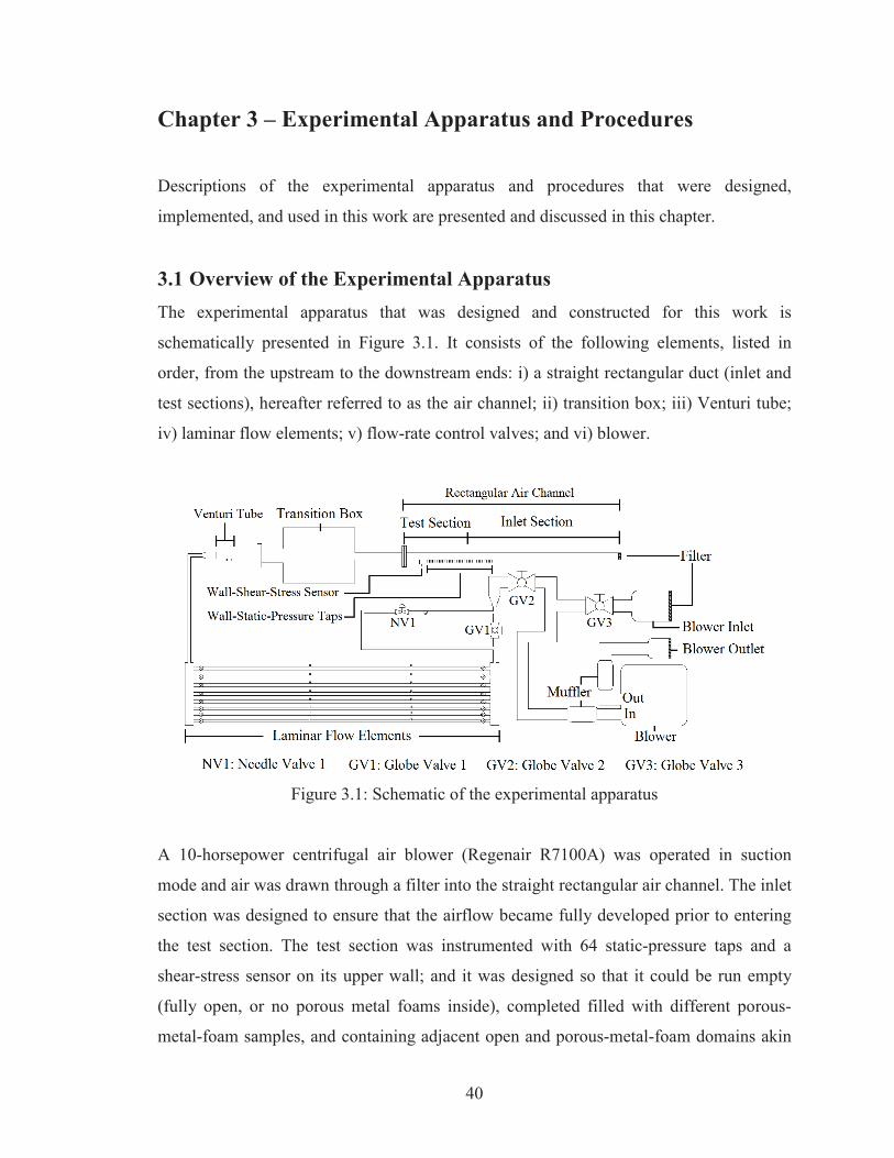
40
Chapter 3 – Experimental Apparatus and Procedures
Descriptions of the experimental apparatus and procedures that were designed,
implemented, and used in this work are presented and discussed in this chapter.
3.1 Overview of the Experimental Apparatus The experimental apparatus that was designed and constructed for this work is
schematically presented in Figure 3.1. It consists of the following elements, listed in
order, from the upstream to the downstream ends: i) a straight rectangular duct (inlet and
test sections), hereafter referred to as the air channel; ii) transition box; iii) Venturi tube;
iv) laminar flow elements; v) flow-rate control valves; and vi) blower.
Figure 3.1: Schematic of the experimental apparatus
A 10-horsepower centrifugal air blower (Regenair R7100A) was operated in suction
mode and air was drawn through a filter into the straight rectangular air channel. The inlet
section was designed to ensure that the airflow became fully developed prior to entering
the test section. The test section was instrumented with 64 static-pressure taps and a
shear-stress sensor on its upper wall; and it was designed so that it could be run empty
(fully open, or no porous metal foams inside), completed filled with different porous-
metal-foam samples, and containing adjacent open and porous-metal-foam domains akin
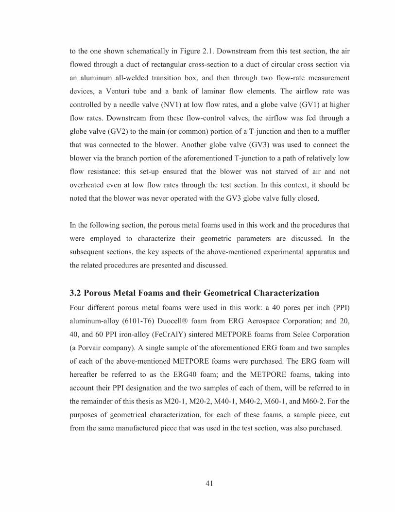
41
to the one shown schematically in Figure 2.1. Downstream from this test section, the air
flowed through a duct of rectangular cross-section to a duct of circular cross section via
an aluminum all-welded transition box, and then through two flow-rate measurement
devices, a Venturi tube and a bank of laminar flow elements. The airflow rate was
controlled by a needle valve (NV1) at low flow rates, and a globe valve (GV1) at higher
flow rates. Downstream from these flow-control valves, the airflow was fed through a
globe valve (GV2) to the main (or common) portion of a T-junction and then to a muffler
that was connected to the blower. Another globe valve (GV3) was used to connect the
blower via the branch portion of the aforementioned T-junction to a path of relatively low
flow resistance: this set-up ensured that the blower was not starved of air and not
overheated even at low flow rates through the test section. In this context, it should be
noted that the blower was never operated with the GV3 globe valve fully closed.
In the following section, the porous metal foams used in this work and the procedures that
were employed to characterize their geometric parameters are discussed. In the
subsequent sections, the key aspects of the above-mentioned experimental apparatus and
the related procedures are presented and discussed.
3.2 Porous Metal Foams and their Geometrical Characterization Four different porous metal foams were used in this work: a 40 pores per inch (PPI)
aluminum-alloy (6101-T6) Duocell® foam from ERG Aerospace Corporation; and 20,
40, and 60 PPI iron-alloy (FeCrAlY) sintered METPORE foams from Selee Corporation
(a Porvair company). A single sample of the aforementioned ERG foam and two samples
of each of the above-mentioned METPORE foams were purchased. The ERG foam will
hereafter be referred to as the ERG40 foam; and the METPORE foams, taking into
account their PPI designation and the two samples of each of them, will be referred to in
the remainder of this thesis as M20-1, M20-2, M40-1, M40-2, M60-1, and M60-2. For the
purposes of geometrical characterization, for each of these foams, a sample piece, cut
from the same manufactured piece that was used in the test section, was also purchased.
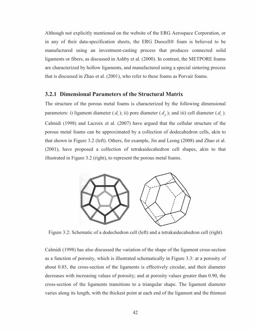
42
Although not explicitly mentioned on the website of the ERG Aerospace Corporation, or
in any of their data-specification sheets, the ERG Duocell® foam is believed to be
manufactured using an investment-casting process that produces connected solid
ligaments or fibers, as discussed in Ashby et al. (2000). In contrast, the METPORE foams
are characterized by hollow ligaments, and manufactured using a special sintering process
that is discussed in Zhao et al. (2001), who refer to these foams as Porvair foams.
3.2.1 Dimensional Parameters of the Structural Matrix The structure of the porous metal foams is characterized by the following dimensional
parameters: i) ligament diameter ( ld ); ii) pore diameter ( pd ); and iii) cell diameter ( cd ).
Calmidi (1998) and Lacroix et al. (2007) have argued that the cellular structure of the
porous metal foams can be approximated by a collection of dodecahedron cells, akin to
that shown in Figure 3.2 (left). Others, for example, Jin and Leong (2008) and Zhao et al.
(2001), have proposed a collection of tetrakaidecahedron cell shapes, akin to that
illustrated in Figure 3.2 (right), to represent the porous metal foams.
Figure 3.2: Schematic of a dodechedron cell (left) and a tetrakaidecahedron cell (right)
Calmidi (1998) has also discussed the variation of the shape of the ligament cross-section
as a function of porosity, which is illustrated schematically in Figure 3.3: at a porosity of
about 0.85, the cross-section of the ligaments is effectively circular, and their diameter
decreases with increasing values of porosity; and at porosity values greater than 0.90, the
cross-section of the ligaments transitions to a triangular shape. The ligament diameter
varies along its length, with the thickest point at each end of the ligament and the thinnest
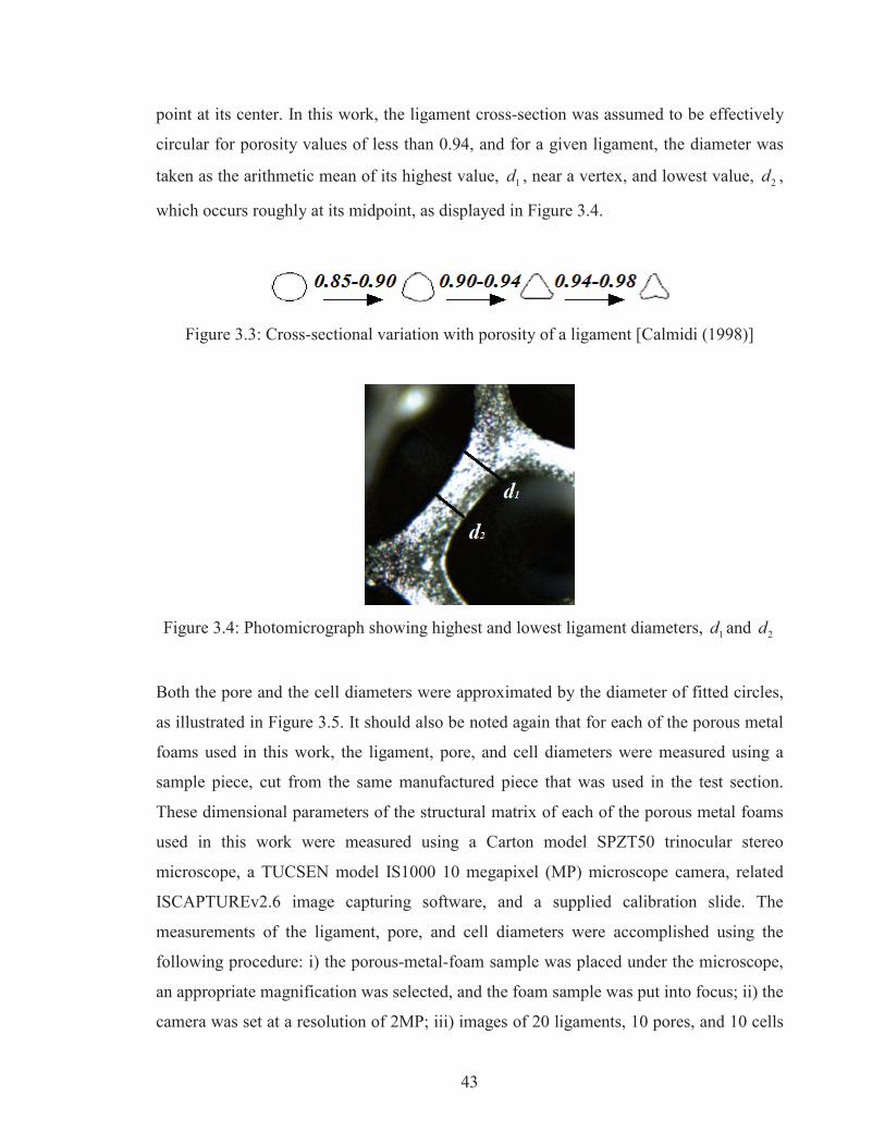
43
point at its center. In this work, the ligament cross-section was assumed to be effectively
circular for porosity values of less than 0.94, and for a given ligament, the diameter was
taken as the arithmetic mean of its highest value, 1d , near a vertex, and lowest value, 2d ,
which occurs roughly at its midpoint, as displayed in Figure 3.4.
Figure 3.3: Cross-sectional variation with porosity of a ligament [Calmidi (1998)]
Figure 3.4: Photomicrograph showing highest and lowest ligament diameters, 1d and 2d
Both the pore and the cell diameters were approximated by the diameter of fitted circles,
as illustrated in Figure 3.5. It should also be noted again that for each of the porous metal
foams used in this work, the ligament, pore, and cell diameters were measured using a
sample piece, cut from the same manufactured piece that was used in the test section.
These dimensional parameters of the structural matrix of each of the porous metal foams
used in this work were measured using a Carton model SPZT50 trinocular stereo
microscope, a TUCSEN model IS1000 10 megapixel (MP) microscope camera, related
ISCAPTUREv2.6 image capturing software, and a supplied calibration slide. The
measurements of the ligament, pore, and cell diameters were accomplished using the
following procedure: i) the porous-metal-foam sample was placed under the microscope,
an appropriate magnification was selected, and the foam sample was put into focus; ii) the
camera was set at a resolution of 2MP; iii) images of 20 ligaments, 10 pores, and 10 cells
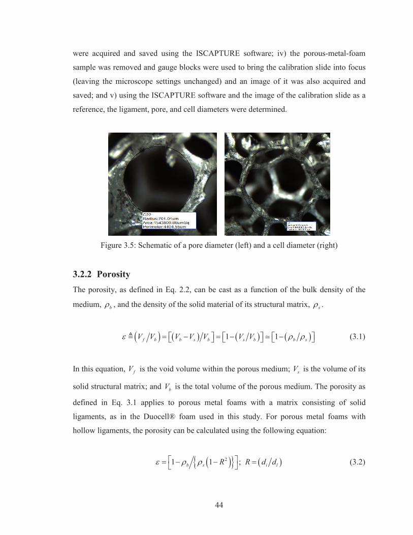
44
were acquired and saved using the ISCAPTURE software; iv) the porous-metal-foam
sample was removed and gauge blocks were used to bring the calibration slide into focus
(leaving the microscope settings unchanged) and an image of it was also acquired and
saved; and v) using the ISCAPTURE software and the image of the calibration slide as a
reference, the ligament, pore, and cell diameters were determined.
Figure 3.5: Schematic of a pore diameter (left) and a cell diameter (right)
3.2.2 Porosity The porosity, as defined in Eq. 2.2, can be cast as a function of the bulk density of the
medium, b , and the density of the solid material of its structural matrix, s .
1 1f b b s b s b b sV V V V V V V (3.1)
In this equation, fV is the void volume within the porous medium; sV is the volume of its
solid structural matrix; and bV is the total volume of the porous medium. The porosity as
defined in Eq. 3.1 applies to porous metal foams with a matrix consisting of solid
ligaments, as in the Duocell® foam used in this study. For porous metal foams with
hollow ligaments, the porosity can be calculated using the following equation:
21 1 ;b s i lR R d d (3.2)
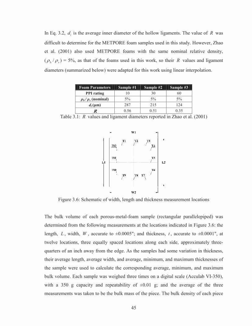
45
In Eq. 3.2, id is the average inner diameter of the hollow ligaments. The value of R was
difficult to determine for the METPORE foam samples used in this study. However, Zhao
et al. (2001) also used METPORE foams with the same nominal relative density,
( /b s ) = 5%, as that of the foams used in this work, so their R values and ligament
diameters (summarized below) were adapted for this work using linear interpolation.
Foam Parameters Sample #1 Sample #2 Sample #3 PPI rating 10 30 60
b s (nominal) 5% 5% 5% dl 287 215 124
0.56 0.51 0.35 Table 3.1: R values and ligament diameters reported in Zhao et al. (2001)
Figure 3.6: Schematic of width, length and thickness measurement locations
The bulk volume of each porous-metal-foam sample (rectangular parallelepiped) was
determined from the following measurements at the locations indicated in Figure 3.6: the
length, L , width, W , accurate to ±0.0005"; and thickness, t , accurate to ±0.0001", at
twelve locations, three equally spaced locations along each side, approximately three-
quarters of an inch away from the edge. As the samples had some variation in thickness,
their average length, average width, and average, minimum, and maximum thicknesses of
the sample were used to calculate the corresponding average, minimum, and maximum
bulk volume. Each sample was weighed three times on a digital scale (Acculab VI-350),
with a 350 g capacity and repeatability of ±0.01 g; and the average of the three
measurements was taken to be the bulk mass of the piece. The bulk density of each piece
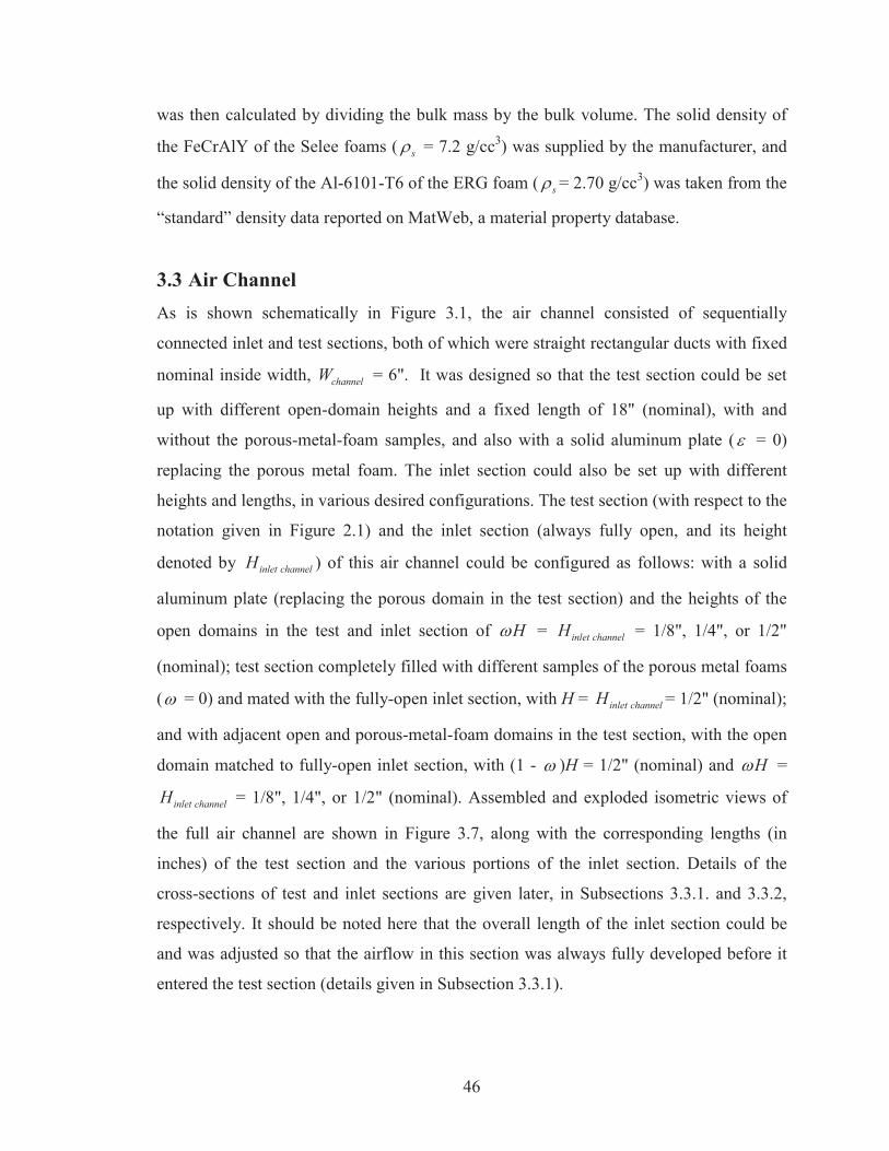
46
was then calculated by dividing the bulk mass by the bulk volume. The solid density of
the FeCrAlY of the Selee foams ( s = 7.2 g/cc3) was supplied by the manufacturer, and
the solid density of the Al-6101-T6 of the ERG foam ( s = 2.70 g/cc3) was taken from the
“standard” density data reported on MatWeb, a material property database.
3.3 Air Channel As is shown schematically in Figure 3.1, the air channel consisted of sequentially
connected inlet and test sections, both of which were straight rectangular ducts with fixed
nominal inside width, channelW = 6". It was designed so that the test section could be set
up with different open-domain heights and a fixed length of 18" (nominal), with and
without the porous-metal-foam samples, and also with a solid aluminum plate ( = 0)
replacing the porous metal foam. The inlet section could also be set up with different
heights and lengths, in various desired configurations. The test section (with respect to the
notation given in Figure 2.1) and the inlet section (always fully open, and its height
denoted by inlet channelH ) of this air channel could be configured as follows: with a solid
aluminum plate (replacing the porous domain in the test section) and the heights of the
open domains in the test and inlet section of H = inlet channelH = 1/8", 1/4", or 1/2"
(nominal); test section completely filled with different samples of the porous metal foams
( = 0) and mated with the fully-open inlet section, with H = inlet channelH = 1/2" (nominal);
and with adjacent open and porous-metal-foam domains in the test section, with the open
domain matched to fully-open inlet section, with (1 - )H = 1/2" (nominal) and H =
inlet channelH = 1/8", 1/4", or 1/2" (nominal). Assembled and exploded isometric views of
the full air channel are shown in Figure 3.7, along with the corresponding lengths (in
inches) of the test section and the various portions of the inlet section. Details of the
cross-sections of test and inlet sections are given later, in Subsections 3.3.1. and 3.3.2,
respectively. It should be noted here that the overall length of the inlet section could be
and was adjusted so that the airflow in this section was always fully developed before it
entered the test section (details given in Subsection 3.3.1).
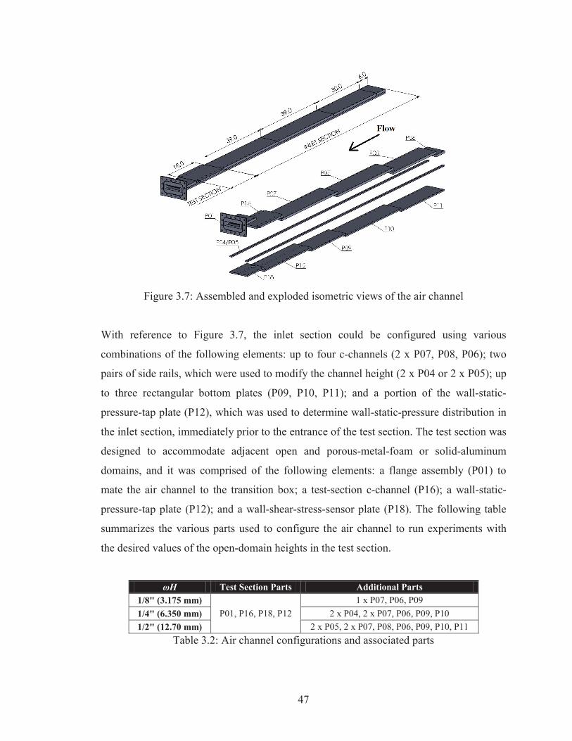
47
Figure 3.7: Assembled and exploded isometric views of the air channel
With reference to Figure 3.7, the inlet section could be configured using various
combinations of the following elements: up to four c-channels (2 x P07, P08, P06); two
pairs of side rails, which were used to modify the channel height (2 x P04 or 2 x P05); up
to three rectangular bottom plates (P09, P10, P11); and a portion of the wall-static-
pressure-tap plate (P12), which was used to determine wall-static-pressure distribution in
the inlet section, immediately prior to the entrance of the test section. The test section was
designed to accommodate adjacent open and porous-metal-foam or solid-aluminum
domains, and it was comprised of the following elements: a flange assembly (P01) to
mate the air channel to the transition box; a test-section c-channel (P16); a wall-static-
pressure-tap plate (P12); and a wall-shear-stress-sensor plate (P18). The following table
summarizes the various parts used to configure the air channel to run experiments with
the desired values of the open-domain heights in the test section.
H Test Section Parts Additional Parts 1/8" (3.175 mm)
P01, P16, P18, P12 1 x P07, P06, P09
1/4" (6.350 mm) 2 x P04, 2 x P07, P06, P09, P10 1/2" (12.70 mm) 2 x P05, 2 x P07, P08, P06, P09, P10, P11
Table 3.2: Air channel configurations and associated parts
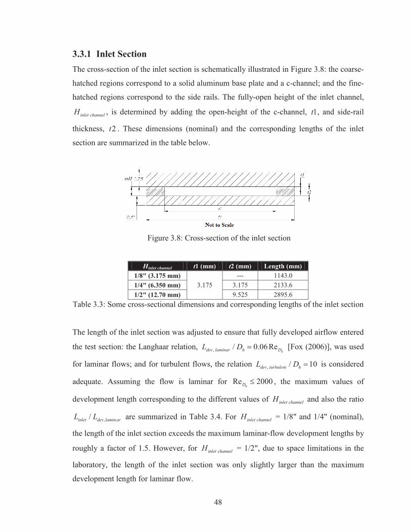
48
3.3.1 Inlet Section The cross-section of the inlet section is schematically illustrated in Figure 3.8: the coarse-
hatched regions correspond to a solid aluminum base plate and a c-channel; and the fine-
hatched regions correspond to the side rails. The fully-open height of the inlet channel,
inlet channelH , is determined by adding the open-height of the c-channel, 1t , and side-rail
thickness, 2t . These dimensions (nominal) and the corresponding lengths of the inlet
section are summarized in the table below.
Figure 3.8: Cross-section of the inlet section
Hinlet channel t1 (mm) t2 (mm) Length (mm) 1/8" (3.175 mm)
3.175 --- 1143.0
1/4" (6.350 mm) 3.175 2133.6 1/2" (12.70 mm) 9.525 2895.6
Table 3.3: Some cross-sectional dimensions and corresponding lengths of the inlet section
The length of the inlet section was adjusted to ensure that fully developed airflow entered
the test section: the Langhaar relation, , / 0.06Rehdev laminar h DL D [Fox (2006)], was used
for laminar flows; and for turbulent flows, the relation , / 10dev turbulent hL D is considered
adequate. Assuming the flow is laminar for Re 2000hD , the maximum values of
development length corresponding to the different values of inlet channelH and also the ratio
,/inlet dev laminarL L are summarized in Table 3.4. For inlet channelH = 1/8" and 1/4" (nominal),
the length of the inlet section exceeds the maximum laminar-flow development lengths by
roughly a factor of 1.5. However, for inlet channelH = 1/2", due to space limitations in the
laboratory, the length of the inlet section was only slightly larger than the maximum
development length for laminar flow.
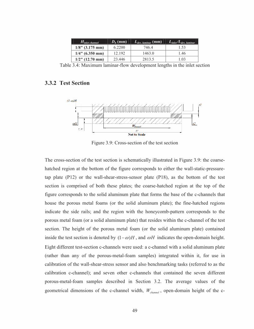
49
Hinlet channel Dh (mm) Ldev, laminar (mm) Linlet /Ldev, laminar
1/8" (3.175 mm) 6.2200 746.4 1.53 1/4" (6.350 mm) 12.192 1463.0 1.46 1/2" (12.70 mm) 23.446 2813.5 1.03
Table 3.4: Maximum laminar-flow development lengths in the inlet section
3.3.2 Test Section
Figure 3.9: Cross-section of the test section
The cross-section of the test section is schematically illustrated in Figure 3.9: the coarse-
hatched region at the bottom of the figure corresponds to either the wall-static-pressure-
tap plate (P12) or the wall-shear-stress-sensor plate (P18), as the bottom of the test
section is comprised of both these plates; the coarse-hatched region at the top of the
figure corresponds to the solid aluminum plate that forms the base of the c-channels that
house the porous metal foams (or the solid aluminum plate); the fine-hatched regions
indicate the side rails; and the region with the honeycomb-pattern corresponds to the
porous metal foam (or a solid aluminum plate) that resides within the c-channel of the test
section. The height of the porous metal foam (or the solid aluminum plate) contained
inside the test section is denoted by (1 )H , and H indicates the open-domain height.
Eight different test-section c-channels were used: a c-channel with a solid aluminum plate
(rather than any of the porous-metal-foam samples) integrated within it, for use in
calibration of the wall-shear-stress sensor and also benchmarking tasks (referred to as the
calibration c-channel); and seven other c-channels that contained the seven different
porous-metal-foam samples described in Section 3.2. The average values of the
geometrical dimensions of the c-channel width, channelW , open-domain height of the c-
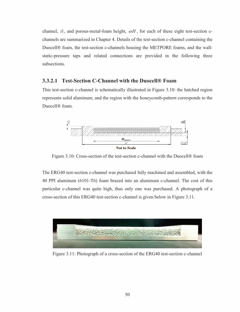
50
channel, 1t , and porous-metal-foam height, H , for each of these eight test-section c-
channels are summarized in Chapter 4. Details of the test-section c-channel containing the
Duocell® foam, the test-section c-channels housing the METPORE foams, and the wall-
static-pressure taps and related connections are provided in the following three
subsections.
3.3.2.1 Test-Section C-Channel with the Duocell® Foam This test-section c-channel is schematically illustrated in Figure 3.10: the hatched region
represents solid aluminum; and the region with the honeycomb-pattern corresponds to the
Duocell® foam.
Figure 3.10: Cross-section of the test-section c-channel with the Duocell® foam
The ERG40 test-section c-channel was purchased fully machined and assembled, with the
40 PPI aluminum (6101-T6) foam brazed into an aluminum c-channel. The cost of this
particular c-channel was quite high, thus only one was purchased. A photograph of a
cross-section of this ERG40 test-section c-channel is given below in Figure 3.11.
Figure 3.11: Photograph of a cross-section of the ERG40 test-section c-channel
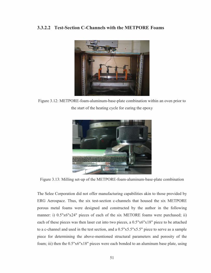
51
3.3.2.2 Test-Section C-Channels with the METPORE Foams
Figure 3.12: METPORE-foam-aluminum-base-plate combination within an oven prior to
the start of the heating cycle for curing the epoxy
Figure 3.13: Milling set-up of the METPORE-foam-aluminum-base-plate combination
The Selee Corporation did not offer manufacturing capabilities akin to those provided by
ERG Aerospace. Thus, the six test-section c-channels that housed the six METPORE
porous metal foams were designed and constructed by the author in the following
manner: i) 0.5"x6"x24" pieces of each of the six METORE foams were purchased; ii)
each of these pieces was then laser cut into two pieces, a 0.5"x6"x18" piece to be attached
to a c-channel and used in the test section, and a 0.5"x5.5"x5.5" piece to serve as a sample
piece for determining the above-mentioned structural parameters and porosity of the
foam; iii) then the 0.5"x6"x18" pieces were each bonded to an aluminum base plate, using
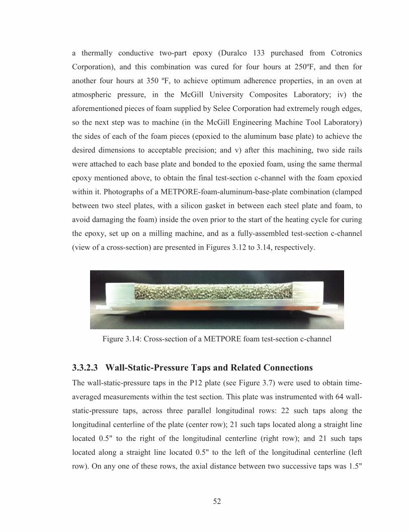
52
a thermally conductive two-part epoxy (Duralco 133 purchased from Cotronics
Corporation), and this combination was cured for four hours at 250ºF, and then for
another four hours at 350 ºF, to achieve optimum adherence properties, in an oven at
atmospheric pressure, in the McGill University Composites Laboratory; iv) the
aforementioned pieces of foam supplied by Selee Corporation had extremely rough edges,
so the next step was to machine (in the McGill Engineering Machine Tool Laboratory)
the sides of each of the foam pieces (epoxied to the aluminum base plate) to achieve the
desired dimensions to acceptable precision; and v) after this machining, two side rails
were attached to each base plate and bonded to the epoxied foam, using the same thermal
epoxy mentioned above, to obtain the final test-section c-channel with the foam epoxied
within it. Photographs of a METPORE-foam-aluminum-base-plate combination (clamped
between two steel plates, with a silicon gasket in between each steel plate and foam, to
avoid damaging the foam) inside the oven prior to the start of the heating cycle for curing
the epoxy, set up on a milling machine, and as a fully-assembled test-section c-channel
(view of a cross-section) are presented in Figures 3.12 to 3.14, respectively.
Figure 3.14: Cross-section of a METPORE foam test-section c-channel
3.3.2.3 Wall-Static-Pressure Taps and Related Connections The wall-static-pressure taps in the P12 plate (see Figure 3.7) were used to obtain time-
averaged measurements within the test section. This plate was instrumented with 64 wall-
static-pressure taps, across three parallel longitudinal rows: 22 such taps along the
longitudinal centerline of the plate (center row); 21 such taps located along a straight line
located 0.5" to the right of the longitudinal centerline (right row); and 21 such taps
located along a straight line located 0.5" to the left of the longitudinal centerline (left
row). On any one of these rows, the axial distance between two successive taps was 1.5"
53
and the first tap on each row was located at an axial distance of 0.75", 1.25", and 1.75"
away from the upstream edge of the wall-static-pressure-tap plate (P12), for the center,
left, and right rows, respectively. These wall-static-pressure taps were numbered from 1
to 64: tap # 1 was the first one on the center row, tap # 2 was the first one on the left row;
tap # 3 was the first tap on the right row; and this sequential numbering pattern was
continued along the length of the plate (P12). The wall-shear-stress-sensor plate (P18)
also included 17 wall-static-pressure taps, similar to those discussed above for plate P12
(they were incorporated into this plate for future works).
At each wall-static-pressure tap location, a #21 (~4.0 mm) diameter hole was first drilled
to a depth of 3/8" (~9.5 mm), and then a 1/32" (~0.8 mm) diameter hole was drilled
through the remainder of the 1/2" (12.7 mm) aluminum plate (P12 or P18), to form the
base of the pressure-tap hole. Threads were then cut into the curved surface of the #21-
diameter hole, using a #10-32 tap, to a depth of 1/4" (~6.4 mm). A Clippard Minimatic
brass pneumatic fitting with a captivated o-ring (Model 11792-5) was then screwed into
the aforementioned tapped hole, and used to connect a 1/16" pressure tubing (Scanivalve
#Vinl-063) to the pressure tap. Although these pneumatic fittings contained a captivated
o-ring, to fully ensure there was no air leakage through the threaded connection of these
fittings to the pressure taps, the base of each fitting was also epoxied in place (after being
screwed into the threaded hole) using a thin bead of Lepage Marine Epoxy.
In this context, it should also be noted that a further 21 blind holes on the P12 plate, and 6
blind holes on P18 plate, were drilled to a depth of 3/8", using a drill of diameter 3/32"
(~2.4 mm): these blind holes are intended for the potting of calibrated thermocouples to
measure the average test-section temperature in future works. In this work, two shielded
and calibrated thermocouples were potted in the aforementioned blind holes in the P12
plate of the air channel, one immediately upstream and the other immediately
downstream of the test section, using a thermally conductive silicone paste (Omega OT-
201). This thermocouple connection was secured to the P12 plate using a combination of
electrical tape (inner layer) and aluminum tape (outer layer).
54
The determination of the test-section wall-static-pressure distributions required multiple
pressure-drop measurements to be taken. For this task, the lines (1/16" pressure tubing)
connected to the test-section-wall-static-pressure taps were connected at their other ends
to a mechanical multiplexer (Scanivalve 48D9), which included a solenoid drive and
controller (Scanivalve model CTLR10(P)/S2-26). The mechanical multiplexor allowed up
to 48 such pressure lines (from the test-section wall-static-pressure taps), and one such
pressure line (connected to a wall-static-pressure tap designated as the reference tap), to
be linked to the differential pressure transducers used in this work. Details of these
differential pressure transducers are presented in Section 3.6. The solenoid-drive
controller was operated using a data acquisition and control unit (HP 3497A), a personal
computer, and a LabVIEW program [Afara (2012)].
3.4 Transition Box An aluminum-alloy (6061-T6) transition box (all-welded construction) was located
downstream of the air channel and upstream of the two flow-measurement sections (the
Venturi tube and the laminar-flow elements), as illustrated in Figure 3.1. This transition
box allowed the air to flow from a rectangular cross-section duct to a duct of circular
cross-section, and had flanges with captivated o-rings to allow airtight connections.
3.5 Flow-Measurement Devices The design, construction, and calibration of two devices for measuring mass flow rates
are described in this section: a Venturi tube for high flow rates; and a bank of laminar-
flow elements (LFEs) for lower flow rates.
3.5.1 Venturi Tube The Venturi tube design and calibration are described in the following two subsections.
3.5.1.1 Design A Venturi tube, with a machined convergent section, was designed in accordance with the
ISO 5167-4:2003 standard. A detailed engineering drawing of this Venturi tube is
provided in Appendix A; and an assembly drawing of the Venturi tube, upstream and
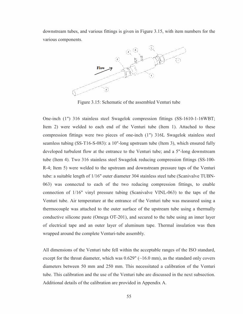
55
downstream tubes, and various fittings is given in Figure 3.15, with item numbers for the
various components.
Figure 3.15: Schematic of the assembled Venturi tube
One-inch (1") 316 stainless steel Swagelok compression fittings (SS-1610-1-16WBT;
Item 2) were welded to each end of the Venturi tube (Item 1). Attached to these
compression fittings were two pieces of one-inch (1") 316L Swagelok stainless steel
seamless tubing (SS-T16-S-083): a 10"-long upstream tube (Item 3), which ensured fully
developed turbulent flow at the entrance to the Venturi tube; and a 5"-long downstream
tube (Item 4). Two 316 stainless steel Swagelok reducing compression fittings (SS-100-
R-4; Item 5) were welded to the upstream and downstream pressure taps of the Venturi
tube: a suitable length of 1/16" outer diameter 304 stainless steel tube (Scanivalve TUBN-
063) was connected to each of the two reducing compression fittings, to enable
connection of 1/16" vinyl pressure tubing (Scanivalve VINL-063) to the taps of the
Venturi tube. Air temperature at the entrance of the Venturi tube was measured using a
thermocouple was attached to the outer surface of the upstream tube using a thermally
conductive silicone paste (Omega OT-201), and secured to the tube using an inner layer
of electrical tape and an outer layer of aluminum tape. Thermal insulation was then
wrapped around the complete Venturi-tube assembly.
All dimensions of the Venturi tube fell within the acceptable ranges of the ISO standard,
except for the throat diameter, which was 0.629" (~16.0 mm), as the standard only covers
diameters between 50 mm and 250 mm. This necessitated a calibration of the Venturi
tube. This calibration and the use of the Venturi tube are discussed in the next subsection.
Additional details of the calibration are provided in Appendix A.
56
3.5.1.2 Calibration The Venturi tube was calibrated at Polycontrols Technologies Inc. (Brossard, Québec).
The calibration data were used to calculate the mass flow rate of air passing through the
Venturi tube, using Eq. 3.3, adapted from the ISO 5167-4:2003 standard (this approach is
necessary to allow accurate determination of the mass flow rates at temperatures and
pressure that are slightly different from those at which the calibration was done).
214
241
VenturiCm d p (3.3)
In Eq. 3.3, Venturim is the mass flow rate through the Venturi tube; C is the discharge
coefficient relating the actual mass flow rate to the theoretical mass flow rate through the
Venturi tube (in the theoretical calculation, C is set equal to 1); is the ratio of the
cylindrical throat diameter to the internal diameter of the upstream cylindrical section;
is the expansibility factor (used to account for the compressibility of air), calculated using
Eq. 3.4; d is the throat diameter; p is the pressure differential between the upstream
and downstream pressure taps; and 1 is the density of air at the upstream pressure tap.
The throat diameter, d , of the Venturi tube was determined to be 0.6290" ±0.0002"; the
internal diameter of the upstream section, D , was measured to be 0.8348" ±0.0001"; so
the diameter ratio, = /d D = 0.7535.
2 4 4 2 ( 1)1 1 1 1 1 ; 0.75 (3.4)
In Eq. 3.4, is the isentropic constant for air, which was taken to be 1.4; and is the
ratio of the throat absolute pressure, 2p , divided by the inlet absolute pressure, 1p .
The discharge coefficient, C , was calculated for each calibration point by dividing the
calibration mass flow rate by the theoretical mass flow rate. In Section 5.5.3 of the ISO
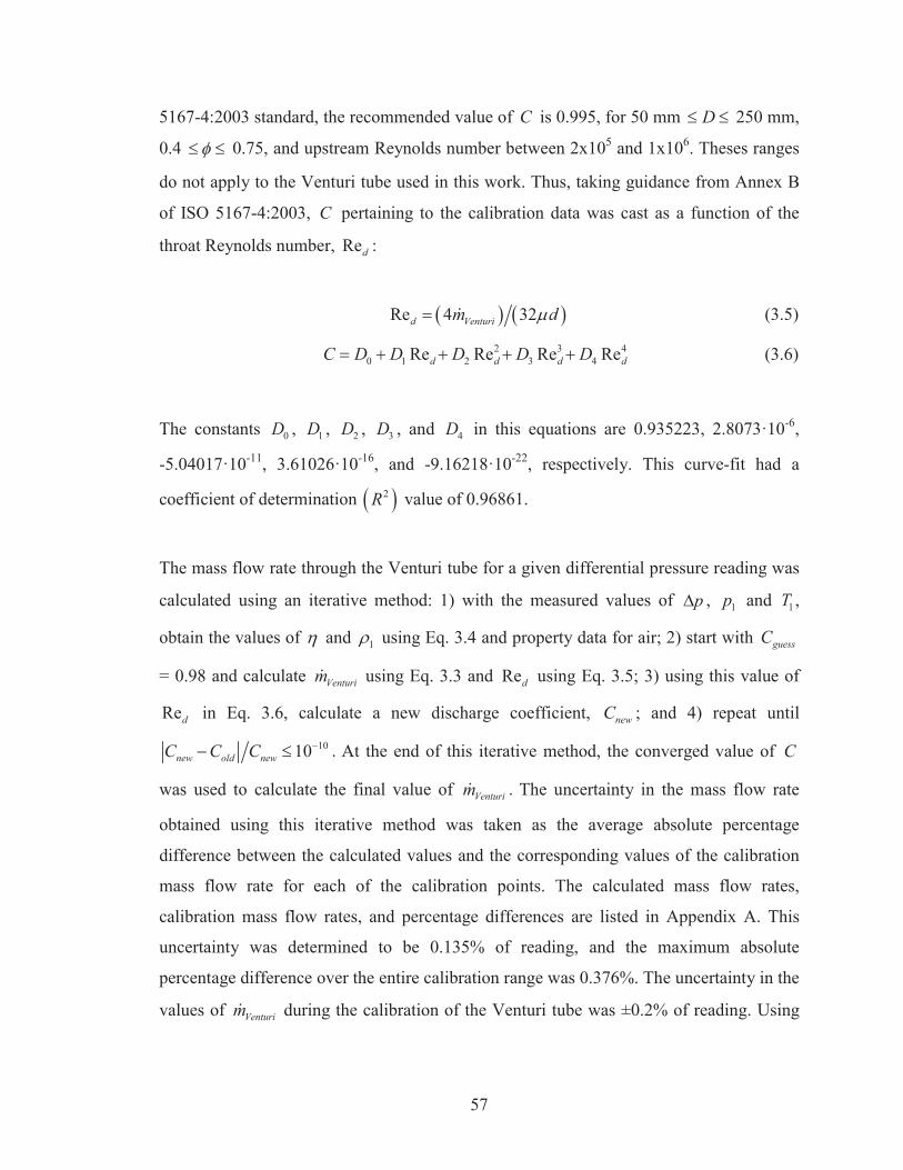
57
5167-4:2003 standard, the recommended value of C is 0.995, for 50 mm D 250 mm,
0.4 0.75, and upstream Reynolds number between 2x10⁵ and 1x10⁶. Theses ranges
do not apply to the Venturi tube used in this work. Thus, taking guidance from Annex B
of ISO 5167-4:2003, C pertaining to the calibration data was cast as a function of the
throat Reynolds number, Red :
Re 4 32d Venturim d (3.5)
2 3 40 1 2 3 4Re Re Re Red d d dC D D D D D (3.6)
The constants 0D , 1D , 2D , 3D , and 4D in this equations are 0.935223, 2.8073·10-6,
-5.04017·10-11, 3.61026·10-16, and -9.16218·10-22, respectively. This curve-fit had a
coefficient of determination 2R value of 0.96861.
The mass flow rate through the Venturi tube for a given differential pressure reading was
calculated using an iterative method: 1) with the measured values of p , 1p and 1T ,
obtain the values of and 1 using Eq. 3.4 and property data for air; 2) start with guessC
= 0.98 and calculate Venturim using Eq. 3.3 and Red using Eq. 3.5; 3) using this value of
Red in Eq. 3.6, calculate a new discharge coefficient, newC ; and 4) repeat until
1010new old newC C C . At the end of this iterative method, the converged value of C
was used to calculate the final value of Venturim . The uncertainty in the mass flow rate
obtained using this iterative method was taken as the average absolute percentage
difference between the calculated values and the corresponding values of the calibration
mass flow rate for each of the calibration points. The calculated mass flow rates,
calibration mass flow rates, and percentage differences are listed in Appendix A. This
uncertainty was determined to be 0.135% of reading, and the maximum absolute
percentage difference over the entire calibration range was 0.376%. The uncertainty in the
values of Venturim during the calibration of the Venturi tube was ±0.2% of reading. Using
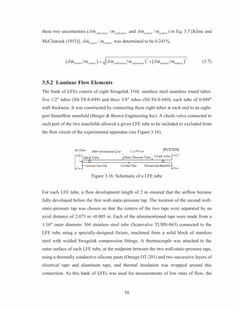
58
these two uncertainties ( /calibration calibrationm m and /method methodm m ) in Eq. 3.7 [Kline and
McClintock (1953)], /Venturi Venturim m was determined to be 0.241%.
2 2Venturi Venturi calibration calibration method methodm m m m m m (3.7)
3.5.2 Laminar Flow Elements The bank of LFEs consist of eight Swagelok 316L stainless steel seamless round tubes:
five 1/2" tubes (SS-T8-S-049) and three 3/8" tubes (SS-T6-S-049), each tube of 0.049"
wall thickness. It was constructed by connecting these eight tubes at each end to an eight-
port Smartflow manifold (Burger & Brown Engineering Inc). A check-valve connected to
each port of the two manifolds allowed a given LFE tube to be included or excluded from
the flow circuit of the experimental apparatus (see Figure 3.16).
Figure 3.16: Schematic of a LFE tube
For each LFE tube, a flow development length of 2 m ensured that the airflow became
fully developed before the first wall-static-pressure tap. The location of the second wall-
static-pressure tap was chosen so that the centers of the two taps were separated by an
axial distance of 2.075 m ±0.005 m. Each of the aforementioned taps were made from a
1/16" outer diameter 304 stainless steel tube (Scanivalve TUBN-063) connected to the
LFE tube using a specially-designed fixture, machined from a solid block of stainless
steel with welded Swagelok compression fittings. A thermocouple was attached to the
outer surface of each LFE tube, at the midpoint between the two wall-static-pressure taps,
using a thermally conductive silicone paste (Omega OT-201) and two successive layers of
electrical tape and aluminum tape, and thermal insulation was wrapped around this
connection. As this bank of LFEs was used for measurements of low rates of flow, the
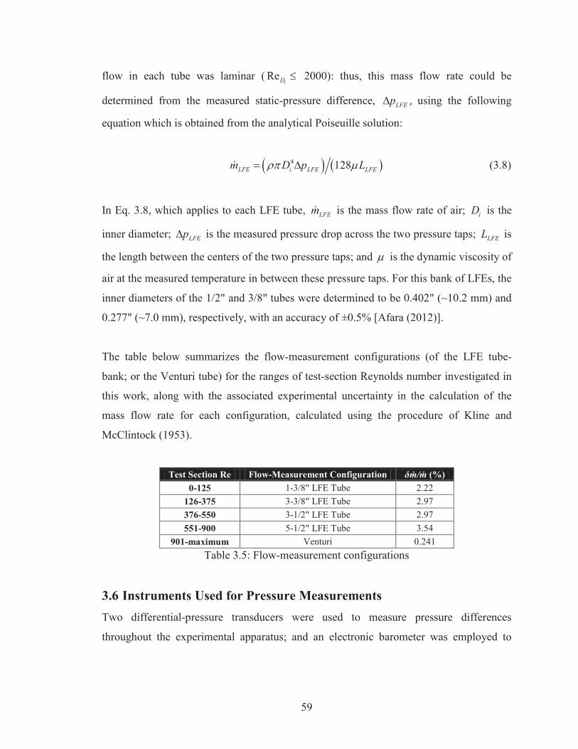
59
flow in each tube was laminar ( ReiD 2000): thus, this mass flow rate could be
determined from the measured static-pressure difference, LFEp , using the following
equation which is obtained from the analytical Poiseuille solution:
4 128LFE i LFE LFEm D p L (3.8)
In Eq. 3.8, which applies to each LFE tube, LFEm is the mass flow rate of air; iD is the
inner diameter; LFEp is the measured pressure drop across the two pressure taps; LFEL is
the length between the centers of the two pressure taps; and is the dynamic viscosity of
air at the measured temperature in between these pressure taps. For this bank of LFEs, the
inner diameters of the 1/2" and 3/8" tubes were determined to be 0.402" (~10.2 mm) and
0.277" (~7.0 mm), respectively, with an accuracy of ±0.5% [Afara (2012)].
The table below summarizes the flow-measurement configurations (of the LFE tube-
bank; or the Venturi tube) for the ranges of test-section Reynolds number investigated in
this work, along with the associated experimental uncertainty in the calculation of the
mass flow rate for each configuration, calculated using the procedure of Kline and
McClintock (1953).
Test Section Re Flow-Measurement Configuration (%) 0-125 1-3/8" LFE Tube 2.22
126-375 3-3/8" LFE Tube 2.97 376-550 3-1/2" LFE Tube 2.97 551-900 5-1/2" LFE Tube 3.54
901-maximum Venturi 0.241 Table 3.5: Flow-measurement configurations
3.6 Instruments Used for Pressure Measurements Two differential-pressure transducers were used to measure pressure differences
throughout the experimental apparatus; and an electronic barometer was employed to
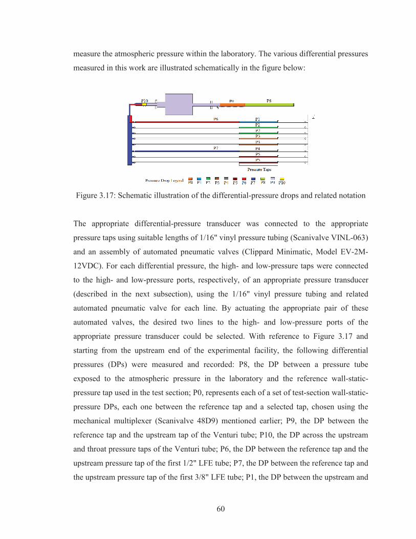
60
measure the atmospheric pressure within the laboratory. The various differential pressures
measured in this work are illustrated schematically in the figure below:
Figure 3.17: Schematic illustration of the differential-pressure drops and related notation
The appropriate differential-pressure transducer was connected to the appropriate
pressure taps using suitable lengths of 1/16" vinyl pressure tubing (Scanivalve VINL-063)
and an assembly of automated pneumatic valves (Clippard Minimatic, Model EV-2M-
12VDC). For each differential pressure, the high- and low-pressure taps were connected
to the high- and low-pressure ports, respectively, of an appropriate pressure transducer
(described in the next subsection), using the 1/16" vinyl pressure tubing and related
automated pneumatic valve for each line. By actuating the appropriate pair of these
automated valves, the desired two lines to the high- and low-pressure ports of the
appropriate pressure transducer could be selected. With reference to Figure 3.17 and
starting from the upstream end of the experimental facility, the following differential
pressures (DPs) were measured and recorded: P8, the DP between a pressure tube
exposed to the atmospheric pressure in the laboratory and the reference wall-static-
pressure tap used in the test section; P0, represents each of a set of test-section wall-static-
pressure DPs, each one between the reference tap and a selected tap, chosen using the
mechanical multiplexer (Scanivalve 48D9) mentioned earlier; P9, the DP between the
reference tap and the upstream tap of the Venturi tube; P10, the DP across the upstream
and throat pressure taps of the Venturi tube; P6, the DP between the reference tap and the
upstream pressure tap of the first 1/2" LFE tube; P7, the DP between the reference tap and
the upstream pressure tap of the first 3/8" LFE tube; P1, the DP between the upstream and
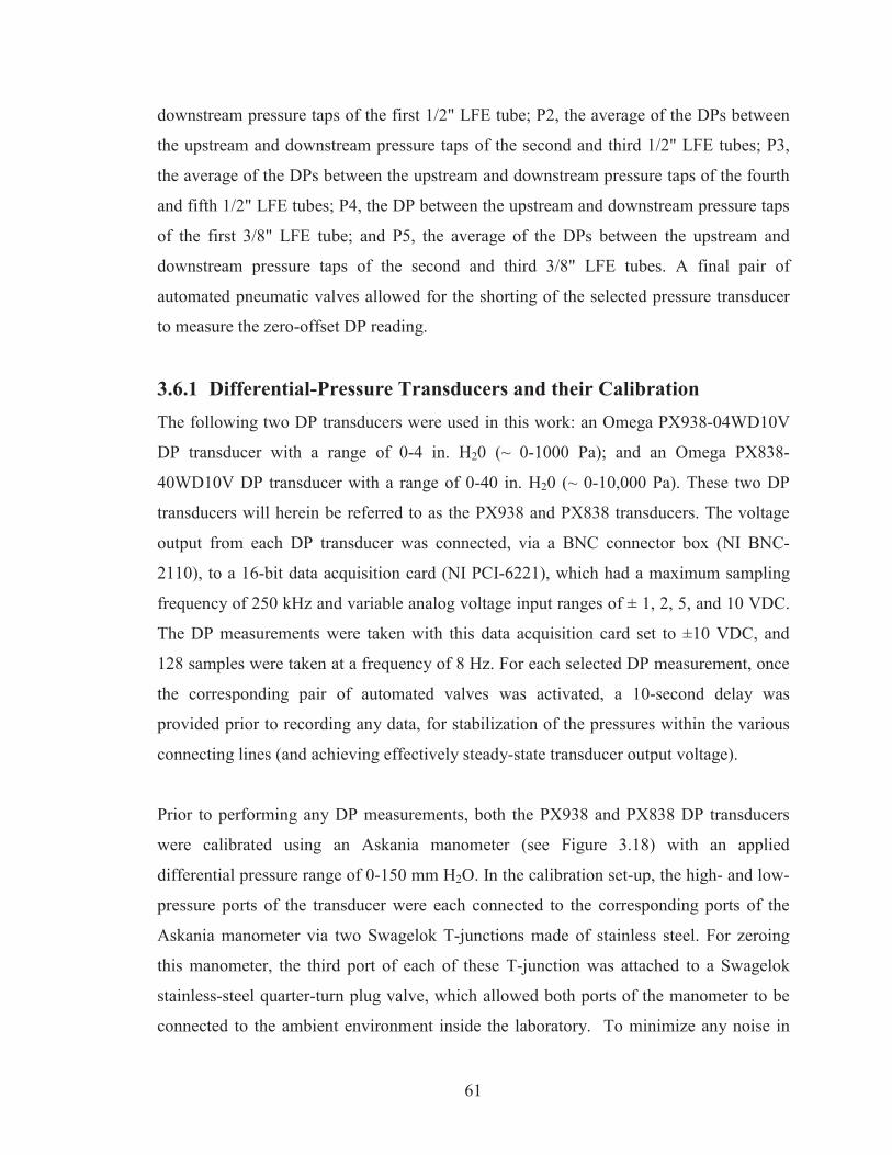
61
downstream pressure taps of the first 1/2" LFE tube; P2, the average of the DPs between
the upstream and downstream pressure taps of the second and third 1/2" LFE tubes; P3,
the average of the DPs between the upstream and downstream pressure taps of the fourth
and fifth 1/2" LFE tubes; P4, the DP between the upstream and downstream pressure taps
of the first 3/8" LFE tube; and P5, the average of the DPs between the upstream and
downstream pressure taps of the second and third 3/8" LFE tubes. A final pair of
automated pneumatic valves allowed for the shorting of the selected pressure transducer
to measure the zero-offset DP reading.
3.6.1 Differential-Pressure Transducers and their Calibration The following two DP transducers were used in this work: an Omega PX938-04WD10V
DP transducer with a range of 0-4 in. H20 (~ 0-1000 Pa); and an Omega PX838-
40WD10V DP transducer with a range of 0-40 in. H20 (~ 0-10,000 Pa). These two DP
transducers will herein be referred to as the PX938 and PX838 transducers. The voltage
output from each DP transducer was connected, via a BNC connector box (NI BNC-
2110), to a 16-bit data acquisition card (NI PCI-6221), which had a maximum sampling
frequency of 250 kHz and variable analog voltage input ranges of ± 1, 2, 5, and 10 VDC.
The DP measurements were taken with this data acquisition card set to ±10 VDC, and
128 samples were taken at a frequency of 8 Hz. For each selected DP measurement, once
the corresponding pair of automated valves was activated, a 10-second delay was
provided prior to recording any data, for stabilization of the pressures within the various
connecting lines (and achieving effectively steady-state transducer output voltage).
Prior to performing any DP measurements, both the PX938 and PX838 DP transducers
were calibrated using an Askania manometer (see Figure 3.18) with an applied
differential pressure range of 0-150 mm H2O. In the calibration set-up, the high- and low-
pressure ports of the transducer were each connected to the corresponding ports of the
Askania manometer via two Swagelok T-junctions made of stainless steel. For zeroing
this manometer, the third port of each of these T-junction was attached to a Swagelok
stainless-steel quarter-turn plug valve, which allowed both ports of the manometer to be
connected to the ambient environment inside the laboratory. To minimize any noise in
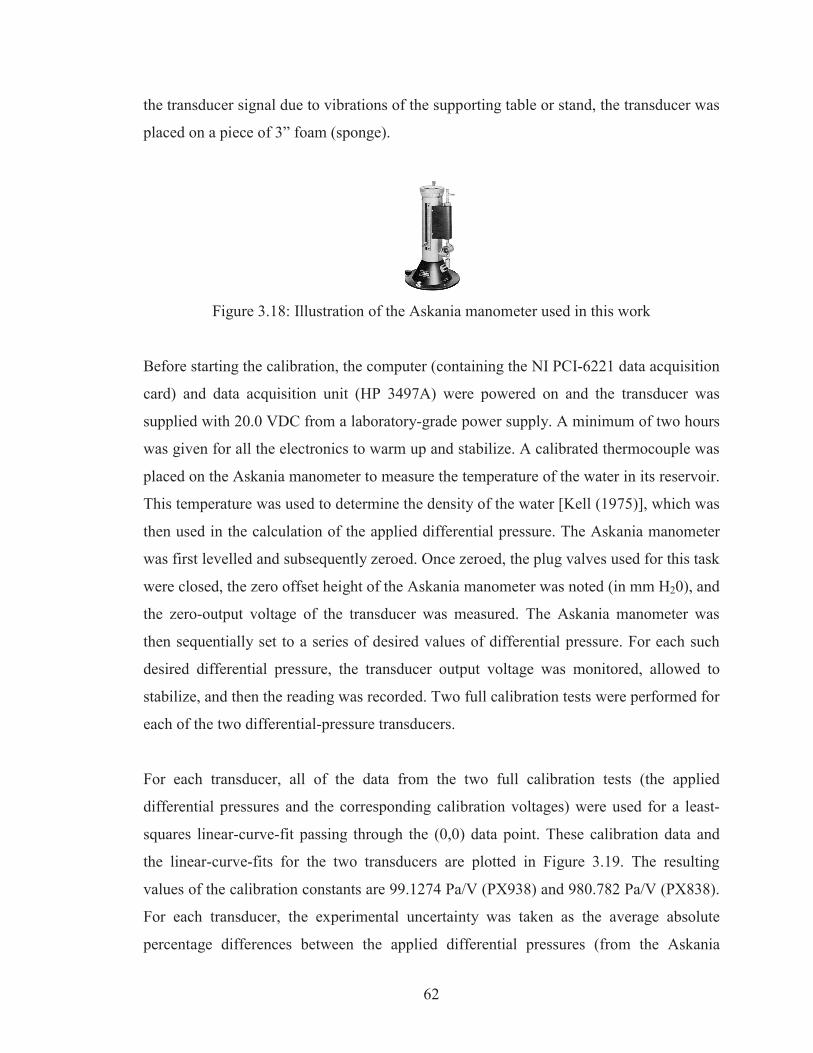
62
the transducer signal due to vibrations of the supporting table or stand, the transducer was
placed on a piece of 3” foam (sponge).
Figure 3.18: Illustration of the Askania manometer used in this work
Before starting the calibration, the computer (containing the NI PCI-6221 data acquisition
card) and data acquisition unit (HP 3497A) were powered on and the transducer was
supplied with 20.0 VDC from a laboratory-grade power supply. A minimum of two hours
was given for all the electronics to warm up and stabilize. A calibrated thermocouple was
placed on the Askania manometer to measure the temperature of the water in its reservoir.
This temperature was used to determine the density of the water [Kell (1975)], which was
then used in the calculation of the applied differential pressure. The Askania manometer
was first levelled and subsequently zeroed. Once zeroed, the plug valves used for this task
were closed, the zero offset height of the Askania manometer was noted (in mm H20), and
the zero-output voltage of the transducer was measured. The Askania manometer was
then sequentially set to a series of desired values of differential pressure. For each such
desired differential pressure, the transducer output voltage was monitored, allowed to
stabilize, and then the reading was recorded. Two full calibration tests were performed for
each of the two differential-pressure transducers.
For each transducer, all of the data from the two full calibration tests (the applied
differential pressures and the corresponding calibration voltages) were used for a least-
squares linear-curve-fit passing through the (0,0) data point. These calibration data and
the linear-curve-fits for the two transducers are plotted in Figure 3.19. The resulting
values of the calibration constants are 99.1274 Pa/V (PX938) and 980.782 Pa/V (PX838).
For each transducer, the experimental uncertainty was taken as the average absolute
percentage differences between the applied differential pressures (from the Askania
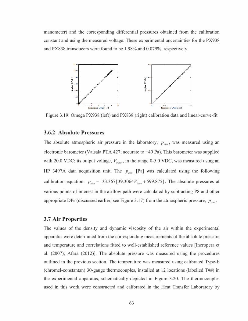
63
manometer) and the corresponding differential pressures obtained from the calibration
constant and using the measured voltage. These experimental uncertainties for the PX938
and PX838 transducers were found to be 1.98% and 0.079%, respectively.
Figure 3.19: Omega PX938 (left) and PX838 (right) calibration data and linear-curve-fit
3.6.2 Absolute Pressures
The absolute atmospheric air pressure in the laboratory, atmp , was measured using an
electronic barometer (Vaisala PTA 427; accurate to ±40 Pa). This barometer was supplied
with 20.0 VDC; its output voltage, baroV , in the range 0-5.0 VDC, was measured using an
HP 3497A data acquisition unit. The atmp [Pa] was calculated using the following
calibration equation: 133.367 39.3064 599.875atm barop V . The absolute pressures at
various points of interest in the airflow path were calculated by subtracting P8 and other
appropriate DPs (discussed earlier; see Figure 3.17) from the atmospheric pressure, atmp .
3.7 Air Properties The values of the density and dynamic viscosity of the air within the experimental
apparatus were determined from the corresponding measurements of the absolute pressure
and temperature and correlations fitted to well-established reference values [Incropera et
al. (2007); Afara (2012)]. The absolute pressure was measured using the procedures
outlined in the previous section. The temperature was measured using calibrated Type-E
(chromel-constantan) 30-gauge thermocouples, installed at 12 locations (labelled T##) in
the experimental apparatus, schematically depicted in Figure 3.20. The thermocouples
used in this work were constructed and calibrated in the Heat Transfer Laboratory by
64
Afara (2012), over the range 5-62 ºC with an accuracy of ±0.02 ºC, and connected to an
Omega thermocouple connector box, which was then connected to the HP 3497A data
acquisition unit. Each temperature measurement was taken as the average of 25 readings
of the corresponding thermocouple, taken at a frequency of 4 Hz, using a specially
designed LabVIEW program written by Afara (2012). With reference to the notation in
Figure 3.20, starting at the upstream end of the experimental apparatus, the above-
mentioned thermocouples (T40-T51) were used to measure temperature at the following
locations: T49, inlet to the air tunnel; T40, test-section inlet; T50, test-section outlet; T51,
the Venturi-tube inlet; and T41-T48, the eight LFE tubes.
Figure 3.20: Schematic illustration of the locations of the temperature measurements
3.8 Set-up for Permeability and Dimensionless Form-Drag Coefficient In this set-up, the air channel was configured for airflow only through the metal foam in
each of the test-section c-channels discussed earlier. In this configuration, with reference
to Figure 3.7, the wall-static-pressure-tap plate (P12) was positioned to allow
measurement of the wall-static-pressure distribution over the full length (18") of the metal
foam in the test-section c-channels. The inlet section of the air channel was configured to
the nominal 1/2" height, and the test section was configured to the nominal 1/8" open-
domain height. To ensure the air did not flow within the open-domain of the test section
in this configuration, a variety of gaskets were used. The gaskets were purchased from
Stockwell Elastomerics Inc. They were made of BISCO® BF-2000 ultra-soft silicone
foam and had thicknesses that were approximately 40-50% larger than the measured
open-domain gap heights of the test-section metal-foam c-channels, to ensure proper
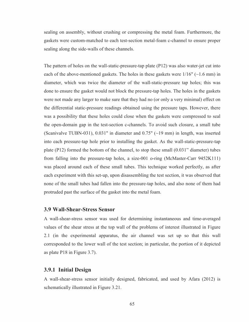
65
sealing on assembly, without crushing or compressing the metal foam. Furthermore, the
gaskets were custom-matched to each test-section metal-foam c-channel to ensure proper
sealing along the side-walls of these channels.
The pattern of holes on the wall-static-pressure-tap plate (P12) was also water-jet cut into
each of the above-mentioned gaskets. The holes in these gaskets were 1/16" (~1.6 mm) in
diameter, which was twice the diameter of the wall-static-pressure tap holes; this was
done to ensure the gasket would not block the pressure-tap holes. The holes in the gaskets
were not made any larger to make sure that they had no (or only a very minimal) effect on
the differential static-pressure readings obtained using the pressure taps. However, there
was a possibility that these holes could close when the gaskets were compressed to seal
the open-domain gap in the test-section c-channels. To avoid such closure, a small tube
(Scanivalve TUBN-031), 0.031" in diameter and 0.75" (~19 mm) in length, was inserted
into each pressure-tap hole prior to installing the gasket. As the wall-static-pressure-tap
plate (P12) formed the bottom of the channel, to stop these small (0.031” diameter) tubes
from falling into the pressure-tap holes, a size-001 o-ring (McMaster-Carr 9452K111)
was placed around each of these small tubes. This technique worked perfectly, as after
each experiment with this set-up, upon disassembling the test section, it was observed that
none of the small tubes had fallen into the pressure-tap holes, and also none of them had
protruded past the surface of the gasket into the metal foam.
3.9 Wall-Shear-Stress Sensor A wall-shear-stress sensor was used for determining instantaneous and time-averaged
values of the shear stress at the top wall of the problems of interest illustrated in Figure
2.1 (in the experimental apparatus, the air channel was set up so that this wall
corresponded to the lower wall of the test section; in particular, the portion of it depicted
as plate P18 in Figure 3.7).
3.9.1 Initial Design A wall-shear-stress sensor initially designed, fabricated, and used by Afara (2012) is
schematically illustrated in Figure 3.21.
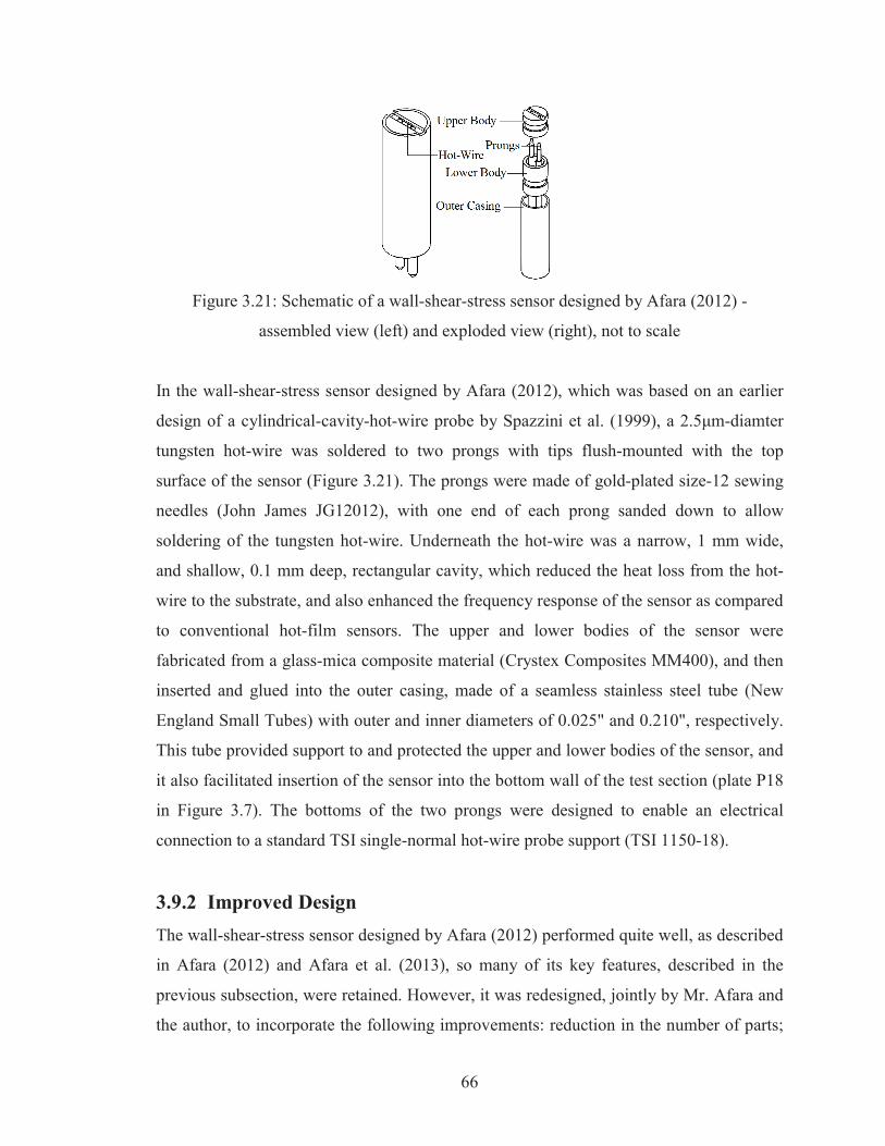
66
Figure 3.21: Schematic of a wall-shear-stress sensor designed by Afara (2012) -
assembled view (left) and exploded view (right), not to scale
In the wall-shear-stress sensor designed by Afara (2012), which was based on an earlier
design of a cylindrical-cavity-hot- -diamter
tungsten hot-wire was soldered to two prongs with tips flush-mounted with the top
surface of the sensor (Figure 3.21). The prongs were made of gold-plated size-12 sewing
needles (John James JG12012), with one end of each prong sanded down to allow
soldering of the tungsten hot-wire. Underneath the hot-wire was a narrow, 1 mm wide,
and shallow, 0.1 mm deep, rectangular cavity, which reduced the heat loss from the hot-
wire to the substrate, and also enhanced the frequency response of the sensor as compared
to conventional hot-film sensors. The upper and lower bodies of the sensor were
fabricated from a glass-mica composite material (Crystex Composites MM400), and then
inserted and glued into the outer casing, made of a seamless stainless steel tube (New
England Small Tubes) with outer and inner diameters of 0.025" and 0.210", respectively.
This tube provided support to and protected the upper and lower bodies of the sensor, and
it also facilitated insertion of the sensor into the bottom wall of the test section (plate P18
in Figure 3.7). The bottoms of the two prongs were designed to enable an electrical
connection to a standard TSI single-normal hot-wire probe support (TSI 1150-18).
3.9.2 Improved Design The wall-shear-stress sensor designed by Afara (2012) performed quite well, as described
in Afara (2012) and Afara et al. (2013), so many of its key features, described in the
previous subsection, were retained. However, it was redesigned, jointly by Mr. Afara and
the author, to incorporate the following improvements: reduction in the number of parts;
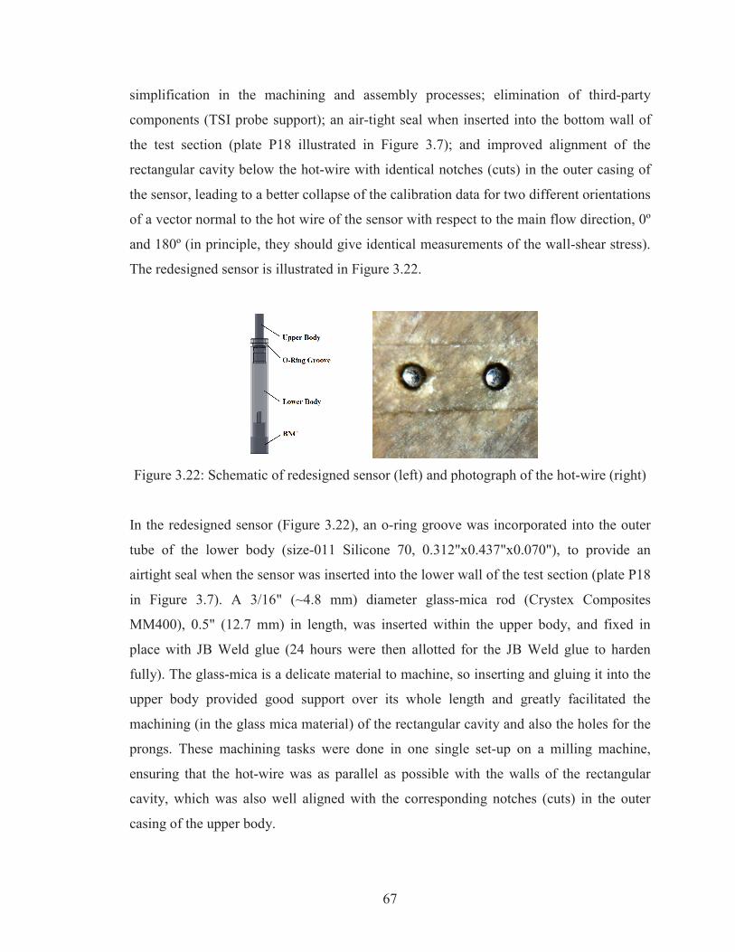
67
simplification in the machining and assembly processes; elimination of third-party
components (TSI probe support); an air-tight seal when inserted into the bottom wall of
the test section (plate P18 illustrated in Figure 3.7); and improved alignment of the
rectangular cavity below the hot-wire with identical notches (cuts) in the outer casing of
the sensor, leading to a better collapse of the calibration data for two different orientations
of a vector normal to the hot wire of the sensor with respect to the main flow direction, 0º
and 180º (in principle, they should give identical measurements of the wall-shear stress).
The redesigned sensor is illustrated in Figure 3.22.
Figure 3.22: Schematic of redesigned sensor (left) and photograph of the hot-wire (right)
In the redesigned sensor (Figure 3.22), an o-ring groove was incorporated into the outer
tube of the lower body (size-011 Silicone 70, 0.312"x0.437"x0.070"), to provide an
airtight seal when the sensor was inserted into the lower wall of the test section (plate P18
in Figure 3.7). A 3/16" (~4.8 mm) diameter glass-mica rod (Crystex Composites
MM400), 0.5" (12.7 mm) in length, was inserted within the upper body, and fixed in
place with JB Weld glue (24 hours were then allotted for the JB Weld glue to harden
fully). The glass-mica is a delicate material to machine, so inserting and gluing it into the
upper body provided good support over its whole length and greatly facilitated the
machining (in the glass mica material) of the rectangular cavity and also the holes for the
prongs. These machining tasks were done in one single set-up on a milling machine,
ensuring that the hot-wire was as parallel as possible with the walls of the rectangular
cavity, which was also well aligned with the corresponding notches (cuts) in the outer
casing of the upper body.
68
In the redesigned sensor, the ends of the prongs away from the soldered hot-wire were not
connected to a TSI probe support. Rather, a piece of insulated 22-gauge solid aluminum
wire was soldered to this end of each of the two prongs; and then the other ends of the
two solid aluminum wires were soldered to a 50-
connector (Digi-Key Corporation ACX1048-ND). Following these steps, a shorting
fixture and a procedure similar to that outlined in Afara (2012) was used to determine the
combined electrical resistance of the two prongs of the new sensor, prR . This resistance is
needed for calculating the cold-wire electrical resistance of the sensor (which, in turn, is
necessary for determining its operating resistance, as is discussed in the next subsection).
Once the combined electrical resistance of the prongs was determined, the following
sensor-assembly steps were followed sequentially: i) the female BNC connector was de-
soldered from the ends of the two 22 gauge wires (which remained soldered to the prongs
at their other ends); ii) the prongs were inserted into the holes drilled for them in the
upper body, and they were then pushed through these holes so that their ends protruded
from the top surface of the upper body; iii) these ends of the prongs were then pressed
against a precision-ground flat gauge block to make them flush with the top surface of the
upper body; iv) a low-electrical- and low-thermal-conductivity epoxy (Cotronics EE4525)
was then injected into the bottom of the upper body, until all openings and cavities were
entirely filled with this epoxy, and the assembly was left undisturbed for 24 hours to
allow the epoxy to cure and harden fully; v) the female BNC connector was again
soldered to the ends of the two 22 gauge wires; vi) JB Weld glue was applied to the
bottom of the assembled upper body and around the threads of the female BNC
connector; vii) the upper-body assembly was then inserted through the lower body and
mounted within a jig, mimicking the sensor-mounting block used in the test section
(discussed in the next subsection), to ensure that the upper and lower bodies are
concentrically aligned; and viii) the complete assembly was left undisturbed for another
24 hours to allow full hardening of the JB Weld glue. At this stage, the body of the
sensor, its prongs, and connector are completely assembled. A hot-wire was then soldered
to the tips of the two prongs (see Figure 3.22), using a special procedure that is outlined
fully in Afara (2012), so it is not be repeated here.
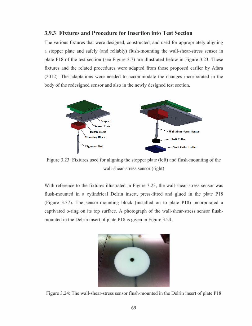
69
3.9.3 Fixtures and Procedure for Insertion into Test Section The various fixtures that were designed, constructed, and used for appropriately aligning
a stopper plate and safely (and reliably) flush-mounting the wall-shear-stress sensor in
plate P18 of the test section (see Figure 3.7) are illustrated below in Figure 3.23. These
fixtures and the related procedures were adapted from those proposed earlier by Afara
(2012). The adaptations were needed to accommodate the changes incorporated in the
body of the redesigned sensor and also in the newly designed test section.
Figure 3.23: Fixtures used for aligning the stopper plate (left) and flush-mounting of the
wall-shear-stress sensor (right)
With reference to the fixtures illustrated in Figure 3.23, the wall-shear-stress sensor was
flush-mounted in a cylindrical Delrin insert, press-fitted and glued in the plate P18
(Figure 3.37). The sensor-mounting block (installed on to plate P18) incorporated a
captivated o-ring on its top surface. A photograph of the wall-shear-stress sensor flush-
mounted in the Delrin insert of plate P18 is given in Figure 3.24.
Figure 3.24: The wall-shear-stress sensor flush-mounted in the Delrin insert of plate P18
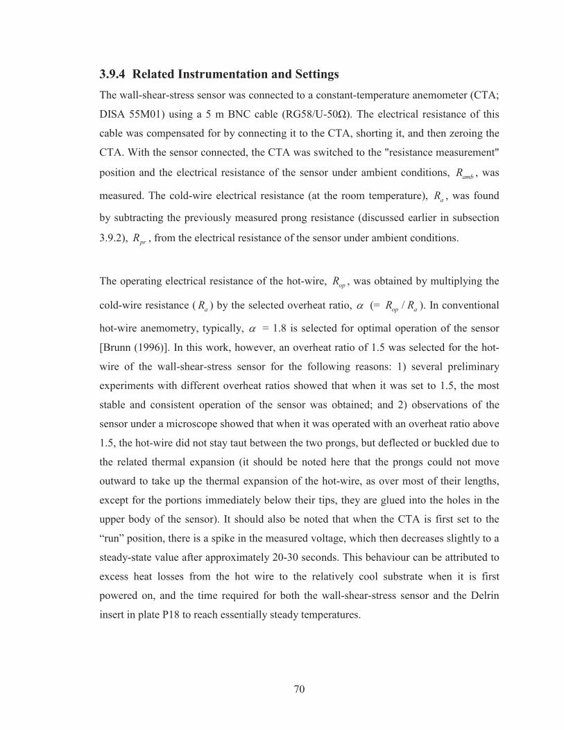
70
3.9.4 Related Instrumentation and Settings The wall-shear-stress sensor was connected to a constant-temperature anemometer (CTA;
DISA 55M01) using a 5 m BNC cable (RG58/U-
cable was compensated for by connecting it to the CTA, shorting it, and then zeroing the
CTA. With the sensor connected, the CTA was switched to the "resistance measurement"
position and the electrical resistance of the sensor under ambient conditions, ambR , was
measured. The cold-wire electrical resistance (at the room temperature), aR , was found
by subtracting the previously measured prong resistance (discussed earlier in subsection
3.9.2), prR , from the electrical resistance of the sensor under ambient conditions.
The operating electrical resistance of the hot-wire, opR , was obtained by multiplying the
cold-wire resistance ( aR ) by the selected overheat ratio, (= /op aR R ). In conventional
hot-wire anemometry, typically, = 1.8 is selected for optimal operation of the sensor
[Brunn (1996)]. In this work, however, an overheat ratio of 1.5 was selected for the hot-
wire of the wall-shear-stress sensor for the following reasons: 1) several preliminary
experiments with different overheat ratios showed that when it was set to 1.5, the most
stable and consistent operation of the sensor was obtained; and 2) observations of the
sensor under a microscope showed that when it was operated with an overheat ratio above
1.5, the hot-wire did not stay taut between the two prongs, but deflected or buckled due to
the related thermal expansion (it should be noted here that the prongs could not move
outward to take up the thermal expansion of the hot-wire, as over most of their lengths,
except for the portions immediately below their tips, they are glued into the holes in the
upper body of the sensor). It should also be noted that when the CTA is first set to the
“run” position, there is a spike in the measured voltage, which then decreases slightly to a
steady-state value after approximately 20-30 seconds. This behaviour can be attributed to
excess heat losses from the hot wire to the relatively cool substrate when it is first
powered on, and the time required for both the wall-shear-stress sensor and the Delrin
insert in plate P18 to reach essentially steady temperatures.
71
In this work, the sensor was aligned (that is, its hot-wire was oriented) to yield the
maximum CTA voltage output at a test-section Reynolds number of approximately 2000,
and then this alignment was maintained during all subsequent calibrations and
measurements. As the calibrations and all subsequent measurements were done with the
sensor inserted in the same plate (P18) and maintained in the same position, heat losses
from the hot wire to the Delrin piece (inserted in plate P18) were intrinsically taken into
account, and there was also no need for concern about any errors resulting from angular
or flush-mounting off-sets. Nevertheless, special care was taken to ensure that the sensor
was indeed flush-mounted and remained in the aforementioned alignment during the
calibrations and also during all subsequent measurements.
3.9.5 Calibration This task was done using the calibration c-channel discussed earlier in Subsection 3.3.2,
with the test section configured to achieve three different open-domain heights. For
laminar flows ( Re 2000), the analytical solution (Subsection 2.6.1, Eq. 2.30) was used
to obtain the following relationship between the time-averaged wall-shear stress, w , and
the average velocity, avu , in the test section:
2
0
50
11 82 cosh
tanh1 8 ; ; (2 1)12 2
avw
n n n
n channeln
n n
uUH
WU nH
(3.9)
For fully developed turbulent flows in straight ducts of rectangular cross-section, an
empirical correlation proposed by Zanoun et al (2003) was used for calibrating the wall-
shear-stress sensor. Their correlation applies to an aspect ratio (width/height) of 12:1,
which corresponds to the lowest value of aspect ratio considered in this work, and values
of Reynolds numbers (based on wall-friction velocity) greater than those investigated in
this work. Thus, before using this correlation for calibrating the wall-shear-stress sensor,
it was benchmarked for the turbulent flows investigated in this work (4000 Re
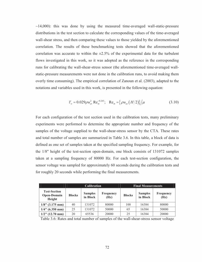
72
~14,000): this was done by using the measured time-averaged wall-static-pressure
distributions in the test section to calculate the corresponding values of the time-averaged
wall-shear stress, and then comparing these values to those yielded by the aforementioned
correlation. The results of these benchmarking tests showed that the aforementioned
correlation was accurate to within the ±2.5% of the experimental data for the turbulent
flows investigated in this work, so it was adopted as the reference in the corresponding
runs for calibrating the wall-shear-stress sensor (the aforementioned time-averaged wall-
static-pressure measurements were not done in the calibration runs, to avoid making them
overly time consuming). The empirical correlation of Zanoun et al. (2003), adapted to the
notations and variables used in this work, is presented in the following equation:
2 0.2430.029 Re ; Re 2w av m m avu u H (3.10)
For each configuration of the test section used in the calibration tests, many preliminary
experiments were performed to determine the appropriate number and frequency of the
samples of the voltage supplied to the wall-shear-stress sensor by the CTA. These rates
and total number of samples are summarized in Table 3.6. In this table, a block of data is
defined as one set of samples taken at the specified sampling frequency. For example, for
the 1/8" height of the test-section open-domain, one block consists of 131072 samples
taken at a sampling frequency of 80000 Hz. For each test-section configuration, the
sensor voltage was sampled for approximately 60 seconds during the calibration tests and
for roughly 20 seconds while performing the final measurements.
Calibration Final Measurements
Test-Section Open-Domain
Height Blocks Samples
in Block Frequency
(Hz) Blocks Samples in Block
Frequency (Hz)
1/8" (3.175 mm) 40 131072 80000 100 16384 80000 1/4" (6.350 mm) 25 131072 50000 65 16384 50000 1/2" (12.70 mm) 20 65536 20000 25 16384 20000 Table 3.6: Rates and total number of samples of the wall-shear-stress sensor voltage
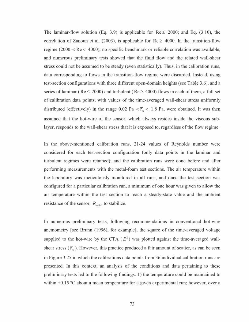
73
The laminar-flow solution (Eq. 3.9) is applicable for Re 2000; and Eq. (3.10), the
correlation of Zanoun et al. (2003), is applicable for Re 4000. In the transition-flow
regime (2000 Re 4000), no specific benchmark or reliable correlation was available,
and numerous preliminary tests showed that the fluid flow and the related wall-shear
stress could not be assumed to be steady (even statistically). Thus, in the calibration runs,
data corresponding to flows in the transition-flow regime were discarded. Instead, using
test-section configurations with three different open-domain heights (see Table 3.6), and a
series of laminar ( Re 2000) and turbulent ( Re 4000) flows in each of them, a full set
of calibration data points, with values of the time-averaged wall-shear stress uniformly
distributed (effectively) in the range 0.02 Pa w 1.8 Pa, were obtained. It was then
assumed that the hot-wire of the sensor, which always resides inside the viscous sub-
layer, responds to the wall-shear stress that it is exposed to, regardless of the flow regime.
In the above-mentioned calibration runs, 21-24 values of Reynolds number were
considered for each test-section configuration (only data points in the laminar and
turbulent regimes were retained); and the calibration runs were done before and after
performing measurements with the metal-foam test sections. The air temperature within
the laboratory was meticulously monitored in all runs, and once the test section was
configured for a particular calibration run, a minimum of one hour was given to allow the
air temperature within the test section to reach a steady-state value and the ambient
resistance of the sensor, ambR , to stabilize.
In numerous preliminary tests, following recommendations in conventional hot-wire
anemometry [see Brunn (1996), for example], the square of the time-averaged voltage
supplied to the hot-wire by the CTA ( 2E ) was plotted against the time-averaged wall-
shear stress ( w ). However, this practice produced a fair amount of scatter, as can be seen
in Figure 3.25 in which the calibrations data points from 36 individual calibration runs are
presented. In this context, an analysis of the conditions and data pertaining to these
preliminary tests led to the following findings: 1) the temperature could be maintained to
within ±0.15 ºC about a mean temperature for a given experimental run; however, over a
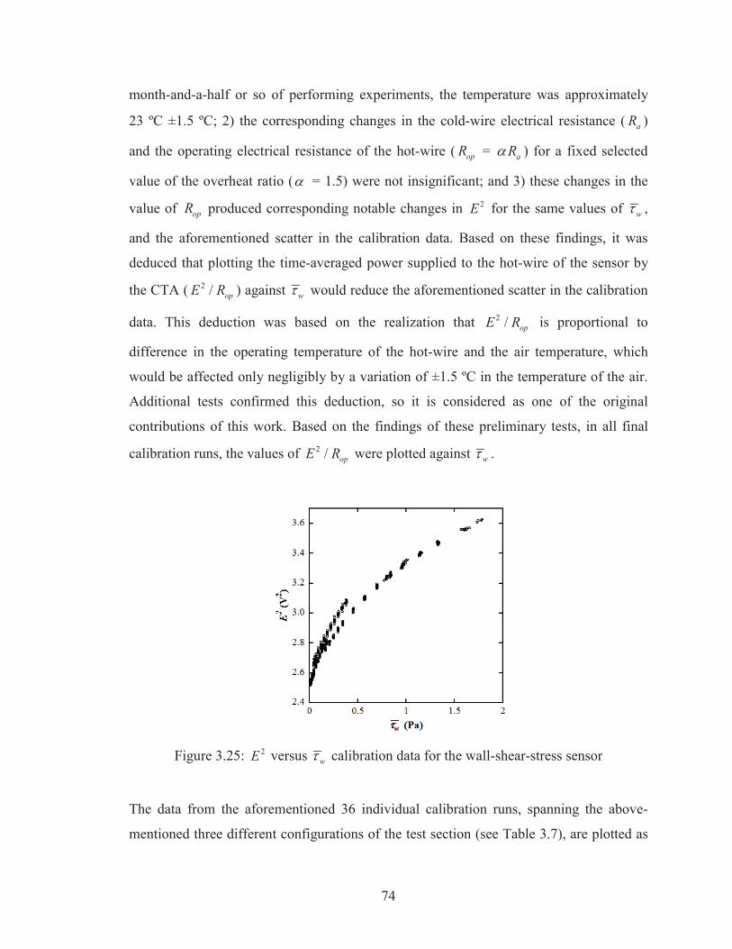
74
month-and-a-half or so of performing experiments, the temperature was approximately
23 ºC ±1.5 ºC; 2) the corresponding changes in the cold-wire electrical resistance ( aR )
and the operating electrical resistance of the hot-wire ( opR = aR ) for a fixed selected
value of the overheat ratio ( = 1.5) were not insignificant; and 3) these changes in the
value of opR produced corresponding notable changes in 2E for the same values of w ,
and the aforementioned scatter in the calibration data. Based on these findings, it was
deduced that plotting the time-averaged power supplied to the hot-wire of the sensor by
the CTA ( 2 / opE R ) against w would reduce the aforementioned scatter in the calibration
data. This deduction was based on the realization that 2 / opE R is proportional to
difference in the operating temperature of the hot-wire and the air temperature, which
would be affected only negligibly by a variation of ±1.5 ºC in the temperature of the air.
Additional tests confirmed this deduction, so it is considered as one of the original
contributions of this work. Based on the findings of these preliminary tests, in all final
calibration runs, the values of 2 / opE R were plotted against w .
Figure 3.25: 2E versus w calibration data for the wall-shear-stress sensor
The data from the aforementioned 36 individual calibration runs, spanning the above-
mentioned three different configurations of the test section (see Table 3.7), are plotted as
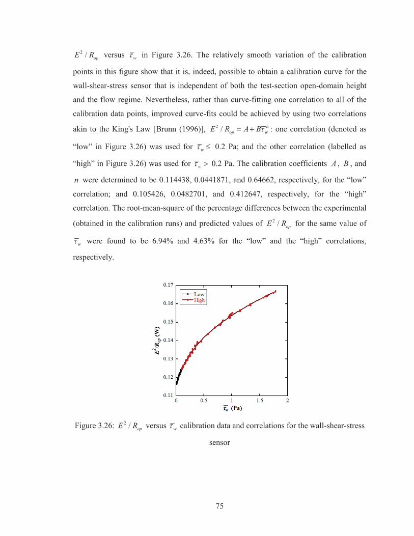
75
2 / opE R versus w in Figure 3.26. The relatively smooth variation of the calibration
points in this figure show that it is, indeed, possible to obtain a calibration curve for the
wall-shear-stress sensor that is independent of both the test-section open-domain height
and the flow regime. Nevertheless, rather than curve-fitting one correlation to all of the
calibration data points, improved curve-fits could be achieved by using two correlations
akin to the King's Law [Brunn (1996)], 2 / nop wE R A B : one correlation (denoted as
“low” in Figure 3.26) was used for w 0.2 Pa; and the other correlation (labelled as
“high” in Figure 3.26) was used for w 0.2 Pa. The calibration coefficients A , B , and
n were determined to be 0.114438, 0.0441871, and 0.64662, respectively, for the “low”
correlation; and 0.105426, 0.0482701, and 0.412647, respectively, for the “high”
correlation. The root-mean-square of the percentage differences between the experimental
(obtained in the calibration runs) and predicted values of 2 / opE R for the same value of
w were found to be 6.94% and 4.63% for the “low” and the “high” correlations,
respectively.
Figure 3.26: 2 / opE R versus w calibration data and correlations for the wall-shear-stress
sensor
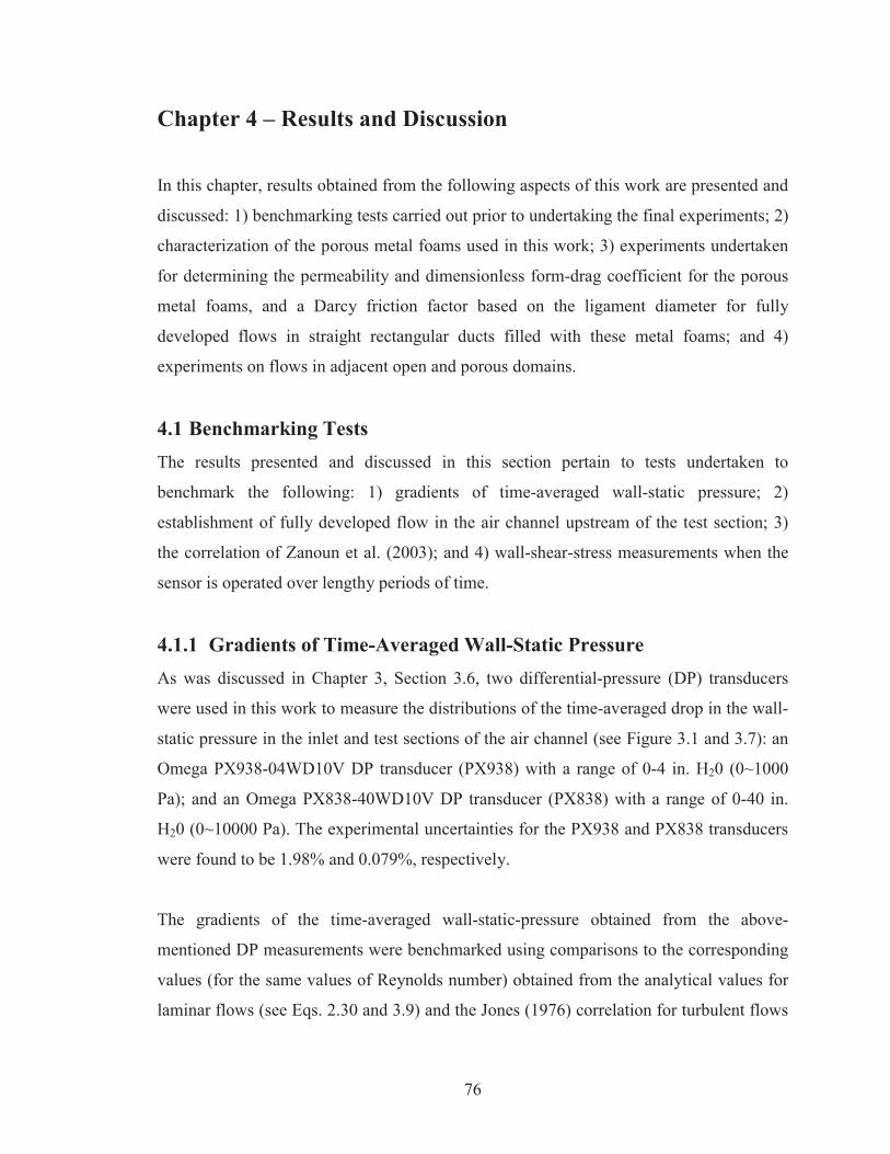
76
Chapter 4 – Results and Discussion
In this chapter, results obtained from the following aspects of this work are presented and
discussed: 1) benchmarking tests carried out prior to undertaking the final experiments; 2)
characterization of the porous metal foams used in this work; 3) experiments undertaken
for determining the permeability and dimensionless form-drag coefficient for the porous
metal foams, and a Darcy friction factor based on the ligament diameter for fully
developed flows in straight rectangular ducts filled with these metal foams; and 4)
experiments on flows in adjacent open and porous domains.
4.1 Benchmarking Tests The results presented and discussed in this section pertain to tests undertaken to
benchmark the following: 1) gradients of time-averaged wall-static pressure; 2)
establishment of fully developed flow in the air channel upstream of the test section; 3)
the correlation of Zanoun et al. (2003); and 4) wall-shear-stress measurements when the
sensor is operated over lengthy periods of time.
4.1.1 Gradients of Time-Averaged Wall-Static Pressure As was discussed in Chapter 3, Section 3.6, two differential-pressure (DP) transducers
were used in this work to measure the distributions of the time-averaged drop in the wall-
static pressure in the inlet and test sections of the air channel (see Figure 3.1 and 3.7): an
Omega PX938-04WD10V DP transducer (PX938) with a range of 0-4 in. H20 (0~1000
Pa); and an Omega PX838-40WD10V DP transducer (PX838) with a range of 0-40 in.
H20 (0~10000 Pa). The experimental uncertainties for the PX938 and PX838 transducers
were found to be 1.98% and 0.079%, respectively.
The gradients of the time-averaged wall-static-pressure obtained from the above-
mentioned DP measurements were benchmarked using comparisons to the corresponding
values (for the same values of Reynolds number) obtained from the analytical values for
laminar flows (see Eqs. 2.30 and 3.9) and the Jones (1976) correlation for turbulent flows
77
(see Eq. 2.33). For laminar flows, the following results were obtained in these
benchmarking tests: the average absolute percentage difference between the values of the
corresponding measured and analytical pressure gradients was 8.34%; the highest of these
values (as high as 19.56%) pertained to two data points obtained with the air channel
configured to the nominal height of 1/2" (see Table 3.2), for which the DPs measured
were of the order of 0.2-0.5 Pa and the accuracy of PX938 DP transducer was quite poor;
exclusion of these two data points brought the average absolute percent difference down
to 3.96%, which was comparable to the uncertainty associated with the values of the
experimentally determined mass flow rate (used in the calculation of the values of the
analytical pressure gradient). For the turbulent flows, the benchmarking tests yielded the
following results: the average absolute percentage difference between the values of the
corresponding pressure gradients obtained from the measurements and the correlation of
Jones (1973) was 13.21%, which is higher than the ±5% uncertainty associated with this
correlation. This higher percentage difference is caused by a contribution to it by the
uncertainty associated with the gap (open-domain) height of the calibration c-channel
(discussed earlier in Chapter 3, Section 3.3.2).
4.1.2 Establishment of Fully Developed Flow Upstream of the Test
Section Benchmarking tests were undertaken to ensure this fully developed flow condition was
indeed established, for all configurations of the test section and the full range of Reynolds
number investigated in this work. Sample results of these tests, for the test section of
nominal 1/4" height (see Table 3.2) are presented in Figure 4.1. In this figure, the
essentially linear variations of the measured drop in time-averaged wall-static pressure,
( )refp p p , with the axial coordinate, x, in the inlet section of the air channel (see
Figures 3.1 and 3.7), for the highest values of the Reynolds number considered in both the
laminar ( Re = 1958) and turbulent ( Re = 10870) flow regimes, demonstrate that fully
developed flow was established upstream of the test section. Similar results were obtained
for all other air channel configurations (see Table 3.2). As these results pertain to the
maximum values of the Reynolds number for the laminar and turbulent flows considered,
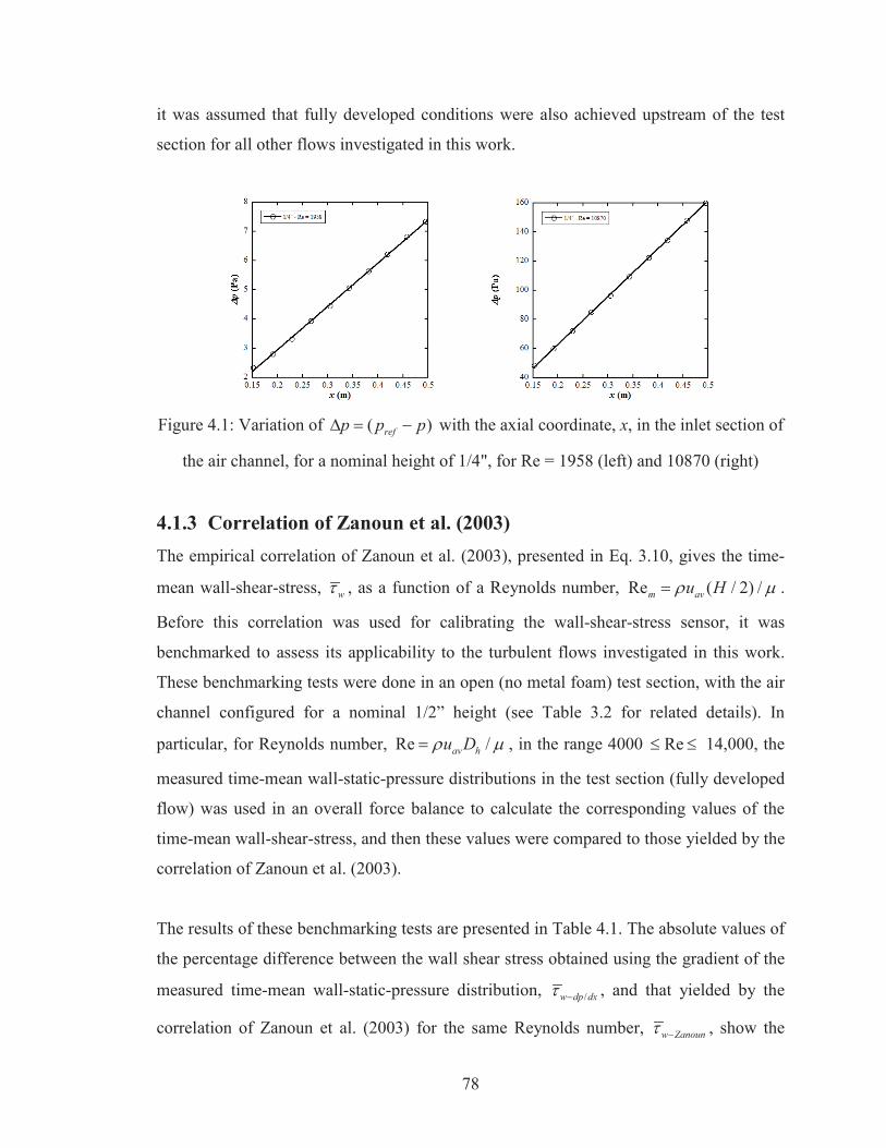
78
it was assumed that fully developed conditions were also achieved upstream of the test
section for all other flows investigated in this work.
Figure 4.1: Variation of ( )refp p p with the axial coordinate, x, in the inlet section of
the air channel, for a nominal height of 1/4", for Re = 1958 (left) and 10870 (right)
4.1.3 Correlation of Zanoun et al. (2003) The empirical correlation of Zanoun et al. (2003), presented in Eq. 3.10, gives the time-
mean wall-shear-stress, w , as a function of a Reynolds number, Re ( / 2) /m avu H .
Before this correlation was used for calibrating the wall-shear-stress sensor, it was
benchmarked to assess its applicability to the turbulent flows investigated in this work.
These benchmarking tests were done in an open (no metal foam) test section, with the air
channel configured for a nominal 1/2” height (see Table 3.2 for related details). In
particular, for Reynolds number, Re /av hu D , in the range 4000 Re 14,000, the
measured time-mean wall-static-pressure distributions in the test section (fully developed
flow) was used in an overall force balance to calculate the corresponding values of the
time-mean wall-shear-stress, and then these values were compared to those yielded by the
correlation of Zanoun et al. (2003).
The results of these benchmarking tests are presented in Table 4.1. The absolute values of
the percentage difference between the wall shear stress obtained using the gradient of the
measured time-mean wall-static-pressure distribution, /w dp dx , and that yielded by the
correlation of Zanoun et al. (2003) for the same Reynolds number, w Zanoun , show the
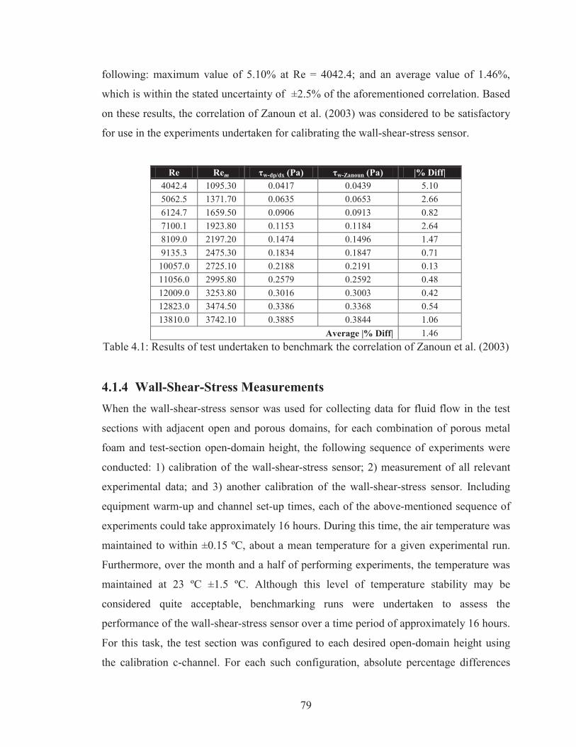
79
following: maximum value of 5.10% at Re = 4042.4; and an average value of 1.46%,
which is within the stated uncertainty of ±2.5% of the aforementioned correlation. Based
on these results, the correlation of Zanoun et al. (2003) was considered to be satisfactory
for use in the experiments undertaken for calibrating the wall-shear-stress sensor.
Re Rem w-dp/dx (Pa) w-Zanoun (Pa) |% Diff| 4042.4 1095.30 0.0417 0.0439 5.10 5062.5 1371.70 0.0635 0.0653 2.66 6124.7 1659.50 0.0906 0.0913 0.82 7100.1 1923.80 0.1153 0.1184 2.64 8109.0 2197.20 0.1474 0.1496 1.47 9135.3 2475.30 0.1834 0.1847 0.71
10057.0 2725.10 0.2188 0.2191 0.13 11056.0 2995.80 0.2579 0.2592 0.48 12009.0 3253.80 0.3016 0.3003 0.42 12823.0 3474.50 0.3386 0.3368 0.54 13810.0 3742.10 0.3885 0.3844 1.06
Average |% Diff| 1.46 Table 4.1: Results of test undertaken to benchmark the correlation of Zanoun et al. (2003)
4.1.4 Wall-Shear-Stress Measurements When the wall-shear-stress sensor was used for collecting data for fluid flow in the test
sections with adjacent open and porous domains, for each combination of porous metal
foam and test-section open-domain height, the following sequence of experiments were
conducted: 1) calibration of the wall-shear-stress sensor; 2) measurement of all relevant
experimental data; and 3) another calibration of the wall-shear-stress sensor. Including
equipment warm-up and channel set-up times, each of the above-mentioned sequence of
experiments could take approximately 16 hours. During this time, the air temperature was
maintained to within ±0.15 ºC, about a mean temperature for a given experimental run.
Furthermore, over the month and a half of performing experiments, the temperature was
maintained at 23 ºC ±1.5 ºC. Although this level of temperature stability may be
considered quite acceptable, benchmarking runs were undertaken to assess the
performance of the wall-shear-stress sensor over a time period of approximately 16 hours.
For this task, the test section was configured to each desired open-domain height using
the calibration c-channel. For each such configuration, absolute percentage differences
80
between the measured time-averaged wall-shear-stress values obtained using the sensor
over the full range of values of the Reynolds number and the corresponding values
yielded by the analytical solution, for laminar flows, and the Zanoun et al. (2003)
correlation, for turbulent flows, were examined.
For laminar flows, the above-mentioned percentage difference could be as high as
18.16% when data from two laminar-flow runs for the nominal open-domain height of
1/2" were included; however, if the data from the two aforementioned laminar-flow runs
were excluded, the average percentage difference reduced to 7.27%, which is comparable
to the 6.94% uncertainty in the ‘low’ calibration curve of the wall-shear-stress sensor (see
Subsection 3.9.5). In this context, it should be noted that in all of the laminar-flow
benchmarking runs, values of the wall shear stress were all below 0.2 Pa and fell within
the ‘low’ calibration range. It should also be noted that large absolute percentage
differences were found, as high as 26.17%, for wall-shear-stress values below 0.02 Pa.
For turbulent flows, the average value of the above-mentioned percentage difference over
all benchmarking runs was 4.03%, which is within the uncertainties of 6.94% and 4.63%
associated with the ‘low’ or ‘high’ calibration curves, respectively, for the wall-shear-
stress sensor (see Subsection 3.9.5). The highest value of the above-mentioned percent
difference for all turbulent-flow benchmarking runs was 13.46%. These results of the
benchmarking runs were considered as confirmation that the wall-shear-stress sensor
performed satisfactorily (within its stated uncertainty) over the above-mentioned 16-hour
time periods, except when very low wall-shear-stress values ( 0.02 Pa) were measured.
4.2 Metal-Foam Characterization In this section, the results of the experiments undertaken to determine the geometrical
aspects and the porosity of the porous metal foams used in this work are presented.
4.2.1 Geometric Aspects The measured values of the following geometric dimensions of the test-section c-channels
with the porous metal foams (see Figure 3.9) are summarized in Table 4.2: open-domain
height, H ; metal-foam-domain height, 1 H ; and channel width, channelW . All
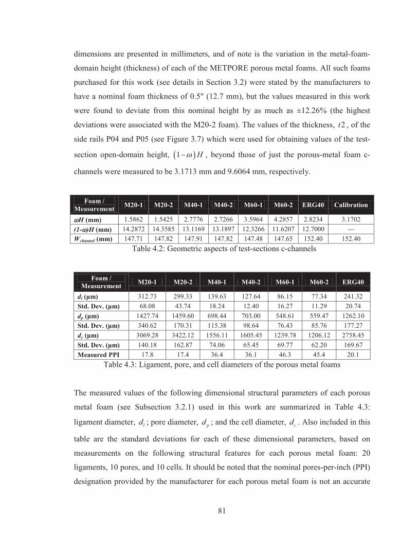
81
dimensions are presented in millimeters, and of note is the variation in the metal-foam-
domain height (thickness) of each of the METPORE porous metal foams. All such foams
purchased for this work (see details in Section 3.2) were stated by the manufacturers to
have a nominal foam thickness of 0.5" (12.7 mm), but the values measured in this work
were found to deviate from this nominal height by as much as ±12.26% (the highest
deviations were associated with the M20-2 foam). The values of the thickness, 2t , of the
side rails P04 and P05 (see Figure 3.7) which were used for obtaining values of the test-
section open-domain height, 1 H , beyond those of just the porous-metal foam c-
channels were measured to be 3.1713 mm and 9.6064 mm, respectively.
Foam / Measurement M20-1 M20-2 M40-1 M40-2 M60-1 M60-2 ERG40 Calibration
H (mm) 1.5862 1.5425 2.7776 2.7266 3.5964 4.2857 2.8234 3.1702 (1- )H (mm) 14.2872 14.3585 13.1169 13.1897 12.3266 11.6207 12.7000 --- Wchannel (mm) 147.71 147.82 147.91 147.82 147.48 147.65 152.40 152.40
Table 4.2: Geometric aspects of test-sections c-channels
Foam / Measurement M20-1 M20-2 M40-1 M40-2 M60-1 M60-2 ERG40
dl 312.73 299.33 139.63 127.64 86.15 77.34 241.32 68.08 43.74 18.24 12.40 16.27 11.29 20.74
dp 1427.74 1459.60 698.44 703.00 548.61 559.47 1262.10 340.62 170.31 115.38 98.64 76.43 85.76 177.27
dc 3069.28 3422.12 1556.11 1605.45 1239.78 1206.12 2758.45 140.18 162.87 74.06 65.45 69.77 62.20 169.67
Measured PPI 17.8 17.4 36.4 36.1 46.3 45.4 20.1 Table 4.3: Ligament, pore, and cell diameters of the porous metal foams
The measured values of the following dimensional structural parameters of each porous
metal foam (see Subsection 3.2.1) used in this work are summarized in Table 4.3:
ligament diameter, ld ; pore diameter, pd ; and the cell diameter, cd . Also included in this
table are the standard deviations for each of these dimensional parameters, based on
measurements on the following structural features for each porous metal foam: 20
ligaments, 10 pores, and 10 cells. It should be noted that the nominal pores-per-inch (PPI)
designation provided by the manufacturer for each porous metal foam is not an accurate
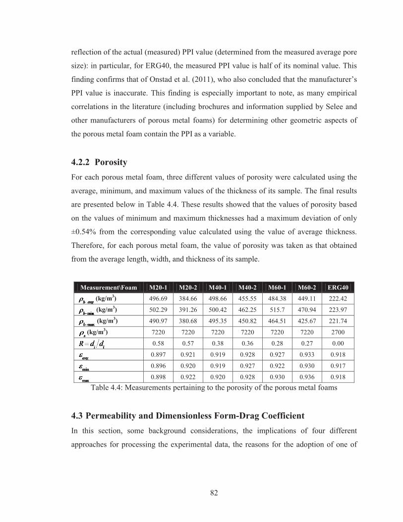
82
reflection of the actual (measured) PPI value (determined from the measured average pore
size): in particular, for ERG40, the measured PPI value is half of its nominal value. This
finding confirms that of Onstad et al. (2011), who also concluded that the manufacturer’s
PPI value is inaccurate. This finding is especially important to note, as many empirical
correlations in the literature (including brochures and information supplied by Selee and
other manufacturers of porous metal foams) for determining other geometric aspects of
the porous metal foam contain the PPI as a variable.
4.2.2 Porosity For each porous metal foam, three different values of porosity were calculated using the
average, minimum, and maximum values of the thickness of its sample. The final results
are presented below in Table 4.4. These results showed that the values of porosity based
on the values of minimum and maximum thicknesses had a maximum deviation of only
±0.54% from the corresponding value calculated using the value of average thickness.
Therefore, for each porous metal foam, the value of porosity was taken as that obtained
from the average length, width, and thickness of its sample.
Measurement\Foam M20-1 M20-2 M40-1 M40-2 M60-1 M60-2 ERG40
(kg/m3) 496.69 384.66 498.66 455.55 484.38 449.11 222.42
(kg/m3) 502.29 391.26 500.42 462.25 515.7 470.94 223.97
(kg/m3) 490.97 380.68 495.35 450.82 464.51 425.67 221.74
(kg/m3) 7220 7220 7220 7220 7220 7220 2700
0.58 0.57 0.38 0.36 0.28 0.27 0.00
0.897 0.921 0.919 0.928 0.927 0.933 0.918
0.896 0.920 0.919 0.927 0.922 0.930 0.917
0.898 0.922 0.920 0.928 0.930 0.936 0.918
Table 4.4: Measurements pertaining to the porosity of the porous metal foams
4.3 Permeability and Dimensionless Form-Drag Coefficient In this section, some background considerations, the implications of four different
approaches for processing the experimental data, the reasons for the adoption of one of
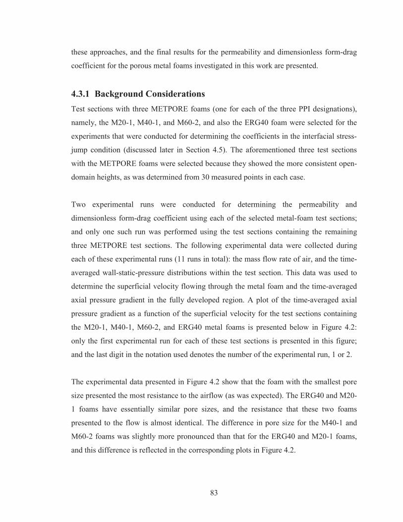
83
these approaches, and the final results for the permeability and dimensionless form-drag
coefficient for the porous metal foams investigated in this work are presented.
4.3.1 Background Considerations Test sections with three METPORE foams (one for each of the three PPI designations),
namely, the M20-1, M40-1, and M60-2, and also the ERG40 foam were selected for the
experiments that were conducted for determining the coefficients in the interfacial stress-
jump condition (discussed later in Section 4.5). The aforementioned three test sections
with the METPORE foams were selected because they showed the more consistent open-
domain heights, as was determined from 30 measured points in each case.
Two experimental runs were conducted for determining the permeability and
dimensionless form-drag coefficient using each of the selected metal-foam test sections;
and only one such run was performed using the test sections containing the remaining
three METPORE test sections. The following experimental data were collected during
each of these experimental runs (11 runs in total): the mass flow rate of air, and the time-
averaged wall-static-pressure distributions within the test section. This data was used to
determine the superficial velocity flowing through the metal foam and the time-averaged
axial pressure gradient in the fully developed region. A plot of the time-averaged axial
pressure gradient as a function of the superficial velocity for the test sections containing
the M20-1, M40-1, M60-2, and ERG40 metal foams is presented below in Figure 4.2:
only the first experimental run for each of these test sections is presented in this figure;
and the last digit in the notation used denotes the number of the experimental run, 1 or 2.
The experimental data presented in Figure 4.2 show that the foam with the smallest pore
size presented the most resistance to the airflow (as was expected). The ERG40 and M20-
1 foams have essentially similar pore sizes, and the resistance that these two foams
presented to the flow is almost identical. The difference in pore size for the M40-1 and
M60-2 foams was slightly more pronounced than that for the ERG40 and M20-1 foams,
and this difference is reflected in the corresponding plots in Figure 4.2.
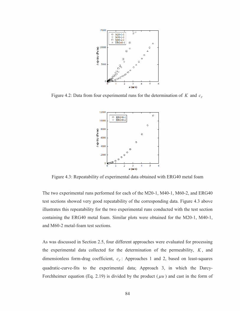
84
Figure 4.2: Data from four experimental runs for the determination of K and Fc
Figure 4.3: Repeatability of experimental data obtained with ERG40 metal foam
The two experimental runs performed for each of the M20-1, M40-1, M60-2, and ERG40
test sections showed very good repeatability of the corresponding data. Figure 4.3 above
illustrates this repeatability for the two experimental runs conducted with the test section
containing the ERG40 metal foam. Similar plots were obtained for the M20-1, M40-1,
and M60-2 metal-foam test sections.
As was discussed in Section 2.5, four different approaches were evaluated for processing
the experimental data collected for the determination of the permeability, K , and
dimensionless form-drag coefficient, Fc : Approaches 1 and 2, based on least-squares
quadratic-curve-fits to the experimental data; Approach 3, in which the Darcy-
Forchheimer equation (Eq. 2.19) is divided by the product ( u ) and cast in the form of
85
Eq. 2.22, and a least-squares linear-curve-fit to experimentally determined values of the
terms in this latter equation; and Approach 4, in which the experimental data that falls in
the so-called Darcy regime (form-drag or Forchheimer term is ignored in this regime) is
processed first using a least-squares linear-curve-fit to determine the value of K , and
then this value of permeability and all experimental data points are used in a least-squares
quadratic-curve-fit to determine the value of Fc . The results obtained with Approaches 1
and 2 are discussed next in Subsection 4.3.2; then, in Section 4.3.3, the results obtained
with Approach 4 are discussed; the results obtained with Approach 3, the approach finally
adopted in this work, are presented in Subsection 4.3.4; and in Subsection 4.3.5, the final
results for K and Fc are presented and discussed.
4.3.2 Approaches 1 and 2 Taking the data obtained for the experiments conducted with the ERG40-1 metal foam as
an example, the following results were obtained: permeability values of 5.1087E-08 m2
and 5.4822E-08 m2 with Approaches 1 and 2, respectively (an absolute percentage
difference of 7.05%); and dimensionless form-drag coefficient values of 0.06449 and
0.06911 with Approaches 1 and 2, respectively (an absolute percentage difference of
6.92%). The curve-fits in both these approaches produced excellent coefficients of
determination, 0.99994 and 0.99998 for Approaches 1 and 2, respectively. These results,
and similar results obtained with the experimental data obtained with the other metal
foams investigated in this work, show that there is an appreciable difference in the values
of K and Fc yielded by the Approaches 1 and 2. To further assess these two approaches,
the percentage difference between the experimental values of the pressure gradient in the
test sections with the different foams and those calculated using the values of values of K
and Fc yielded by each of the Approaches 1 and 2 were examined. Based on an
examination of the average values of these percentage differences over all data points
obtained in the ERG40-1 run, Approach 2 outperformed Approach 1, yielding values of
9.17% and 12.61%, respectively. Similar results were obtained with the data from
experimental runs with the other metal foams. The results obtained with these two
approaches are compared to those obtained with Approach 3 in Subsection 4.3.4.
86
4.3.3 Approach 4
In this approach, first, tentative values of K and Fc are determined using the above-
mentioned Approach 2; then, these values are used to assess the contribution of the
Forchheimer term to the axial pressure gradient for each experimental data point. Using
this approach, it was determined that for the M60 metal foam, for a few of the data points,
the contribution of the Forchheimer term to the axial pressure gradient was as low as 1%;
however, for the other metal foams investigated in this work, the limit on this contribution
had to be set to about 15% to ensure enough data points for a statistically meaningful
calculation of the value of K .
Using the above-mentioned technique for the demarcation of the Darcy regime, Approach
4, and the experimental data obtained for the M60 metal foam, the permeability was
determined to be 1.0510E-08 m2 and 9.6687E-09 m2 when the above-mentioned limit was
set to 5% and 15%, respectively (a percent difference of 8.34%); and the dimensionless
form-drag coefficient was determined to be 0.09482 and 0.07964 with the 5% and 15%
limits, respectively (a percent difference of 10.58%). These percentage differences were
considered too high, so it was concluded that a 15% limit for the contribution of the
Forchheimer term to the axial pressure gradient would not produce reliable results for the
values of K and Fc . It may be practical and viable to fix this limit at 5% or even lower.
However, with the experimental apparatus and instrumentation used in this work, for
conditions corresponding to limits lower than 5%, it was not possible to measure the mass
flow rates and the pressure drops with sufficient accuracy, so Approach 4 was not
applicable. Nevertheless, although this approach was not applicable in this work, the
author still believes it is worthy of further investigation, possibly in future works with the
incorporation of LFEs with smaller tubes and a differential-pressure transducer capable of
accurately measuring values of 10 Pa or lower (and related calibration capability).
4.3.4 Approach 3 For convenience in the presentation, Eq. 2.22 is repeated below, and the data pertaining to
the ERG40-1 run is presented in Figure 4.4:
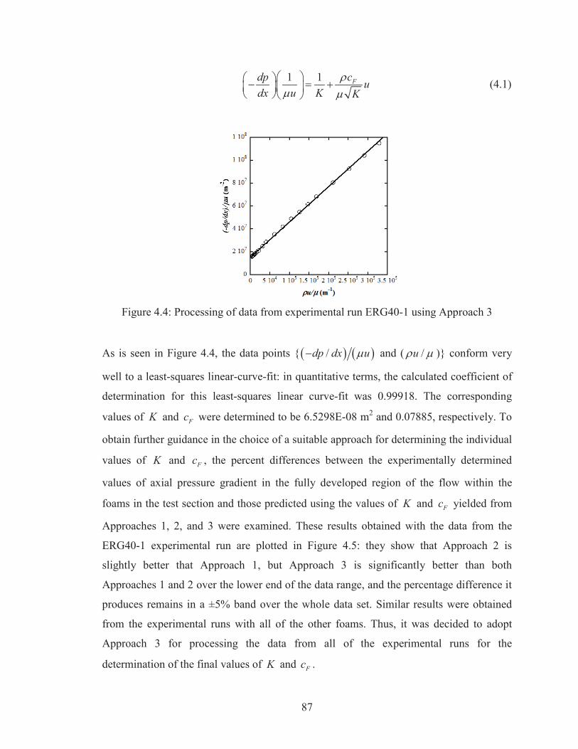
87
1 1 Fcdp udx u K K
(4.1)
Figure 4.4: Processing of data from experimental run ERG40-1 using Approach 3
As is seen in Figure 4.4, the data points { /dp dx u and ( /u )} conform very
well to a least-squares linear-curve-fit: in quantitative terms, the calculated coefficient of
determination for this least-squares linear curve-fit was 0.99918. The corresponding
values of K and Fc were determined to be 6.5298E-08 m2 and 0.07885, respectively. To
obtain further guidance in the choice of a suitable approach for determining the individual
values of K and Fc , the percent differences between the experimentally determined
values of axial pressure gradient in the fully developed region of the flow within the
foams in the test section and those predicted using the values of K and Fc yielded from
Approaches 1, 2, and 3 were examined. These results obtained with the data from the
ERG40-1 experimental run are plotted in Figure 4.5: they show that Approach 2 is
slightly better that Approach 1, but Approach 3 is significantly better than both
Approaches 1 and 2 over the lower end of the data range, and the percentage difference it
produces remains in a ±5% band over the whole data set. Similar results were obtained
from the experimental runs with all of the other foams. Thus, it was decided to adopt
Approach 3 for processing the data from all of the experimental runs for the
determination of the final values of K and Fc .
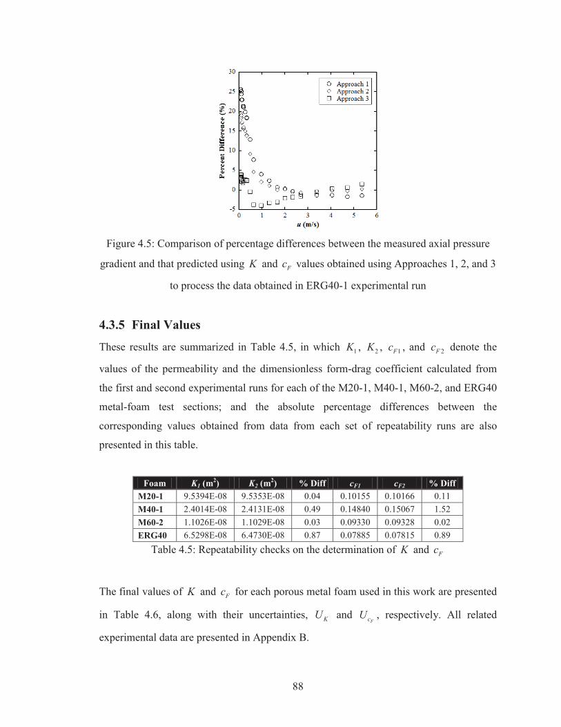
88
Figure 4.5: Comparison of percentage differences between the measured axial pressure
gradient and that predicted using K and Fc values obtained using Approaches 1, 2, and 3
to process the data obtained in ERG40-1 experimental run
4.3.5 Final Values
These results are summarized in Table 4.5, in which 1K , 2K , 1Fc , and 2Fc denote the
values of the permeability and the dimensionless form-drag coefficient calculated from
the first and second experimental runs for each of the M20-1, M40-1, M60-2, and ERG40
metal-foam test sections; and the absolute percentage differences between the
corresponding values obtained from data from each set of repeatability runs are also
presented in this table.
Foam K1 (m2) K2 (m2) % Diff cF1 cF2 % Diff M20-1 9.5394E-08 9.5353E-08 0.04 0.10155 0.10166 0.11 M40-1 2.4014E-08 2.4131E-08 0.49 0.14840 0.15067 1.52 M60-2 1.1026E-08 1.1029E-08 0.03 0.09330 0.09328 0.02 ERG40 6.5298E-08 6.4730E-08 0.87 0.07885 0.07815 0.89
Table 4.5: Repeatability checks on the determination of K and Fc
The final values of K and Fc for each porous metal foam used in this work are presented
in Table 4.6, along with their uncertainties, KU and FcU , respectively. All related
experimental data are presented in Appendix B.
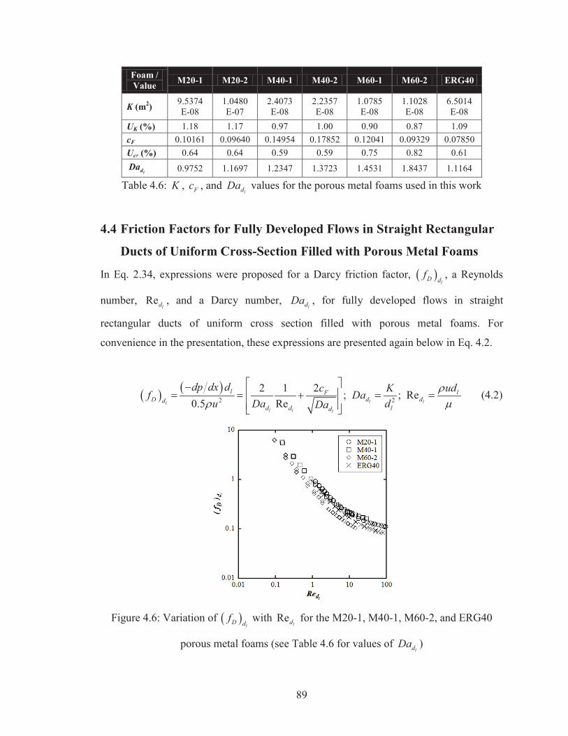
89
Foam / Value M20-1 M20-2 M40-1 M40-2 M60-1 M60-2 ERG40
K (m2) 9.5374 E-08
1.0480 E-07
2.4073 E-08
2.2357 E-08
1.0785 E-08
1.1028 E-08
6.5014 E-08
UK (%) 1.18 1.17 0.97 1.00 0.90 0.87 1.09 cF 0.10161 0.09640 0.14954 0.17852 0.12041 0.09329 0.07850 UcF (%) 0.64 0.64 0.59 0.59 0.75 0.82 0.61
ldDa 0.9752 1.1697 1.2347 1.3723 1.4531 1.8437 1.1164
Table 4.6: K , Fc , and ldDa values for the porous metal foams used in this work
4.4 Friction Factors for Fully Developed Flows in Straight Rectangular
Ducts of Uniform Cross-Section Filled with Porous Metal Foams
In Eq. 2.34, expressions were proposed for a Darcy friction factor, l
D df , a Reynolds
number, Reld , and a Darcy number,
ldDa , for fully developed flows in straight
rectangular ducts of uniform cross section filled with porous metal foams. For
convenience in the presentation, these expressions are presented again below in Eq. 4.2.
2 2
22 1 ; ; Re0.5 Re l ll
l l l
l lFD d dd
d d ld
dp dx d udc Kf Dau Da dDa
(4.2)
Figure 4.6: Variation of l
D df with Re
ld for the M20-1, M40-1, M60-2, and ERG40
porous metal foams (see Table 4.6 for values of ldDa )
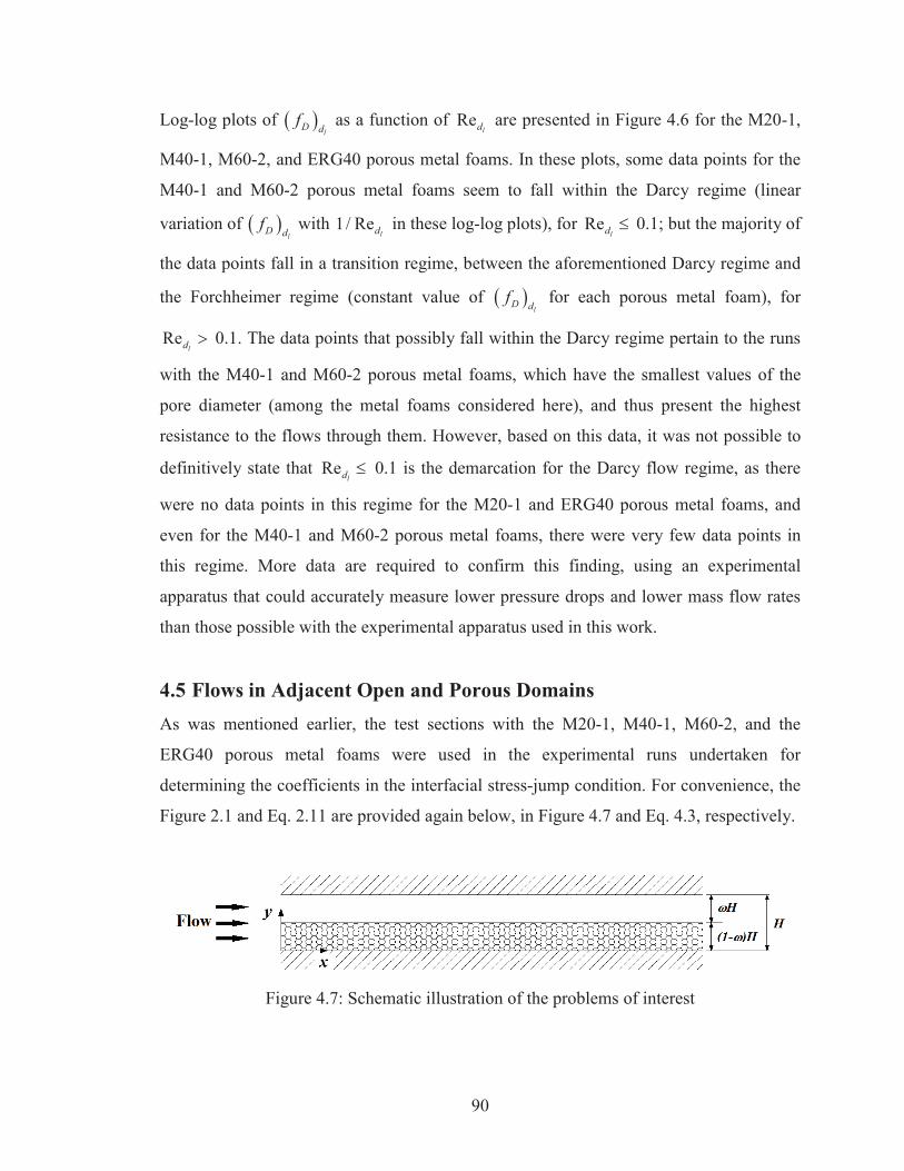
90
Log-log plots of l
D df as a function of Re
ld are presented in Figure 4.6 for the M20-1,
M40-1, M60-2, and ERG40 porous metal foams. In these plots, some data points for the
M40-1 and M60-2 porous metal foams seem to fall within the Darcy regime (linear
variation of l
D df with 1/ Re
ld in these log-log plots), for Reld 0.1; but the majority of
the data points fall in a transition regime, between the aforementioned Darcy regime and
the Forchheimer regime (constant value of l
D df for each porous metal foam), for
Reld 0.1. The data points that possibly fall within the Darcy regime pertain to the runs
with the M40-1 and M60-2 porous metal foams, which have the smallest values of the
pore diameter (among the metal foams considered here), and thus present the highest
resistance to the flows through them. However, based on this data, it was not possible to
definitively state that Reld 0.1 is the demarcation for the Darcy flow regime, as there
were no data points in this regime for the M20-1 and ERG40 porous metal foams, and
even for the M40-1 and M60-2 porous metal foams, there were very few data points in
this regime. More data are required to confirm this finding, using an experimental
apparatus that could accurately measure lower pressure drops and lower mass flow rates
than those possible with the experimental apparatus used in this work.
4.5 Flows in Adjacent Open and Porous Domains As was mentioned earlier, the test sections with the M20-1, M40-1, M60-2, and the
ERG40 porous metal foams were used in the experimental runs undertaken for
determining the coefficients in the interfacial stress-jump condition. For convenience, the
Figure 2.1 and Eq. 2.11 are provided again below, in Figure 4.7 and Eq. 4.3, respectively.
Figure 4.7: Schematic illustration of the problems of interest
91
2* *1 * 2 *
* *
1 1 ReI I
pd od
du du u udy dy Da
(4.3)
The various dimensionless variables that appear in this equation were defined and
discussed in Sections 2.3 and 2.4, so they are not repeated here.
The following data were collected in the experiments on fully developed fluid flows in
test sections with adjacent open and porous domains, and some of the data that
corresponded to the laminar-flow regime were used for determining the coefficients in the
interfacial stress-jump condition: the total mass flow rate of air flowing through the test
section, totalm ; the absolute temperature, dynamic viscosity, and density of air within the
test section, absT , , and , respectively; and axial variation of the time-averaged wall-
static-pressure drop along the top wall and the instantaneous and time-averaged values of
wall-shear-stress at one location on the top wall. The full sets of experimental data
collected in these experiments could be useful in validating and refining mathematical
models of transitional and turbulent flows in the problems of interest, and are a key
contribution of this work; these data are concisely presented in Appendix C. These data,
along with the analytical solution for laminar flows and related physical requirements (as
presented in Section 2.4) were used to obtain the following results: open-domain
interfacial shear stress; open- and porous-domain interfacial dimensionless velocity
gradients (normal to the interface) for laminar flow; guidance for laminar-turbulent
transition in the flows of interest; the coefficients in the interfacial tangential stress-jump
condition; and the open-domain Darcy friction factor. These results are presented and
discussed in the following subsections.
4.5.1 Open-Domain Interfacial Shear Stress As was discussed in Section 2.4, the open-domain interfacial shear stress can be
calculated using the following equation, obtained using a simple force balance on the
open-domain side of the problem of interest, and the measured wall-shear-stress values on
the surface of the top wall:
92
I UWod oddp dx H (4.4)
As was noted in Chapter 2, this equation applies to laminar flow and also turbulent flow
(if the shear stresses and pressure gradient are interpreted as time-averaged quantities).
4.5.2 Open- and Porous-Domain Interfacial Dimensionless Velocity
Gradients (Normal to the Interface) in Laminar Flow The open-domain interfacial wall shear stress and the analytical solution to laminar flow
in the problems of interest were used to determine the above-mentioned dimensionless
velocity gradients, using Eq. 2.17, which is repeated below for convenience:
2*
* * *
* 1** * 3
[0.5 /{( / ) }]
( / ) [0.5 ( / )]4( )( / ) (1 )
(1 )
I Iod
I Iod
Ipd
u dp dx H
du dy uu udu dy C CB
C
(4.5)
The various dimensional and dimensionless variables that appear in these equations were
defined and discussed in Section 2.4, so they are not repeated here. As was noted above,
the solution given in Eq. 4.5 applies only to laminar flows. Thus, when using this
solution, it is necessary to determine which data points obtained in the related
experiments pertain to the laminar-flow regime. Guidance for this determination required
special considerations, which are discussed in the next subsection.
4.5.3 Guidance for Determining Laminar-Turbulent Transition Guidance for determining laminar-turbulent transition in the problems of interest was
obtained using several indicators. First, it must be realized that only two physically
tenable shapes exist for the laminar-flow velocity profiles: in one, the interfacial velocity
exceeds the superficial velocity within the porous domain; in the other, the interfacial
velocity is less than the superficial velocity within the porous domain; and qualitative
sketches of these two physically tenable shapes are given in the figure below.
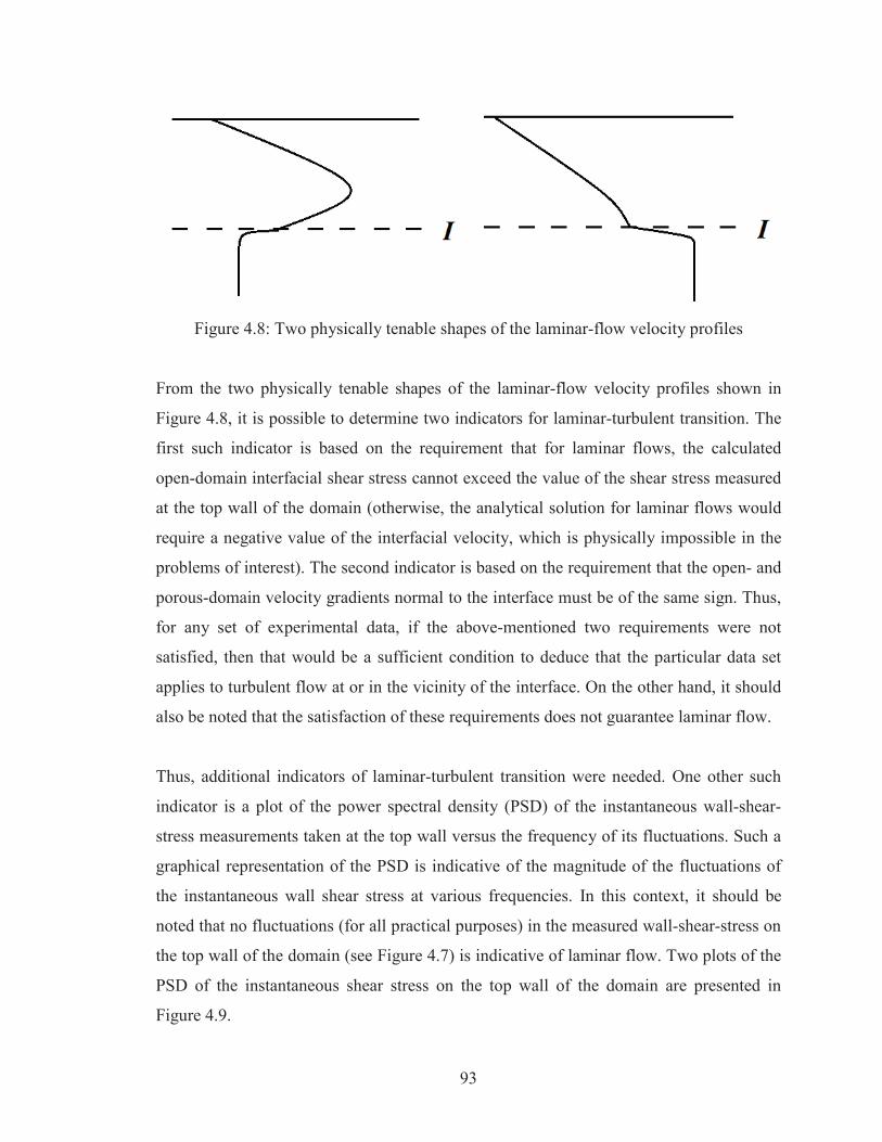
93
Figure 4.8: Two physically tenable shapes of the laminar-flow velocity profiles
From the two physically tenable shapes of the laminar-flow velocity profiles shown in
Figure 4.8, it is possible to determine two indicators for laminar-turbulent transition. The
first such indicator is based on the requirement that for laminar flows, the calculated
open-domain interfacial shear stress cannot exceed the value of the shear stress measured
at the top wall of the domain (otherwise, the analytical solution for laminar flows would
require a negative value of the interfacial velocity, which is physically impossible in the
problems of interest). The second indicator is based on the requirement that the open- and
porous-domain velocity gradients normal to the interface must be of the same sign. Thus,
for any set of experimental data, if the above-mentioned two requirements were not
satisfied, then that would be a sufficient condition to deduce that the particular data set
applies to turbulent flow at or in the vicinity of the interface. On the other hand, it should
also be noted that the satisfaction of these requirements does not guarantee laminar flow.
Thus, additional indicators of laminar-turbulent transition were needed. One other such
indicator is a plot of the power spectral density (PSD) of the instantaneous wall-shear-
stress measurements taken at the top wall versus the frequency of its fluctuations. Such a
graphical representation of the PSD is indicative of the magnitude of the fluctuations of
the instantaneous wall shear stress at various frequencies. In this context, it should be
noted that no fluctuations (for all practical purposes) in the measured wall-shear-stress on
the top wall of the domain (see Figure 4.7) is indicative of laminar flow. Two plots of the
PSD of the instantaneous shear stress on the top wall of the domain are presented in
Figure 4.9.
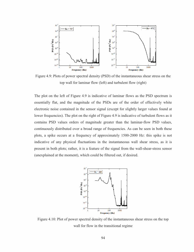
94
Figure 4.9: Plots of power spectral density (PSD) of the instantaneous shear stress on the
top wall for laminar flow (left) and turbulent flow (right)
The plot on the left of Figure 4.9 is indicative of laminar flows as the PSD spectrum is
essentially flat, and the magnitude of the PSDs are of the order of effectively white
electronic noise contained in the sensor signal (except for slightly larger values found at
lower frequencies). The plot on the right of Figure 4.9 is indicative of turbulent flows as it
contains PSD values orders of magnitude greater than the laminar-flow PSD values,
continuously distributed over a broad range of frequencies. As can be seen in both these
plots, a spike occurs at a frequency of approximately 1500-2000 Hz: this spike is not
indicative of any physical fluctuations in the instantaneous wall shear stress, as it is
present in both plots; rather, it is a feature of the signal from the wall-shear-stress sensor
(unexplained at the moment), which could be filtered out, if desired.
Figure 4.10: Plot of power spectral density of the instantaneous shear stress on the top
wall for flow in the transitional regime
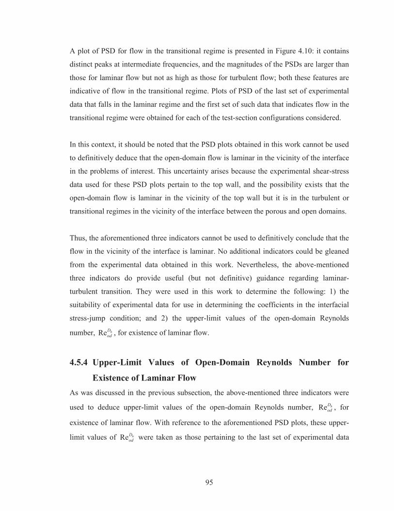
95
A plot of PSD for flow in the transitional regime is presented in Figure 4.10: it contains
distinct peaks at intermediate frequencies, and the magnitudes of the PSDs are larger than
those for laminar flow but not as high as those for turbulent flow; both these features are
indicative of flow in the transitional regime. Plots of PSD of the last set of experimental
data that falls in the laminar regime and the first set of such data that indicates flow in the
transitional regime were obtained for each of the test-section configurations considered.
In this context, it should be noted that the PSD plots obtained in this work cannot be used
to definitively deduce that the open-domain flow is laminar in the vicinity of the interface
in the problems of interest. This uncertainty arises because the experimental shear-stress
data used for these PSD plots pertain to the top wall, and the possibility exists that the
open-domain flow is laminar in the vicinity of the top wall but it is in the turbulent or
transitional regimes in the vicinity of the interface between the porous and open domains.
Thus, the aforementioned three indicators cannot be used to definitively conclude that the
flow in the vicinity of the interface is laminar. No additional indicators could be gleaned
from the experimental data obtained in this work. Nevertheless, the above-mentioned
three indicators do provide useful (but not definitive) guidance regarding laminar-
turbulent transition. They were used in this work to determine the following: 1) the
suitability of experimental data for use in determining the coefficients in the interfacial
stress-jump condition; and 2) the upper-limit values of the open-domain Reynolds
number, Re hDod , for existence of laminar flow.
4.5.4 Upper-Limit Values of Open-Domain Reynolds Number for
Existence of Laminar Flow As was discussed in the previous subsection, the above-mentioned three indicators were
used to deduce upper-limit values of the open-domain Reynolds number, Re hDod , for
existence of laminar flow. With reference to the aforementioned PSD plots, these upper-
limit values of Re hDod were taken as those pertaining to the last set of experimental data
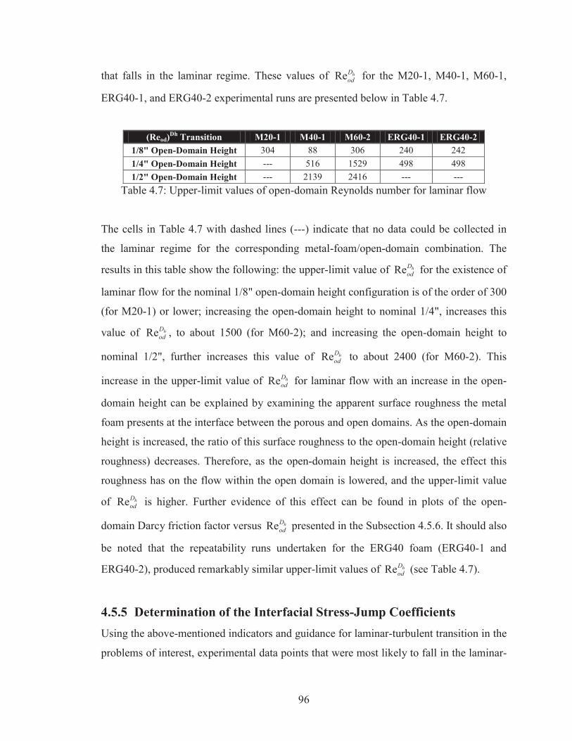
96
that falls in the laminar regime. These values of Re hDod for the M20-1, M40-1, M60-1,
ERG40-1, and ERG40-2 experimental runs are presented below in Table 4.7.
(Reod)Dh Transition M20-1 M40-1 M60-2 ERG40-1 ERG40-2 1/8" Open-Domain Height 304 88 306 240 242 1/4" Open-Domain Height --- 516 1529 498 498 1/2" Open-Domain Height --- 2139 2416 --- ---
Table 4.7: Upper-limit values of open-domain Reynolds number for laminar flow
The cells in Table 4.7 with dashed lines (---) indicate that no data could be collected in
the laminar regime for the corresponding metal-foam/open-domain combination. The
results in this table show the following: the upper-limit value of Re hDod for the existence of
laminar flow for the nominal 1/8" open-domain height configuration is of the order of 300
(for M20-1) or lower; increasing the open-domain height to nominal 1/4", increases this
value of Re hDod , to about 1500 (for M60-2); and increasing the open-domain height to
nominal 1/2", further increases this value of Re hDod to about 2400 (for M60-2). This
increase in the upper-limit value of Re hDod for laminar flow with an increase in the open-
domain height can be explained by examining the apparent surface roughness the metal
foam presents at the interface between the porous and open domains. As the open-domain
height is increased, the ratio of this surface roughness to the open-domain height (relative
roughness) decreases. Therefore, as the open-domain height is increased, the effect this
roughness has on the flow within the open domain is lowered, and the upper-limit value
of Re hDod is higher. Further evidence of this effect can be found in plots of the open-
domain Darcy friction factor versus Re hDod presented in the Subsection 4.5.6. It should also
be noted that the repeatability runs undertaken for the ERG40 foam (ERG40-1 and
ERG40-2), produced remarkably similar upper-limit values of Re hDod (see Table 4.7).
4.5.5 Determination of the Interfacial Stress-Jump Coefficients Using the above-mentioned indicators and guidance for laminar-turbulent transition in the
problems of interest, experimental data points that were most likely to fall in the laminar-
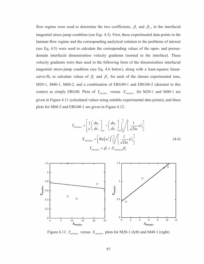
97
flow regime were used to determine the two coefficients, 1 and 2 , in the interfacial
tangential stress-jump condition (see Eqs. 4.3). First, these experimental data points in the
laminar-flow regime and the corresponding analytical solution to the problems of interest
(see Eq. 4.5) were used to calculate the corresponding values of the open- and porous-
domain interfacial dimensionless velocity gradients (normal to the interface). These
velocity gradients were then used in the following form of the dimensionless interfacial
tangential stress-jump condition (see Eq. 4.6 below), along with a least-squares linear-
curve-fit, to calculate values of 1 and 2 for each of the chosen experimental runs,
M20-1, M40-1, M60-2, and a combination of ERG40-1 and ERG40-2 (denoted in this
context as simply ERG40. Plots of interfaceY versus interfaceX for M20-1 and M40-1 are
given in Figure 4.11 (calculated values using suitable experimental data points); and these
plots for M60-2 and ERG40-1 are given in Figure 4.12.
* **
* *
2
* *
1 2
1 1
1Re
I II
interfacepd od
I Iinterface
interface interface
du duY udy dy Da
X u uDa
Y X
(4.6)
Figure 4.11: interfaceY versus interfaceX plots for M20-1 (left) and M40-1 (right)
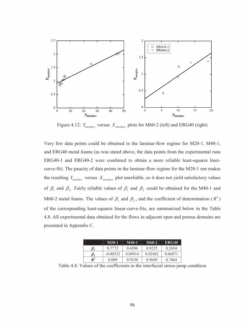
98
Figure 4.12: interfaceY versus interfaceX plots for M60-2 (left) and ERG40 (right)
Very few data points could be obtained in the laminar-flow regime for M20-1, M40-1,
and ERG40 metal foams (as was stated above, the data points from the experimental runs
ERG40-1 and ERG40-2 were combined to obtain a more reliable least-squares liner-
curve-fit). The paucity of data points in the laminar-flow regime for the M20-1 run makes
the resulting interfaceY versus interfaceX plot unreliable, so it does not yield satisfactory values
of 1 and 2 . Fairly reliable values of 1 and 2 could be obtained for the M40-1 and
M60-2 metal foams. The values of 1 and 2 , and the coefficient of determination ( 2R )
of the corresponding least-squares linear-curve-fits, are summarized below in the Table
4.8. All experimental data obtained for the flows in adjacent open and porous domains are
presented in Appendix C.
M20-1 M40-1 M60-2 ERG40 1 0.7772 0.4506 0.9225 0.2654
2 -0.00523 0.09914 0.02482 0.06871 R2 0.009 0.9230 0.9649 0.7464
Table 4.8: Values of the coefficients in the interfacial stress-jump condition
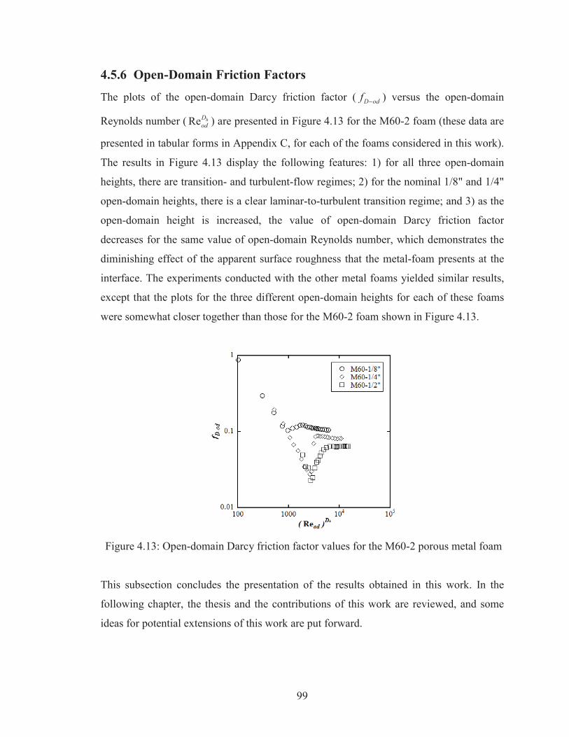
99
4.5.6 Open-Domain Friction Factors
The plots of the open-domain Darcy friction factor ( D odf ) versus the open-domain
Reynolds number ( Re hDod ) are presented in Figure 4.13 for the M60-2 foam (these data are
presented in tabular forms in Appendix C, for each of the foams considered in this work).
The results in Figure 4.13 display the following features: 1) for all three open-domain
heights, there are transition- and turbulent-flow regimes; 2) for the nominal 1/8" and 1/4"
open-domain heights, there is a clear laminar-to-turbulent transition regime; and 3) as the
open-domain height is increased, the value of open-domain Darcy friction factor
decreases for the same value of open-domain Reynolds number, which demonstrates the
diminishing effect of the apparent surface roughness that the metal-foam presents at the
interface. The experiments conducted with the other metal foams yielded similar results,
except that the plots for the three different open-domain heights for each of these foams
were somewhat closer together than those for the M60-2 foam shown in Figure 4.13.
Figure 4.13: Open-domain Darcy friction factor values for the M60-2 porous metal foam
This subsection concludes the presentation of the results obtained in this work. In the
following chapter, the thesis and the contributions of this work are reviewed, and some
ideas for potential extensions of this work are put forward.
100
Chapter 5 – Conclusion
This final chapter contains a review of the thesis, a summary of the contributions of this
work, and some recommendations for extensions of this work.
4.1 Review of the Thesis In Chapter 1, the motivation for this work, its overall goals and specific objectives, a
review of the relevant literature, and the organization of the thesis were presented. Central
to the literature review were discussions of the permeability and dimensionless form-drag
coefficient of porous media, and fluid flows in adjacent open and porous domains. The
practices of using empirical correlations and experimental data for determining the
permeability and dimensionless form-drag coefficient were comparatively discussed, and
their advantages, difficulties, and shortcomings were highlighted. Various approaches to
modeling fluid flows in adjacent open and porous domains were presented. It was
discussed in this context that if the most practical of these approaches (the macroscopic-
scale approach) is used along with the assumption of uniform porosity and permeability
throughout the porous medium, all the way to the interface between the open and porous
domains, then an interfacial condition is needed to account for an apparent jump in the
shear (tangential) stress. This interfacial condition contains two dimensionless
coefficients, of order unity or less. It was also highlighted that experimental inputs are
critically important and urgently needed for the determination of the aforementioned two
dimensionless coefficients in the interfacial tangential stress-jump condition.
The theoretical considerations used in this work for designing the experimental set-ups
and procedures, selecting and implementing related instrumentation, and processing the
experimental data collected were presented and concisely discussed in Chapter 2. The
assumptions invoked and the mathematical models of the problems of interest were
presented. The emphasis was on a macroscopic approach to the mathematical modeling of
Newtonian fluid flows in adjacent open and porous domains: the fluid flow in the open
domain was modeled using the continuity and Navier-Stokes equations; the volume-
averaged forms of the continuity equation and the momentum equation (Darcy-Brinkman-
101
Forchheimer equation) were used to model the fluid flow in the porous domain; the no-
slip and impermeability conditions were imposed at solid boundaries; the velocity
(superficial velocity in the porous domain), pressure (intrinsic-phase-average pressure in
the porous domain), and normal stresses were assumed to be continuous at the interface
between the open and porous domains; and the apparent jump in the shear stress at this
interface was handled using a condition which involved two dimensionless coefficients.
An analytical solution for laminar, fully developed, constant-property Newtonian fluid
flow in the problem of interest was adapted from the works of Kuznetsov (1999) and
Costa et al. (2008). Four different approaches for processing the data obtained from
experiments for determining the permeability and dimensionless form-drag coefficient for
the porous metal foam used in this work were presented, with special emphasis on their
pros and cons. Use of the aforementioned analytical solution and experimental data (for
laminar flows) for the determination of the two coefficients in the interfacial tangential
stress-jump condition was also discussed. Finally, the definitions of several friction
factors were presented along with related analytical solutions (when possible) or
empirical correlations (if available) for laminar and turbulent flows in straight rectangular
ducts with no porous medium (entirely open or unobstructed), completely filled with
porous metal foam, and containing adjacent open and porous-metal-foam domains.
The porous metal foams and the experimental apparatus used in this work (a straight
rectangular air channel, flow-measurement devices, and related instrumentation) were
described in Chapter 3. The air channel was specially designed and constructed to
conveniently allow experiments in which the test section had no porous medium within it
(entirely open), was fully filled with the porous metal foams, and contained adjacent open
and porous-metal-foam domains, with three different open-domain heights. The top wall
of the test section was designed to incorporate 64 wall-static-pressure taps (for the
measurement of time-averaged wall-static-pressure distributions) and also a wall-shear-
stress sensor (for measurements of instantaneous and time-averaged wall-shear-stress)
flush-mounted within a cylindrical Delrin insert. The wall-shear-stress sensor was
specially constructed, calibrated, and used in this work: it is a redesigned version
(incorporating several improvements) of a sensor designed and used earlier by Afara
102
(2012). Two flow-measurement devices were incorporated into the experimental facility:
a Venturi tube that was specially designed, constructed, and calibrated for this work; and
a bank of laminar flow elements, which the author had designed constructed in an earlier
project, and were benchmarked used in Afara (2012).
The results obtained from the various experiments undertaken for benchmarking tasks,
characterizing the porous metal foams (photomicrographs; measurements of the ligament,
pore, and cell effective diameters; and porosity), determining the permeability and
dimensionless form-drag coefficient for the porous metal foams, and determining the two
dimensionless coefficients in the interfacial stress-jump condition were presented and
discussed in Chapter 4, along with the related uncertainties, when applicable. With regard
to the permeability and dimensionless form-drag coefficient, the results obtained using
four different approaches to processing of the pertinent experimental data (labeled
Approach 1-4; see discussions in Chapter 2) were presented and comparatively discussed
in Chapter 4; checks of these results against corresponding measurements of time-
averaged wall-static-pressure distributions showed that Approach 3 provided the most
reliable and consistent results, with the proposed experimental facilities.
The full sets of data obtained from the experiments on airflows in test sections with
adjacent open and porous domains (air temperature and atmospheric pressure within the
test section; mass flow rates; wall-static-pressure distributions; and instantaneous and
time-averaged wall-shear-stress measurements) in laminar, transitional, and turbulent
regimes are presented in Appendix C. It was shown that a force balance equation can be
used to obtain values of the open-domain interfacial shear stress from the measured
values of the shear stress at the top-wall and the overall axial pressure gradient, for both
laminar and turbulent flows in the open domain (time-averaged data must be used for
cases involving turbulent flow). The aforementioned comprehensive sets of data, the
analytical solution to the problem of fully developed laminar flow in adjacent open and
porous domains, power-spectral-density (PSD) plots of the instantaneous wall-shear-
stress measurements, and the requirements for physically tenable values for the laminar-
flow results were used together to obtain guidance regarding laminar-turbulent transition,
103
and the corresponding results were presented in Chapter 4. The data collected in the
experiments undertaken for determining the permeability and dimensionless form-drag
coefficients for the porous metal foams were also used to prepare log-log plots of the a
Darcy friction factor as a function of a Reynolds number (both based on the superficial
velocity of the air and the ligament effective diameter of the metal foam) in the fully
developed regime. Finally, the data collected in the experiments on flows in test sections
with adjacent open and porous domains were also used to obtain the open-domain Darcy
friction factor as a function of the corresponding Reynolds number. These friction-factor
results were also presented and discussed in Chapter 4.
4.2 Contributions of the Thesis The main contributions of this work are summarized below:
1. The design and construction of the straight rectangular air tunnel facility and the
Venturi flow meter described in Chapter 3; and also the selection, implementation,
calibration, and benchmarking of the related instrumentation.
2. The design and construction of an improved version of a wall-shear-stress sensor
proposed earlier by Afara (2012), as described in Chapter 3. Another contribution in this
regard was in the calibration of this sensor: it was discovered that it is more reliable and
consistent to cast the related data in the form of ( 2 / opE R ) against w , rather than 2E
against w , as the former produces significantly less scatter of the data over many
calibration runs; and the reasons behind this finding were described (in Chapter 3). In this
context, it should be noted that 2E against w was used initially in this work, as it is more
in line with practices used in traditional in hot-wire anemometry Brunn (1996), and it was
also the practice adopted in Afara (2012) and Afara et al. (2013).
3. A comparative assessment of four different approaches (Approach 1-4; as described in
Chapter 2) to the processing of experimental data for determining the permeability and
dimensionless form-drag coefficient for porous metal foams, and the reasons for the
selection of Approach 3 for use in this work, as described in Chapter 4.
4. All of the experimental data presented in Appendices A-C.
104
5. All of the results and discussions presented in Chapter 4, and summarized in the
previous section of this chapter.
4.3 Recommendations for Extensions of this Work Some recommendations for extending this work are summarized below:
1. Visualization of the flow in the vicinity of the interface between the open and porous-
metal domains could be used as an additional indicator of laminar-turbulent transition.
Such flow visualization would require the use of clear Plexiglas (rather than aluminum)
for the construction of the sidewalls and the wall-static-pressure-tap plate.
2. With relatively minor modifications of the porous-metal-foam test-section c-channels
used in this work, experiments involving heat transfer could be undertaken.
3. Approach 4 may be the best of the four approaches discussed in this thesis for
processing the data for determining the permeability and dimensionless form-drag
coefficient of porous metal foams. However, the effective use of Approach 4 would
require the incorporation of LFEs with smaller tubes and a differential-pressure
transducer capable of accurately measuring values of 10 Pa or lower (and the related
calibration capabilities). It would be worthwhile to undertake such enhancements.
4. The data collected during the experimental runs undertaken for determining the
coefficients in the interfacial tangential stress-jump condition spanned the laminar,
transitional, and turbulent fluid flow regimes. This data could be used to test and refine
mathematical models and numerical methods for predictions of such fluid flows.
5. The design, construction, and optimization of thermal engineering devices
incorporating porous metal foams, for example, ultra-compact heat exchangers and
enhanced thermal energy storage units, would be worthwhile extensions of this work.
In conclusion, the author hopes that the discussions, results, and findings presented in this
thesis will be useful to other researchers working on fluid flows in adjacent open and
porous domains, and also serve as a motivation and provide a good foundation for the
above-mentioned extensions of this work.
105
References
Afara, S. (2012). Development and testing of a wall-shear-stress sensor for measurements within notebook computers (Master's Thesis). McGill University, Montréal, Canada.
Afara, S., Medvescek, J., Mydlarski, L., Baliga, B.R., & MacDonald, M. (2013) Development of a wall-shear-stress sensor and measurements in mini-channels with blockages. 8th World Conference on Experimental Heat Transfer, Fluid Mechanics, and Thermodynamics. Lisbon, Portugal, June 16-20.
Alazmi, B., & Vafai, K. (2001). Analysis of fluid flow and heat transfer interfacial conditions between a porous medium and a fluid layer. International Journal of Heat and Mass Transfer, 44(9), 1735-1749.
Albanakis, C., Missirlis, D., Michailidis, N., Yakinthos, K., Goulas, A., Omar, H., Tsipas, D., & Granier, B. (2009). Experimental analysis of the pressure drop and heat transfer through metal foams used as volumetric receivers under concentrated solar radiation. Experimental Thermal and Fluid Science, 33(2), 246-252.
Antohe, B.V., Lage, J.L., Price, D.C., & Weber, R.M. (1997). Experimental determination of permeability and inertia coefficients of mechanically compressed aluminum porous matrices. ASME Journal of Fluids Engineering, 119(2), 404-412.
Arthur, J.K., Ruth, D.W., & Tachie, M.F. (2009). PIV measurements of flow through a model porous medium with varying boundary conditions. Journal of Fluid Mechanics, 629(1), 343-374.
Ashby, M.F., Evans, T., Fleck, N.A., Hutchinson, J.W., Wadley, H.N.G., & Gibson, L.J. (2000). Metal foams: a design guide. Butterworth-Heinemann.
Batchelor, G.K. (1967). An introduction to fluid mechanics. Cambridge University Press.
Beavers, G.S., & Joseph, D.D. (1967). Boundary conditions at a naturally permeable wall. Journal of Fluid Mechanics, 30(1), 197-207.
Beavers, G.S., Sparrow, E.M. (1969). Non-Darcy flow through fibrous porous media. ASME Journal of Applied Mechanics, 36(4), 711-714.
Beavers, G.S., Sparrow, E.M., & Magnuson, R.A. (1970). Experiments on coupled parallel flows in a channel and a bounding porous medium. Journal of Basic Engineering, 92(4), 843-848.
Beavers, G.S., Sparrow, E.M., & Rodenz, D.E. (1973). Influence of bed size on the flow characteristics and porosity of randomly packed beds of spheres. ASME Journal of Applied Mechanics, 40(3), 655-660.
106
Bhattacharya, A., Calmidi, V.V., & Mahajan, R.L. (2002). Thermophysical properties of high porosity metal foams. International Journal of Heat and Mass Transfer, 45(5), 1017-1031.
Biasetto, L., Colombo, P., Innocentini, M.D.M., & Mullens, S. (2007). Gas permeability of microcellular ceramic foams. Industrial and Engineering Chemistry Research, 46(10), 3366-3372.
Bonnet, J.-P., Topin, F., & Tadrist, L. (2008). Flow laws in metal foams: compressibility and pore size effects. Transport in Porous Media, 73(2), 233-254.
Boosma, K., & Poulikakos, D. (2002). The effects of compression and pore size variations on the liquid flow characteristics in metal foams. AMSE Journal of Fluids Engineering, 124(1), 263-272.
Boosma, K., Poulikakos, D., & Zwick, F. (2003). Metal foams as compact high performance heat exchangers. Mechanics of Materials, 35(12), 1161-1176.
Breugem, W.P., Boersma, B.J., & Uittenbogaard, R.E. (2006). The influence of wall permeability on turbulent channel flow. Journal of Fluid Mechanics, 562(1), 35-72.
Brinkman, H.C. (1949). A calculation of the viscous force exerted by a flowing fluid on a dense swarm of particles. Applied Scientific Research, 1(1), 27-34.
Bruun, H.H. (1996). Hot wire anemometry: principles and signal analysis. Oxford University Press.
Calmidi, V.V. (1998). Transport phenomenon in high porosity metal foams (Ph.D. Thesis). University of Colorado, Colorado, USA.
Carotenuto, C., Marinello, F., & Minale, M. (2012). A new experimental technique to study the flow in a porous layer via rheological tests. AIP Conference Proceedings, 1453(1), 29-34.
Chan, H. C., Huang, W. C., Leu, J. M., & Lai, C. J. (2007). Macroscopic modeling of turbulent flow over a porous medium. International Journal of Heat and Fluid Flow, 28(5), 1157-1166.
Chandesris, M., & Jamet, D. (2006). Boundary conditions at a planar fluid–porous interface for a Poiseuille flow. International Journal of Heat and Mass Transfer, 49(13), 2137-2150.
Chandesris, M., & Jamet, D. (2007). Boundary conditions at a fluid–porous interface: an a priori estimation of the stress jump coefficients. International journal of heat and mass transfer, 50(17), 3422-3436.
Chandesris, M., & Jamet, D. (2009). Jump conditions and surface-excess quantities at a fluid/porous interface: a multi-scale approach. Transport in porous media, 78(3), 419-438.
107
Coleman, S. E., Nikora, V. I., McLean, S. R., & Schlicke, E. (2007). Spatially averaged turbulent flow over square ribs. Journal of Engineering Mechanics, 133(2), 194-204.
Costa, V.A.F., Oliveira, L.A., & Baliga, B.R. (2008). Implementation of the Stress Jump Condition in a Control-Volume Finite-Element Method for the Simulation of Laminar Coupled Flows in Adjacent Open and Porous Domains. Numerical Heat Transfer, Part B: Fundamentals, 53(5), 383-411.
Crosnier, S., du Plessis, J.P., Riva, R., & Legrand, J. (2006). Modeling of gas flow through isotropic metallic foams. Journal of Porous Media, 9(1), 35-54.
Darcy, H.P.G. (1856). Les fontaines publiques de la ville de Dijon.
de Lemos, M.J., & Silva, R. A. (2006). Turbulent flow over a layer of a highly permeable medium simulated with a diffusion-jump model for the interface. International Journal of Heat and Mass Transfer, 49(3), 546-556.
de Lemos, M.J. (2012). Turbulence in porous media: modeling and applications. Elsevier.
Deng, C., & Martinez, D.M. (2005). Viscous flow in a channel partially filled with a porous medium and with wall suction. Chemical Engineering Science, 60(2), 329-336.
Despois, J.-F., & Mortensen, A. (2005). Permeability of open-pore microcellular materials. Acta Meterialia, 53(5), 1381-1388.
Dimitris, S., & Panayotis, P. (2010). Macroscopic turbulence models and their application in turbulent vegetated flows. Journal of Hydraulic Engineering, 137(3), 315-332.
Dukhan, N. (2006). Correlations for the pressure drop for flow through metal foam. Experiments in Fluids, 41(4), 665-672.
Dukhan, N., & Minjeur II, C.A. (2011). A two-permeability approach for assessing flow properties in metal foam. Journal of Porous Materials, 18(4), 417-424.
Dukhan, N., & Patel, K. (2011). Effect of sample’s length on flow properties of open-cell metal foam and pressure-drop correlations. Journal of Porous Materials, 18(6), 655-665.
Dukhan, N., & Ali, M. (2012). Strong wall and transverse size effects on pressure drop of flow through open-cell metal foam. International Journal of Thermal Sciences, 57, 85-91.
Dullien, F.A.L. (1992). Porous media: fluid transport and pore structure. Academic Press.
du Plessis, J.P., Montillet, A., Comiti, J., & Legrand, J. (1994). Pressure drop prediction for flow through high porosity metallic foams. Chemical Engineering Science, 49(21), 3545-3553.
Dupuit, A.J. (1863). Etude theoriques et pratiques sur les mouvements des eaux a travers les terrains permeables. Carilian-Goeury, Paris.
108
Edouard, D., Lacroix, M., Huu, C.P., & Luck, F. (2008). Pressure drop modeling on SOLID foam: State-of-the art correlation. Chemical Engineering Journal, 144(2), 299-311.
Ergun, S. (1952). Fluid flow through packed columns. Chemical Engineering Progress, 48(2), 89-94.
Finnigan, J. J., & Shaw, R. H. (2008). Double-averaging methodology and its application to turbulent flow in and above vegetation canopies. Acta Geophysica, 56(3), 534-561.
Firdaouss, M., Guermond, J.L., & Le Quéré, P. (1997). Nonlinear corrections to Darcy's law at low Reynolds numbers. Journal of Fluid Mechanics, 343, 331-350.
Forchheimer, P. (1901). Wasserbewegung durch boden. Zeitschrift des Vereines Deutscher Ingenieure, 45, 1781-1788.
Fourie, J.G., & du Plessis, J.P. (2002). Pressure drop modelling in cellular metallic foams. Chemical Engineering Science, 57(14), 2781-2789.
Fox, R.W., McDonald, A.T., & Pritchard, P.J. (2006). Introduction to fluid mechanics. John Wiley.
Givler, R.C., & Altobelli, S.A. (1994). A determination of the effective viscosity for the Brinkman-Forchheimer flow model. Journal of Fluid Mechanics, 258(1), 355-370.
Goyeau, B., Lhuillier, D., Gobin, D., & Velarde, M.G. (2003). Momentum transport at a fluid–porous interface. International Journal of Heat and Mass Transfer, 46(21), 4071-4081.
Hazen, A. (1893). Some physical properties of sand and gravels with reference to their use in filtration. Massachusetts State Board of Health, Twenty-fourth Annual Report, 34, 539–556.
Higashino, M., & Stefan, H.G. (2012). Model of turbulence penetration into a suspension layer on a sediment bed and effect on vertical solute transfer. Environmental Fluid Mechanics, 12(5), 451-469.
Hu, Z., Yu, B., Chen, Z., Li, T., & Liu, M. (2012). Numerical investigation on the urban heat island in an entire city with an urban porous media model. Atmospheric Environment, 47, 509-518.
Innocentini, M.D.M., Antunes, W.L., Baumgartner, J.B., Seville, J.P.K., & Coury, J.R. (1999a). Permeability of ceramic membranes to gas flow. Advanced Powder Technology: Materials Science Forum, 299-300, 19-28.
Innocentini, M.D.M., Salvini, V.R., Pandolfelli, V.C., & Coury, J.R. (1999b). Assessment of Forchheimer’s equation to predict the permeability of ceramic foams. Journal of the American Ceramic Society, 82(7), 1945-1948.
109
Innocentini, M.D.M., Salvini, V.R., Pandolfelli, V.C., & Coury, J.R. (1999c). The permeability of ceramic foams. American Ceramic Society Bulletin, 78(9), 78-84.
Innocentini, M.D.M., Lefebvre, L.P., Meloni, R.V., & Baril, E. (2010). Influence of sample thickness and measurement set-up on the experimental evaluation of permeability of metallic foams. Journal of Porous Materials, 17(4), 491-499.
Jamet, D., & Chandesris, M. (2009). On the intrinsic nature of jump coefficients at the interface between a porous medium and a free fluid region. International Journal of Heat and Mass Transfer, 52(1), 289-300.
Jamet, D., Chandesris, M., & Goyeau, B. (2009). On the equivalence of the discontinuous one-and two-domain approaches for the modeling of transport phenomena at a fluid/porous interface. Transport in porous media, 78(3), 403-418.
Jin, L.W., Leong, K.C. (2008). Pressure drop and friction factor of steady and oscillating flows in open-cell porous media. Transport in Porous Media, 72(1), 37-52.
Jones Jr., O.C. (1976). An Improvement in the Calculation of Turbulent Friction in Rectangular Ducts. Journal of Fluids Engineering, 98(6), 173-180.
Joseph, D.D., Nield, D.A., & Papanicolaou, G. (1982). Nonlinear equation governing flow in a saturated porous medium. Water Resources Research, 18(4), 1049-1052.
Kaviany, M. (1995). Principles of Heat Transfer in Porous Media. Springer.
Kays, W.M., & London, A.L. (1984). Compact heat exchangers. McGraw-Hill.
Kell, G.S. (1975). Density, thermal expansivity, and compressibility of liquid water from 0. deg. to 150. deg.. Correlations and tables for atmospheric pressure and saturation reviewed and expressed on 1968 temperature scale. Journal of Chemical and Engineering Data, 20(1), 97-105.
Kline, S.J., & McClintock, F.A. (1953). Describing uncertainties in single-sample experiments. Mechanical engineering, 75(1), 3-8.
Krüger, E. (1918). Die Grundwasserbewegung. Internationale Mitteilungen für Bodenkunde, 8, 105.
Kubrak, E., Kubrak, J., & Rowinski, P. M. (2008). Vertical velocity distributions through and above submerged, flexible vegetation. Hydrological sciences journal, 53(4), 905-920.
Kuznetsov, A.V. (1997). Influence of the stress jump condition at the porous-medium/clear-fluid interface on a flow at a porous wall. International communications in heat and mass transfer, 24(3), 401-410.
Kuznetsov, A.V. (1999). Fluid mechanics and heat transfer in the interface region between a porous medium and a fluid layer: a boundary layer solution. Journal of Porous Media, 2(3), 309-321.
110
Lacroix, M., Nguyen, P., Schweich, D., Pham Huu, C., Savin-Poncet, S., & Edouard, D. (2007). Pressure drop measurements and modeling on SiC foams. Chemical engineering science, 62(12), 3259-3267.
Lage, J.L., Antohe, B.V., & Nield, D.A. (1997). Two types of nonlinear pressure-drop versus flow-rate relation observed for saturated porous media. ASME Journal of Fluids Engineering, 119(3), 700-706.
Lage, J.L. (1998). The fundamental theory of flow through permeable media from Darcy to turbulence. In Ingham, D.,B., and Pop, I. (Eds.), Transport phenomena in porous media (1-30). Pergamon.
Lage, J.L., & Antohe, B.V. (2000). Darcy’s experiments and the deviation to nonlinear flow regime. ASME Journal of Fluids Engineering, 122(3), 619-625.
Lage, J.L., Krueger, P.S., & Narasimhan, A. (2005). Protocol for measuring permeability and form coefficient of porous media. Physics of Fluids, 17(8), 1-4.
Lefebvre, L.P., Banhart, J., & Dunand, D. (2008). Porous metals and metallic foams: current status and recent developments. Advanced Engineering Materials, 10(9), 775-787.
Lu, T., Jiang, P.X., Guo, Z.J., Zhang, Y.W., & Li, H. (2010). Large-eddy simulations (LES) of temperature fluctuations in a mixing tee with/without a porous medium. International Journal of Heat and Mass Transfer, 53(21), 4458-4466.
Ma, H., & Ruth, D.W. (1993). The microscopic analysis of high Forchheimer number flow in porous media. Transport in Porous Media, 13(2), 139-160.
Madani, B., Topin, F., Rigollet, F., & Tadrist, L. (2007). Flow laws in metallic foams: experimental determination of inertial and viscous contributions. Journal of Porous Media, 10(1), 51-70.
Mancin, S., Zilio, C., Cavallini, A., & Rossetto, L. (2010). Pressure drop during air flow in aluminum foams. International Journal of Heat and Mass Transfer, 53(15), 3121-3130.
Maydanik, Y.F. (2005). Loop heat pipes. Applied Thermal Engineering, 25(5), 635-657.
McLean, S.R., & Nikora, V.I. (2006). Characteristics of turbulent unidirectional flow over rough beds: Double-averaging perspective with particular focus on sand dunes and gravel beds. Water resources research, 42(10).
Medraj, M., Baril, E., Loya, V., & Lefebvre, L.-P. (2007). The effect of microstructure on the permeability of metallic foams. Journal of Materials Science, 42(12), 4372-4383.
Mei, C.C., & Auriault, J.L. (1991). The effect of weak inertia on flow through a porous medium. Journal of Fluid Mechanics, 222(1), 647-663.
Miwa, S., & Revankar, S.T. (2009). Hydrodynamic characterization of nickel metal foam, part 1: single-phase permeability. Transport in porous media, 80(2), 269-279.
111
Moreira, E.A., Innocentini, M.D.M., & Coury, J.R. (2004). Permeability of ceramic foams to compressible and incompressible flow. Journal of the European Ceramic Society, 24(10-11), 3209-3218.
Muley, A., Kiser, C., Sundén, B., & Shah, R.K. (2012). Foam heat exchangers: A technology assessment. Heat Transfer Engineering, 33(1), 42-51.
Nabovati, A., & Sousa, A.C.M. (2007). Fluid flow simulation in random porous media at pore level using the lattice Boltzmann method. Journal of Engineering Science and Technology, 2(3), 226-237.
Nawaz, K., Bock, J., & Jacobi, A. (2012). Thermal-hydraulic performance of metal foam heat exchangers. International Refrigeration and Air Conditioning Conference at Purdue, West Lafayette, USA, July 16-19.
Neale, G., & Nader, W. (1974). Practical significance of Brinkman's extension of Darcy's law: coupled parallel flows within a channel and a bounding porous medium. The Canadian Journal of Chemical Engineering, 52(4), 475-478.
Nield, D.A., & Bejan, A. (2013). Convection in porous media. Springer.
Ochoa-Tapia, J.A., & Whitaker, S. (1995a). Momentum transfer at the boundary between a porous medium and a homogeneous fluid—I. Theoretical development. International Journal of Heat and Mass Transfer, 38(14), 2635-2646.
Ochoa-Tapia, J.A., & Whitaker, S. (1995b). Momentum transfer at the boundary between a porous medium and a homogeneous fluid—II. Comparison with experiment. International Journal of Heat and Mass Transfer, 38(14), 2647-2655.
Ochoa-Tapia, J.A., & Whitaker, S. (1998). Momentum jump condition at the boundary between a porous medium and a homogeneous fluid: inertial effects. Journal of Porous Media, 1(3), 201-218.
Onstad, A.J., Elkins, C.J., Medina, F., Wicker, R.B., & Eaton, J.K. (2011). Full-field measurements of flow through a scaled metal foam replica. Experiments in Fluids, 50(6), 1571-1585.
Paek, J.W., Kang, B.H., Kim, S.Y., & Hyun, J.M. (2000). Effective thermal conductivity and permeability of aluminum foam materials. International Journal of Thermophysics, 21(2), 453-464.
Prinos, P., Sofialidis, D., & Keramaris, E. (2003). Turbulent flow over and within a porous bed. Journal of Hydraulic Engineering, 129(9), 720-733.
Prony, R. (1804). Recherches physico-mathématiques sur la théorie des eaux courantes. Imprimerie Impériale.
Saito, M.B., & de Lemos, M.J. (2010). A macroscopic two-energy equation model for turbulent flow and heat transfer in highly porous media. International Journal of Heat and Mass Transfer, 53(11), 2424-2433.
112
Shwartz, J., & Probstein, R.F. (1969). Experimental study of slurry separators for use in desalination. Desalination, 6(2), 239-266.
Suga, K., Matsumura, Y., Ashitaka, Y., Tominaga, S., & Kaneda, M. (2010). Effects of wall permeability on turbulence. International Journal of Heat and Fluid Flow, 31(6), 974-984.
Suga, K., Mori, M., & Kaneda, M. (2011). Vortex structure of turbulence over permeable walls. International Journal of Heat and Fluid Flow, 32(3), 586-595.
Vafai, K., & Tien, C.L. (1981). Boundary and inertia effects on flow and heat transfer in porous media. International Journal of Heat and Mass Transfer, 24(2), 195-203.
Vafai, K., & Kim, S.J. (1990). Fluid mechanics of the interface region between a porous medium and a fluid layer—an exact solution. International Journal of Heat and Fluid Flow, 11(3), 254-256.
Valdés-Parada, F.J., Ochoa-Tapia, J.A., & Alvarez-Ramirez, J. (2007). Diffusive mass transport in the fluid–porous medium inter-region: Closure problem solution for the one-domain approach. Chemical Engineering Science, 62(21), 6054-6068.
Valdés-Parada, F.J., Alvarez-Ramírez, J., Goyeau, B., & Ochoa-Tapia, J.A. (2009). Computation of jump coefficients for momentum transfer between a porous medium and a fluid using a closed generalized transfer equation. Transport in porous media, 78(3), 439-457.
Ward, J.C. (1964). Turbulent flow in porous media. ASCE Journal of the Hydraulics Division, 90(HY5), 1-12.
Whitaker, S. (1999). The Method of Volume Averaging. Kluwer Academic Publishing.
White, F.M. (1991). Viscous fluid flow. McGraw-Hill.
Wodie, J.C., & Levy, T. (1991). Correction non linéaire de la loi de Darcy. Comptes rendus de l'Académie des sciences. Série 2, Mécanique, Physique, Chimie, Sciences de l'univers, Sciences de la Terre, 312(3), 157-161.
Woudberg, S., & du Plessis, J.P. (2010). An adaptable analytical Ergun type equation for high porosity spongelike porous media. AIP Conference Proceedings, 1254, 3-8.
Zanoun, E.S., Durst,F., & Nagib,H. (2003). Evaluating the law of the wall in two-dimensional fully developed turbulent channel flows. Physics of Fluids, 15(10), 3079-3089.
Zeng, Z., & Grigg, R. (2006). A criterion for non-Darcy flow in porous media. Transport in Porous Media, 63(1), 57-69.
Zhao, C.Y., Kim, T., Lu, T.J., & Hodson, H.P. (2001). Thermal transport phenomena in Porvair Metal foams and sintered beds (Final Report). Micromechanics Centre & Whittle Lab, Department of Engineering, University of Cambridge, Cambridge, UK.
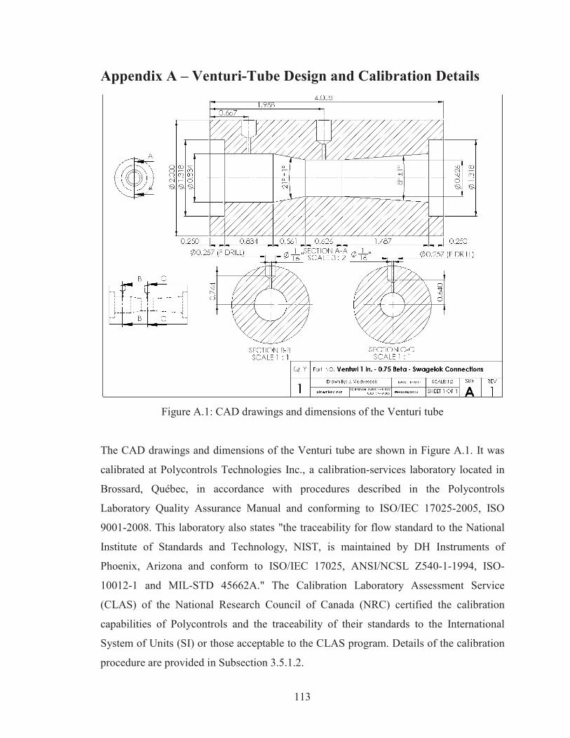
113
Appendix A – Venturi-Tube Design and Calibration Details
Figure A.1: CAD drawings and dimensions of the Venturi tube
The CAD drawings and dimensions of the Venturi tube are shown in Figure A.1. It was
calibrated at Polycontrols Technologies Inc., a calibration-services laboratory located in
Brossard, Québec, in accordance with procedures described in the Polycontrols
Laboratory Quality Assurance Manual and conforming to ISO/IEC 17025-2005, ISO
9001-2008. This laboratory also states "the traceability for flow standard to the National
Institute of Standards and Technology, NIST, is maintained by DH Instruments of
Phoenix, Arizona and conform to ISO/IEC 17025, ANSI/NCSL Z540-1-1994, ISO-
10012-1 and MIL-STD 45662A." The Calibration Laboratory Assessment Service
(CLAS) of the National Research Council of Canada (NRC) certified the calibration
capabilities of Polycontrols and the traceability of their standards to the International
System of Units (SI) or those acceptable to the CLAS program. Details of the calibration
procedure are provided in Subsection 3.5.1.2.
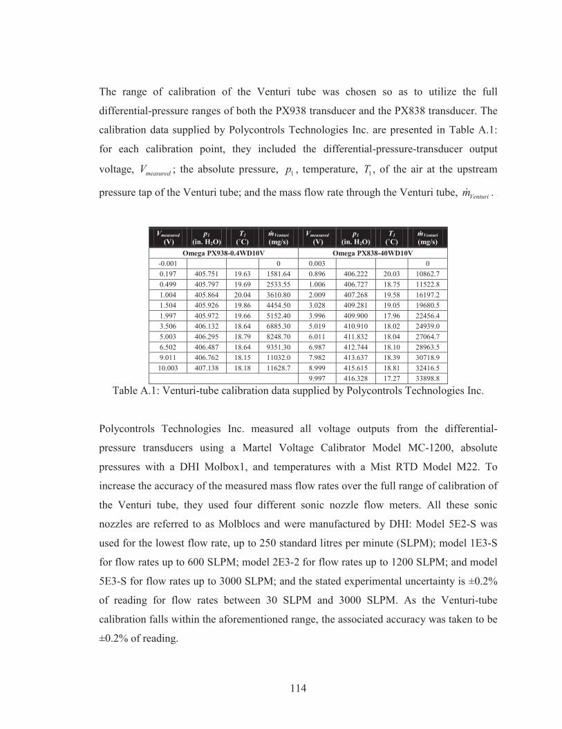
114
The range of calibration of the Venturi tube was chosen so as to utilize the full
differential-pressure ranges of both the PX938 transducer and the PX838 transducer. The
calibration data supplied by Polycontrols Technologies Inc. are presented in Table A.1:
for each calibration point, they included the differential-pressure-transducer output
voltage, measuredV ; the absolute pressure, 1p , temperature, 1T , of the air at the upstream
pressure tap of the Venturi tube; and the mass flow rate through the Venturi tube, Venturim .
Vmeasured
(V) p1
(in. H2O) T1
Venturi
(mg/s) Vmeasured
(V) p1
(in. H2O) T1
Venturi
(mg/s) Omega PX938-0.4WD10V Omega PX838-40WD10V
-0.001 0 0.003 0 0.197 405.751 19.63 1581.64 0.896 406.222 20.03 10862.7 0.499 405.797 19.69 2533.55 1.006 406.727 18.75 11522.8 1.004 405.864 20.04 3610.80 2.009 407.268 19.58 16197.2 1.504 405.926 19.86 4454.50 3.028 409.281 19.05 19680.5 1.997 405.972 19.66 5152.40 3.996 409.900 17.96 22456.4 3.506 406.132 18.64 6885.30 5.019 410.910 18.02 24939.0 5.003 406.295 18.79 8248.70 6.011 411.832 18.04 27064.7 6.502 406.487 18.64 9351.30 6.987 412.744 18.10 28963.5 9.011 406.762 18.15 11032.0 7.982 413.637 18.39 30718.9 10.003 407.138 18.18 11628.7 8.999 415.615 18.81 32416.5
9.997 416.328 17.27 33898.8
Table A.1: Venturi-tube calibration data supplied by Polycontrols Technologies Inc.
Polycontrols Technologies Inc. measured all voltage outputs from the differential-
pressure transducers using a Martel Voltage Calibrator Model MC-1200, absolute
pressures with a DHI Molbox1, and temperatures with a Mist RTD Model M22. To
increase the accuracy of the measured mass flow rates over the full range of calibration of
the Venturi tube, they used four different sonic nozzle flow meters. All these sonic
nozzles are referred to as Molblocs and were manufactured by DHI: Model 5E2-S was
used for the lowest flow rate, up to 250 standard litres per minute (SLPM); model 1E3-S
for flow rates up to 600 SLPM; model 2E3-2 for flow rates up to 1200 SLPM; and model
5E3-S for flow rates up to 3000 SLPM; and the stated experimental uncertainty is ±0.2%
of reading for flow rates between 30 SLPM and 3000 SLPM. As the Venturi-tube
calibration falls within the aforementioned range, the associated accuracy was taken to be
±0.2% of reading.
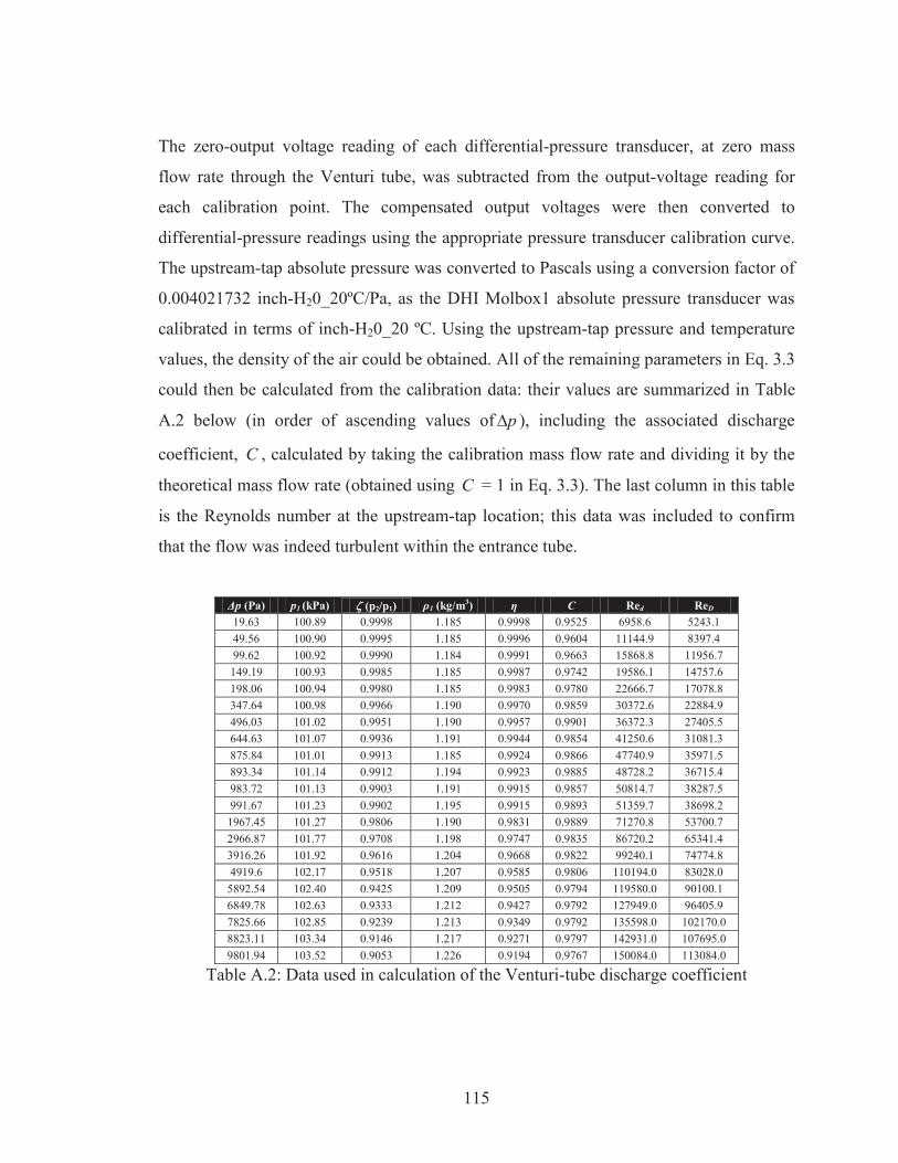
115
The zero-output voltage reading of each differential-pressure transducer, at zero mass
flow rate through the Venturi tube, was subtracted from the output-voltage reading for
each calibration point. The compensated output voltages were then converted to
differential-pressure readings using the appropriate pressure transducer calibration curve.
The upstream-tap absolute pressure was converted to Pascals using a conversion factor of
0.004021732 inch-H20_20ºC/Pa, as the DHI Molbox1 absolute pressure transducer was
calibrated in terms of inch-H20_20 ºC. Using the upstream-tap pressure and temperature
values, the density of the air could be obtained. All of the remaining parameters in Eq. 3.3
could then be calculated from the calibration data: their values are summarized in Table
A.2 below (in order of ascending values of p ), including the associated discharge
coefficient, C , calculated by taking the calibration mass flow rate and dividing it by the
theoretical mass flow rate (obtained using C = 1 in Eq. 3.3). The last column in this table
is the Reynolds number at the upstream-tap location; this data was included to confirm
that the flow was indeed turbulent within the entrance tube.
(Pa) p1 (kPa) (p2/p1) 1 (kg/m3) C Red ReD
19.63 100.89 0.9998 1.185 0.9998 0.9525 6958.6 5243.1 49.56 100.90 0.9995 1.185 0.9996 0.9604 11144.9 8397.4 99.62 100.92 0.9990 1.184 0.9991 0.9663 15868.8 11956.7 149.19 100.93 0.9985 1.185 0.9987 0.9742 19586.1 14757.6 198.06 100.94 0.9980 1.185 0.9983 0.9780 22666.7 17078.8 347.64 100.98 0.9966 1.190 0.9970 0.9859 30372.6 22884.9 496.03 101.02 0.9951 1.190 0.9957 0.9901 36372.3 27405.5 644.63 101.07 0.9936 1.191 0.9944 0.9854 41250.6 31081.3 875.84 101.01 0.9913 1.185 0.9924 0.9866 47740.9 35971.5 893.34 101.14 0.9912 1.194 0.9923 0.9885 48728.2 36715.4 983.72 101.13 0.9903 1.191 0.9915 0.9857 50814.7 38287.5 991.67 101.23 0.9902 1.195 0.9915 0.9893 51359.7 38698.2
1967.45 101.27 0.9806 1.190 0.9831 0.9889 71270.8 53700.7 2966.87 101.77 0.9708 1.198 0.9747 0.9835 86720.2 65341.4 3916.26 101.92 0.9616 1.204 0.9668 0.9822 99240.1 74774.8 4919.6 102.17 0.9518 1.207 0.9585 0.9806 110194.0 83028.0
5892.54 102.40 0.9425 1.209 0.9505 0.9794 119580.0 90100.1 6849.78 102.63 0.9333 1.212 0.9427 0.9792 127949.0 96405.9 7825.66 102.85 0.9239 1.213 0.9349 0.9792 135598.0 102170.0 8823.11 103.34 0.9146 1.217 0.9271 0.9797 142931.0 107695.0 9801.94 103.52 0.9053 1.226 0.9194 0.9767 150084.0 113084.0
Table A.2: Data used in calculation of the Venturi-tube discharge coefficient
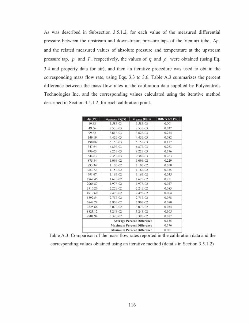
116
As was described in Subsection 3.5.1.2, for each value of the measured differential
pressure between the upstream and downstream pressure taps of the Venturi tube, p ,
and the related measured values of absolute pressure and temperature at the upstream
pressure tap, 1p and 1T , respectively, the values of and 1 were obtained (using Eq.
3.4 and property data for air); and then an iterative procedure was used to obtain the
corresponding mass flow rate, using Eqs. 3.3 to 3.6. Table A.3 summarizes the percent
difference between the mass flow rates in the calibration data supplied by Polycontrols
Technologies Inc. and the corresponding values calculated using the iterative method
described in Section 3.5.1.2, for each calibration point.
(Pa) calibration (kg/s) method (kg/s) Difference (%)
19.63 1.58E-03 1.58E-03 0.001 49.56 2.53E-03 2.53E-03 0.037 99.62 3.61E-03 3.62E-03 0.224
149.19 4.45E-03 4.45E-03 0.082 198.06 5.15E-03 5.15E-03 0.117 347.64 6.89E-03 6.87E-03 0.263 496.03 8.25E-03 8.22E-03 0.376 644.63 9.35E-03 9.38E-03 0.263 875.84 1.09E-02 1.09E-02 0.229 893.34 1.10E-02 1.10E-02 0.050 983.72 1.15E-02 1.16E-02 0.335 991.67 1.16E-02 1.16E-02 0.035
1967.45 1.62E-02 1.62E-02 0.251 2966.87 1.97E-02 1.97E-02 0.027 3916.26 2.25E-02 2.24E-02 0.083 4919.60 2.49E-02 2.49E-02 0.004 5892.54 2.71E-02 2.71E-02 0.078 6849.78 2.90E-02 2.90E-02 0.080 7825.66 3.07E-02 3.07E-02 0.034 8823.12 3.24E-02 3.24E-02 0.105 9801.94 3.39E-02 3.39E-02 0.017
Average Percent Difference 0.135 Maximum Percent Difference 0.376 Minimum Percent Difference 0.001
Table A.3: Comparison of the mass flow rates reported in the calibration data and the
corresponding values obtained using an iterative method (details in Section 3.5.1.2)
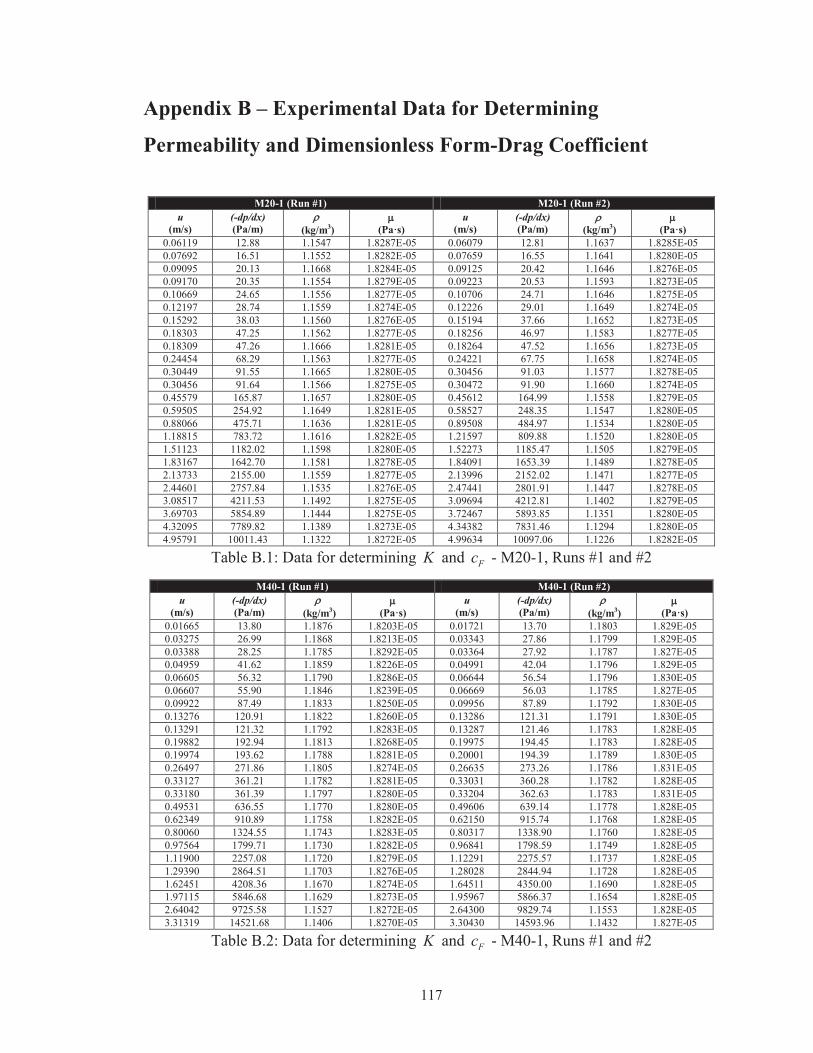
117
Appendix B – Experimental Data for Determining
Permeability and Dimensionless Form-Drag Coefficient
M20-1 (Run #1) M20-1 (Run #2) u
(m/s) (-dp/dx) (Pa/m) (kg/m3)
(Pa·s)
u (m/s)
(-dp/dx) (Pa/m) (kg/m3) (Pa·s)
0.06119 12.88 1.1547 1.8287E-05 0.06079 12.81 1.1637 1.8285E-05 0.07692 16.51 1.1552 1.8282E-05 0.07659 16.55 1.1641 1.8280E-05 0.09095 20.13 1.1668 1.8284E-05 0.09125 20.42 1.1646 1.8276E-05 0.09170 20.35 1.1554 1.8279E-05 0.09223 20.53 1.1593 1.8273E-05 0.10669 24.65 1.1556 1.8277E-05 0.10706 24.71 1.1646 1.8275E-05 0.12197 28.74 1.1559 1.8274E-05 0.12226 29.01 1.1649 1.8274E-05 0.15292 38.03 1.1560 1.8276E-05 0.15194 37.66 1.1652 1.8273E-05 0.18303 47.25 1.1562 1.8277E-05 0.18256 46.97 1.1583 1.8277E-05 0.18309 47.26 1.1666 1.8281E-05 0.18264 47.52 1.1656 1.8273E-05 0.24454 68.29 1.1563 1.8277E-05 0.24221 67.75 1.1658 1.8274E-05 0.30449 91.55 1.1665 1.8280E-05 0.30456 91.03 1.1577 1.8278E-05 0.30456 91.64 1.1566 1.8275E-05 0.30472 91.90 1.1660 1.8274E-05 0.45579 165.87 1.1657 1.8280E-05 0.45612 164.99 1.1558 1.8279E-05 0.59505 254.92 1.1649 1.8281E-05 0.58527 248.35 1.1547 1.8280E-05 0.88066 475.71 1.1636 1.8281E-05 0.89508 484.97 1.1534 1.8280E-05 1.18815 783.72 1.1616 1.8282E-05 1.21597 809.88 1.1520 1.8280E-05 1.51123 1182.02 1.1598 1.8280E-05 1.52273 1185.47 1.1505 1.8279E-05 1.83167 1642.70 1.1581 1.8278E-05 1.84091 1653.39 1.1489 1.8278E-05 2.13733 2155.00 1.1559 1.8277E-05 2.13996 2152.02 1.1471 1.8277E-05 2.44601 2757.84 1.1535 1.8276E-05 2.47441 2801.91 1.1447 1.8278E-05 3.08517 4211.53 1.1492 1.8275E-05 3.09694 4212.81 1.1402 1.8279E-05 3.69703 5854.89 1.1444 1.8275E-05 3.72467 5893.85 1.1351 1.8280E-05 4.32095 7789.82 1.1389 1.8273E-05 4.34382 7831.46 1.1294 1.8280E-05 4.95791 10011.43 1.1322 1.8272E-05 4.99634 10097.06 1.1226 1.8282E-05
Table B.1: Data for determining K and Fc - M20-1, Runs #1 and #2
M40-1 (Run #1) M40-1 (Run #2) u
(m/s) (-dp/dx) (Pa/m) (kg/m3)
(Pa·s)
u (m/s)
(-dp/dx) (Pa/m) (kg/m3)
(Pa·s)
0.01665 13.80 1.1876 1.8203E-05 0.01721 13.70 1.1803 1.829E-05 0.03275 26.99 1.1868 1.8213E-05 0.03343 27.86 1.1799 1.829E-05 0.03388 28.25 1.1785 1.8292E-05 0.03364 27.92 1.1787 1.827E-05 0.04959 41.62 1.1859 1.8226E-05 0.04991 42.04 1.1796 1.829E-05 0.06605 56.32 1.1790 1.8286E-05 0.06644 56.54 1.1796 1.830E-05 0.06607 55.90 1.1846 1.8239E-05 0.06669 56.03 1.1785 1.827E-05 0.09922 87.49 1.1833 1.8250E-05 0.09956 87.89 1.1792 1.830E-05 0.13276 120.91 1.1822 1.8260E-05 0.13286 121.31 1.1791 1.830E-05 0.13291 121.32 1.1792 1.8283E-05 0.13287 121.46 1.1783 1.828E-05 0.19882 192.94 1.1813 1.8268E-05 0.19975 194.45 1.1783 1.828E-05 0.19974 193.62 1.1788 1.8281E-05 0.20001 194.39 1.1789 1.830E-05 0.26497 271.86 1.1805 1.8274E-05 0.26635 273.26 1.1786 1.831E-05 0.33127 361.21 1.1782 1.8281E-05 0.33031 360.28 1.1782 1.828E-05 0.33180 361.39 1.1797 1.8280E-05 0.33204 362.63 1.1783 1.831E-05 0.49531 636.55 1.1770 1.8280E-05 0.49606 639.14 1.1778 1.828E-05 0.62349 910.89 1.1758 1.8282E-05 0.62150 915.74 1.1768 1.828E-05 0.80060 1324.55 1.1743 1.8283E-05 0.80317 1338.90 1.1760 1.828E-05 0.97564 1799.71 1.1730 1.8282E-05 0.96841 1798.59 1.1749 1.828E-05 1.11900 2257.08 1.1720 1.8279E-05 1.12291 2275.57 1.1737 1.828E-05 1.29390 2864.51 1.1703 1.8276E-05 1.28028 2844.94 1.1728 1.828E-05 1.62451 4208.36 1.1670 1.8274E-05 1.64511 4350.00 1.1690 1.828E-05 1.97115 5846.68 1.1629 1.8273E-05 1.95967 5866.37 1.1654 1.828E-05 2.64042 9725.58 1.1527 1.8272E-05 2.64300 9829.74 1.1553 1.828E-05 3.31319 14521.68 1.1406 1.8270E-05 3.30430 14593.96 1.1432 1.827E-05
Table B.2: Data for determining K and Fc - M40-1, Runs #1 and #2
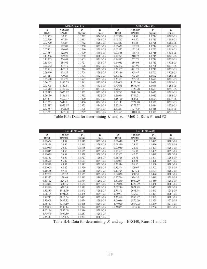
118
M60-2 (Run #1) M60-2 (Run #2) u
(m/s) (-dp/dx) (Pa/m) (kg/m3)
(Pa·s)
u (m/s)
(-dp/dx) (Pa/m) (kg/m3)
(Pa·s)
0.01853 33.75 1.1772 1.826E-05 0.01926 34.89 1.1714 1.829E-05 0.03769 60.20 1.1615 1.829E-05 0.03767 68.27 1.1713 1.829E-05 0.03770 68.19 1.1762 1.826E-05 0.03843 61.16 1.1728 1.826E-05 0.05641 102.07 1.1750 1.827E-05 0.05632 102.20 1.1714 1.829E-05 0.07471 136.65 1.1740 1.828E-05 0.07522 122.35 1.1723 1.826E-05 0.07557 122.91 1.1609 1.830E-05 0.07548 138.43 1.1715 1.830E-05 0.11236 209.27 1.1730 1.828E-05 0.11291 210.72 1.1715 1.830E-05 0.15003 254.49 1.1605 1.831E-05 0.14897 252.71 1.1716 1.827E-05 0.15004 284.62 1.1721 1.828E-05 0.14985 284.96 1.1713 1.830E-05 0.22562 397.19 1.1598 1.832E-05 0.22462 394.95 1.1706 1.827E-05 0.22585 442.11 1.1714 1.829E-05 0.22567 441.25 1.1712 1.830E-05 0.29990 603.27 1.1704 1.829E-05 0.30186 608.47 1.1705 1.830E-05 0.37611 709.26 1.1591 1.832E-05 0.37312 703.29 1.1692 1.828E-05 0.37620 785.70 1.1697 1.829E-05 0.37553 785.37 1.1697 1.830E-05 0.56152 1182.73 1.1581 1.832E-05 0.56008 1176.66 1.1678 1.828E-05 0.73775 1742.61 1.1567 1.833E-05 0.70675 1636.46 1.1669 1.828E-05 0.92512 2377.26 1.1551 1.833E-05 0.90667 2320.78 1.1653 1.828E-05 1.09013 3025.12 1.1532 1.833E-05 1.09283 3049.00 1.1632 1.828E-05 1.29130 3866.18 1.1512 1.833E-05 1.26964 3789.21 1.1613 1.828E-05 1.47231 4697.37 1.1490 1.833E-05 1.45120 4604.11 1.1594 1.827E-05 1.85765 6642.01 1.1436 1.834E-05 1.87143 6724.70 1.1539 1.827E-05 2.25817 8953.07 1.1373 1.834E-05 2.22294 8773.77 1.1484 1.827E-05 2.63757 11421.66 1.1305 1.834E-05 2.61217 11277.44 1.1418 1.827E-05 3.03741 14270.14 1.1229 1.834E-05 3.01575 14183.71 1.1339 1.827E-05
Table B.3: Data for determining K and Fc - M60-2, Runs #1 and #2
ERG40 (Run #1) ERG40 (Run #2)
u (m/s)
(-dp/dx) (Pa/m) (kg/m3)
(Pa·s)
u (m/s)
(-dp/dx) (Pa/m) (kg/m3)
(Pa·s)
0.06654 19.54 1.1549 1.829E-05 0.06640 19.25 1.1499 1.828E-05 0.08358 24.90 1.1543 1.829E-05 0.08350 25.00 1.1496 1.828E-05 0.09969 30.47 1.1536 1.829E-05 0.09950 30.30 1.1491 1.828E-05 0.10045 30.53 1.1535 1.829E-05 0.11587 36.06 1.1489 1.829E-05 0.11656 36.68 1.1539 1.829E-05 0.13303 42.25 1.1488 1.829E-05 0.13381 42.69 1.1527 1.829E-05 0.16526 54.73 1.1491 1.829E-05 0.16650 55.47 1.1523 1.829E-05 0.20021 68.21 1.1498 1.829E-05 0.19970 68.52 1.1545 1.829E-05 0.26544 96.65 1.1500 1.828E-05 0.20000 68.42 1.1520 1.829E-05 0.33394 129.67 1.1502 1.828E-05 0.26665 97.33 1.1515 1.829E-05 0.49724 227.32 1.1501 1.828E-05 0.33269 129.32 1.1535 1.829E-05 0.64038 338.51 1.1496 1.828E-05 0.33322 129.66 1.1513 1.830E-05 0.97714 634.32 1.1488 1.828E-05 0.49112 224.34 1.1534 1.829E-05 1.31239 1007.29 1.1480 1.828E-05 0.62814 328.36 1.1524 1.829E-05 1.65036 1470.29 1.1468 1.828E-05 0.96816 628.38 1.1511 1.829E-05 2.00246 2021.48 1.1455 1.828E-05 1.31350 1011.79 1.1495 1.829E-05 2.34195 2635.94 1.1443 1.828E-05 1.66304 1491.25 1.1485 1.829E-05 2.68963 3363.91 1.1424 1.828E-05 1.99743 2013.34 1.1475 1.829E-05 3.36588 4953.97 1.1382 1.828E-05 2.33908 2635.33 1.1454 1.829E-05 4.06086 6870.09 1.1328 1.827E-05 2.68733 3356.19 1.1438 1.829E-05 4.74020 9034.72 1.1269 1.827E-05 3.38062 4988.14 1.1394 1.829E-05 5.36825 11235.94 1.1206 1.827E-05 4.05194 6855.09 1.1344 1.829E-05 4.71699 9007.80 1.1287 1.828E-05 5.35441 11254.77 1.1227 1.828E-05
Table B.4: Data for determining K and Fc - ERG40, Runs #1 and #2
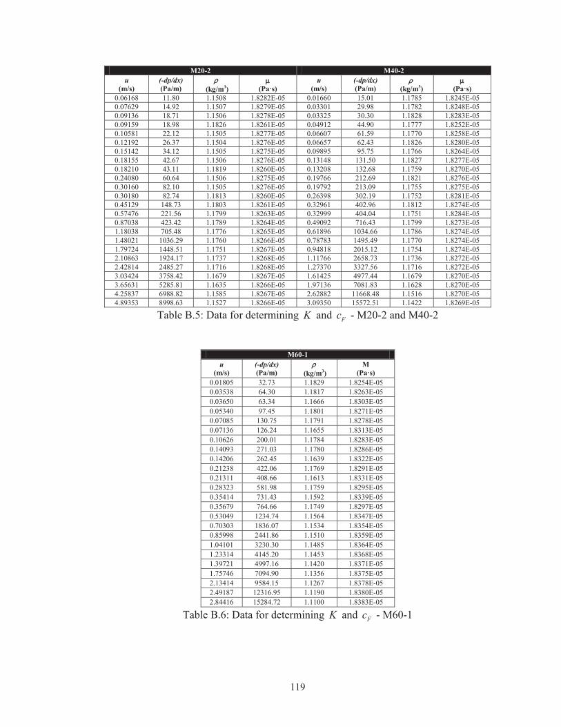
119
M20-2 M40-2 u
(m/s) (-dp/dx) (Pa/m) (kg/m3)
(Pa·s)
u (m/s)
(-dp/dx) (Pa/m) (kg/m3) (Pa·s)
0.06168 11.80 1.1508 1.8282E-05 0.01660 15.01 1.1785 1.8245E-05 0.07629 14.92 1.1507 1.8279E-05 0.03301 29.98 1.1782 1.8248E-05 0.09136 18.71 1.1506 1.8278E-05 0.03325 30.30 1.1828 1.8283E-05 0.09159 18.98 1.1826 1.8261E-05 0.04912 44.90 1.1777 1.8252E-05 0.10581 22.12 1.1505 1.8277E-05 0.06607 61.59 1.1770 1.8258E-05 0.12192 26.37 1.1504 1.8276E-05 0.06657 62.43 1.1826 1.8280E-05 0.15142 34.12 1.1505 1.8275E-05 0.09895 95.75 1.1766 1.8264E-05 0.18155 42.67 1.1506 1.8276E-05 0.13148 131.50 1.1827 1.8277E-05 0.18210 43.11 1.1819 1.8260E-05 0.13208 132.68 1.1759 1.8270E-05 0.24080 60.64 1.1506 1.8275E-05 0.19766 212.69 1.1821 1.8276E-05 0.30160 82.10 1.1505 1.8276E-05 0.19792 213.09 1.1755 1.8275E-05 0.30180 82.74 1.1813 1.8260E-05 0.26398 302.19 1.1752 1.8281E-05 0.45129 148.73 1.1803 1.8261E-05 0.32961 402.96 1.1812 1.8274E-05 0.57476 221.56 1.1799 1.8263E-05 0.32999 404.04 1.1751 1.8284E-05 0.87038 423.42 1.1789 1.8264E-05 0.49092 716.43 1.1799 1.8273E-05 1.18038 705.48 1.1776 1.8265E-05 0.61896 1034.66 1.1786 1.8274E-05 1.48021 1036.29 1.1760 1.8266E-05 0.78783 1495.49 1.1770 1.8274E-05 1.79724 1448.51 1.1751 1.8267E-05 0.94818 2015.12 1.1754 1.8274E-05 2.10863 1924.17 1.1737 1.8268E-05 1.11766 2658.73 1.1736 1.8272E-05 2.42814 2485.27 1.1716 1.8268E-05 1.27370 3327.56 1.1716 1.8272E-05 3.03424 3758.42 1.1679 1.8267E-05 1.61425 4977.44 1.1679 1.8270E-05 3.65631 5285.81 1.1635 1.8266E-05 1.97136 7081.83 1.1628 1.8270E-05 4.25837 6988.82 1.1585 1.8267E-05 2.62882 11668.48 1.1516 1.8270E-05 4.89353 8998.63 1.1527 1.8266E-05 3.09350 15572.51 1.1422 1.8269E-05
Table B.5: Data for determining K and Fc - M20-2 and M40-2
M60-1
u (m/s)
(-dp/dx) (Pa/m) (kg/m3)
M (Pa·s)
0.01805 32.73 1.1829 1.8254E-05 0.03538 64.30 1.1817 1.8263E-05 0.03650 63.34 1.1666 1.8303E-05 0.05340 97.45 1.1801 1.8271E-05 0.07085 130.75 1.1791 1.8278E-05 0.07136 126.24 1.1655 1.8313E-05 0.10626 200.01 1.1784 1.8283E-05 0.14093 271.03 1.1780 1.8286E-05 0.14206 262.45 1.1639 1.8322E-05 0.21238 422.06 1.1769 1.8291E-05 0.21311 408.66 1.1613 1.8331E-05 0.28323 581.98 1.1759 1.8295E-05 0.35414 731.43 1.1592 1.8339E-05 0.35679 764.66 1.1749 1.8297E-05 0.53049 1234.74 1.1564 1.8347E-05 0.70303 1836.07 1.1534 1.8354E-05 0.85998 2441.86 1.1510 1.8359E-05 1.04101 3230.30 1.1485 1.8364E-05 1.23314 4145.20 1.1453 1.8368E-05 1.39721 4997.16 1.1420 1.8371E-05 1.75746 7094.90 1.1356 1.8375E-05 2.13414 9584.15 1.1267 1.8378E-05 2.49187 12316.95 1.1190 1.8380E-05 2.84416 15284.72 1.1100 1.8383E-05
Table B.6: Data for determining K and Fc - M60-1
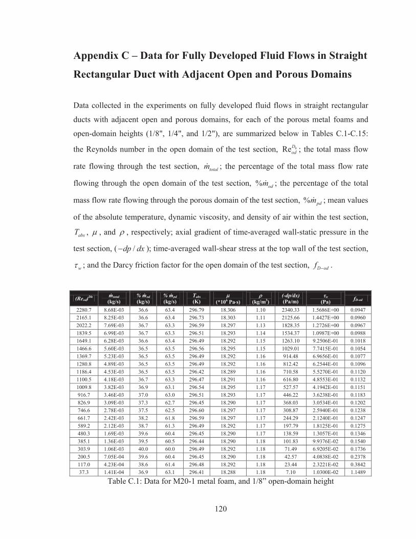
120
Appendix C – Data for Fully Developed Fluid Flows in Straight
Rectangular Duct with Adjacent Open and Porous Domains
Data collected in the experiments on fully developed fluid flows in straight rectangular
ducts with adjacent open and porous domains, for each of the porous metal foams and
open-domain heights (1/8", 1/4", and 1/2"), are summarized below in Tables C.1-C.15:
the Reynolds number in the open domain of the test section, Re hDod ; the total mass flow
rate flowing through the test section, totalm ; the percentage of the total mass flow rate
flowing through the open domain of the test section, % odm ; the percentage of the total
mass flow rate flowing through the porous domain of the test section, % pdm ; mean values
of the absolute temperature, dynamic viscosity, and density of air within the test section,
absT , , and , respectively; axial gradient of time-averaged wall-static pressure in the
test section, ( /dp dx ); time-averaged wall-shear stress at the top wall of the test section,
w ; and the Darcy friction factor for the open domain of the test section, D odf .
(Reod)Dh total (kg/s)
% od (kg/s)
% pd (kg/s)
Tabs (K)
(*106 Pa s)
(kg/m3)
(-dp/dx) (Pa/m)
w (Pa)
fD-od
2280.7 8.68E-03 36.6 63.4 296.79 18.306 1.10 2340.33 1.5686E+00 0.0947 2165.1 8.25E-03 36.6 63.4 296.73 18.303 1.11 2125.66 1.4427E+00 0.0960 2022.2 7.69E-03 36.7 63.3 296.59 18.297 1.13 1828.35 1.2726E+00 0.0967 1839.5 6.99E-03 36.7 63.3 296.51 18.293 1.14 1534.37 1.0987E+00 0.0988 1649.1 6.28E-03 36.6 63.4 296.49 18.292 1.15 1263.10 9.2506E-01 0.1018 1466.6 5.60E-03 36.5 63.5 296.56 18.295 1.15 1029.01 7.7415E-01 0.1054 1369.7 5.23E-03 36.5 63.5 296.49 18.292 1.16 914.48 6.9656E-01 0.1077 1280.8 4.89E-03 36.5 63.5 296.49 18.292 1.16 812.42 6.2544E-01 0.1096 1186.4 4.53E-03 36.5 63.5 296.42 18.289 1.16 710.58 5.5270E-01 0.1120 1100.5 4.18E-03 36.7 63.3 296.47 18.291 1.16 616.80 4.8553E-01 0.1132 1009.8 3.82E-03 36.9 63.1 296.54 18.295 1.17 527.57 4.1942E-01 0.1151 916.7 3.46E-03 37.0 63.0 296.51 18.293 1.17 446.22 3.6238E-01 0.1183 826.9 3.09E-03 37.3 62.7 296.45 18.290 1.17 368.03 3.0534E-01 0.1202 746.6 2.78E-03 37.5 62.5 296.60 18.297 1.17 308.87 2.5940E-01 0.1238 661.7 2.42E-03 38.2 61.8 296.59 18.297 1.17 244.29 2.1240E-01 0.1247 589.2 2.12E-03 38.7 61.3 296.49 18.292 1.17 197.79 1.8125E-01 0.1275 480.3 1.69E-03 39.6 60.4 296.45 18.290 1.17 138.59 1.3057E-01 0.1346 385.1 1.36E-03 39.5 60.5 296.44 18.290 1.18 101.83 9.9376E-02 0.1540 303.9 1.06E-03 40.0 60.0 296.49 18.292 1.18 71.49 6.9205E-02 0.1736 200.5 7.05E-04 39.6 60.4 296.45 18.290 1.18 42.57 4.0838E-02 0.2378 117.0 4.23E-04 38.6 61.4 296.48 18.292 1.18 23.44 2.3221E-02 0.3842 37.3 1.41E-04 36.9 63.1 296.41 18.288 1.18 7.10 1.0300E-02 1.1489
Table C.1: Data for M20-1 metal foam, and 1/8” open-domain height

121
(Reod)Dh total (kg/s)
% od (kg/s)
% pd (kg/s)
Tabs (K)
(*106 Pa s)
(kg/m3)
(-dp/dx) (Pa/m)
w (Pa)
fD-od
8392.8 1.55E-02 75.7 24.3 296.65 18.300 1.14 1152.33 1.5742E+00 0.0957 7779.4 1.43E-02 75.9 24.1 296.67 18.301 1.14 982.24 1.3629E+00 0.0954 7056.4 1.29E-02 76.1 23.9 296.69 18.302 1.15 813.96 1.1370E+00 0.0966 6315.5 1.15E-02 76.3 23.7 296.68 18.301 1.15 655.68 9.2762E-01 0.0977 5582.9 1.02E-02 76.6 23.4 296.64 18.299 1.16 517.72 7.3912E-01 0.0991 4801.8 8.71E-03 76.9 23.1 296.70 18.302 1.16 394.61 5.6155E-01 0.1025 4413.3 7.99E-03 77.0 23.0 296.74 18.304 1.17 339.16 4.8144E-01 0.1044 4008.7 7.24E-03 77.2 22.8 296.69 18.302 1.17 287.27 4.0757E-01 0.1074 3620.9 6.52E-03 77.4 22.6 296.69 18.302 1.17 240.02 3.4164E-01 0.1101 3219.2 5.78E-03 77.7 22.3 296.67 18.301 1.17 195.01 2.7985E-01 0.1135 3022.2 5.41E-03 77.9 22.1 296.68 18.301 1.17 174.92 2.5053E-01 0.1155 2816.4 5.03E-03 78.1 21.9 296.72 18.303 1.17 154.94 2.2254E-01 0.1179 2616.0 4.66E-03 78.3 21.7 296.71 18.303 1.17 136.06 1.9979E-01 0.1200 2418.7 4.29E-03 78.6 21.4 296.69 18.302 1.17 118.45 1.7636E-01 0.1223 2226.2 3.93E-03 79.1 20.9 296.68 18.301 1.17 101.54 1.5306E-01 0.1238 2010.3 3.53E-03 79.4 20.6 296.74 18.304 1.17 85.77 1.2998E-01 0.1282 1828.3 3.19E-03 80.0 20.0 296.71 18.303 1.18 71.61 1.1064E-01 0.1295 1625.8 2.81E-03 80.7 19.3 296.68 18.301 1.18 57.87 9.1148E-02 0.1324 1433.4 2.45E-03 81.6 18.4 296.65 18.300 1.18 45.90 7.3506E-02 0.1351 1241.5 2.10E-03 82.5 17.5 296.75 18.304 1.18 35.60 5.7987E-02 0.1396 1030.2 1.72E-03 83.3 16.7 296.60 18.297 1.18 26.49 4.3403E-02 0.1510 876.1 1.45E-03 84.3 15.7 296.68 18.301 1.18 20.12 3.3518E-02 0.1585 664.8 1.08E-03 85.8 14.2 296.71 18.302 1.18 12.91 2.2048E-02 0.1766 461.7 7.20E-04 89.4 10.6 296.72 18.303 1.18 6.05 1.4883E-02 0.1715
Table C.2: Data for M20-1 metal foam, and 1/4” open-domain height
(Reod)Dh total (kg/s)
% od (kg/s)
% pd (kg/s)
Tabs (K)
(*106 Pa s)
(kg/m3)
(-dp/dx) (Pa/m)
w (Pa)
fD-od
13664.0 2.05E-02 93.3 6.7 297.35 18.333 1.16 214.68 6.7856E-01 0.0891 12886.3 1.93E-02 93.4 6.6 297.35 18.333 1.16 191.21 6.0135E-01 0.0893 11971.6 1.79E-02 93.6 6.4 297.33 18.332 1.16 164.25 5.2000E-01 0.0891 11015.5 1.64E-02 93.8 6.2 297.34 18.333 1.17 136.87 4.3677E-01 0.0878 10109.2 1.50E-02 94.0 6.0 297.34 18.333 1.17 115.16 3.6563E-01 0.0879 9155.0 1.36E-02 94.3 5.7 297.35 18.333 1.17 94.89 2.9928E-01 0.0884 8198.2 1.21E-02 94.5 5.5 297.35 18.333 1.17 76.99 2.4428E-01 0.0896 7187.2 1.06E-02 94.7 5.3 297.35 18.333 1.17 60.38 1.9465E-01 0.0915 6212.8 9.13E-03 95.1 4.9 297.33 18.332 1.17 45.89 1.5120E-01 0.0932 5164.7 7.56E-03 95.4 4.6 297.33 18.332 1.18 32.93 1.1124E-01 0.0968 4635.4 6.77E-03 95.6 4.4 297.34 18.333 1.18 27.25 9.3299E-02 0.0995 4122.5 6.01E-03 95.9 4.1 297.35 18.333 1.18 22.05 7.6692E-02 0.1018 3884.5 5.65E-03 96.1 3.9 297.36 18.334 1.18 19.57 6.9835E-02 0.1018 3619.8 5.25E-03 96.2 3.8 297.38 18.335 1.18 17.11 6.2162E-02 0.1025 3338.2 4.84E-03 96.4 3.6 297.40 18.336 1.18 14.67 5.4692E-02 0.1033 3108.4 4.49E-03 96.7 3.3 297.41 18.336 1.18 12.47 4.9645E-02 0.1013 2828.9 4.08E-03 96.8 3.2 297.24 18.328 1.18 10.75 4.4850E-02 0.1056 2569.7 3.71E-03 96.9 3.1 297.32 18.332 1.18 9.47 3.9681E-02 0.1126 2318.3 3.34E-03 97.1 2.9 297.39 18.335 1.18 7.82 3.5464E-02 0.1142 2048.7 2.93E-03 97.5 2.5 297.24 18.328 1.18 5.77 3.0702E-02 0.1080 1811.9 2.58E-03 98.1 1.9 297.31 18.331 1.18 3.74 2.6182E-02 0.0895
Table C.3: Data for M20-1 metal foam, and 1/2” open-domain height

122
(Reod)Dh total (kg/s)
% od (kg/s)
% pd (kg/s)
Tabs (K)
(*106 Pa s)
(kg/m3)
(-dp/dx) (Pa/m)
w (Pa)
fD-od
4692.2 8.92E-03 73.4 26.6 296.93 18.313 1.09 2072.44 1.9199E+00 0.1047 4351.9 8.26E-03 73.5 26.5 296.94 18.314 1.09 1827.48 1.6933E+00 0.1074 4027.4 7.62E-03 73.8 26.2 296.96 18.315 1.10 1570.46 1.4810E+00 0.1086 3680.1 6.94E-03 74.0 26.0 296.98 18.316 1.11 1329.53 1.2807E+00 0.1109 3324.2 6.24E-03 74.3 25.7 296.95 18.314 1.11 1106.43 1.0887E+00 0.1139 2965.9 5.54E-03 74.7 25.3 296.98 18.315 1.12 900.09 8.9062E-01 0.1171 2792.3 5.20E-03 74.9 25.1 297.00 18.316 1.12 808.63 7.9980E-01 0.1190 2611.3 4.85E-03 75.2 24.8 296.96 18.314 1.13 714.75 7.1609E-01 0.1208 2431.0 4.49E-03 75.5 24.5 296.96 18.315 1.13 627.91 6.3131E-01 0.1227 2253.6 4.14E-03 75.9 24.1 296.96 18.315 1.13 548.22 5.5408E-01 0.1250 2077.0 3.80E-03 76.3 23.7 296.97 18.315 1.14 474.95 4.7854E-01 0.1277 1898.7 3.45E-03 76.8 23.2 296.93 18.313 1.14 404.22 4.0600E-01 0.1304 1721.5 3.10E-03 77.5 22.5 296.95 18.314 1.14 337.03 3.4118E-01 0.1325 1537.1 2.75E-03 78.1 21.9 296.96 18.315 1.14 276.52 2.8104E-01 0.1366 1375.4 2.43E-03 79.0 21.0 296.95 18.314 1.14 225.09 2.3317E-01 0.1392 1187.6 2.07E-03 80.2 19.8 296.92 18.313 1.15 171.42 1.8602E-01 0.1424 1003.6 1.72E-03 81.6 18.4 296.93 18.313 1.15 125.65 1.3952E-01 0.1464 828.8 1.39E-03 83.2 16.8 296.95 18.314 1.15 88.45 1.0117E-01 0.1513 639.7 1.04E-03 85.6 14.4 296.94 18.314 1.15 54.58 6.5036E-02 0.1569 439.7 6.98E-04 87.8 12.2 296.93 18.313 1.15 29.57 3.7143E-02 0.1801 265.7 4.20E-04 88.3 11.7 296.95 18.314 1.15 16.73 2.1855E-02 0.2792 88.2 1.40E-04 88.1 11.9 296.93 18.313 1.15 5.57 8.4152E-03 0.8441
Table C.4: Data for M40-1 metal foam, and 1/8” open-domain height
(Reod)Dh total (kg/s)
% od (kg/s)
% pd (kg/s)
Tabs (K)
(*106 Pa s)
(kg/m3)
(-dp/dx) (Pa/m)
w (Pa)
fD-od
10207.7 1.57E-02 90.8 9.2 296.63 18.299 1.14 920.72 1.5296E+00 0.1014 9419.6 1.44E-02 91.1 8.9 296.63 18.299 1.15 770.27 1.3023E+00 0.1002 8542.3 1.30E-02 91.4 8.6 296.64 18.299 1.15 628.12 1.0798E+00 0.0999 7652.8 1.16E-02 91.8 8.2 296.61 18.298 1.16 503.36 8.7177E-01 0.1003 6771.0 1.02E-02 92.2 7.8 296.59 18.297 1.16 392.97 6.8451E-01 0.1004 5835.0 8.78E-03 92.6 7.4 296.53 18.294 1.17 296.83 5.1769E-01 0.1026 5373.2 8.06E-03 92.9 7.1 296.64 18.299 1.17 253.46 4.4507E-01 0.1034 4871.0 7.28E-03 93.2 6.8 296.36 18.286 1.17 211.51 3.7203E-01 0.1053 4415.6 6.59E-03 93.5 6.5 296.60 18.297 1.17 176.95 3.0831E-01 0.1071 3948.4 5.87E-03 93.8 6.2 296.78 18.306 1.17 144.36 2.5102E-01 0.1093 3659.1 5.42E-03 94.1 5.9 296.64 18.299 1.17 125.51 2.2169E-01 0.1108 3433.8 5.08E-03 94.3 5.7 296.63 18.299 1.18 111.89 2.0002E-01 0.1122 3193.2 4.71E-03 94.5 5.5 296.55 18.295 1.18 97.48 1.7825E-01 0.1131 2938.5 4.33E-03 94.7 5.3 296.64 18.299 1.18 84.31 1.5385E-01 0.1154 2684.1 3.95E-03 94.9 5.1 296.65 18.300 1.18 74.05 1.3358E-01 0.1215 2487.1 3.64E-03 95.1 4.9 296.46 18.291 1.18 63.96 1.1761E-01 0.1224 2187.6 3.19E-03 95.5 4.5 296.38 18.287 1.18 51.14 9.4901E-02 0.1266 1951.6 2.84E-03 95.8 4.2 296.47 18.291 1.18 41.99 7.7447E-02 0.1305 1717.3 2.49E-03 96.2 3.8 296.56 18.295 1.18 32.53 6.2177E-02 0.1306 1462.8 2.11E-03 96.7 3.3 296.45 18.290 1.18 23.66 4.8050E-02 0.1310 1220.7 1.75E-03 97.4 2.6 296.57 18.296 1.18 15.09 3.5283E-02 0.1198 1010.6 1.44E-03 98.0 2.0 296.71 18.303 1.18 9.39 2.8511E-02 0.1086 772.3 1.09E-03 98.5 1.5 296.69 18.302 1.17 5.44 1.7639E-02 0.1077 515.6 7.30E-04 98.5 1.5 296.41 18.288 1.18 3.63 1.3697E-02 0.1617
Table C.5: Data for M40-1 metal foam, and 1/4” open-domain height

123
(Reod)Dh total (kg/s)
% od (kg/s)
% pd (kg/s)
Tabs (K)
(*106 Pa s)
(kg/m3)
(-dp/dx) (Pa/m)
w (Pa)
fD-od
14346.0 2.09E-02 95.5 4.5 295.73 18.256 1.18 175.37 5.8848E-01 0.0927 13386.5 1.95E-02 95.7 4.3 295.70 18.254 1.18 152.08 5.1276E-01 0.0925 12367.9 1.79E-02 95.9 4.1 295.69 18.254 1.18 129.02 4.3689E-01 0.0921 11496.2 1.66E-02 96.1 3.9 295.70 18.254 1.19 109.64 3.7009E-01 0.0908 10526.2 1.52E-02 96.3 3.7 295.69 18.253 1.19 91.50 3.1190E-01 0.0905 9528.5 1.37E-02 96.5 3.5 295.66 18.252 1.19 74.69 2.5321E-01 0.0903 8533.6 1.23E-02 96.7 3.3 295.89 18.263 1.19 60.19 2.0373E-01 0.0907 7538.9 1.08E-02 97.0 3.0 295.96 18.267 1.19 46.90 1.6355E-01 0.0906 6497.7 9.30E-03 97.3 2.7 295.89 18.263 1.19 35.16 1.2697E-01 0.0916 5381.4 7.67E-03 97.6 2.4 295.80 18.259 1.20 24.77 9.2514E-02 0.0942 4839.4 6.88E-03 97.8 2.2 295.72 18.255 1.20 20.04 7.7854E-02 0.0944 4355.3 6.18E-03 98.0 2.0 295.68 18.253 1.20 16.13 6.6434E-02 0.0939 4019.0 5.69E-03 98.1 1.9 295.54 18.246 1.20 13.63 5.8264E-02 0.0933 3752.3 5.31E-03 98.3 1.7 295.81 18.259 1.20 11.83 5.0635E-02 0.0927 3529.5 4.99E-03 98.4 1.6 295.86 18.262 1.20 10.12 4.5354E-02 0.0896 3200.0 4.51E-03 98.7 1.3 295.73 18.256 1.20 7.59 3.9308E-02 0.0819 3020.2 4.25E-03 98.8 1.2 295.91 18.264 1.20 6.13 3.6985E-02 0.0741 2680.7 3.76E-03 99.2 0.8 295.81 18.259 1.20 3.62 3.6130E-02 0.0556 2483.8 3.47E-03 99.5 0.5 295.66 18.252 1.20 2.31 3.3363E-02 0.0414 2242.4 3.14E-03 99.5 0.5 295.81 18.259 1.20 2.02 2.7586E-02 0.0443 1865.2 2.61E-03 99.6 0.4 295.75 18.257 1.20 1.32 2.1326E-02 0.0419
Table C.6: Data for M40-1 metal foam, and 1/2” open-domain height
(Reod)Dh total (kg/s)
% od (kg/s)
% pd (kg/s)
Tabs (K)
(*106 Pa s)
(kg/m3)
(-dp/dx) (Pa/m)
w (Pa)
fD-od
6126.2 9.41E-03 90.6 9.4 296.12 18.274 1.10 949.70 1.3972E+00 0.1054 5520.9 8.43E-03 91.1 8.9 296.10 18.273 1.12 766.32 1.1523E+00 0.1060 5117.6 7.78E-03 91.5 8.5 296.05 18.271 1.13 656.15 9.9286E-01 0.1064 4676.0 7.08E-03 92.0 8.0 296.08 18.273 1.13 548.67 8.3764E-01 0.1073 4248.1 6.40E-03 92.5 7.5 296.14 18.275 1.14 452.68 6.9585E-01 0.1079 3801.9 5.69E-03 93.0 7.0 296.09 18.273 1.15 363.43 5.6156E-01 0.1089 3563.9 5.32E-03 93.3 6.7 296.09 18.273 1.15 320.87 4.9477E-01 0.1098 3337.8 4.97E-03 93.6 6.4 296.15 18.276 1.16 283.50 4.3461E-01 0.1109 3100.9 4.60E-03 93.9 6.1 296.14 18.275 1.16 245.01 3.7807E-01 0.1113 2872.1 4.24E-03 94.3 5.7 296.13 18.275 1.16 210.51 3.2695E-01 0.1117 2626.7 3.87E-03 94.5 5.5 296.11 18.274 1.16 180.35 2.7853E-01 0.1148 2384.8 3.50E-03 95.0 5.0 296.03 18.270 1.17 148.80 2.3261E-01 0.1152 2149.2 3.14E-03 95.2 4.8 296.04 18.270 1.17 124.88 1.9380E-01 0.1192 1901.1 2.77E-03 95.6 4.4 296.06 18.271 1.17 100.93 1.5563E-01 0.1234 1679.9 2.43E-03 96.1 3.9 296.05 18.271 1.17 77.53 1.2299E-01 0.1216 1454.6 2.09E-03 96.8 3.2 296.05 18.271 1.17 55.26 9.2229E-02 0.1158 1183.4 1.69E-03 97.4 2.6 296.04 18.270 1.18 34.77 6.1873E-02 0.1102 972.0 1.38E-03 98.0 2.0 296.10 18.273 1.18 22.19 4.6780E-02 0.1043 756.7 1.07E-03 98.2 1.8 296.10 18.273 1.18 15.26 3.0975E-02 0.1184 508.4 7.21E-04 98.2 1.8 296.16 18.276 1.18 10.28 2.1677E-02 0.1769 305.7 4.34E-04 98.2 1.8 296.17 18.277 1.18 6.21 1.4579E-02 0.2957 101.2 1.43E-04 98.2 1.8 296.19 18.278 1.18 2.02 7.6790E-03 0.8784
Table C.7: Data for M60-2 metal foam, and 1/8” open-domain height
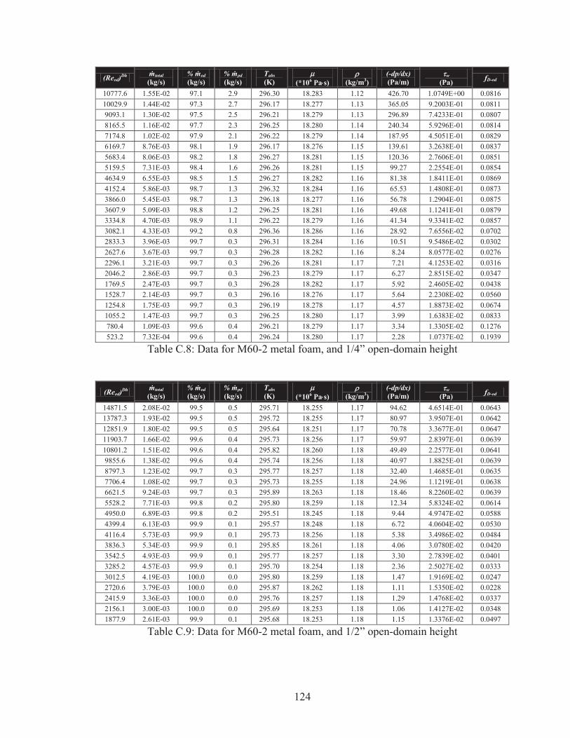
124
(Reod)Dh total (kg/s)
% od (kg/s)
% pd (kg/s)
Tabs (K)
(*106 Pa s)
(kg/m3)
(-dp/dx) (Pa/m)
w (Pa)
fD-od
10777.6 1.55E-02 97.1 2.9 296.30 18.283 1.12 426.70 1.0749E+00 0.0816 10029.9 1.44E-02 97.3 2.7 296.17 18.277 1.13 365.05 9.2003E-01 0.0811 9093.1 1.30E-02 97.5 2.5 296.21 18.279 1.13 296.89 7.4233E-01 0.0807 8165.5 1.16E-02 97.7 2.3 296.25 18.280 1.14 240.34 5.9296E-01 0.0814 7174.8 1.02E-02 97.9 2.1 296.22 18.279 1.14 187.95 4.5051E-01 0.0829 6169.7 8.76E-03 98.1 1.9 296.17 18.276 1.15 139.61 3.2638E-01 0.0837 5683.4 8.06E-03 98.2 1.8 296.27 18.281 1.15 120.36 2.7606E-01 0.0851 5159.5 7.31E-03 98.4 1.6 296.26 18.281 1.15 99.27 2.2554E-01 0.0854 4634.9 6.55E-03 98.5 1.5 296.27 18.282 1.16 81.38 1.8411E-01 0.0869 4152.4 5.86E-03 98.7 1.3 296.32 18.284 1.16 65.53 1.4808E-01 0.0873 3866.0 5.45E-03 98.7 1.3 296.18 18.277 1.16 56.78 1.2904E-01 0.0875 3607.9 5.09E-03 98.8 1.2 296.25 18.281 1.16 49.68 1.1241E-01 0.0879 3334.8 4.70E-03 98.9 1.1 296.22 18.279 1.16 41.34 9.3341E-02 0.0857 3082.1 4.33E-03 99.2 0.8 296.36 18.286 1.16 28.92 7.6556E-02 0.0702 2833.3 3.96E-03 99.7 0.3 296.31 18.284 1.16 10.51 9.5486E-02 0.0302 2627.6 3.67E-03 99.7 0.3 296.28 18.282 1.16 8.24 8.0577E-02 0.0276 2296.1 3.21E-03 99.7 0.3 296.26 18.281 1.17 7.21 4.1253E-02 0.0316 2046.2 2.86E-03 99.7 0.3 296.23 18.279 1.17 6.27 2.8515E-02 0.0347 1769.5 2.47E-03 99.7 0.3 296.28 18.282 1.17 5.92 2.4605E-02 0.0438 1528.7 2.14E-03 99.7 0.3 296.16 18.276 1.17 5.64 2.2308E-02 0.0560 1254.8 1.75E-03 99.7 0.3 296.19 18.278 1.17 4.57 1.8873E-02 0.0674 1055.2 1.47E-03 99.7 0.3 296.25 18.280 1.17 3.99 1.6383E-02 0.0833 780.4 1.09E-03 99.6 0.4 296.21 18.279 1.17 3.34 1.3305E-02 0.1276 523.2 7.32E-04 99.6 0.4 296.24 18.280 1.17 2.28 1.0737E-02 0.1939
Table C.8: Data for M60-2 metal foam, and 1/4” open-domain height
(Reod)Dh total (kg/s)
% od (kg/s)
% pd (kg/s)
Tabs (K)
(*106 Pa s)
(kg/m3)
(-dp/dx) (Pa/m)
w (Pa)
fD-od
14871.5 2.08E-02 99.5 0.5 295.71 18.255 1.17 94.62 4.6514E-01 0.0643 13787.3 1.93E-02 99.5 0.5 295.72 18.255 1.17 80.97 3.9507E-01 0.0642 12851.9 1.80E-02 99.5 0.5 295.64 18.251 1.17 70.78 3.3677E-01 0.0647 11903.7 1.66E-02 99.6 0.4 295.73 18.256 1.17 59.97 2.8397E-01 0.0639 10801.2 1.51E-02 99.6 0.4 295.82 18.260 1.18 49.49 2.2577E-01 0.0641 9855.6 1.38E-02 99.6 0.4 295.74 18.256 1.18 40.97 1.8825E-01 0.0639 8797.3 1.23E-02 99.7 0.3 295.77 18.257 1.18 32.40 1.4685E-01 0.0635 7706.4 1.08E-02 99.7 0.3 295.73 18.255 1.18 24.96 1.1219E-01 0.0638 6621.5 9.24E-03 99.7 0.3 295.89 18.263 1.18 18.46 8.2260E-02 0.0639 5528.2 7.71E-03 99.8 0.2 295.80 18.259 1.18 12.34 5.8324E-02 0.0614 4950.0 6.89E-03 99.8 0.2 295.51 18.245 1.18 9.44 4.9747E-02 0.0588 4399.4 6.13E-03 99.9 0.1 295.57 18.248 1.18 6.72 4.0604E-02 0.0530 4116.4 5.73E-03 99.9 0.1 295.73 18.256 1.18 5.38 3.4986E-02 0.0484 3836.3 5.34E-03 99.9 0.1 295.85 18.261 1.18 4.06 3.0780E-02 0.0420 3542.5 4.93E-03 99.9 0.1 295.77 18.257 1.18 3.30 2.7839E-02 0.0401 3285.2 4.57E-03 99.9 0.1 295.70 18.254 1.18 2.36 2.5027E-02 0.0333 3012.5 4.19E-03 100.0 0.0 295.80 18.259 1.18 1.47 1.9169E-02 0.0247 2720.6 3.79E-03 100.0 0.0 295.87 18.262 1.18 1.11 1.5350E-02 0.0228 2415.9 3.36E-03 100.0 0.0 295.76 18.257 1.18 1.29 1.4768E-02 0.0337 2156.1 3.00E-03 100.0 0.0 295.69 18.253 1.18 1.06 1.4127E-02 0.0348 1877.9 2.61E-03 99.9 0.1 295.68 18.253 1.18 1.15 1.3376E-02 0.0497
Table C.9: Data for M60-2 metal foam, and 1/2” open-domain height

125
(Reod)Dh total (kg/s)
% od (kg/s)
% pd (kg/s)
Tabs (K)
(*106 Pa s)
(kg/m3)
(-dp/dx) (Pa/m)
w (Pa)
fD-od
4171.4 9.27E-03 62.7 37.3 296.17 18.277 1.11 1336.71 1.2220E+00 0.0922 3789.4 8.40E-03 62.8 37.2 296.20 18.278 1.12 1115.55 1.0409E+00 0.0942 3500.1 7.74E-03 63.0 37.0 296.23 18.280 1.13 964.71 9.0918E-01 0.0961 3185.3 7.02E-03 63.2 36.8 296.24 18.280 1.14 809.90 7.7581E-01 0.0981 2877.5 6.32E-03 63.5 36.5 296.24 18.280 1.15 674.14 6.5738E-01 0.1006 2574.3 5.63E-03 63.7 36.3 296.24 18.280 1.15 554.43 5.4431E-01 0.1040 2417.8 5.27E-03 64.0 36.0 296.30 18.283 1.16 494.88 4.8875E-01 0.1054 2270.1 4.93E-03 64.2 35.8 296.33 18.284 1.16 441.94 4.3581E-01 0.1070 2108.6 4.56E-03 64.5 35.5 296.34 18.285 1.16 388.64 3.8730E-01 0.1093 1950.9 4.19E-03 64.8 35.2 296.27 18.281 1.16 338.20 3.4202E-01 0.1115 1792.6 3.84E-03 65.1 34.9 296.22 18.279 1.17 293.44 2.9732E-01 0.1148 1644.3 3.49E-03 65.6 34.4 296.22 18.279 1.17 250.76 2.5812E-01 0.1168 1496.8 3.15E-03 66.2 33.8 296.23 18.280 1.17 211.40 2.2177E-01 0.1190 1339.8 2.78E-03 67.1 32.9 296.20 18.278 1.17 172.51 1.8823E-01 0.1214 1180.2 2.41E-03 68.1 31.9 296.24 18.280 1.17 136.76 1.5362E-01 0.1242 1004.1 2.02E-03 69.3 30.7 296.13 18.275 1.18 103.65 1.1947E-01 0.1303 868.8 1.71E-03 70.8 29.2 296.11 18.274 1.18 79.14 9.4705E-02 0.1330 694.7 1.32E-03 73.1 26.9 296.08 18.272 1.18 52.72 6.6139E-02 0.1387 574.1 1.07E-03 74.6 25.4 296.18 18.277 1.18 38.63 4.8492E-02 0.1488 400.2 7.12E-04 78.3 21.7 296.17 18.277 1.18 20.67 2.9278E-02 0.1639 239.5 4.27E-04 78.1 21.9 296.20 18.278 1.18 12.17 1.9338E-02 0.2695 78.6 1.42E-04 76.9 23.1 296.19 18.278 1.18 4.12 9.8241E-03 0.8484
Table C.10: Data for ERG40-1 metal foam, and 1/8” open-domain height
(Reod)Dh total (kg/s)
% od (kg/s)
% pd (kg/s)
Tabs (K)
(*106 Pa s)
(kg/m3)
(-dp/dx) (Pa/m)
w (Pa)
fD-od
9172.4 1.52E-02 84.0 16.0 296.49 18.292 1.12 751.73 1.1410E+00 0.1035 8650.6 1.43E-02 84.2 15.8 296.43 18.289 1.13 665.53 1.0048E+00 0.1035 7826.5 1.29E-02 84.6 15.4 296.49 18.292 1.14 542.28 8.2063E-01 0.1036 7047.8 1.16E-02 84.9 15.1 296.49 18.292 1.14 439.88 6.7693E-01 0.1042 6220.1 1.01E-02 85.4 14.6 296.50 18.293 1.15 343.46 5.3276E-01 0.1050 5358.4 8.68E-03 86.0 14.0 296.51 18.293 1.15 257.30 4.0374E-01 0.1064 4948.7 7.99E-03 86.4 13.6 296.47 18.291 1.16 221.40 3.4862E-01 0.1076 4523.9 7.27E-03 86.8 13.2 296.52 18.293 1.16 186.03 2.9489E-01 0.1084 4070.4 6.50E-03 87.2 12.8 296.50 18.292 1.16 153.09 2.4525E-01 0.1104 3662.8 5.82E-03 87.7 12.3 296.48 18.291 1.16 125.41 2.0423E-01 0.1119 3415.1 5.40E-03 88.1 11.9 296.46 18.291 1.16 109.63 1.8337E-01 0.1127 3177.7 5.01E-03 88.4 11.6 296.48 18.292 1.16 96.49 1.6226E-01 0.1146 2970.2 4.67E-03 88.7 11.3 296.49 18.292 1.17 85.49 1.4393E-01 0.1163 2752.7 4.31E-03 89.0 11.0 296.49 18.292 1.17 74.60 1.2594E-01 0.1182 2526.7 3.95E-03 89.3 10.7 296.49 18.292 1.17 65.53 1.1001E-01 0.1234 2287.2 3.56E-03 89.5 10.5 296.47 18.291 1.17 56.75 9.3029E-02 0.1304 2055.1 3.19E-03 89.9 10.1 296.53 18.294 1.17 47.11 7.6987E-02 0.1342 1834.0 2.82E-03 90.5 9.5 296.50 18.293 1.17 38.30 6.3441E-02 0.1370 1602.5 2.45E-03 91.2 8.8 296.47 18.291 1.17 30.21 5.0903E-02 0.1417 1384.0 2.10E-03 92.1 7.9 296.46 18.291 1.17 22.65 3.9555E-02 0.1425 1152.1 1.73E-03 92.8 7.2 296.51 18.293 1.17 16.67 2.9104E-02 0.1513 965.4 1.43E-03 93.8 6.2 296.49 18.292 1.17 11.57 2.2277E-02 0.1497 744.4 1.09E-03 95.6 4.4 296.51 18.293 1.17 6.06 1.5471E-02 0.1319 497.8 7.22E-04 96.1 3.9 296.50 18.292 1.17 3.56 1.0152E-02 0.1733
Table C.11: Data for ERG40-1 metal foam, and 1/4” open-domain height
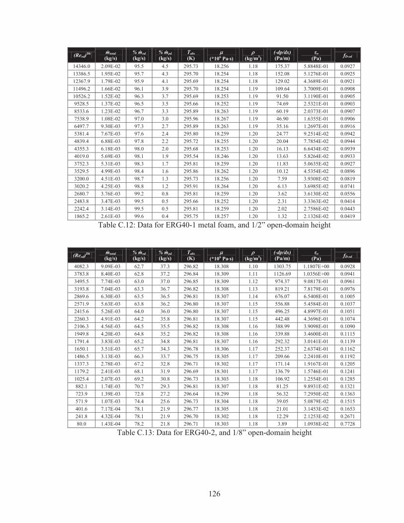
126
(Reod)Dh total (kg/s)
% od (kg/s)
% pd (kg/s)
Tabs (K)
(*106 Pa s)
(kg/m3)
(-dp/dx) (Pa/m)
w (Pa)
fD-od
14346.0 2.09E-02 95.5 4.5 295.73 18.256 1.18 175.37 5.8848E-01 0.0927 13386.5 1.95E-02 95.7 4.3 295.70 18.254 1.18 152.08 5.1276E-01 0.0925 12367.9 1.79E-02 95.9 4.1 295.69 18.254 1.18 129.02 4.3689E-01 0.0921 11496.2 1.66E-02 96.1 3.9 295.70 18.254 1.19 109.64 3.7009E-01 0.0908 10526.2 1.52E-02 96.3 3.7 295.69 18.253 1.19 91.50 3.1190E-01 0.0905 9528.5 1.37E-02 96.5 3.5 295.66 18.252 1.19 74.69 2.5321E-01 0.0903 8533.6 1.23E-02 96.7 3.3 295.89 18.263 1.19 60.19 2.0373E-01 0.0907 7538.9 1.08E-02 97.0 3.0 295.96 18.267 1.19 46.90 1.6355E-01 0.0906 6497.7 9.30E-03 97.3 2.7 295.89 18.263 1.19 35.16 1.2697E-01 0.0916 5381.4 7.67E-03 97.6 2.4 295.80 18.259 1.20 24.77 9.2514E-02 0.0942 4839.4 6.88E-03 97.8 2.2 295.72 18.255 1.20 20.04 7.7854E-02 0.0944 4355.3 6.18E-03 98.0 2.0 295.68 18.253 1.20 16.13 6.6434E-02 0.0939 4019.0 5.69E-03 98.1 1.9 295.54 18.246 1.20 13.63 5.8264E-02 0.0933 3752.3 5.31E-03 98.3 1.7 295.81 18.259 1.20 11.83 5.0635E-02 0.0927 3529.5 4.99E-03 98.4 1.6 295.86 18.262 1.20 10.12 4.5354E-02 0.0896 3200.0 4.51E-03 98.7 1.3 295.73 18.256 1.20 7.59 3.9308E-02 0.0819 3020.2 4.25E-03 98.8 1.2 295.91 18.264 1.20 6.13 3.6985E-02 0.0741 2680.7 3.76E-03 99.2 0.8 295.81 18.259 1.20 3.62 3.6130E-02 0.0556 2483.8 3.47E-03 99.5 0.5 295.66 18.252 1.20 2.31 3.3363E-02 0.0414 2242.4 3.14E-03 99.5 0.5 295.81 18.259 1.20 2.02 2.7586E-02 0.0443 1865.2 2.61E-03 99.6 0.4 295.75 18.257 1.20 1.32 2.1326E-02 0.0419
Table C.12: Data for ERG40-1 metal foam, and 1/2” open-domain height
(Reod)Dh total (kg/s)
% od (kg/s)
% pd (kg/s)
Tabs (K)
(*106 Pa s)
(kg/m3)
(-dp/dx) (Pa/m)
w (Pa)
fD-od
4082.3 9.09E-03 62.7 37.3 296.82 18.308 1.10 1303.75 1.1807E+00 0.0928 3783.8 8.40E-03 62.8 37.2 296.84 18.309 1.11 1126.69 1.0356E+00 0.0941 3495.5 7.74E-03 63.0 37.0 296.85 18.309 1.12 974.37 9.0817E-01 0.0961 3193.8 7.04E-03 63.3 36.7 296.82 18.308 1.13 819.21 7.8179E-01 0.0976 2869.6 6.30E-03 63.5 36.5 296.81 18.307 1.14 676.07 6.5408E-01 0.1005 2571.9 5.63E-03 63.8 36.2 296.80 18.307 1.15 556.88 5.4584E-01 0.1037 2415.6 5.26E-03 64.0 36.0 296.80 18.307 1.15 496.25 4.8997E-01 0.1051 2260.3 4.91E-03 64.2 35.8 296.81 18.307 1.15 442.48 4.3696E-01 0.1074 2106.3 4.56E-03 64.5 35.5 296.82 18.308 1.16 388.99 3.9098E-01 0.1090 1949.8 4.20E-03 64.8 35.2 296.82 18.308 1.16 339.88 3.4600E-01 0.1115 1791.4 3.83E-03 65.2 34.8 296.81 18.307 1.16 292.32 3.0141E-01 0.1139 1650.1 3.51E-03 65.7 34.3 296.78 18.306 1.17 252.37 2.6374E-01 0.1162 1486.5 3.13E-03 66.3 33.7 296.75 18.305 1.17 209.66 2.2410E-01 0.1192 1337.3 2.78E-03 67.2 32.8 296.71 18.302 1.17 171.14 1.9167E-01 0.1205 1179.2 2.41E-03 68.1 31.9 296.69 18.301 1.17 136.79 1.5746E-01 0.1241 1025.4 2.07E-03 69.2 30.8 296.73 18.303 1.18 106.92 1.2554E-01 0.1285 882.1 1.74E-03 70.7 29.3 296.81 18.307 1.18 81.25 9.8931E-02 0.1321 723.9 1.39E-03 72.8 27.2 296.64 18.299 1.18 56.32 7.2950E-02 0.1363 571.9 1.07E-03 74.4 25.6 296.73 18.304 1.18 39.05 5.0879E-02 0.1515 401.6 7.17E-04 78.1 21.9 296.77 18.305 1.18 21.01 3.1453E-02 0.1653 241.8 4.32E-04 78.1 21.9 296.70 18.302 1.18 12.29 2.1253E-02 0.2671 80.0 1.43E-04 78.2 21.8 296.71 18.303 1.18 3.89 1.0938E-02 0.7728
Table C.13: Data for ERG40-2, and 1/8” open-domain height
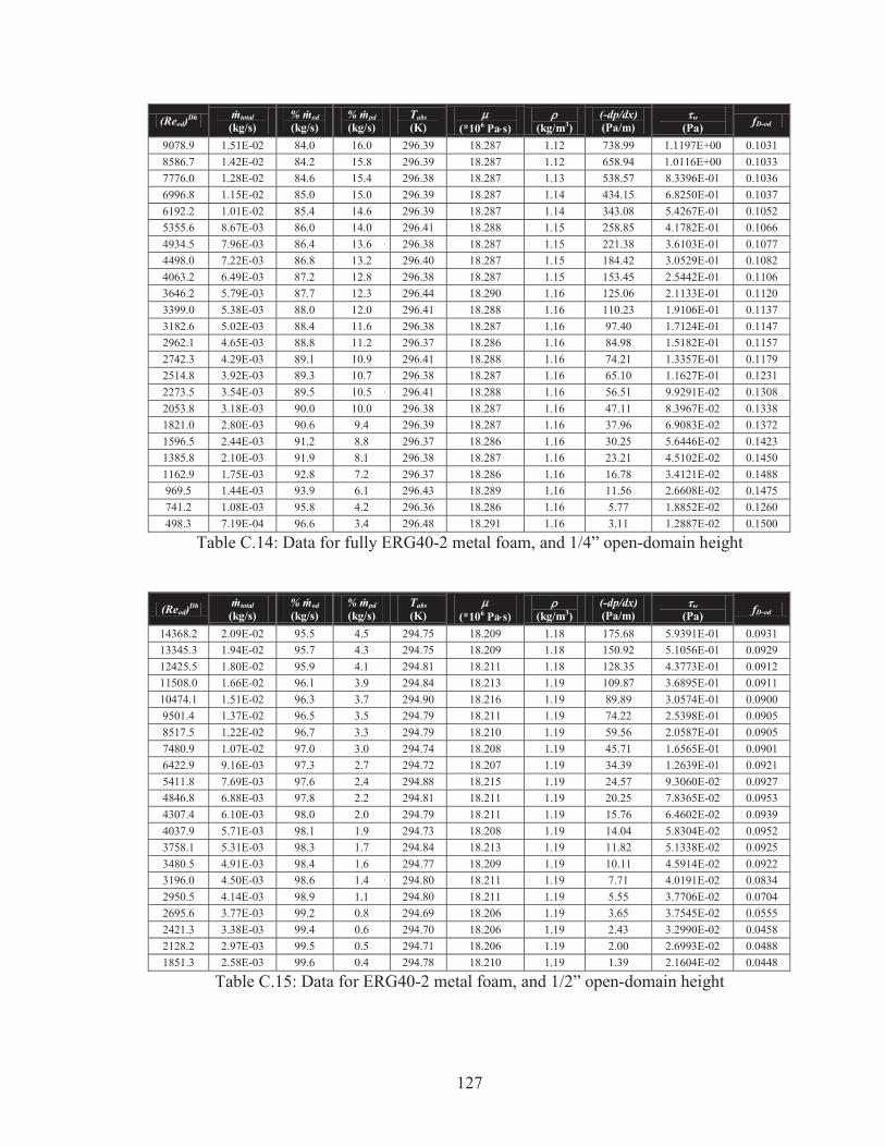
127
(Reod)Dh total (kg/s)
% od (kg/s)
% pd (kg/s)
Tabs (K)
(*106 Pa s)
(kg/m3)
(-dp/dx) (Pa/m)
w (Pa)
fD-od
9078.9 1.51E-02 84.0 16.0 296.39 18.287 1.12 738.99 1.1197E+00 0.1031 8586.7 1.42E-02 84.2 15.8 296.39 18.287 1.12 658.94 1.0116E+00 0.1033 7776.0 1.28E-02 84.6 15.4 296.38 18.287 1.13 538.57 8.3396E-01 0.1036 6996.8 1.15E-02 85.0 15.0 296.39 18.287 1.14 434.15 6.8250E-01 0.1037 6192.2 1.01E-02 85.4 14.6 296.39 18.287 1.14 343.08 5.4267E-01 0.1052 5355.6 8.67E-03 86.0 14.0 296.41 18.288 1.15 258.85 4.1782E-01 0.1066 4934.5 7.96E-03 86.4 13.6 296.38 18.287 1.15 221.38 3.6103E-01 0.1077 4498.0 7.22E-03 86.8 13.2 296.40 18.287 1.15 184.42 3.0529E-01 0.1082 4063.2 6.49E-03 87.2 12.8 296.38 18.287 1.15 153.45 2.5442E-01 0.1106 3646.2 5.79E-03 87.7 12.3 296.44 18.290 1.16 125.06 2.1133E-01 0.1120 3399.0 5.38E-03 88.0 12.0 296.41 18.288 1.16 110.23 1.9106E-01 0.1137 3182.6 5.02E-03 88.4 11.6 296.38 18.287 1.16 97.40 1.7124E-01 0.1147 2962.1 4.65E-03 88.8 11.2 296.37 18.286 1.16 84.98 1.5182E-01 0.1157 2742.3 4.29E-03 89.1 10.9 296.41 18.288 1.16 74.21 1.3357E-01 0.1179 2514.8 3.92E-03 89.3 10.7 296.38 18.287 1.16 65.10 1.1627E-01 0.1231 2273.5 3.54E-03 89.5 10.5 296.41 18.288 1.16 56.51 9.9291E-02 0.1308 2053.8 3.18E-03 90.0 10.0 296.38 18.287 1.16 47.11 8.3967E-02 0.1338 1821.0 2.80E-03 90.6 9.4 296.39 18.287 1.16 37.96 6.9083E-02 0.1372 1596.5 2.44E-03 91.2 8.8 296.37 18.286 1.16 30.25 5.6446E-02 0.1423 1385.8 2.10E-03 91.9 8.1 296.38 18.287 1.16 23.21 4.5102E-02 0.1450 1162.9 1.75E-03 92.8 7.2 296.37 18.286 1.16 16.78 3.4121E-02 0.1488 969.5 1.44E-03 93.9 6.1 296.43 18.289 1.16 11.56 2.6608E-02 0.1475 741.2 1.08E-03 95.8 4.2 296.36 18.286 1.16 5.77 1.8852E-02 0.1260 498.3 7.19E-04 96.6 3.4 296.48 18.291 1.16 3.11 1.2887E-02 0.1500
Table C.14: Data for fully ERG40-2 metal foam, and 1/4” open-domain height
(Reod)Dh total (kg/s)
% od (kg/s)
% pd (kg/s)
Tabs (K)
(*106 Pa s)
(kg/m3)
(-dp/dx) (Pa/m)
w (Pa)
fD-od
14368.2 2.09E-02 95.5 4.5 294.75 18.209 1.18 175.68 5.9391E-01 0.0931 13345.3 1.94E-02 95.7 4.3 294.75 18.209 1.18 150.92 5.1056E-01 0.0929 12425.5 1.80E-02 95.9 4.1 294.81 18.211 1.18 128.35 4.3773E-01 0.0912 11508.0 1.66E-02 96.1 3.9 294.84 18.213 1.19 109.87 3.6895E-01 0.0911 10474.1 1.51E-02 96.3 3.7 294.90 18.216 1.19 89.89 3.0574E-01 0.0900 9501.4 1.37E-02 96.5 3.5 294.79 18.211 1.19 74.22 2.5398E-01 0.0905 8517.5 1.22E-02 96.7 3.3 294.79 18.210 1.19 59.56 2.0587E-01 0.0905 7480.9 1.07E-02 97.0 3.0 294.74 18.208 1.19 45.71 1.6565E-01 0.0901 6422.9 9.16E-03 97.3 2.7 294.72 18.207 1.19 34.39 1.2639E-01 0.0921 5411.8 7.69E-03 97.6 2.4 294.88 18.215 1.19 24.57 9.3060E-02 0.0927 4846.8 6.88E-03 97.8 2.2 294.81 18.211 1.19 20.25 7.8365E-02 0.0953 4307.4 6.10E-03 98.0 2.0 294.79 18.211 1.19 15.76 6.4602E-02 0.0939 4037.9 5.71E-03 98.1 1.9 294.73 18.208 1.19 14.04 5.8304E-02 0.0952 3758.1 5.31E-03 98.3 1.7 294.84 18.213 1.19 11.82 5.1338E-02 0.0925 3480.5 4.91E-03 98.4 1.6 294.77 18.209 1.19 10.11 4.5914E-02 0.0922 3196.0 4.50E-03 98.6 1.4 294.80 18.211 1.19 7.71 4.0191E-02 0.0834 2950.5 4.14E-03 98.9 1.1 294.80 18.211 1.19 5.55 3.7706E-02 0.0704 2695.6 3.77E-03 99.2 0.8 294.69 18.206 1.19 3.65 3.7545E-02 0.0555 2421.3 3.38E-03 99.4 0.6 294.70 18.206 1.19 2.43 3.2990E-02 0.0458 2128.2 2.97E-03 99.5 0.5 294.71 18.206 1.19 2.00 2.6993E-02 0.0488 1851.3 2.58E-03 99.6 0.4 294.78 18.210 1.19 1.39 2.1604E-02 0.0448
Table C.15: Data for ERG40-2 metal foam, and 1/2” open-domain height