experimental evidence on bank runs under partial deposit
TRANSCRIPT
HAL Id: hal-01510692https://hal-essec.archives-ouvertes.fr/hal-01510692
Preprint submitted on 19 Apr 2017
HAL is a multi-disciplinary open accessarchive for the deposit and dissemination of sci-entific research documents, whether they are pub-lished or not. The documents may come fromteaching and research institutions in France orabroad, or from public or private research centers.
L’archive ouverte pluridisciplinaire HAL, estdestinée au dépôt et à la diffusion de documentsscientifiques de niveau recherche, publiés ou non,émanant des établissements d’enseignement et derecherche français ou étrangers, des laboratoirespublics ou privés.
Experimental evidence on bank runs under partialdeposit insurance
Oana Peia, Radu Vranceanu
To cite this version:Oana Peia, Radu Vranceanu. Experimental evidence on bank runs under partial deposit insurance.2017. �hal-01510692�
EXPERIMENTAL EVIDENCE ON BANK RUNS UNDER PARTIAL DEPOSIT
INSURANCE
RESEARCH CENTER OANA PEIA, RADU VRANCEANU
ESSEC WORKING PAPER 1705
APRIL 2017
Experimental Evidence on Bank Runs
under Partial Deposit Insurance∗
Oana Peia† Radu Vranceanu‡
April 11, 2017
Abstract
This paper presents experimental evidence on depositor behavior under partial deposit
insurance schemes. In the experiment, the size of a deposit insurance fund cannot fully
cover all deposits and the level of insurance depends on the number of depositors running
on the bank. We show that this form of strategic uncertainty about deposit coverage ex-
erts a significant impact on the propensity to withdraw, and results in a large frequency of
bank runs. Runs are more likely when depositors have noisy information about the size of
the insurance fund and as the maximum coverage increases, in line with a risk-dominant
equilibrium selection mechanism. From a policy perspective, our results emphasize the
limits of underfunded deposit insurance schemes in preventing systemic banking crises.
Keywords: Bank runs, Deposit insurance, Risk dominance, Global games.
JEL Classification: G21; G02; C91; D83
∗We are grateful to Delphine Dubart for her help in organizing the experimental sessions. We would also
like to thank Kasper Roszbach, Panicos Demetriades, Nicolas Coeurdacier, Vittorio Larocca, Davide Romelli
and participants to the 7th International Conference of the French Association of Experimental Economics
(Cergy, 2016) for useful comments and suggestions. This project was funded by a research grant provided by
the ESSEC Foundation.†University College Dublin. E-mail: [email protected].‡ESSEC Business School and THEMA, 1 Av. Bernard Hirsch, 95000, Cergy, France. E-mail:
1

1 Introduction
Deposit insurance schemes are crucial elements of modern financial safety nets. Demirguc-
Kunt and Laeven (2013) find that 60% of countries worldwide have a form of explicit deposit
insurance scheme in place.1 Economic theory generally argues that a full and credible deposit
insurance can prevent mass depositor withdrawals and eliminate bank runs (Diamond and
Dybvig, 1983). However, the majority of deposit insurance schemes in Demirguc-Kunt and
Laeven’s (2013) sample is grossly underfunded: in more than half of the countries, the size
of the insurance fund is less than 50% of the total deposits that need to be covered (in a
third of the countries, it is less than 10%). While these partially funded schemes might be
effective in preventing runs on banks hit by idiosyncratic shocks, if the entire banking sector
is under distress, the fund cannot guarantee all banks’ liabilities. As a result, even holders
of insured deposits can suffer substantial losses. This perspective of a systemic banking crisis
could potentially increase the risk of runs at individual banks, despite the presence of deposit
insurance.2 Indeed, in recent years many bank runs occurred in countries with extensive
deposit insurance schemes in place: the UK in 2008 (Northern Rock), the Netherlands in 2009
(DSB Bank), Latvia in 2012 (Swedbank), Bulgaria in 2014 (two banks), the systemic bank
run in Cyprus in 2013, as well as the “slow moving run” on deposits in Greece between 2010
and 2012.
These recent events call into question the effectiveness of deposit insurance schemes in allevi-
ating the risk of deposit withdrawals, particularly when the banking sector is hit by a common
shock.3 In this paper, we propose a laboratory experiment to study depositors’ behavior in
situations when the resources available in the insurance fund do not cover the total amount
of insured deposits in the banking sector, i.e. the deposit coverage is partial. In this context,
depositors face a strategic uncertainty about the deposit coverage, which depends on the size
of the insurance fund and the total number of depositors running on the bank.
In the experiment, five subjects play the role of depositors at a bank for ten identical rounds.
At the beginning of each round, they each receive a deposit and must decide whether to keep
their funds in the bank until the end of the round or withdraw them. The payoff depends on
1The source of funding and deposit coverage ratio varies markedly across countries. For example, thecoverage limit ranges from a low of $406 in Moldova to a high of $1.5 million in Thailand.
2Several empirical studies that look at the cross-country effects of financial safety nets provide evidence inthis direction. For example, Demirguc-Kunt and Detragiache (2002) find that explicit deposit insurance tendsto be detrimental to bank stability whenever the coverage is extensive, the insurance scheme is run by thegovernment and the institutional environment is weak. Similarly, Hoggarth, Jackson and Nier (2005) show thatcountries with explicit unlimited insurance are ex-ante more likely to experience a banking crisis. This evidencesuggests that depositors might anticipate that governments will not commit to the policy intervention ex-post,especially in cases of system-wide bank distress, thus increasing the probability of runs ex-ante.
3Our analysis pertains to cases in which the entire banking sector is in distress, such that the crisis is systemic.However, we do not address issues of contagion among banks (see Kaufman and Scott, 2003; Georg, 2013).
2
individual decisions, as well as the decisions of others. If only two or less depositors decide to
withdraw, those who leave their funds in the bank receive a substantial return. However, if
three or more depositors withdraw, we assume a bank run is under way. When such runs occur,
the bank fails and it can no longer repay depositors. As a result, depositors are compensated by
a deposit insurance fund, whose size is randomly drawn in each round. If the size of this fund
is large enough, depositors who withdraw can recover their initial deposit in full. Otherwise,
the fund is equally split between those who withdraw. Those who wait get nothing in case of
bank failure. This is a typical coordination game with strategic complementarities, similar to
the classical bank run game in Diamond and Dybvig (1983). The game has two pure-strategy
equilibria: (i) a payoff-dominant equilibrium where all players choose the “wait” strategy and
(ii) a bank-run equilibrium in which all players choose the “withdraw” strategy. Given the
multiplicity of equilibria of such coordination games, we employ two equilibrium refinements
to characterize the aggregate behavior of players. These are modeled in two experimental
treatments related to the type of information depositors receive about the deposit insurance
fund.
In a first condition, subjects play the wait/withdraw game under a perfect information setting,
in which they observe the actual size of the deposit insurance fund in each round. We em-
ploy a well-known equilibrium refinement, defined as risk-dominance in Harsanyi and Selten
(1988), to characterize the optimal strategies of players. In a second condition, we consider
a heterogeneous information variant of this game in which individuals only receive a noisy,
idiosyncratic signal about the size of the deposit insurance fund in each round. We employ
a global-games equilibrium refinement in this set-up. Carlsson and Van Damme (1993b) and
Morris and Shin (1998) show that such coordination games present a single “threshold equi-
librium” in which players pick the strategy that coincides with the risk-dominance criterion,
even when the payoff-dominant one is available. We find that players’ aggregate behavior in
each of the two treatments is consistent with these equilibrium selection criteria.4
Our main experimental result consists in showing that bank runs occur quite often, in a spon-
taneous way, despite the significantly higher payoff of the “wait” equilibrium. We refer to
a “bank run” as a situation in which more than two depositors withdraw and the deposit
insurance scheme must compensate depositors. Depending on the treatment, the frequency
of runs ranges from 2.5% to 45% of the cases and is significantly higher in the heterogeneous
information case compared to the perfect information one. Our results thus suggest that un-
certainty about the coverage of deposit insurance exerts a significant impact on the propensity
to withdraw and is an important trigger of bank runs. We analyze individual behavior and
show that a majority of players resort to “threshold strategies”, i.e., there is cut-off value of
4Several experimental papers have also shown that this threshold equilibrium is a valid characterizationof players’ behavior in various global games frameworks (Heinemann, Nagel and Ockenfels, 2004; Heinemann,Nagel and Ockenfels, 2009).
3
the size of the deposit insurance fund around which they switch between waiting and with-
drawing. Thus, using the two equilibrium refinements, we can characterize a fairly predictable
equilibrium behavior.
In both conditions, the frequency of participants who withdraw is increasing in the size of the
deposit insurance fund. This is in line with a risk-dominant equilibrium selection as the payoff
from playing the “safe” action, i.e. withdraw, is increasing with the size of the fund. Thus,
a very low deposit insurance actually reduces the probability of runs, as the expected payoff
from withdrawing is very low.5 At the same time, for very high levels of deposit insurance,
depositors are more prone withdraw, as the payoff from the “safe” option is high. From a
policy perspective, this suggests that a large, but partial deposit insurance level can actually be
detrimental to bank stability, particularly when the banking sector is hit by a common shock.
Our experimental results thus provide an alternative explanation to the empirical evidence
that looks at systemic banking crises and associates an extensive deposit coverage with a
higher ex-ante probability of bank distress (Demirguc-Kunt and Detragiache, 2002; Hoggarth
et al., 2005). We show that excessive risk-taking by banks might not be the only channel to
explain this higher risk of bank runs, as an extensive insurance might also prompt depositors
to withdraw, especially if they are uncertain about the level of deposit coverage. Thus, while
deposit insurance schemes can be an efficient way to contain runs at individual banks, they
might amplify or accelerate a systemic crisis.
These results bring new evidence to a growing body of literature that studies bank runs in
an experimental setting.6 Generally, such studies generate panic-based runs in the labora-
tory by (i) forcing some of the subjects to withdraw early (Madies, 2006; Kiss, Rodriguez-
Lara and Rosa-Garcıa, 2012; Garratt and Keister, 2009; Kiss, Rodriguez-Lara and Rosa-
Garcia, 2014); (ii) introducing uncertainty about banks’ returns and observability of actions
(Schotter and Yorulmazer, 2009; Brown, Trautmann and Vlahu, 2016; Chakravarty, Fonseca
and Kaplan, 2014) or (iii) varying the coordination parameter needed for the payoff-dominant
equilibrium to occur (Arifovic, Hua Jiang and Xu, 2013). For example, Garratt and Keis-
ter (2009) use a payoff structure similar to ours, but force some players to withdraw early.
However, in a treatment with no forced withdrawals, they find no evidence of runs and show
that players always coordinate on the payoff-dominant equilibrium. At difference with these
studies, our setting does not require any “exogenous” triggers of runs. We show that the
strategic uncertainty about the coverage provided by the deposit insurance fund suffices to
generate runs in the laboratory.
5This is in line with the results of other coordination games such as minimum effort experiments. Brandtsand Cooper (2006) show that a lower attractiveness of the safe action relative to the risky action leads to ahigher occurrence of the Pareto-optimal equilibrium.
6For surveys on applying experimental methods to macroeconomic issues including banking crises, see Duffy(2014), Cornand and Heinemann (2014) and Dufwenberg (2015).
4

Several experimental papers also explicitly consider the effects of deposit insurance on the
probability of panic-based runs. Madies (2006) studies the effectiveness of partial insurance
schemes in a standard Diamond and Dybvig bank run setting. He finds no link between the
levels of insurance and subjects’ propensity to withdraw. Schotter and Yorulmazer (2009),
in an experiment with multiple withdrawal opportunities, find that insurance postpones the
time of withdrawal, hence slowing down the bank run. Kiss et al. (2012) find that deposit
insurance decreases the probability of a run, but this effect disappears when depositors can
observe the number of withdrawals that took place before theirs. However, in all these settings,
depositors’ payoff from withdrawing is certain, i.e., they are informed about the coverage of
deposit insurance in the case of a run. We consider an alternative setting in which the exact
size of deposit coverage is uncertain, as it depends on the number of subjects running on
the bank. We show that this uncertainty is a strong propagator of runs, the more so, when
subjects receive noisy information.
The remainder of this paper is organized as follows. The next section introduces our ex-
perimental design. Section 3 sketches a theoretical and numerical solution to the depositor
decision problem. Section 4 presents the experimental results, while Section 5 concludes.
2 Experimental design
We conducted six experimental sessions at the ESSEC Experimental Lab between May 2015
and June 2016 with 120 participants recruited among the student population of ESSEC Busi-
ness School. Each session involved 20 subjects who participated in 10 successive decision
rounds. In each session, subjects were divided into groups of five, which represented the pool
of depositors at a bank. Groups were rematched after every round in a typical stranger de-
sign. All interactions were computerized using the z-Tree package (Fischbacher, 2007) and the
anonymity of the subjects was guaranteed.
At the beginning of each decision round, each player receives an endowment of 10 Euro as a
deposit in a bank. Depositors choose between two actions: “withdraw” their deposit or “wait”
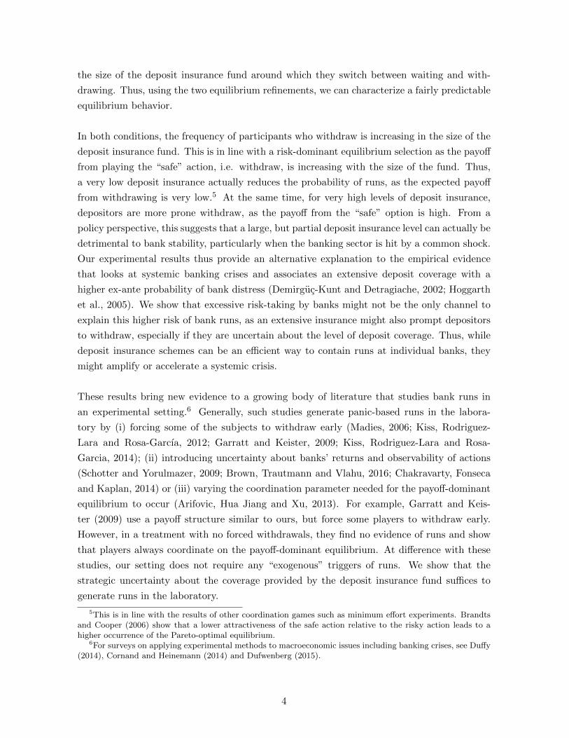
until the end of the round, when they can potentially receive a higher payoff. Table 1 presents
the structure of payments. The final payoff at the end of each round depends on the number of
depositors who decide to withdraw their funds from the bank. Specifically, if everyone decides
to wait, at the end of the round, the initial deposit becomes R, with R > 10. Following
Diamond and Dybvig (1983), we assume a strategic complementarity in actions, such that, as
long as a bank run does not occur, the return of those who wait decreases smoothly with the
number of withdrawals (see Table 1). Furthermore, subjects are informed that the bank is
able to absorb at most two withdrawals before it liquidates all its assets (we implicitly assume
5
that the bank cannot fire-sale assets). Thus, if two depositors or less withdraw, the bank can
repay their deposit of 10 Euro, in full. However, if three or more withdraw, the bank’s liquidity
reserves are depleted and depositors are covered by the deposit insurance fund, whose size is
denoted by D. Once a bank run is under way, depositors who wait get nothing.
Table 1: Promised returns
Number of depositors who withdraw Payoff if withdraw Payoff if wait
0 - R1 10 R-12 10 R-23 minimum{D/3, 10} -4 minimum{D/4, 10} -5 minimum{D/5, 10} -
In each round, the size of the deposit insurance fund changes and is randomly draw by the
computer from the set of integers uniformly distributed over [0,50]. Those who withdraw
receive the minimum between D/n and 10, where n ∈ {3, 4, 5} is the number of depositors
withdrawing (see Table 1). This implies that the deposit insurance fund is evenly split among
depositors who withdraw and, naturally, it will not reimburse more than the initial deposit.
This payoff structure reveals the strategic complementarity of players’ actions. For n ≤ 2,
the more depositors wait, the higher the payoff from waiting. When n > 2, the bank fails
and subjects have a dominant action to withdraw. If all depositors withdraw, they each get
D/5 ≤ 10.7
The payment structure in Table 1 is similar to previous experimental tests of the classical
Diamond and Dybvig (1983) bank run model (see Madies, 2006; Garratt and Keister, 2009).
At difference, we assume that the amount depositors can recover in case of runs is no longer
fixed, but depends on the number of depositors also withdrawing. This makes the coverage
ratio of deposit insurance uncertain. Our main goal is to analyze if this uncertainty has an
impact on individuals’ ex-ante propensity to run. It should also be noted that, no other type
of uncertainty or exogenous trigger of runs is introduced in the coordination game.
We have performed six experimental sessions as detailed in Table 2. We consider a stan-
dard between-subjects design, with participants attending only one of the six experimental
7Note that the coordination threshold is set at 60%. This is a significantly lower requirement than inclassical coordination problems such as minimum effort games (Van Huyck, Battalio and Beil, 1990; 1991). Thebreakdown in coordination is common in these minimum effort games, as the deviation of a single participantis sufficient for the Pareto-dominant outcome not to prevail. In the context of bank-run models, Arifovic et al.(2013) explicitly test for the level of coordination required for the run to occur and show that whenever it isless than 50% (or more than 80%) subjects only play the payoff dominant (respectively run) equilibrium. Ourcoordination coefficient lies in the intermediate region where multiple equilibria are likely to occur.
6

Table 2: Experimental Sessions
Treatments Number of Students Date
Perfect information, Low return 20 January, 2016Perfect information, High return 40 February/June, 2016Heterogeneous information, Low return 20 May, 2015Heterogeneous information, High return 40 May, 2015/June 2016
sessions. The experiment has two main treatments. In the “Perfect information” treatment,
participants are informed about the size of the deposit insurance fund, D, in each round. In
the “Heterogeneous information” treatment, they receive idiosyncratic hints about the size of
the deposit insurance fund, which are uniformly distributed around the true value of D. We
performed three sessions under each treatment. Within each treatment, we considered two
variations of the maximum payoff attainable, R. Out of the six sessions, four have a “high”
return, RH = 16, and two a “low” return, RL = 14. We vary the level of the return, R, to
test whether changes in the payoff-dominant outcome affect behavior in any way. Previous
research has shown that changing the level of risk-dominance affects equilibrium outcomes,
while changes in the level of payoff-dominance do not (see Schmidt, Shupp, Walker and Os-
trom, 2003).
In two of the four heterogeneous information treatments, subjects were also asked to guess
the number of withdrawals before they make their decision. This guess was incentivized, such
that a better estimation of the number of withdrawals allowed subjects to increase their payoff
by a maximum of 5 Euro.8
At the end of each of the 10 rounds, subjects learn their payoff and how many depositors have
withdrawn in that round. In the heterogeneous information treatments they are also informed
about the true value of D. At the end of the experiment, one of the ten rounds is selected
randomly to determine the subjects’ remuneration from the experiment, to which a 5 Euro
participation fee is added.9 On average, participants earned 18.68 Euro and sessions lasted
around 50 minutes, including the time to read out loud the instructions.
8The extra payment was according to the formula: 5/(1 + error), where error is the absolute differencebetween their guess and the actual number of withdrawals.
9Previous experiments in coordination have found that random payments give the higher possible impact ofrisk aversion and induce players to avoid hedging (Heinemann et al., 2004).
7
3 Theoretical predictions
This section describes the equilibrium selection theories employed to characterize aggregate
behavior and computes numerically the solutions they imply.
3.1 Perfect information setting
In the perfect information setting, subjects are informed at the beginning of each round about
the size of the deposit insurance fund, D. This game has two Nash equilibria in pure strategies.
In the payoff-dominant equilibrium, all depositors choose the “wait” strategy and receive the
large payoff, R > 10. An individual depositor who unilaterally deviates (plays withdraw)
would get at most 10 Euro. In the second equilibrium, all players choose the “withdraw”
strategy and receive D/5. Since the bank is now bankrupt, a player who unilaterally deviates
(plays wait), would get zero. The first equilibrium is Pareto-dominant, but it is risky insofar
as it requires a majority of players to coordinate on leaving their funds in the bank.
One intuitive equilibrium selection theory for such games with two Pareto-ranked equilibria
relies on the concept of risk dominance introduced by Harsanyi and Selten (1988). In general,
this equilibrium selection criterion is tantamount to players choosing their “safe” strategy,
i.e., the strategy that minimize their losses should opponents deviate from their equilibrium
strategy. In games with two possible actions and symmetric payoffs, a player chooses the action
that maximizes his/her expected net gain, under the assumption that others play either action
with an equal probability.10 In our case, this concept implies that players should withdraw as
long as the expected utility from withdrawing is higher than the expected utility of leaving
the money in the bank.11 We proceed to compute these expected utilities in a multiple players
set-up following Heinemann et al. (2004).
Let n be the number of players who withdraw. Then the payoff from leaving the deposit in
the bank (wait) can be written as:
PayoffWAIT(n) =
R− n if n ≤ 2
0 if n > 2(1)
10Stahl and Wilson (1994) defines this type of behavior in which a player best responses to a uniform play byother players as a level-1 reasoning. They show that it characterizes around 60% of the population of subjectsconsidered.
11Carlsson and Van Damme (1993a) and Kim (1996) extend Harsanyi and Selten’s (1988) risk dominanceconcept to stag-hunt games with more than two players. They show that the threshold size of the safe payoff,above which players choose the risk-dominant equilibrium, differs when more than two players are involved.Here, we are interested in computing numerically the critical size of this safe payoff.
8
Thus, the expected payoff from waiting is the return obtained given that none, one or two of
the other depositors decide to withdraw. The probability that at most two other depositors
withdraw given that each subject withdraws with a probability of p = 50% can be represented
by the binomial probability function. We denote this binomial probability by B(n, 4, p), where
n is the number of the other 4 depositors who decide to withdraw, when each withdraws with
a probability p. Then the expected payoff from waiting is simply:
EPWAIT =4∑
n=0
B(n, 4, p)PayoffWAIT(n). (2)
Similarly, the payoff from withdrawing is 10 Euro, if the bank does not fail. However, if the
bank fails (n > 2), the deposit is covered as long as the deposit insurance fund has enough
funds to repay all the depositors who withdraw, i.e., if D ≥ 10n. Otherwise, each depositor
who withdraws gets an equal share of D, i.e., D/n. More precisely, this payoff is:
PayoffWITHDRAW(n) =
10 if n ≤ 2
10Prob[D ≥ 10n] + Dn Prob[D < 10n] if n > 2
(3)
As D is uniformly distributed over [0,50], this payoff is a linearly increasing function of D for all
n > 2. Same as before, the expected payoff from withdrawing is the return from withdrawing
given that none, one, two, three or four of the other depositors also withdraw:
EPWITHDRAW =
4∑n=0
B(n, 4, p)PayoffWITHDRAW(n). (4)
We show that there is a threshold deposit insurance, denoted by D, such that depositors are
indifferent between waiting or withdrawing, implicitly defined by the indifference condition:
4∑n=0
B(n, 4, p)PayoffWITHDRAW(n) =4∑
n=0
B(n, 4, p)PayoffWAIT(n) (5)
The risk-dominant equilibrium refinement thus suggests that players will withdraw for D > D,
as the expected payoff from choosing the “safe” strategy, i.e. to withdraw, is increasing in the
size of the deposit insurance fund. Similarly, for D < D, players choose to leave their money
in the bank, as the expected payoff from withdrawing is lower.
Solving equation (5) numerically, we obtain the thresholds D14 = 15.43 when R = 14 and
D16 = 25.45 for R = 16. Clearly, for D > D, the payoff-dominance and risk-dominance
selection criteria generate conflicting recommendations. Harsanyi and Selten (1988) posit
that the payoff dominant equilibrium should prevail if players “trust each other to play the
payoff dominant strategy”. However, how much players “trust” each other may depend on the
9

risk and payoff characteristics of the game. For example, Schmidt et al. (2003) find that, in
a 2-player coordination game, players’ willingness to trust others to play the payoff dominant
equilibrium is influenced by the size of the safe payoff. In our case, as well, the variability of
the safe payoff should make subjects more likely to play the “safe” option and withdraw when
D is relatively large, in line with a risk-dominant equilibrium selection.
In our framed experiment, a potential fear of bank runs should make subjects more eager
to play the risk-dominant strategy. This would induce them to withdraw for higher levels of
deposit insurance, as the payoff from the “safe” action is higher. In the context of real world
bank runs, this can be interpreted as situations when deposit coverage tends to be extensive,
yet, because the coverage is so high, depositors fear that the size of the fund might not be
large enough to cover all insured deposits.
3.2 Heterogeneous information setting
In this alternative setting, depositors are not informed about the value of D randomly drawn
in each round. Depositor i only receives a signal about the true size of D, which takes the
following form:
xi = D + εi, (6)
where D is uniformly distributed over [0, 50] and εi is an individual-specific noise also uniformly
distributed on the support [−10, 10]. Under this assumption, the problem can be solved as a
typical global game, where subjects play a “threshold strategy” and switch between actions
depending on the signal received (see Morris and Shin, 1998; Morris and Shin, 2001; Goldstein
and Pauzner, 2005). In particular, there exists a critical signal x∗ such that individuals
receiving a signal xi < x∗ will wait, and those receiving a signal xi > x∗, will withdraw. The
existence of threshold strategies rests on the idea that signals contain information not only
about the true size of D, but also about the signals that the other players receive. Consider
a player who receives a signal xi = 0, then he/she has a dominant action to choose action
“wait” as the expected payoff from withdrawing is lower (close to zero) regardless of the
actions of the other players. Using an iterated elimination of dominated actions, we can find
a threshold signal, x∗, below which the action “withdraw” is always dominated. Similarly, a
player receiving a signal close to xi = 50, should have a dominant action to withdraw, as he/she
obtains a safe payoff of (almost) 10 Euro. Again, iterated elimination of dominated strategies
shows that for signals above x∗, players have a dominant action to withdraw (see also Morris
and Shin, 2003; Goldstein, 2010). Note that the global games equilibrium refinement “forces”
players to choose the risk-dominant equilibrium, even when the payoff-dominant option is
10

available (Carlsson and Van Damme, 1993b).12
The equilibrium threshold, x∗, can be found by characterizing the expected utility of the
depositor who receives exactly the threshold signal x∗ and who is indifferent between with-
drawing and waiting. We thus proceed to compute the expected utility of this “pivotal” agent.
Let n be the number of players who withdraw. The expected utility from leaving the money
in the bank is the utility from waiting given that at most two people withdraw. The prob-
ability that at most two people withdraw, given that players withdraw when they receive a
signal above x∗, can be described by a binomial distribution, as in the perfect information
case. Denote by p the probability that a single player gets a signal above x∗ at state D, i.e.,
p = Prob[xi > x∗|D]. Then the expected payoff of waiting can be expressed as:
EPWAIT(x∗) =4∑
n=0
[1
2ε
∫ x∗+ε
x∗−εB(n, 4, p)PayoffWAIT(n)dD
], (7)
where B is the binomial probability function, while the PayoffWAIT function is the same as in
the perfect information case in Equation 1.13 Similarly, the expected payoff from withdrawing
is the gain given that none, one, two, three or four of the others also withdraw:
EPWITHDRAW(x∗) =4∑
n=0
[1
2ε
∫ x∗+ε
x∗−εB(n, 4, p)PayoffWITHDRAW(n)dD
], (8)
where PayoffWITHDRAW is given by Equation 3. Replacing p by Prob[xi > x∗|D∗] = 1−x∗−D+εε ,
we can compute the threshold signal, as the signal received by the depositor who is indifferent
between withdrawing and waiting: EPWITHDRAW(x∗) = EPWAIT(x∗).
The indifference equation:
4∑n=0
[1
2ε
∫ x∗+ε
x∗−εB(n, 4, p)PayoffWAIT(n)dD
]=
4∑n=0
[1
2ε
∫ x∗+ε
x∗−εB(n, 4, p)PayoffWITHDRAW(n)dD
]
implicitly defines the critical x∗.
The numerical solution to this indifference condition yields the critical thresholds x∗ = 10.23
for R = 14 and x∗ = 20.23 for R = 16, respectively.
12In binary-action games with two players, the global games solution and the risk-dominance criteria yieldthe same equilibrium threshold (Carlsson and Van Damme, 1993b; Heinemann et al., 2009). In games withmultiple players, both concepts give similar predictions. The difference is that the Harsanyi and Selten (1988)approach relies on some ad hoc assumption about expectations formation, typically in the form of an uniformprior, while the global games solution derives these expectations from fundamental assumptions about howplayers’ information is generated.
13Note that in expression 7 above, we acknowledge the fact that the ex-post distribution of D is uniform overthe interval [x∗ − ε, x∗ + ε].
11

So the two equilibrium selection refinements yield similar predictions, suggesting that players
pick the risk-dominant equilibrium and switch from leaving the money in the bank to with-
drawing when the value of the deposit insurance fund increases above a computed threshold.
4 Experimental results
4.1 Observed behavior
Table 3 summarizes the observed individual and group behavior across the six experimental
sessions conducted. We observe a significant proportion of withdrawals across most sessions
and treatments. On average, subjects chose to withdraw in approximately 24% of the cases,
leading to a proportion of bank runs, i.e., situations in which three or more depositors with-
draw, in 19% of the rounds. The number of withdrawals varies from 14% of the total number
of withdrawal opportunities in Session 2 to a high as 45% in Session 5. This also results in a
relatively high occurrence of bank runs. Runs occur from 3% of the cases to 45% of the total
number of bank runs possible in Session 5.
Table 3: Descriptive Statistics
Session Treatment % Withdrawals % Bank runs
S1 Perfect information - Low Return 19% 18%S2 Perfect information - High Return 14% 3%S3 Perfect information - High Return 24% 13%S4 Heterogeneous information - Low Return 22% 20%S5 Heterogeneous information - High Return 45% 45%S6 Heterogeneous information - High Return 19% 15%
The total number of observations per treatment is 200. The total number of possible bank runs per treatment
is 40 (10 rounds x 4 banks/round). Sessions S4, S5 also included an incentivized guess.
Notably, the occurrence of the payoff-dominant equilibrium where none of the depositors
withdraw is similar, ranging from 4% (in Session 5) to 22% of the cases (in Session 2). Thus,
the large majority of rounds experienced partial runs where three or more depositors choose
the withdraw strategy. We can therefore state the following first result:
RESULT 1. The frequency of individuals who choose the withdraw strategy is relatively
high and entails a large number of runs in most treatments.
Thus, the introduction of strategic uncertainty about the coverage of deposit insurance suffices
12

to lead to a significant breakdown in subjects’ coordination on the payoff-dominant outcome.
This result is contrasting with the results of Garratt and Keister (2009), who also study a 5
depositors bank with a similar payoff structure. At difference, whenever bank runs occur in
their experiment, the payoff from withdrawing is fixed and known a priori. In this setting,
they observe no bank runs and the occurrence of the payoff-dominant equilibrium in 100%
of the cases. They then resort to forced withdrawals to generate panic-based runs. In a
similar manner, previous bank run experiments also resort to “exogenous” triggers of runs
such as forcing some subjects to withdraw, allowing the observability of actions of those
who chose before the subject or varying the size of the coordination needed to achieve the
payoff-dominant equilibrium (for an overview of the literature, see Duffy, 2014). Classical
unframed coordination games in the laboratory also see mixed results. The early experiments
with minimum effort games by Van Huyck, Battalio and Beil (1990; 1991) largely suggested
that coordination failure is a common phenomena in the laboratory. However, in these games,
reaching the payoff-dominant equilibrium is extremely difficult, as deviations by a single player
cause a breakdown in coordination. Stag-hunt games, which are closer to the bank-run model
studied here, find largely mixed results depending of the attractiveness of the secure payoff or
the riskiness of the other choices (see Devetag and Ortmann, 2007).
Regarding the difference between our two main treatments, we observe a higher propensity
to withdraw in the heterogeneous information treatments for both the low and high return
settings. The Wilcoxon-Mann-Whitney test that the median number of withdrawals is the
same in the perfect vs heterogeneous information treatments is rejected at a 1% confidence
level (z = -6.982). Similarly, the statistical difference between the perfect vs heterogeneous
information treatments is present if we consider separately the low return RL = 14 treatments
(z= -3.24, p=0.0012) or the high return, RH = 16, ones (z= -6.443, p=0.0000). This suggests
a significantly higher propensity to run in the heterogeneous information treatment, regardless
of the size of the payoff-dominant return. Indeed, the size of R appears to have an ambiguous
effect on the number of withdrawals, as the high return treatments can have either a higher
or lower number of total withdrawals and bank runs in both the perfect and heterogeneous
information treatments (see Table 3). We can state that:
RESULT 2. The frequency of withdrawals (and runs) is significantly higher in the hetero-
geneous information compared to perfect information treatments.
This is in line with Heinemann et al. (2004) who provide the first experimental test of equi-
librium selection in global games and find that, in the perfect information setting, subjects
coordinate more often on the payoff-dominant equilibrium, compared to the heterogeneous
information one.
13

Figure 1: Average withdrawal rate across treatments
0.2
.4.6
Ave
rage
With
draw
al
[0−10] (10−20] (20−30] (30−40] (40−50]
Withdrawal rates across treatments
Perfect information Heterogeneous information
4.2 Deposit coverage and the number of withdrawals
Figure 1 presents the frequency of withdrawals across the distribution of D, in the per-
fect/heterogeneous information treatments. It shows the average withdrawal rate in each
treatment, by pooling observations for the low and high return scenarios. In line with the av-
erage results in Table 3, it can be observed that for each interval of D considered, the average
withdrawal rate is considerably higher under the heterogeneous information treatment com-
pared to the perfect information one. In other words, uncertainty about the level of deposit
insurance is associated with a higher withdrawal rate, at any level of the deposit insurance
fund. Moreover, we can clearly observe that the average number of withdrawals is increasing
in D (regardless of the information structure). This behavior is confirmed in Figure 2, which
plots locally weighted regressions of the total number of withdrawals per bank for different
realizations of D. These figures now consider the Low (R = 14) and High return (R = 16)
scenarios of each treatment separately. Consistent with previous results, the noisy signals
treatment is associated with a higher number of withdrawals, and the results appear similar
regardless of the value of R. We can establish the following result:
RESULT 3. Regardless of the information structure, the frequency of withdrawals is increas-
ing in the maximum deposit coverage ratio.
These results suggest that players’ strategies are in line with a risk-dominant equilibrium
14

01
23
4T
otal
With
draw
0 10 20 30 40 50D
Total withdrawal Heterogeneous informationPerfect information
bandwidth = .8
Low return R=14
01
23
45
Tot
alW
ithdr
aw
0 10 20 30 40 50D
Total withdrawal Heterogeneous informationPerfect information
bandwidth = .8
High return R=16
Figure 2: Locally weighted regressions of the total number of withdrawals for different real-izations of D
selection, following the theoretical arguments in Section 3. In the perfect information case,
we have argued that players would pick the withdraw strategy for higher values of D, as the
expected return from running on the bank increases with the size of the deposit insurance
fund. Similarly, in the heterogeneous information treatment, the global games equilibrium
refinement entails that depositors with signals above a threshold, have a dominant action to
withdraw.
These equilibrium refinements yield a solution which might appear counter-intuitive, as the
frequency of withdrawals increases in the size of the deposit insurance. However, this is a
natural outcome in our model, in which as a bank run is tantamount to a systemic failure
and triggers the use of the deposit insurance fund to cover depositors. As such, a higher level
of maximum coverage prompts participants to pick the safe strategy, i.e., to withdraw. On
the other hand, when the coverage is low, players prefer to coordinate on the risky strategy.
Thus, a high deposit insurance coverage can breed instability, as depositors rush to the bank
to recover their investment in full.
Overall, these results bring new evidence to the experimental literature that explicitly inves-
tigates the role of deposit insurance. Madies (2006) and Kiss et al. (2012) find only a small
or negligible impact of the coverage ratio on the propensity to run. Schotter and Yorulmazer
(2009) on the other hand, find a positive impact of deposit insurance on the probability of
withdrawing. We show here that uncertainty about the coverage of deposit insurance prompts
subjects to play the “safe” strategy more often and withdraw. This propensity to withdraw
increases in the payoff of the safe strategy, which depends on the size of the deposit insurance
fund. This highlights an inefficiency embedded in the design of deposit insurance schemes
whenever they are underfunded. Deposit insurance funds can be subject to shocks related
to the ability of governments to commit to an explicit coverage, in particular whenever the
macroeconomic conditions deteriorate. Such uncertainty about D might compound its effects
15
with the strategic uncertainty embedded in a bank run model to increase the risk of depositor
withdrawals.
Figures 1 and 2 also suggest that individuals follow some kind of “threshold strategy”. In
Heinemann et al. (2004) an individual’s behavior is “consistent with a threshold strategy” if a
player chooses to “wait” for some ordered states of the state variable (D in our problem) and
to “withdraw” for others, and only switches once between the two. In the next section, we
turn to an analysis of individual behavior and investigate whether it is consistent with such
threshold strategies.
4.3 Individual behavior and threshold strategies
We study individual behavior to uncover whether players employ threshold strategies across
the two treatments. Recall that, in each period, subjects choose between “wait” and “with-
draw” for ten randomly unordered values of the deposit insurance fund, D. This design is
similar to previous unframed experiments that explicitly focus on eliciting “threshold strate-
gies” among players (see Heinemann et al., 2004; Heinemann et al., 2009; Shurchkov, 2013).
For example, Heinemann et al. (2009) propose an experiment to measure the size of strategic
uncertainty among players and find that aggregate behavior is fairly stable and is characterized
by a threshold strategy in line with a risk-dominant equilibrium selection. In our experiment,
players should also find it intuitive to employ threshold strategies, as the expected payoff from
withdrawing increases with the size of the deposit insurance fund, D, while the payoff from
waiting stays constant across rounds.
RESULT 4. A majority of participants employed a threshold strategy.
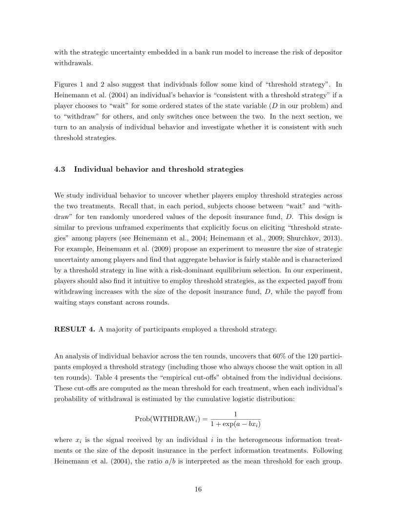
An analysis of individual behavior across the ten rounds, uncovers that 60% of the 120 partici-
pants employed a threshold strategy (including those who always choose the wait option in all
ten rounds). Table 4 presents the “empirical cut-offs” obtained from the individual decisions.
These cut-offs are computed as the mean threshold for each treatment, when each individual’s
probability of withdrawal is estimated by the cumulative logistic distribution:
Prob(WITHDRAWi) =1
1 + exp(a− bxi)
where xi is the signal received by an individual i in the heterogeneous information treat-
ments or the size of the deposit insurance in the perfect information treatments. Following
Heinemann et al. (2004), the ratio a/b is interpreted as the mean threshold for each group.
16
We compute these empirical thresholds for the two treatments and compare them with the
theoretical ones calculated in the previous section.
Table 4: Threshold behavior
Perfect information Heterogeneous information
% playing threshold strategy 70% 47.5%Theoretical cut-off
R=14 15.43 10.23R=16 25.45 20.23
Observed cut-offR=14 37.43 26.53R=16 26.65 30.62
In Table 4, we observe that the empirical thresholds are relatively higher than the theoretical
ones. This suggests that subjects are more prone to cooperate (play the wait strategy) than
predicted theoretically. This is in line with the observations in Heinemann et al. (2004), albeit
they do not observe such large differences. We also observe a higher propensity to employ
threshold strategies in the perfect information case.
4.4 Determinants of the probability of withdrawing
We show the robustness of our previous results by analyzing the determinants of the probability
of withdrawing. We perform a random effects panel probit model, where the dependent
variable is an indicator taking the value 1 if an individual withdraws and 0 otherwise. Our
key independent variables are D, the size of the deposit fund insurance and Info, a dummy
variable taking the value 0 for the perfect information treatments and 1 for the heterogeneous
ones.
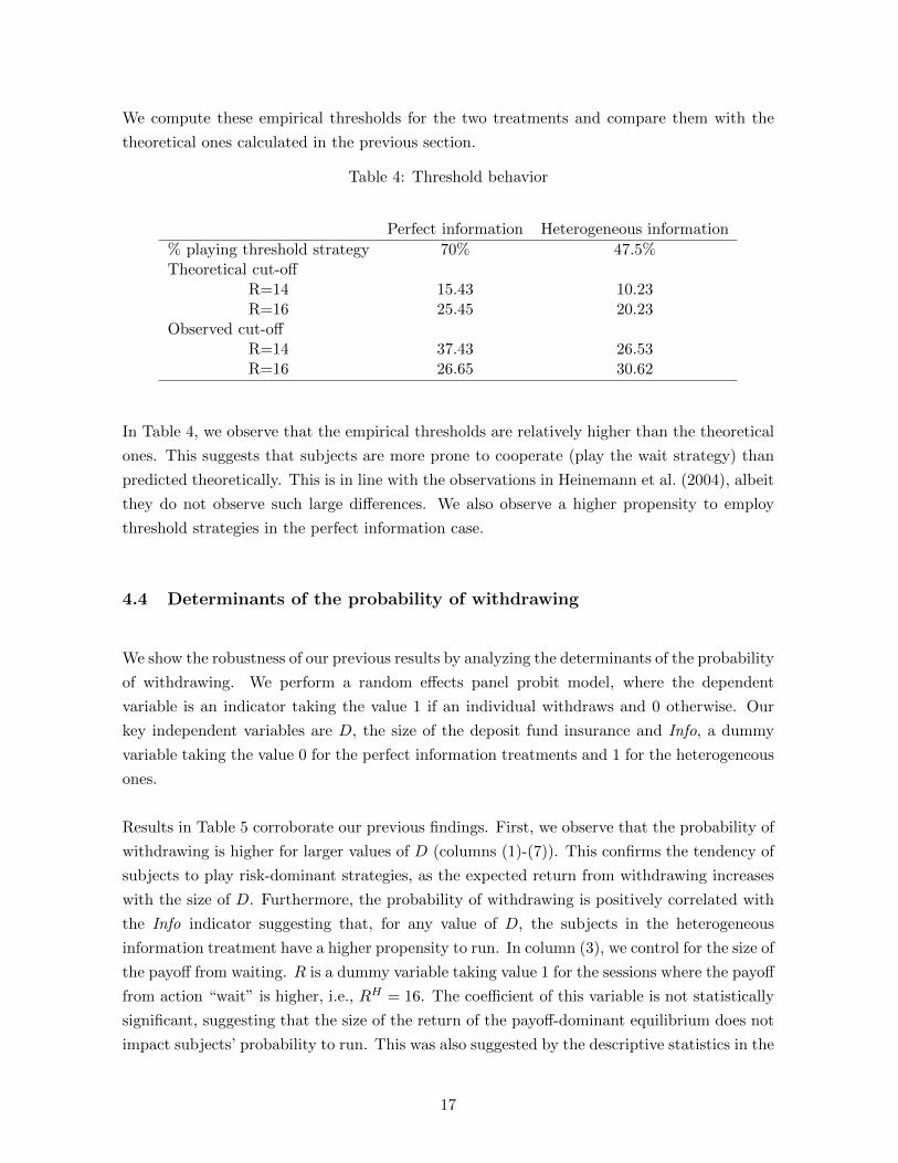
Results in Table 5 corroborate our previous findings. First, we observe that the probability of
withdrawing is higher for larger values of D (columns (1)-(7)). This confirms the tendency of
subjects to play risk-dominant strategies, as the expected return from withdrawing increases
with the size of D. Furthermore, the probability of withdrawing is positively correlated with
the Info indicator suggesting that, for any value of D, the subjects in the heterogeneous
information treatment have a higher propensity to run. In column (3), we control for the size of
the payoff from waiting. R is a dummy variable taking value 1 for the sessions where the payoff
from action “wait” is higher, i.e., RH = 16. The coefficient of this variable is not statistically
significant, suggesting that the size of the return of the payoff-dominant equilibrium does not
impact subjects’ probability to run. This was also suggested by the descriptive statistics in the
17
Table 5: Probability of withdrawing
(1) (2) (3) (4) (5) (6) (7) (8)D 0.036*** 0.037*** 0.037*** 0.038*** 0.039*** 0.037*** 0.037***
(0.0036) (0.0036) (0.0036) (0.0037) (0.0039) (0.0036) (0.0036)Info 0.636*** 0.637*** 0.656*** 0.721*** 0.620*** 0.215
(0.152) (0.152) (0.154) (0.155) (0.152) (0.205)R -0.0383
(0.159)Period -0.056***
(0.0158)Previous run 0.0921
(0.129)First round 0.203
(0.167)Guess Session 0.606***
(0.212)Hint 0.016**
(0.0071)Estimation 0.874***
(0.0873)
Observations 1,200 1,200 1,200 1,200 1,080 1,200 1,200 400Subjects 120 120 120 120 120 120 120 40
Panel probit regressions with random effects of the probability of withdrawing. D is the size of the depositinsurance fund in each round, Info is a dummy variable taking value 1 for the heterogeneous informationtreatments. R is a dummy variable taking value 1 for the sessions where the payoff from action “wait” ishigher, i.e., RH = 16. Period is a scalar for the rounds. Previous run is a dummy taking value 1 if a runtook place in the previous round. First round is a dummy for the first round. Guess session is a dummyfor the sessions which included an incentivized guess. Hint is the hint number received in the heterogeneousinformation treatments. Estimation is the estimated number of withdrawals stated by subjects in the guessrounds. Constant term included, but not reported. Standard errors in parentheses. *** denotes significanceat 1%, ** at 5% and * at 10% level respectively.
previous sections and is in line with previous experimental evidence on equilibrium selection
models (see, for example, Schmidt et al., 2003).
In column (4) we control for any learning effects by including a Period variable. The negative
and statistically significant coefficient suggests that subjects tend to coordinate on the payoff-
dominant equilibrium in later periods. Unreported results controlling for individual period
dummies show that the dummy variables for the last 3 periods are negative and statistically
significant. This is a common outcome in repeated coordination games. However, by contrast
to minimum effort games like Van Huyck, Battalio and Beil (1990; 1991), subjects do not
learn to coordinate on the inefficient equilibrium and coordination does not break down after
the occurrence of the Pareto inferior outcome. We also observe that a run occurring in the
previous period does not seem to affect behavior (column (5)), nor does the Period 1 outcome
(column (6)).14
14By contrast, Besancenot and Vranceanu (2014) study a repeated investment coordination game with apartner design and show that subjects are sensitive to past defaults, being more reluctant to invest after adefault, and more prone to invest prior to the first default.
18

In two of the heterogeneous information sessions we have also asked subjects to provide a guess
of the number of players they believe will withdraw in that period. This incentivized guess
seems to affect behavior and increases the propensity to withdraw (see column (7)). Finally, in
the heterogeneous information treatments, we can control for the signal that subjects receive.
This is captured by the Hint variable in column (8). In line with expectations, we find that
the signals are positively correlated with the propensity to withdraw. In this column, we also
control for participants’ actual estimation of the number of withdrawals in the rounds with
the incentivized guess. Results also show that subjects’ behavior is in line with their stated
beliefs, since their guess of the number of withdrawals (Estimation) is positively correlated
with the probability of withdrawal in column (8). This suggests that subjects withdraw for
higher levels of deposit insurance because they believe others will do so as well.
5 Conclusion
The Great Recession that followed the 2007-08 Global Financial crisis exposed the fiscal
fragility of many governments and a potential vulnerability of national deposit insurance
schemes to large common shocks. Despite the extensive deposit coverage in place in most
countries, a wave of bank runs that followed across Europe questioned the effectiveness of
these national insurance schemes in mitigating bank runs. As a consequence, in November
2015, the European Union established a European Deposit Insurance Scheme to strengthen
the protection of bank depositors across the Union. Yet this supranational fund can only cover
less than 1% of the total deposits of all banks in the EU.
In this paper, we study the effects of such deposit insurance schemes on the propensity to run
on a bank, whenever the size of the insurance fund may not suffice to cover all insured deposits.
We simulate bank depositors’ decisions in a typical coordination framework. However, contrary
to previous studies, in our experiment there is no “exogenous” trigger of bank runs (such
as forced withdrawals, contagion, informational cascades etc). We assume instead that the
deposit coverage is uncertain and may not cover the deposit in full. This uncertainty about
the actual level of coverage depends on (i) the size of the fund and (ii) the strategies of the
other players. At the same time, the return from waiting is common knowledge, and a payoff-
dominant equilibrium in which all depositors wait is always feasible. We analyze two main
contexts: (1) a perfect information setting in which depositors know the size of the deposit
insurance fund; and (2) a heterogeneous information treatment in which subjects only observe
an individual-specific, noisy signal about its size.
Our results show that uncertainty about deposit coverage leads to a significant breakdown
in coordination, the more so in the heterogeneous information treatment. Furthermore, we
19

observe that the higher the deposit insurance fund is, the higher the frequency of withdrawals.
This suggests that the coordination structure of the model “forces” players to adopt a risk-
dominant strategy, even when the risk and payoff-dominant strategies yield conflicting recom-
mendations. Moreover, in both treatments, a majority of players follow threshold strategies,
i.e., have a critical cutoff value of the actual/perceived deposit insurance fund around which
they switch between waiting and withdrawing.
Overall, our results cast doubt on the effectiveness of partial deposit insurance schemes to
increase the stability of the banking sector in a given country, in particular when depositors
fear a systemic banking crisis. The inability to cover all depositors can be “objective”, as
the result of an underfunded insurance scheme, or “perceived”, being related to low trust in
institutions. This low trust is probably higher in periods of political or economic turmoil,
making commitments of insuring the majority of bank deposits difficult to achieve (Ennis and
Keister, 2009). Our experiment highlights how this depositor uncertainty about the level of
deposit coverage can create a strong ex-ante propensity to run.
20
References
Arifovic, J., Hua Jiang, J. and Xu, Y. (2013), ‘Experimental evidence of bank runs as pure
coordination failures’, Journal of Economic Dynamics and Control 37(12), 2446–2465.
Besancenot, D. and Vranceanu, R. (2014), ‘Experimental evidence on the “insidious” illiquidity
risk’, Research in Economics 68(4), 315 – 323.
Brandts, J. and Cooper, D. J. (2006), ‘A change would do you good.... an experimental
study on how to overcome coordination failure in organizations’, The American Economic
Review pp. 669–693.
Brown, M., Trautmann, S. T. and Vlahu, R. (2016), ‘Understanding bank-run contagion’,
Management Science .
Carlsson, H. and Van Damme, E. (1993a), ‘Equilibrium selection in stag hunt games’, Frontiers
of game theory p. 237.
Carlsson, H. and Van Damme, E. (1993b), ‘Global games and equilibrium selection’, Econo-
metrica 61(5), 989–1018.
Chakravarty, S., Fonseca, M. A. and Kaplan, T. R. (2014), ‘An experiment on the causes of
bank run contagions’, European Economic Review 72, 39 – 51.
Cornand, C. and Heinemann, F. (2014), ‘Experiments on monetary policy and central bank-
ing’, Experiments in macroeconomics (Research in experimental economics, Volume 17)
pp. 167–227.
Demirguc-Kunt, A. and Detragiache, E. (2002), ‘Does deposit insurance increase banking sys-
tem stability? An empirical investigation’, Journal of monetary economics 49(7), 1373–
1406.
Demirguc-Kunt, Asli, E. K. and Laeven, L. (2013), ‘Deposit insurance database’, Policy Re-
search Working Paper 6934, Washington, DC: World Bank. .
Devetag, G. and Ortmann, A. (2007), ‘When and why? A critical survey on coordination
failure in the laboratory’, Experimental economics 10(3), 331–344.
Diamond, D. W. and Dybvig, P. H. (1983), ‘Bank runs, deposit insurance, and liquidity’,
Journal of Political Economy 91(3), 401–419.
Duffy, J. (2014), ‘Macroeconomics: a survey of laboratory research’, Working paper .
Dufwenberg, M. (2015), ‘Banking on experiments?’, Journal of Economic Studies 42(6), 943–
971.
21
Ennis, H. M. and Keister, T. (2009), ‘Bank runs and institutions: The perils of intervention’,
American Economic Review pp. 1588–1607.
Fischbacher, U. (2007), ‘z-tree: Zurich toolbox for ready-made economic experiments’, Exper-
imental Economics 10(2), 171–178.
Garratt, R. and Keister, T. (2009), ‘Bank runs as coordination failures: An experimental
study’, Journal of Economic Behavior & Organization 71(2), 300–317.
Georg, C.-P. (2013), ‘The effect of the interbank network structure on contagion and common
shocks’, Journal of Banking & Finance 37(7), 2216–2228.
Goldstein, I. (2010), ‘Fundamentals or panic: lessons from the empirical literature on financial
crises’, Available at SSRN 1698047 .
Goldstein, I. and Pauzner, A. (2005), ‘Demand-deposit contracts and the probability of bank
runs’, Journal of Finance 60(3), 1293–1327.
Harsanyi, J. C. and Selten, R. (1988), ‘A general theory of equilibrium selection in games’,
MIT Press Books 1.
Heinemann, F., Nagel, R. and Ockenfels, P. (2004), ‘The theory of global games on test: experi-
mental analysis of coordination games with public and private information’, Econometrica
72(5), 1583–1599.
Heinemann, F., Nagel, R. and Ockenfels, P. (2009), ‘Measuring strategic uncertainty in coor-
dination games’, The Review of Economic Studies 76(1), 181–221.
Hoggarth, G., Jackson, P. and Nier, E. (2005), ‘Banking crises and the design of safety nets’,
Journal of Banking & Finance 29(1), 143–159.
Kaufman, G. G. and Scott, K. E. (2003), ‘What is systemic risk, and do bank regulators retard
or contribute to it?’, The Independent Review 7(3), 371–391.
Kim, Y. (1996), ‘Equilibrium selection inn-person coordination games’, Games and Economic
Behavior 15(2), 203–227.
Kiss, H. J., Rodriguez-Lara, I. and Rosa-Garcıa, A. (2012), ‘On the effects of deposit insurance
and observability on bank runs: an experimental study’, Journal of Money, Credit and
Banking 44(8), 1651–1665.
Kiss, H. J., Rodriguez-Lara, I. and Rosa-Garcia, A. (2014), ‘Do women panic more than men?
an experimental study of financial decisions’, Journal of Behavioral and Experimental
Economics 52, 40–51.
Madies, P. (2006), ‘An experimental exploration of self-fulfilling banking panics: Their occur-
rence, persistence, and prevention’, The Journal of Business 79(4), 1831–1866.
22

Morris, S. and Shin, H. S. (1998), ‘Unique equilibrium in a model of self-fulfilling currency
attacks’, American Economic Review 88(3), 587–597.
Morris, S. and Shin, H. S. (2001), Rethinking multiple equilibria in macroeconomic modeling,
in ‘NBER Macroeconomics Annual 2000, Volume 15’, MIT PRess, pp. 139–182.
Morris, S. and Shin, H. S. (2003), ‘Global games: theory and applications’, Econometric
Society Monographs 35, 56–114.
Schmidt, D., Shupp, R., Walker, J. M. and Ostrom, E. (2003), ‘Playing safe in coordination
games:: the roles of risk dominance, payoff dominance, and history of play’, Games and
Economic Behavior 42(2), 281–299.
Schotter, A. and Yorulmazer, T. (2009), ‘On the dynamics and severity of bank runs: An
experimental study’, Journal of Financial Intermediation 18(2), 217–241.
Shurchkov, O. (2013), ‘Coordination and learning in dynamic global games: experimental
evidence’, Experimental Economics 16(3), 313–334.
Stahl, D. O. and Wilson, P. W. (1994), ‘Experimental evidence on players’ models of other
players’, Journal of economic behavior & organization 25(3), 309–327.
Van Huyck, J. B., Battalio, R. C. and Beil, R. O. (1990), ‘Tacit coordination games, strategic
uncertainty, and coordination failure’, The American Economic Review 80(1), 234–248.
23

A Instructions - Heterogeneous information treatments
Thank you for participating in this economic experiment, in which you will be given the
opportunity to earn money. We ask you not to communicate with each other from now on and
turn off all mobile phones. If you have any questions, please raise your hand, and the instructor
will come to you. The instructions below will explain to you the decisions you have to make
throughout the experiment. Your identity will not be revealed to the other participants.
The experiment has 10 rounds. At the end of the experiment, one round will be randomly
picked by the computer and you will receive the payoffs from that round.
At the beginning of each round you receive 10 Euro, which are deposited in a bank. A bank
is formed of 5 depositors. Note that the depositors at a bank will change in each round, so
the likelihood you will play with all the same people in future rounds is very low.
The bank will invest the money you and the other 4 depositors have placed with it in a project
that will provide a known return. You have to decide whether to keep your money in the bank
(WAIT) or withdraw your deposit (WITHDRAW).
Your payoff depends on your decision, but also on what the other players decide to do.
• If you WAIT, your payoff will decrease the more depositors at your bank withdraw as
shown in the table below.
• If you WITHDRAW, you get back your deposit of 10 Euro if less than 3 people (including
yourself) decide to withdraw.
Table 6: Promised returns
Number of depositors who withdraw Payoff if you withdraw Payoff if you wait
0 - 16 e1 10 e 15 e2 10 e 14 e3 minimum{D/3, 10} e 04 minimum{D/4, 10} e 05 minimum{D/5, 10} e 0
24
Deposit insurance
If 3 or more depositors at your bank decide to withdraw, the bank will fail and lose all its
investment. How much you can recover from your deposit will then depend on a “deposit
insurance fund”. This fund has an endowment, called D, which is unknown to all partic-
ipants and is drawn randomly from the interval [0, 50]. All numbers in the interval [0, 50]
have the same probability to be drawn. This number is the same for everyone. When you
make your decision to withdraw or wait you will not know the chosen number D. You will
however receive a hint about the drawn number D and this hint will be selected from the
interval [D-10, D+10]. Each participant will received his own hint number. On the basis of
this hint you can decide whether to withdraw or not. If 3 or more depositors withdraw and
the bank fails, depositors who withdraw get either the initial deposit of 10 Euro or an equal
share of D, when D is not big enough to cover all depositors who withdraw. However, if the
bank fails and you wait, you get nothing.
For example, the unknown number D drawn by the computer is 15. The 5 participants will
receive hints from the interval [5, 25] such as 6, 24, 9, 13, 22. The participant who receives
hint 6 knows that D must be between 0 and 16. The participant who receives hint 24 knows
that D must be between 14 and 34 etc. If 4 depositors withdraw, then they will each receive
D/4=3.75 Euro, while those who wait receive 0.
Remember, you do not know the true value of D, you just receive a hit number which is an
approximation of D. You also don’t know the number of people who decide to withdraw.
Therefore, you cannot exactly determine your payoffs in case the bank fails.
In each round you will see 2 screens. In the first screen, you will need to decide if withdrawing
your deposit or leaving the money in the bank. You will also be asked to give your guess
about the number of people you think will withdraw given the information received in that
round. If your guess is correct, you will get an additional payoff according to the formula
5+5/(error+1), thus the smaller the error (the closest your guess) the higher the payoff you
can receive (if your guess is perfect you get 10 Euro). In the second screen you will see:
1. the actual number D
2. your decision
3. how many participants have withdrawn
4. your gain from the bank game in that round
25