experimental dynamic behavior of free standing multi-block

1

Journal of Earthquake Engineering © A. S. Elnashai and N. N. Ambraseys

EXPERIMENTAL DYNAMIC BEHAVIOR OF FREE STANDING MULT I-BLOCK STRUCTURES UNDER SEISMIC LOADINGS

FERNANDO PEÑA* Instituto de Ingeniería, UNAM

Circuito Escolar, Ciudad Universitaria, 04510 Mexico city, Mexico

PAULO B. LOURENÇO University of Minho, ISISE, Department of Civil Engineering

Azurem, 4800-058 Guimarães, Portugal

ALFREDO CAMPOS-COSTA Laboratório Nacional de Engenharia Civil, Av. Brasil 101

1700-066, Lisboa, Portugal

Received (received date) Revised (revised date)

Accepted (accepted date)

This paper describes the dynamical behavior of free standing block structures under seismic loading. A comprehensive experimental investigation has been carried out to study the rocking response of four single blocks of different geometry and associations of two and three blocks. The blocks, which are large stones of high strength blue granite, were subjected to free vibration, and harmonic and random motions of the base. In total, 379 tests on a shaking table were carried out in order to address the issues of repeatability of the results and stability of the rocking motion response. Significant understanding of the rocking motion mechanism is possible from the high quality experimental data. Extensive experimental measurements allowed to discuss the impulsive forces acting in the blocks and the three-dimensional effects presented in the response.

Keywords: rocking motion, rigid bodies, multi-block structures, earthquakes, dynamics.

1. Introduction

Free standing blocks are objects particularly vulnerable to lateral seismic loading, since they have no tensile strength and stability is ensured if the resultant force from all actions falls inside the base of the block. The study based upon the assumption of continuum structures is not realistic and models based on rigid-block assemblies provide a suitable framework for the study of dynamic response under seismic actions. In this context, the problem is primarily concerned with Rocking Motion (RM) dynamics (Augusti and Sinopoli, 1992).

Rocking motion is defined as the oscillation of the rigid bodies (RB) present in a structure when the center of rotation instantly change from one reference point to another.

*Correspondence to: Fernando Peña, e-mail: [email protected]

2 F. Peña, P.B. Lourenço and A. Campos-Costa

This instantaneous change produces a loss of energy due to an impulsive force (Prieto et al. 2004) and it has been shown that it is not possible to study a structure that presents RM as an oscillator of one degree of freedom (Makris and Konstantinidis, 2003).

Studies on RM have been carried out for a long time. The first studies are from the late the 19th century (Milne, 1881; Perry, 1881). However, Housner's work (1963) is considered as the first systematic study about the dynamics of RB and is known as the classical theory. Housner (1963) obtained the equation for the period of the system, which depends on the amplitude of rocking, and the equation for the restitution coefficient. This author also proposed expressions to calculate the minimum acceleration required to overturn a single RB. The principal hypotheses of Housner are: • the block and its base are perfectly rigid, • the surface of the base is horizontal, • the block is symmetric with respect to the vertical central axis, • there is no sliding of the RB, • only in-plane (2D) motion is considered, • the impact of the block during rocking is not elastic, meaning that the block does not

jump. Therefore, at least one contact point always exists between the RB and its base,

• angular moment conservation exists (before and after impact), • three parameters, detailed below, govern the differential equation of RM.

With these hypotheses, the parameters obtained by Housner (or theoretical

parameters) depend only on the block geometry and mass, and not specifically on the material of the block or the base. Also, rocking motion is the only possible motion that a RB can experiment.

After Housner (1963), several studies have been made (Ishiyama, 1982; Lipscombe, 1990; Makris and Roussos, 1998; Pompei et al., 1998; Psycharis, 1982; Winkler et al., 1995; Yim et al., 1980; Zhang and Makris 2001) on the RB under different conditions. The following conclusions can be drawn from these studies: • the theoretical parameters are different from the parameters obtained from laboratory

tests, • the friction between the base and the block is not infinite, thus it is possible to have

slide behavior, • the motion of a RB is a combination of rocking, sliding and jumping. In fact, there

are six motion states (Ishiyama, 1982): a) rest, b) slide, c) rotation, d) slide–rotation, e) translation–jump, and f) rotation–jump,

• the response of a RB is very sensitive to the boundary conditions, the impact (coefficient of restitution) and the type of the base motion, e.g. harmonic or random, frequency contents, etc. Despite the significant past researches the study of multi-block systems remains a

challenging task. The main reasons are the need to propose adequate criteria for the

Dynamical behavior of free standing blocks under seismic loadings

3

seismic evaluation and the lack of comprehensive experimental data. It is stressed that comprehensive numerical and analytical studies on RM exist, but there are few authors describing only the experimental nature of RB under RM.

In this context, the objective here is to draw new conclusions about RM exclusively from high quality and fully reported experimental data. An extensive experimental investigation on the rocking response has been carried out at the shaking table of the National Laboratory of Civil Engineering (LNEC) of Portugal using blue granite stones. Large single blocks of different geometries subjected to different types of base motion, as well as multi-block structures, have been considered. The multi-block structures include two stacked blocks (referred to as stacked blocks or bi-block structure) and a three-block portico (referred as trilith). Particular attention was given to the experimental data acquisition, repeatability of the results and stability of the RB. The numerical simulation of the experimental research on single blocks can be found in Peña et al. (2007).

2. Details of the Testing Program

2.1. Characteristics of the Specimens

Three types of free standing multiblocks structures were tested (Fig. 1): a) four single blocks of different geometries, b) an ensemble of two stacked blocks, and c) a three-block portico. In order to minimize damage during testing, blue granite stone was selected as material; since it is a very hard stone. The mechanical properties of the granite are given in Table 1 (Transgranitos, 2007).

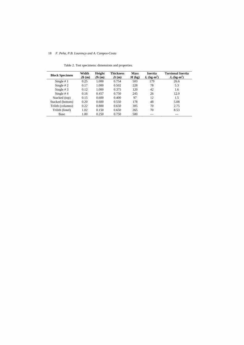
Each stone has different geometrical dimensions (Table 2). The dimensions of the single specimens 1, 2 and 3 were fixed to achieve a Height-Width ratio (h/b) of 4, 6 and 8, respectively, being the height of the three specimens equal to 1 m. In addition, the fourth single specimen was designed with a non-rectangular geometry in order to compare its performance with the rest of the stones. For this reason, the specimen 4 presents a large 45 degree cut (40 mm) at the base (Fig. 1a)

The Height-Width ratio of the stacked blocks is 3 and 4, for the top and bottom blocks, respectively; while the columns of the trilith have an h/b ratio of 4 (Fig. 1b,c).

In order to minimize the three-dimensional (3D) effects, all the blocks were designed with a Thickness-Width ratio (t/b) of 3. On the other hand, with the aim of reducing the continuous degradation at the block corners occurring at every impact, the stones were manufactured with a small cut of 5 mm oriented at 45 degrees at their bases. After sawing the specimens, no additional treatment of the base was carried out.

A foundation of the same material was used as the base where the blocks are free to rock. This foundation was rigidly fixed to the shaking table by means of four steel bolts.

4 F. Peña, P.B. Lourenço and A. Campos-Costa 2.2. Test Setup

The uniaxial shaking table of LNEC has a payload of 6 tons, a maximum displacement of ±10 mm and a maximum acceleration of 4.5g with an input frequency of 20 Hz. These values are adequate for the type of experiments performed.

The data acquisition system was designed to describe the position of the specimens at each instant of the tests and, simultaneously, to avoid the possibility that the system influences the response of the specimens. In this context, the data acquisition is based on monitoring Light Emission Diode Systems (LEDS) by means of high resolution cameras. The Position Sensor is a light spot detector able to measure two-dimensional movements. A photodiode sensor, namely a semiconductor position-sensitive detector (PSD) was used as the light receiving element. A LED target is connected to the object to be measured and the position is measured optically. This eliminates noise errors and enables accurate position measurement. The position resolution obtained is of 1/5000. The measurement values are obtained as serial output to the data acquisition system through National Instruments devices and associated software.

The main data obtained with the above system were rotations around Y and Z axes, and linear displacements X and Y. The system coordinate is depicted in Figure 2a. Rotations Y and Z were directly measured by means of a mirror linked to the blocks surface on the West face of the specimens. The LED was located at the same position of the measuring camera and the light ray emitted is reflected at the mirror, so that a larger measured range is obtained (±100 mm). Details of the mirror system data acquisition are shown in Figure 2b,c. Displacements X and Y were measured in two points of the North face of each specimen through the LEDs coordinates directly (Figure 2a,d).

In addition to the LED-Camera system, two accelerometers were placed at the top of each single specimen. One triaxial accelerometer was located in the North face and one biaxial accelerometer was located in the South face. The displacements and accelerations of the shaking table were also measured.

Two safety frames were placed at each side (East and West) of the specimen in order to protect the table and the stones in case of overturning. In addition, the top block of the bi-block structure and the lintel of the trilith were held by safety cables in order to avoid a possible downfall. It is noted that the cables had enough length to allow free rocking and sliding of the blocks (Figure 2).

It is noted that in pure Rocking Motion, the system has only one degree of freedom (DOF) but monitoring of extra degrees of freedom provides a way to measure possible out-of-plane and sliding motions.

2.3. Types of Base Motion

Three different types of motion were considered: a) Free rocking motion, b) Harmonic motion, and c) Random motion. The first type of test allows to identify the parameters used in the classical theory and at the same time to calibrate analytical models (Peña et al., 2007).


5

The harmonic tests allow to study the dynamic behavior of single blocks undergoing RM regime subjected to a slowly varying forced vibration. Three different types of harmonic motion were used: a) constant sine, b) frequency sweep test (run-down and run-up) with constant amplitude, c) sine with constant frequency and amplitude modulated with a Hanning function (Hanning sine).

The behavior of the RB under earthquake conditions was studied with a random test. Thirty synthetic earthquakes compatible with the design spectrum proposed by Eurocode 8 (2004) were generated. In order to identify them, the accelerograms were named consecutively with the number of generation. The constant branch of the spectrum is located between 0.1 and 0.3 seconds, with a spectral acceleration of 7 m/s2 while the peak ground acceleration is 2.8 m/s2. The main aim of the study is to address stability of RM under random motion.

In total 379 tests were carried out in the shaking table using the three different inputs: a) 175 for the single blocks; b) 82 for the stacked blocks; and c) 22 for the trilith.

2.4. Sliding Motion

The specimens and the loads were designed in order to avoid sliding motion of the blocks, since the aim of the research was to study pure rocking motion behavior. In this context, sliding will occur when the following conditions are fulfilled (Shenton, 1996):

h

ba sgs << ηη ; . (2.1)

where ηs is the static coefficient of friction and ag is the peak ground acceleration as fraction of the gravity acceleration.

The static coefficient of friction for the specimens is 0.577 (Table 1). The ratio b/h is equal to 0.250, 0.170 and 0.125 for specimens 1 to 3 respectively and 0.250, 0.333 and 0.275 for the stacked blocks (top and bottom) and columns of the trilith respectively. Thus, the second condition is not fulfilled, and no-sliding should occur. Specimen 4 has a ratio b/h equal to 1.3, but the maximum ground acceleration was 0.28 for random motion and 0.2 for harmonic motion. Thus the first condition is not fulfilled and no-sliding should occur.

3. Parameters of the Classical Formulation

The differential equation of RM of a rectangular RB, with base 2b and a height 2h, is (Housner, 1963):

g

tapp

)()cos()sin( 22 θαθαθ mm =±′′ . (3.1)

where θ is the rocking angle, (’ ) means differentiation with respect to time t, g is the acceleration of gravity and the ± sign refers to the domains of the rocking angle θ>0 and θ<0 respectively, α is the critical angle and p is a geometrical parameter and a(t) is the base motion acceleration.


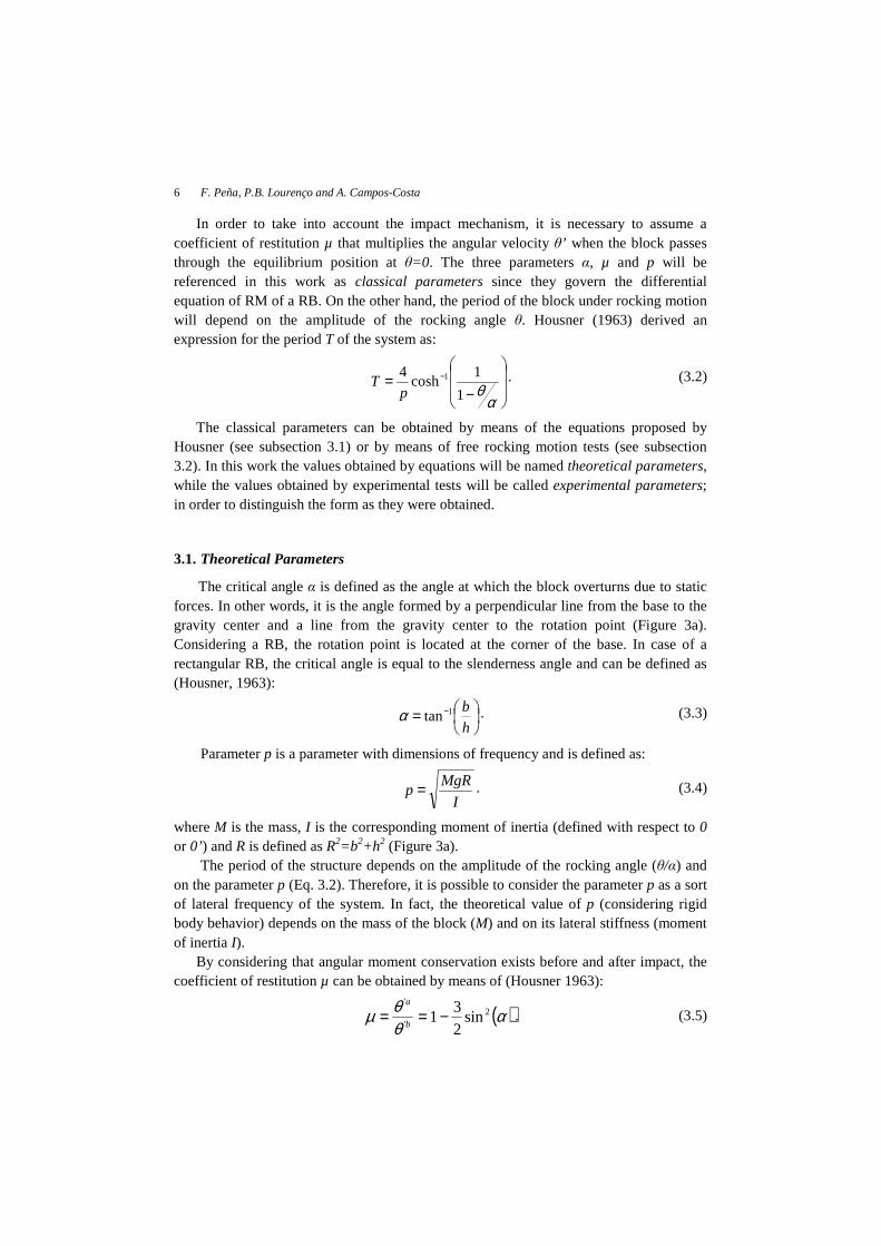
In order to take into account the impact mechanism, it is necessary to assume a coefficient of restitution µ that multiplies the angular velocity θ’ when the block passes through the equilibrium position at θ=0. The three parameters α, µ and p will be referenced in this work as classical parameters since they govern the differential equation of RM of a RB. On the other hand, the period of the block under rocking motion will depend on the amplitude of the rocking angle θ. Housner (1963) derived an expression for the period T of the system as:

−= −

αθ1

1cosh

4 1

pT . (3.2)

The classical parameters can be obtained by means of the equations proposed by Housner (see subsection 3.1) or by means of free rocking motion tests (see subsection 3.2). In this work the values obtained by equations will be named theoretical parameters, while the values obtained by experimental tests will be called experimental parameters; in order to distinguish the form as they were obtained.

3.1. Theoretical Parameters

The critical angle α is defined as the angle at which the block overturns due to static forces. In other words, it is the angle formed by a perpendicular line from the base to the gravity center and a line from the gravity center to the rotation point (Figure 3a). Considering a RB, the rotation point is located at the corner of the base. In case of a rectangular RB, the critical angle is equal to the slenderness angle and can be defined as (Housner, 1963):

= −

h

b1tanα . (3.3)

Parameter p is a parameter with dimensions of frequency and is defined as:

I

MgRp = . (3.4)

where M is the mass, I is the corresponding moment of inertia (defined with respect to 0 or 0’) and R is defined as R2=b2+h2 (Figure 3a).

The period of the structure depends on the amplitude of the rocking angle (θ/α) and on the parameter p (Eq. 3.2). Therefore, it is possible to consider the parameter p as a sort of lateral frequency of the system. In fact, the theoretical value of p (considering rigid body behavior) depends on the mass of the block (M) and on its lateral stiffness (moment of inertia I).

By considering that angular moment conservation exists before and after impact, the coefficient of restitution µ can be obtained by means of (Housner 1963):

( )αθθµ 2

'

'

sin2

31−==

b

a

. (3.5)


7

where θ’ a and θ’ b are the angular velocities just after and before the impact, respectively. The values of the classical parameters obtained via equations (3.3) to (3.5) will be

referenced in this work as theoretical parameters.

3.2. Experimental Parameters

The experimental parameters can be obtained from free rocking motion tests by mean of a minimized error surface (Tso and Wong, 1989). Since for free RM, the energy is conserved between two consecutive impacts, it is possible to derive an analytical expression for the time t of the maximum amplitudes of rocking angle before and after impact n, given by:

∫ − −−=

0

1 )cos()cos(2

1nt

nx

dx

pt

αα. (3.6)

Equation (3.6) allows to find the experimental values, here denoted with an *, for the time at each impact tn

* and the rocking angle amplitude rn* after the nth impact.

Parameters α and p are obtained by minimizing the error surface:

∑∑ −=n nn ttp 2* )(),(α . (3.7)

On the other hand, taking into account that the relation between energy after the nth impact En and the initial energy E0 is given by En=E0µ

2n, the coefficient of restitution for each impact µn can be obtained, using the fitted value of α and the experimental amplitudes rn

*, by:

n

nn r

r 2

1

*0

*

)cos()cos(

)cos()cos(

−−−−

=ααααµ . (3.8)

The final value of µ is obtained by averaging the recorded values of µn in the different impacts.

3.3. Theoretical vs. Experimental Parameters

The aim of the minimization process adopted here is to overcome the difficulties to extract the value of the classical parameters. The experimental parameters may not match with the theoretical ones due to: • Detailed measurements in the real dimensions of the blocks. Small variations in the

geometry give differences in the classical parameters, as in specimens 1 and 2. • Real position of the gravity center. In the case of non-homogeneous material or an

arbitrary shape of the block, as in specimen 4. • Rotation surface. When the block is completely rigid, the rotation point is located at

the corner of the base. But when the block is not completely rigid, the rotation point does not exist. In this case, the block will tend to rotate on a finite surface (Figure 3a). The size of this surface will depend on the material stiffness. It will tend to zero (single point) when the stiffness of the material tends to infinite.


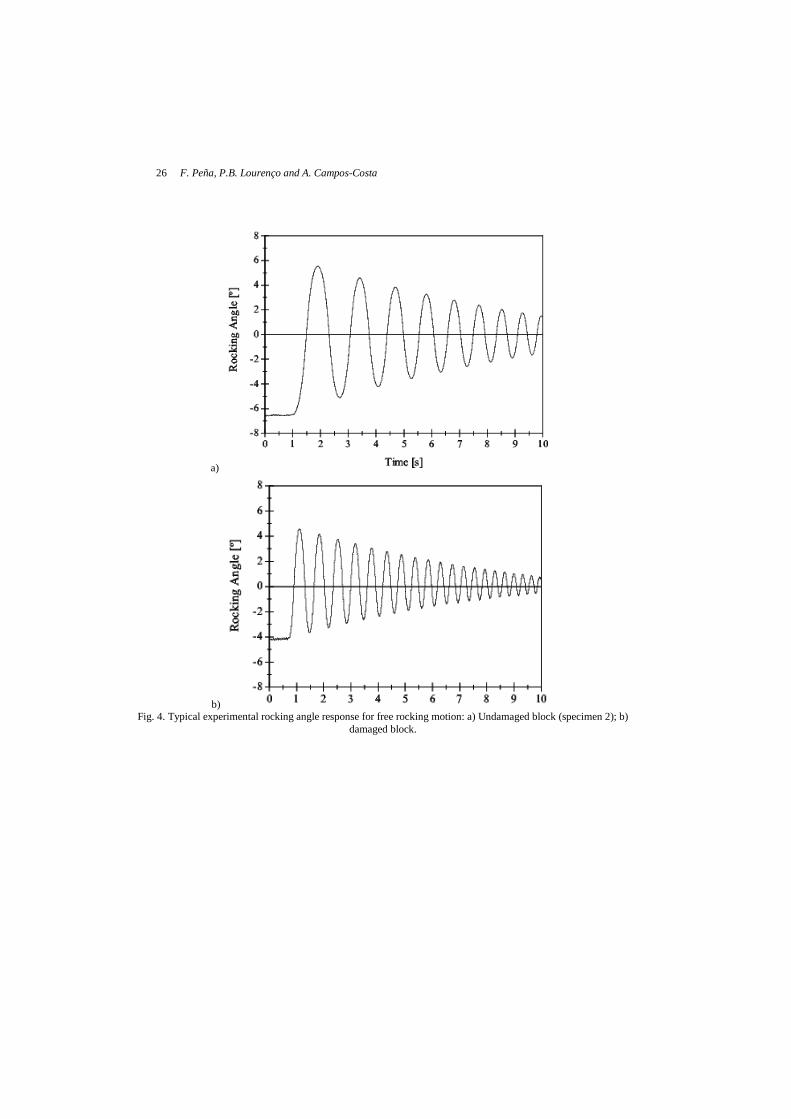
• Damage. Even minor damage at the base of the block changes the values of the classical parameters (Figure 3b). As an example, Figure 4a shows a typical free rocking motion of an undamaged block, with the amplitude of the rocking angle decreasing at each impact. Figure 4b shows a typical free rocking motion of a block that was damaged on one side of the basea, as shown schematically in Figure 3b. In this case, the amplitude of the rocking angle is different depending on sign of movement, yielding non-symmetric response. In the example, the maximum rocking angle in each cycle is always half degree greater in the damaged side, when compared to the undamaged side. As a consequence, the block has two different values of α depending on the side of rocking.

• Three dimensional effects, as in specimen 3 (addressed below). Table 3 shows the theoretical and experimental values of the classical parameters, for

the single blocks and for the two blocks of the stacked structure. It is worth to note that the blocks of the stacked structure were tested in free rocking as single blocks first and as stacked blocks second. Free rocking tests were not carried out for the trilith due to the complexity of forcing the whole structure to have the same initial rotation angle.

Experimental parameters for specimens 1, 2 and the top block of the stacked structure are similar to the theoretical values, with differences up to 6% for α. Specimen 4 and bottom block present moderate differences in their parameters, especially for α, with errors lower than 14%. Specimen 3 is a particular case with three-dimensional effects addressed later in the paper.

The differences in the α values are generally related with the small 45 degree cuts of 5 mm in the base, which provides a lower experimental value. The coefficient of restitution µ is related to damping of the system. The experimental values are slightly higher than the theoretical values because there is not conservation of angular moment, since the bodies are not fully rigid. On the other hand, p presents a random variation with respect to the theoretical values. These differences are due to the microscopical roughness of the contact surfaces, as well as to the fact that blocks and base are not fully rigid.

4. Dynamics of Free Rocking Motion

Typical acceleration, velocity and displacement values on the N-E top corner of the single blocks are depicted in Figure 5. Velocity and displacements were obtained by numerical integration of the acceleration. The horizontal acceleration is practically constant and only changes its sign instantly at each impact, the velocity is linear and changes its sign at each impact, while displacement is parabolic and decreases with the number of impacts. The velocity is zero with the maximum displacement and vice-versa. It is interesting that the horizontal acceleration remains constant even in the last cycles of rocking; while the velocity and the displacements tend to zero. Thus, the amplitude of

a The damaged block is not one of the four specimens used during the experimental test. This block was a fifth

block damaged due to incorrect handling before testing. Only one free rocking test was performed on this block and it was not considered as part of the specimens tested.


9

these two quantities is related to the time between impacts, called semi–period. On the other hand, the vertical acceleration is almost zero during each semi–period, becoming impulsive during the impact.

In order to understand the dynamics of the free rocking motion, one cycle, here shown between maximum displacements in a given direction, is detailed in terms of acceleration (measured at the top of the block) and rocking angle, as shown in Figure 6. When the free cycle begins with an initial angle different than zero, the E-W acceleration is different than zero, while the N-S (out-of-plane) acceleration is zero. The accelerations remain almost constant until the impact occurs. In this moment an impulsive acceleration (force) appears in the three directions. Due to the impulsive acceleration a variation of the acceleration (vibration) appear after the impact. The E-W acceleration changes sign and will tend to remain constant with the same value of the initial acceleration. The N-S and Vertical accelerations will tend to zero. For this particular case, the maximum impulsive accelerations in E-W and Vertical directions are in the same order of magnitude, while in the N-S direction the maximum value is around the half. This impulsive out-of-plane acceleration causes 3D effects in the RB, as shown later. For one cycle, the vertical acceleration has a shape of a Dirac–δ, while the N-S acceleration shape is a semi–Dirac–δ. The E-W acceleration presents the typical Z shape of rocking systems.

Figure 7a shows a typical free rocking motion of the stacked blocks, where the bottom block moves to the rest position and the top block increases the rotating angle. As soon as the bottom block movement is stopped, the top block continues rocking as in free vibration of a single block.

Figure 7b shows the horizontal acceleration measured at the top of each block, while Figure 7c shows the rocking angle vs. horizontal acceleration. It is observed that the behavior of both blocks is not similar to the behavior of a single block, since the response of the blocks is affected by the movement of the other block. In this case, the horizontal acceleration of the bottom block is not constant at each semi-period, and at the end of the motion the acceleration decreases gradually to zero.

5. Rocking Due to Harmonic Motion

5.1. Single Blocks

The response of a RB under harmonic motion depends on the frequency and the amplitude of the harmonic motion. To illustrate this fact, Table 4 shows typical frequencies and amplitudes at which a single block shows rocking. A clear relationship between the harmonic motion and the rocking motion exists. It is clear that if the amplitude increases while the frequency remains constant, the amplitude of the rocking increases too. On the other hand, and in general, if the frequency of the motion increases, while the amplitude remains constant, the rocking angle decreases. Thus, there are some couples of frequencies and amplitudes of harmonic motion for which the RB will experience rocking. The set of these couples is called rocking motion space.


The rocking motion of a RB under harmonic loads shows three states of movement (Figure 8a,b). At the beginning of loading, a transient response is found. After this state, the RB moves with the frequency of the load in a stationary response. Finally, free rocking motion appears upon termination of the loading.

In the case of frequency sweep tests (run-down and run-up), the three states of the rocking motion are found too. Figures 8c,d shows a run-down test from 5.0 to 0.5 Hz and 3 mm of amplitude and a run-up test from 0.5 to 5.0 Hz and 6 mm for specimen 2. Since in a frequency sweep test, the load moves inside or outside of the rocking motion space, the response of the RB is rather different than the constant sine. For both frequency sweep test, the first move of the RB is similar to a constant sine test. Thus, the amplitude of the first rocking angle will depend on the frequency and the amplitude of the load. For the case illustrated, the rocking motion, for the run-up test, begins after 15 seconds. This means that the frequencies below 2 Hz do not produce rocking motion with 6 mm of amplitude. On the other hand, for the run-down test, the RB begins to rock immediately with the first couple of frequency (5 Hz) and amplitude (3 mm).

The run-down test is in general more dangerous than the run-up test. In the run-down case, as the frequency becomes lower, the amplitude of the rocking motions grows up (see Table 4). This effect is amplified because the frequency of the system changes with the rocking angle and becomes similar to the frequency of the load. On the other hand, in the run-up test the opposite phenomenon was found. As the frequency becomes higher, the amplitude of the rocking motions decreases and, at the same time, the frequency of the system moves apart from the frequency of the load.

5.2. Stacked Blocks

Figure 9 shows the four possible patterns of rocking motion that the stacked blocks may exhibit (Spanos et al., 2001), which can be divided in two main groups. The first group (patterns 1 and 2) corresponds to a two degree of freedom system response, in which the two blocks rotate in the same or opposite direction. The second group (patterns 3 and 4) corresponds to a single degree of freedom system response. In particular, pattern 3 is equivalent to a single rigid structure, while pattern 4 is the case where only the top block experiences rotation.

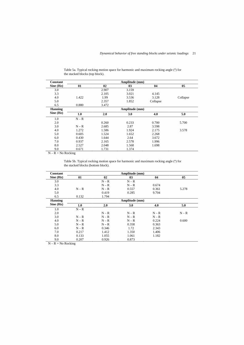
The main patterns found in the stacked blocks tests were patterns 2 and 4. These patterns are associated with the amplitude and frequency of the loads. Pattern 2 was recorded with constant sine base motion with frequencies between 4 and 5 Hz and amplitudes greater than 4 mm, with frequency of 6 Hz and amplitudes greater than 3 mm and frequency 7 Hz with amplitudes greater than 1 mm. Pattern 4 was recorded with constant sine base motions with frequencies between 1 and 5 Hz with amplitudes lesser than 4 mm. Therefore, it is possible to construct the rocking motion space for stacked blocks as shown in Table 5. However, there is not clear relationship between the frequency and amplitude with the maximum rocking angle, as found in the single blocks.


11

5.3. Trilith

Figure 10 shows schematically the final displacement patterns that the trilith exhibited during the constant sine base motion. Each pattern was associated to a particular frequency and amplitude couple, even if it is likely that the response is chaotic in this particular case. It can be seen that a highly three dimensional behavior is presented, especially for higher frequencies. In general, it is possible to classify the different patterns in two main groups. The first one correspond to a lateral motion of the entire structure with sliding of the pillars (Figures 10b,c,d), that it corresponds to a range of frequencies between 1 to 3.3 Hz. The second group corresponds to torsional motion of the lintel with sliding of the pillars (Figures 10e,f).

Here, it is necessary to bear in mind that the multiblock structures are not continuous structures and relative displacements between elements can occur. This relative movement between elements modifies the stability of the construction even with small relative displacements because the elements loose the perfect contact among them. The lack of contact can be considered similar to damage in the base that decreases the critical angle α; becoming the structure more vulnerable to lateral forces (see subsection 3.3).

A typical behavior of the trilith under constant sine motion (3.3 Hz and 5 mm of amplitude) is depicted in Figure 11. The lateral displacements of the pillars (Figure 11a) show the presence of rotational sliding between them, while the lateral displacement of the lintel (Figure 11b) shows the lateral sliding that the lintel suffers during the harmonic motion. The rocking angle behavior of the pillars is similar to the rocking angle of the single blocks under harmonic motion, with transient state at the beginning of the motion, stationary state during the loading and the free rocking motion at the end of loading. However, it is worth to note that the amplitude of the rocking angle during the stationary state is not symmetric for each pillars (Figures 11c,d). For this particular case, the amplitude for one sign of movement is around 1 degree, while for the other is around 0.75 (25% lower). This is due to the sliding rotation of the pillars and the sliding of the lintel that modify the contact among elements and do not allow pillars to rock completely free. In fact, the rocking angle of the lintel shows a residual rocking angle in one direction due to the natural difference in geometry of the stone blocks (Figure 11e). Finally, Figure 11f shows the difference of the rocking angle between pillars, which allows to understand if the pillars rock in phase. The very small values found indicate that the pillars rock in phase, while the residual value of 0.25 degrees is in agreement with the difference in amplitude for each side of the rocking angle of the pillars (Figures 11c,d).

6. Repeatability Test

6.1. Single Blocks

Several tests were repeated in order to study the repeatability of the response of the RB under forced excitation. For the case of harmonic motion the tests selected for repetition were: a) specimen 1 with the Hanning sine of 3.3 Hz / 7 mm; b) specimen 2


with constant sine of 3.3 Hz / 6 mm; c) specimens 3 and 4 with all the constant sine tests. All these tests show that the repeatability in the harmonic motion exists. The six tests performed with specimen 1 subjected to Hanning sine of 3.3 Hz / 7 mm are depicted in Figure 12a. The responses of all six tests are similar. Taking the first test as reference, the differences (in percentage) of the values of the maximum rocking angle is below 3% except for test number 5 that presents an error of 10%. Figure 12b shows the Fourier spectra of the rocking angle. It can see that all six spectra are practically the same and they show little differences on frequencies up to 10 Hz. The Fourier spectra show two peaks. One is related with the load frequency (3.3 Hz), while the other (1.9 Hz) is associated to the transient response.

In the case of random motion, the tests were carried out with the generated random motion, under increasing load factors that scale the original accelerogram. Each test was repeated at least two times. Typical responses are shown in Figures 12c,d in terms of rocking angle curves for specimen 2 loaded with earthquake 20 and load factors of 1.1 and 1.3. With a load factor of 1.1, the specimen has a maximum rocking angle of 6.8º for one test while overturning in the other test. It is worth noticing that during the first six seconds the behavior of the RB is similar for the two tests. With the load factor of 1.3, did not overturn for any test and both behaviors are similar during the first seconds. However, at the end of the load (at 16.2 s) the behaviors became rather different, especially during the free rocking motion.

6.2. Stacked Blocks

Five tests were repeated twice in order to check the repeatability of the tests under harmonic motion. The tests repeated were: a) constant sine of 3 Hz / 3 mm; b) constant sine of 5 Hz / 2 mm; c) Hanning sine of 5 Hz / 4 mm; d) Hanning sine of 6 Hz / 4 mm; and e) Hanning sine of 7 Hz / 3 mm.

The tests with constant sine of 3 Hz / 3 mm and the Hanning sine of 7 Hz / 3 mm were the only two tests that showed repeatability (Figure 13a,b). The other three tests showed rather different behavior of the blocks (Figure 13c).

Figure 13a shows the rocking angle measured in the blocks for the repeatability test with constant sine of 3 Hz / 3 mm. In this case, both responses are practically the same, as shown in the Fourier spectra of the rocking response (Figure 13b). On the other hand, Figure 13c shows the response of the stacked blocks under the Hanning sine of 6 Hz / 4 mm. In one test, the top block overturns with excessive sliding, while in the other test the top block shows no overturn with a maximum rocking angle of 3 degrees.

From these tests, it is possible to conclude that the difficulties to reproduce the initial conditions of the two blocks at each test leads to a lack of repeatability in some of the tests, indicating a quasi-chaotic response.


13

7. Overturning of the Single Blocks Due to Base Random Motion

Specimen 1 was damaged after the set of test described above. Therefore, only specimens 2 to 4 were subjected to random motion in order to study the dynamic behavior under earthquake motions.

In the process of overturning of the blocks four aspects can be considered, as shown in Figure 14. The first aspect is the critical angle point that can be defined as the angle at which the block becomes unstable and begins the overturning process. When the block reaches the critical angle, there is a small lapse of time in which the block can return to the stability or can become unstable, depending on the load. This stage can be denoted as transition. If the block becomes stable again, the process of rocking continuous. Otherwise, the block becomes unstable and the overturning process is irreversible. The duration of the transition will depend on the characteristics of the load. It could be observed that sometimes the load is so high that the transition stage practically does not exist and the overturning of the specimen happens immediately after the critical angle is reached.

Table 6 shows the average critical angle obtained from the tests (dynamic critical angle) and from the theory (static stability only), being the static critical angle lower than the dynamic one due to inertial forces. For specimen 2 and 4, the dynamical critical angle is around 15% larger than the static. For specimen 3, the static critical angle is only 2% larger than the static. This should be expected as specimen 3 is very slender (h/b ratio equal to 8) and the effect of the inertial forces seems of less relevance for stability purposes.

8. Tri-Dimensional Behavior of the Rocking Motion

One of the most important hypotheses of the RM classical theory is the assumption of in-plane motion. The specimens used in the laboratory tests were designed with a constant Thickness-Width ratio (t/b) equal to 3 in order to minimize the out-of-plane motion. However, as it will see in this section, perfect in-plane motion can hardly be obtained.

8.1. Single Blocks

In all the tests performed in specimen 1, there is no sliding or rotation around the vertical (Y) axis (torsion), as shown in Figure 15a. A classical pure rocking angle in-plane behavior is obtained.

Specimen 2 shows some rotation around the vertical axis in all the tests exhibiting rocking motion. Of course, in the absence of rocking no torsion occurs. Figure 15b shows the angles and horizontal displacements due to a constant sine of 3 Hz / 8 mm. The torsion angle increases continuously with rocking motion and the maximum total value found in this case is almost of one degree. However, it is noted that the value of the torsion angle variation between each impact is very low (about two orders of magnitude below the rocking angle). Therefore the consequences of this torsion in the rocking response are negligible. The residual horizontal displacements measured in the North face


are due to the torsion angle (torsional sliding) and not due to (pure lateral) sliding motion. For harmonic loads, the total magnitude of the torsion angle is related to the amplitude of the load but not related to the frequency. However, for random motion there is no relationship between the torsion angle and the loads.

Specimen 4 shows also a small rotation around vertical axis (Figure 15d), which can be neglected for engineering purposes. Again, the residual (marginal) horizontal displacement measured in the North face is due to the torsional sliding and not due to pure lateral sliding motion.

Finally, specimen 3 (Figure 15c) has a very different behavior from the other specimens because it shows a vibration around vertical axis even in the absence of sliding motion. This vibration around the Y axis means that the stone 3 behaves like a stone with a larger base as shown schematically in Figure 16. This effect related to high slenderness of the specimen (h/b equal to 8) causes the theoretical parameters to be those of a block with an equivalent larger base.

In conclusion, specimen 1 is the only one that shows a perfect in-plane behavior; while the specimens 2 and 4 show small rotations around the Y axis. This effect can be neglected and it is possible to study the RM of specimens 2 and 4 by considering only a 2D motion (Peña et al., acc). Similarly, specimen 3 has the larger out-of-plane behavior and this behavior makes its theoretical parameters incorrect. The specimens were designed with a ratio t/b equal to 3, in order to minimize the out-of-plane behavior. This ratio is insufficient for specimen 3 and a better option would be to define a constant inertial ratio (I0/J0). Specimen 3 has the lower torsional inertia, while specimen 1 has the greater one ( see Table 2). However, a detailed analysis of this aspect is outside the scope of the present study.

8.2. Stacked Blocks and Trilith

Highly three-dimensional behavior was recorded in the stacked blocks and the trilith. These effects consist in sliding, torsional rotations and lack of perfect contact among elements (Figure 17).

The dimensions of the blocks were selected in order to avoid sliding according to Equation (2.1). Single blocks do not present translational sliding, but the multi-block structures exhibit sliding, probably due to combination of insufficient contact between stones in multi-block structures and the fact that Equation (2.1) is not applicable.

9. Conclusions

The study of the dynamic behavior of free standing blocks is an important task in the seismic assessment of structures since selected structures or structural elements can be modeled as free standing blocks. Typical example, among others are: a) constructions formed by large stone blocks; b) simple masonry structures which often fail forming large macro-blocks under seismic loadings; c) machines, furniture, equipment, statues and other art objects; d) base isolated buildings; e) nuclear reactors. In this context, the


15

seismic assessment of these structures, as well as the structural intervention should consider the effect of the rocking motion.

Therefore, this paper focus exclusively in a comprehensive experimental program carried out on four single blocks and multi-block structures, with two and three blocks, of blue granite stones under dynamic loading. Free rocking motion tests allowed to obtain the parameters that define rocking: α, µ and p. The experimental values of α are lower than the theoretical values while the restitution coefficient µ is larger. Parameter p does not give any defined trend. The dynamic critical angle that defines stability of the rocking block under dynamic loading is always larger than the static critical angle α. Thus, the static critical angle is a conservative value for the design process.

Specimens with low and moderate slenderness (down to 6) present less variation in their parameters, since these stones are closer to the hypotheses made by the classical theory. Specimens with large slenderness as well as the multi-block structures exhibited a highly 3D behavior.

It is worth to note that sliding motion was not recorded in any single block test, but the multi-block structures present translational sliding even if the blocks were designed with dimensions to avoid sliding. This means that the relationship between geometrical dimension and coefficient of friction is valid only for single blocks but not for multi-block structures, since the interaction among blocks changes the boundary conditions of the blocks.

For single blocks, repeatability of the tests with harmonic ground motion exists. However, the response for random motion is chaotic with very large variations found. This is due to the combination of high frequencies and the small changes in the boundary conditions. Stacked blocks presented low repeatability for harmonic ground motion due to the difficulty to reproduce the equal initial conditions of the structure.

The amplitude of rocking depends on the frequency and amplitude of load. The rocking amplitude is larger with low frequencies. In the rocking motion due to harmonic loads, three steps are found, namely: a) Transient, b) Stationary and c) Free rocking.

The impact produces impulsive accelerations in the block. These accelerations were recorded in three orthogonal directions (horizontally, parallel and transversal to the movement, and vertically). Thus, at each impact an impulsive out-of-plane acceleration tends to induce three-dimensional behavior. Therefore, it seems necessary that numerical simulation of the multi-block structures takes into account the three-dimensional behavior and considers stochastic process.

The experimental campaign demonstrates clearly the limits of the classical solutions, also when perfect boundary conditions are tried to be reproduced.

Acknowledgements

The experimental tests carried out in this work were part of the Project ECOLEADER Group 4. F. Peña acknowledges funding from the FCT grant contract SFRH/BPD/17449/2004.

16 F. Peña, P.B. Lourenço and A. Campos-Costa References

Augusti, G. and Sinopoli, A. (1992) “Modelling the dynamics of large block structures”, Meccanica 27, 195–211.

Eurocode 8 (2004) Design provisions for earthquake resistance of structures. Part 1-1. EN 1998-1, CEN, Brussels.

Housner, G. (1963) “The behavior of inverted pendulum structures during earthquakes” Bulletin of the Seismological Society of America, 53(2), 403–417.

Ishiyama, Y. (1982) “Motions of rigid bodies and criteria for overturning by earthquake excitations”, Earthquake Engineering and Structural Dynamics, 10, 635–690.

Lipscombe P. (1990) “Dynamics of rigid block structures”, PhD Thesis, University of Cambridge. Makris, N. and Konstantinidis, D. (2003) “The rocking spectrum and the limitations of practical

design methods”, Earthquake Engineering and Structural Dynamics, 32, 265–289. Makris, N. and Roussos, Y. (1998) “Rocking response and overturning of equipment under

horizontal pulse-type motions”, PEER Report 1998/05, University of California, Berkeley. Milne, J. (1881) “Experiments in observational seismology”, Trans. Seism. Soc. Japan, 3, 12–64. NTUA (1997) “Monuments under seismic action. A numerical and experimental approach”, Report

No. NTUA/LEE-97/01, Laboratory for Earthquake Engineering, Faculty of Civil Engineering, National Technical University of Athens.

Peña, F., Prieto F., Lourenço P. B., Campos Costa A. and Lemos, J. V. (2007) “On the dynamics of rocking motion of single block structures”, Earthquake Engineering and Structural Dynamics 33, 2383–2399.

Perry, J. (1881) “Note on the rocking of a column” Trans. Seism Soc. Japan, 3, 103–106. Pich, P. (1995) “Nonlinear rigid block dynamics” EERL Report 95-01, California Institute of

Technology. Pompei, A., Scalia, A. and Sumbatyan, M. A. (1998) “Dynamics of rigid block due to horizontal

ground motion”, J. Engrg. Mech., 124(7), 713–717. Prieto, F., Lourenço, P.B. and Oliveira, C. S. (2004) “Impulsive Dirac-delta forces in the rocking

motion”, Earthquake Engineering and Structural Dynamics 33, 839–857. Psycharis, N. (1982) “Dynamic behavior of rocking structures allowed to uplift”, EERL Report 81-

02, California Institute of Technology. Shenton, H. (1996) “Criteria for initiation of slide, rock and slide-rock rigid-body modes”. Journal

of Engineering Mechanics, 122(7), 690–693. Spanos, P., Roussis, P. and Politis, N. (2001) “Dynamic analysis of stacked rigid blocks”, Soil

Dynamics and Earthquake Engineering, 21, 559–578. Transgranitos (2007), Web Page, http://www.transgranitos.pt/pt.html Tso, W. K. and Wong, C. M. (1989) “Steady state rocking response of rigid blocks to earthquake.

Part1: Analysis. Part 2: Experiment.” Earthquake Engineering and Structural Dynamics, 18, 89–120.

Winkler, T., Meguro, K. and Yamazaki, F. (1995) “Response of rigid body assemblies to dynamic excitation”, Earthquake Engineering and Structural Dynamics, 24, 1389–1408.

Yim, C., Chopra, A. and Penzien, J. (1980) “Rocking response of rigid blocks to earthquake”, Report UBC/EERC-80/02, University of California.

Zhang, J. and Makris, N. (2001) “Rocking response of free-standing blocks under cycloidal pulses” J. Engrg. Mech., 127(5), 473–483.


17

Table 1. Mechanical properties of granite stone (Transgranitos, 2007).

Property Value Mass Density 2670 kg/m3

Compressive Strength 134 N/mm2 Bending Strength 14.7 N/mm2 Apparent Porosity 0.4 % Water Absorption 0.2 %

Abrasion Resistance 1.7 mm Shock Resistance 30 mm

Coefficient of friction 0.577


Table 2. Test specimens: dimensions and properties.

Block Specimen Width 2b (m)

Height 2h (m)

Thickness 2t (m)

Mass M (kg)

Inertia I 0 (kg-m2)

Torsional Inertia J0 (kg-m2)

Single # 1 0.25 1.000 0.754 503 179 26.6 Single # 2 0.17 1.000 0.502 228 78 5.3 Single # 3 0.12 1.000 0.375 120 42 1.6 Single # 4 0.16 0.457 0.750 245 26 12.0

Stacked (top) 0.15 0.600 0.400 97 12 1.5 Stacked (bottom) 0.20 0.600 0.550 178 48 5.08 Trilith (columns) 0.22 0.800 0.650 305 70 2.75

Trilith (lintel) 1.02 0.150 0.650 265 70 8.53 Base 1.00 0.250 0.750 500 --- ---


19

Table 3. Theoretical and experimental values of the classic parameters.

Specimen α (rad) µ p (1/s)

T E D T E D T E D 1 0.242 0.235 -2.9 0.914 0.936 2.4 3.78 3.84 1.6 2 0.168 0.163 -3.0 0.958 0.973 1.6 3.81 4.05 6.3 3 0.119 0.154 29.4 0.978 0.978 0.0 3.82 3.61 -5.5 4 0.310 0.268 -13.5 0.860 0.927 7.8 5.16 5.02 -2.7

Stacked (top) 0.245 0.229 -6.5 0.912 0.955 4.7 4.88 5.00 2.5 Stacked (bottom) 0.322 0.366 13.7 0.850 0.948 11.5 4.82 4.50 -6.6

T = Theoretical, E = Experimental, D = Difference in percentage


Table 4. Typical rocking motion space and maximum rocking angle (º) for harmonic motion (specimen 2).

Constant Sine (Hz)

Amplitude (mm)

03 04 05 06 08 10 12

0.5 N – R N – R 1.0 N – R 1.5 6.08 2.0 N – R N – R N – R 3.04 3.93 2.5 N – R N – R 2.27 2.33 2.63 3.0 1.36 1.49 1.85 1.87 2.15 3.3 1.35 1.49 1.57 1.42 2.03 5.0 0.95 1.14 1.23

N – R = No rocking


21

Table 5a. Typical rocking motion space for harmonic and maximum rocking angle (º) for the stacked blocks (top block).

Constant Sine (Hz)

Amplitude (mm) 01 02 03 04 05

3.0 2.907 3.159 3.3 2.105 3.021 4.145 4.0 1.422 1.99 3.536 3.128 Collapse 5.0 2.357 1.852 Collapse 6.5 0.880 3.472

Hanning Sine (Hz)

Amplitude (mm)

1.0 2.0 3.0 4.0 5.0 1.0 N – R 2.0 0.260 0.233 0.700 5.700 3.0 N – R 2.685 2.87 3.598 4.0 1.272 1.586 1.924 2.175 3.578 5.0 0.605 1.524 1.652 2.268 6.0 0.430 1.644 2.64 3.672 7.0 0.937 2.165 2.578 1.996 8.0 2.527 2.048 1.568 1.698 9.0 0.671 1.731 1.374

N – R = No Rocking

Table 5b. Typical rocking motion space for harmonic and maximum rocking angle (º) for the stacked blocks (bottom block).

Constant Sine (Hz)

Amplitude (mm) 01 02 03 04 05

3.0 N – R N – R 3.3 N – R N – R 0.674 4.0 N – R N – R 0.557 0.361 5.278 5.0 0.419 0.285 9.704 6.5 0.132 1.794

Hanning Sine (Hz)

Amplitude (mm)

1.0 2.0 3.0 4.0 5.0 1.0 N – R 2.0 N – R N – R N – R N – R 3.0 N – R N – R N – R N – R 4.0 N – R N – R N – R 0.224 0.600 5.0 N – R N – R 0.358 0.363 6.0 N – R 0.346 1.72 2.343 7.0 0.217 1.412 1.350 1.406 8.0 0.133 1.055 1.061 1.182 9.0 0.207 0.926 0.873

N – R = No Rocking


Table 6. Critical angle.

Specimen

Critical Angle (º)

Statical Dynamical Difference (%)

2 9.6 11.2 16 3 6.8 6.9 2 4 18.0 20.8 15


23

a) b) c)

Fig. 1. Test specimens: a) Single blocks; b) Stacked blocks; c) Trilith.


a) b)

c) d)

Fig. 2. View of test set-up: a) Reference system of the data acquisition system and typical location of LEDs in the RB; b) front view with LED-Camera-Mirror system (one block); c) LED-Camera-Mirror system (stacked blocks); d) LED-

Camera system (trilith).


25

a) b)

Fig. 3. Schematically description of two causes for the differences in the experimental and theoretical values of classical parameters: a) Rotation surface and rotation point; b) damage at base


a)

b) Fig. 4. Typical experimental rocking angle response for free rocking motion: a) Undamaged block (specimen 2); b)

damaged block.


27

0 2 4 6 8 10 12 14-0.50

-0.25

0.00

0.25

0.50 Acceleration Velocity Displacement

Time [s]

Acc

eler

atio

n [m

/s2]

-0.10

-0.05

0.00

0.05

0.10

Vel [m

/s]; Displ [m

]5.0 5.5 6.0 6.5 7.0

-0.50

-0.25

0.00

0.25

0.50

Time [s]A

ccel

erat

ion

[m/s

2]

-0.10

-0.05

0.00

0.05


Vel [m

/s]; Displ [m

]

Horizontal

0 2 4 6 8 10 12 14-0.50

-0.25

0.00

0.25


Time [s]

Acc

eler

atio

n [m

/s2]

-0.0050

-0.0025

0.0000

0.0025

0.0050

Vel [m

/s]; Displ [m

]

5.0 5.5 6.0 6.5 7.0-0.50

-0.25

0.00

0.25

0.50

Acceleration Velocity Displacement

Time [s]

Acc

eler

atio

n [m

/s2]

-0.0050

-0.0025

0.0000

0.0025

0.0050

Vel [m

/s]; Displ [m

]

Vertical

a) b) Fig.5. Typical acceleration, velocity and displacement values measured at the top of specimens: a) the complete test; b) window of 2 seconds.


a)

-3 -2 -1 0 1 2 3-600

-400

-200

0

200

400

600

Beginning

Vibration due to impact

Impact

Acc

eler

atio

n [m

g]

Rocking Angle [º]

Impact

b)

-3 -2 -1 0 1 2 3-400

-300

-200

-100

0

100

200

300

400

500

600

700

Acc

eler

atio

n [m

g]

Rocking Angle [º]


Impact

Impact

Beginning

c)

-3 -2 -1 0 1 2 3-300

-200

-100

0

100

200


Impact

Acc

eler

atio

n [m

g]

Rocking Angle [º]

Impact

Beginning

Fig. 6. Typical acceleration vs. rocking angle for one cycle (specimen 1): a) Horizontal (E-W); b) Vertical; c) Out-of-plane (N-S).


29

a)

0 1 2 3 4 5-8

-6

-4

-2

0

2

4

6

8

10

Roc

king

Ang

le [º

]

Time [s]

Top Bottom

b)

0 1 2 3 4 5-0.8

-0.6

-0.4

-0.2

0.0

0.2

0.4

0.6

0.8

Hor

izon

tal A

ccel

erat

ion

[g]

Time [s]

Top Bottom

c)

-8 -6 -4 -2 0 2 4 6 8 10-0.8

-0.6

-0.4

-0.2

0.0

0.2

0.4

0.6

0.8

Hor

izon

tal A

ccel

erat

ion

[g]

Rocking Angle [º]

Top Bottom

Fig. 7. Typical free rocking motion of stacked blocks: a) rocking angle; b) horizontal acceleration; c) rocking angle vs. horizontal acceleration.


a)

0 5 10 15 20 25-2.0

-1.5

-1.0

-0.5

0.0

0.5

1.0

1.5

2.0

Transient Stationary Free

Roc

king

Ang

le [º

]

Time [s]

b)

0 5 10 15 20-1.0

-0.5

0.0

0.5

1.0

Transient Stationary Free

Roc

king

Ang

le [º

]Time [s]

c)

0 5 10 15 20 25 30 35 40-4

-3

-2

-1

0

1

2

3

4

Roc

king

Ang

le [º

]

Time [s]

d)

0 15 20 25 30

-2

-1

0

1

2Transient Stationary Free

Roc

king

Ang

le [º

]

Time [s]

Fig. 8. Typical results of harmonic motion test: a) specimen 1, constant sine with frequency of 3.3 Hz and amplitude of 6 mm; b) specimen 3, constant sine with frequency of 5 Hz and amplitude of 5 mm; c) run-down with frequency range from 5.0 to 0.5 Hz and

amplitude of 3 mm; d) run-up with frequency range from 0.5 to 5.0 Hz and amplitude of 6 mm.


31

Fig. 9. Classification of rocking patterns for a stacked blocks: a) Pattern 1; b) Pattern 2; c) Pattern 3; d) Pattern 4

(Spanos et al., 2001).


a) b) c)

d) e) f)

Fig. 10. Schematically final displacement patterns for the trilith subjected to constant sine (plan view): a) initial

configuration; b) 1 – 1.5 Hz; c) 1.7 Hz; d) 3.3 Hz; e) 5 Hz, f) 6.5 Hz.


33

a)

0 5 10 15 20 25 30-30

-20

-10

0

10

20

30

Hor

izon

tal D

ispl

acem

ent [

mm

]

Time [s]

Right Pillar Left Pillar

b)

0 5 10 15 20 25 30-30

-20

-10

0

10

20

30

Hor

izon

tal D

ispl

acem

ent [

mm

]

Time [s]

c)

0 5 10 15 20 25 30-2.0

-1.5

-1.0

-0.5

0.0

0.5

1.0

1.5

2.0

Hor

izon

tal D

ispl

acem

ent [

mm

]

Time [s]

d)

0 5 10 15 20 25 30-2.0

-1.5

-1.0

-0.5

0.0

0.5

1.0

1.5

2.0

Hor

izon

tal D

ispl

acem

ent [

mm

]

Time [s]

e)

0 5 10 15 20 25 30-0.50

-0.25

0.00

0.25

0.50

Hor

izon

tal D

ispl

acem

ent [

mm

]

Time [s]

f)

0 5 10 15 20 25 30-2.0

-1.5

-1.0

-0.5

0.0

0.5

1.0

1.5

2.0

Hor

izon

tal D

ispl

acem

ent [

mm

]

Time [s]

Fig. 11. Typical results of the trilith obtained for constant sine 3.3 Hz and 5 mm of amplitude: a) horizontal displacements at the top of each pillar; b) horizontal displacement of the lintel; c) rocking angle of the left pillar; d) rocking angle of the right pillar; e) rocking angle of the lintel; f) difference of the rocking angle between the left and

the right pillars.


a)

0 1 2 3 4 5 6 7 8 9 10 11 12

-2

0

2

Roc

king

Ang

le [º

]

Time [s]

Test 1 Test 2 Test 3 Test 4 Test 5 Test 6

b)

0.1 1 10 1001E-4

1E-3

0.01

0.1

1

10

Amplitu

de

Frequency [Hz]

Test 1 Test 2 Test 3 Test 4 Test 5 Test 6

Hanning sine with frequency of 3.3 Hz and amplitude of 7 mm (specimen 1)

c)

0 5 10 15 20 25-8

-6

-4

-2

0

2

4

6

8

10

12

Roc

king

Ang

le [º

]

Time [s]

Test 1 Test 2

d)

0 5 10 15 20 25-8

-6

-4

-2

0

2

4

6

8

10

12R

ocki

ng A

ngle

[º]

Time [s]

Test 1 Test 2

Random motion with earthquake record 20 (specimen 2)

Fig. 12. Typical repeatability test carried out on single blocks: a) Rocking angle; b) Fourier spectra; c) load factor of 1.1; d) load factor of 1.3.


35

0 5 10 15 20 25 30-4

-2

0

2

4

Roc

king

Ang

le [º

]

Time [s]

Test 1 Test 2

0 5 10 15 20 25 30-0.20

-0.15

-0.10

-0.05

0.00

0.05

0.10

0.15

0.20

Roc

king

Ang

le [º

]Time [s]

Test 1 Test 2

a) Constant sine with frequency of 3.0 Hz and amplitude of 3 mm (rocking angle)

0.1 1 10 1001E-4

1E-3

0.01

0.1

1

10

Amplitu

de

Frequency [Hz]

Test 1 Test 2

0.1 1 10 1001E-4

1E-3

0.01

0.1

1

10

Amplitu

de

Frequency [Hz]

Test 1 Test 2

b) Constant sine with frequency of 3.0 Hz and amplitude of 3 mm (Fourier spectra)

0 5 10 15 20-12

-10

-8

-6

-4

-2

0

2

4

6

8

10

12

Roc

king

Ang

le [º

]

Time [s]

Test 1 Test 2

0 5 10 15 20-4

-2

0

2

4

Roc

king

Ang

le [º

]

Time [s]

Test 1 Test 2

c) Hanning sine with frequency of 6.0 Hz and amplitude of 4 mm (rocking angle)

Fig. 13. Typical repeatability test carried out on stacked blocks: response of the top block at left and bottom block at right.


0.0 4 6 8 10 12 14-15

-10

-5

0

5

10

15

20

25

30

TransitionTransition

Roc

king

Ang

le [º

]

Time [s]

Critical AngleOverturning

Instability Return tostability

Fig. 14. Typical process of overturning (specimen 4 with different earthquake records).


37

0 2 4 6 8 10 12-15

-10

-5

0

5

10

15

20

Dis

plac

emen

t [m

m]

Time [s]

DX-1 DX-2

0 2 4 6 8 10 12-2.5

-2.0

-1.5

-1.0

-0.5

0.0

0.5

1.0

1.5

2.0

Ang

le [º

]

Time [s]

Z-axis Y-axis

a) Specimen 1

0 5 10 15 20-15

-10

-5

0

5

10

Dis

plac

emen

t [m

m]

Time [s]

DX-1 DX-2

0 5 10 15 20-2.5

-2.0

-1.5

-1.0

-0.5

0.0

0.5

1.0

1.5

2.0

Ang

le [º

]

Time [s]

Z-axis Y-axis

b) Specimen 2

0 5 10 15 20 25-4

-3

-2

-1

0

1

2

3

4

Dis

plac

emen

t [m

m]

Time [s]

DX-1 DX-2

0 5 10 15 20 25-0.6

-0.4

-0.2

0.0

0.2

0.4

0.6

Ang

le [º

]

Time [s]

Z-axis Y-axis

c) Specimen 3

0 5 10 15 20 25 30 35 40 45 50 55 60

-30

-20

-10

0

10

20

30

Dis

plac

emen

t [m

m]

Time [s]

DX-1 DX-2

0 5 10 15 20 25 30 35 40 45 50 55 60-4

-3

-2

-1

0

1

2

3

4

Ang

le [º

]

Time [s]

Z-axis Y-axis

d) Specimen 4

Fig. 15. Typical results obtained for harmonic motion; horizontal displacements at bottom (DX-1) and top (DX-2)

of each specimen (left) and rocking (Z-axis) and total torsion angle (Y-axis) of each specimen (right).


Fig. 16. Schematically vibration around Y axis of specimen 3 (plan view).


39

a) Stacked Blocks

b) Trilith

Fig. 17. Typical final patterns of the multi-block structures under different types of harmonic motions.

experimental dynamic behavior of free standing multi-block

Documents