Experimental Design and Choice modelling

Motivating example• Suppose we have three products which can be set at three price

points Priced at $1, $2 and $3 (note equally spaced). • These can be recoded as -1,0 1 respectively (-$2 i.e. –mean

centred)

• We have is a 3x3x3 design.

• We can measure:– the main effects for price for each model, called P1, P2 and

P3 • (also P1^2, P2^2, P3^2 for quadratic effects)

– The 2nd order interaction terms P1*P2, P1*P3 and P2*P3,– And 3rd order interaction term P1*P2*P3

Motivating example

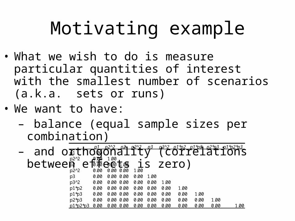
• What we wish to do is measure particular quantities of interest with the smallest number of scenarios (a.k.a. sets or runs)

• We want to have:– balance (equal sample sizes per combination) – and orthogonality (correlations between effects is

zero)p1 p2^2 p2 p2^2 p3 p3^2 p1*p2 p1*p3 p2*p3 p1*p2*p3

p1 1.00p2^2 0.00 1.00p2 0.00 0.00 1.00p2^2 0.00 0.00 0.00 1.00p3 0.00 0.00 0.00 0.00 1.00p3^2 0.00 0.00 0.00 0.00 0.00 1.00p1*p2 0.00 0.00 0.00 0.00 0.00 0.00 1.00p1*p3 0.00 0.00 0.00 0.00 0.00 0.00 0.00 1.00p2*p3 0.00 0.00 0.00 0.00 0.00 0.00 0.00 0.00 1.00p1*p2*p3 0.00 0.00 0.00 0.00 0.00 0.00 0.00 0.00 0.00 1.00

How may scenarios do we need?If we have a straight linear main effects we the

following tells us how many runs we may need (in SAS):

%mktruns(3 3 3); Some Reasonable

Design Sizes Cannot Be (Saturated=7) Violations Divided By

9 0 18 0 12 3 9 15 3 9 7 6 3 9 8 6 3 9 10 6 3 9 11 6 3 9 13 6 3 9

14 6 3 9

So we may decide to go with n=18 scenarios

Let’s fit a main effects only model%mktdes(factors=x1-x3=3,n=18)proc print; run;

Prediction Design Standard Number D-Efficiency A-Efficiency G-Efficiency Error ƒƒƒƒƒƒƒƒƒƒƒƒƒƒƒƒƒƒƒƒƒƒƒƒƒƒƒƒƒƒƒƒƒƒƒƒƒƒƒƒƒƒƒƒƒƒƒƒƒƒƒƒƒƒƒƒƒƒƒƒƒƒƒƒƒƒƒƒƒƒƒƒ 1 100.0000 100.0000 100.0000 0.6236 2 100.0000 100.0000 100.0000 0.6236 3 98.4771 96.8616 84.3647 0.6336 4 98.4771 96.8616 84.3647 0.6336 5 98.4771 96.8616 84.3647 0.6336 Obs x1 x2 x3

1 3 3 2 2 3 3 1 3 3 2 3 4 3 2 2 5 3 1 3 6 3 1 1 7 2 3 2 8 2 3 1 9 2 2 3 10 2 2 2 11 2 1 3 12 2 1 1 13 1 3 3 14 1 3 3 15 1 2 1 16 1 2 1 17 1 1 2 18 1 1 2

How does this work out?• We have 100% efficiency for the effects we wish to

measure (main effects)• But if we look at the correlation matrix of effects we have

the following:

p1 p2^2 p2 p2^2 p3 p3^2 p1*p2 p1*p3 p2*p3 p1*p2*p3p1 1.00p2^2 0.00 1.00p2 0.00 0.00 1.00p2^2 0.00 0.00 0.00 1.00p3 0.00 0.00 0.00 0.00 1.00p3^2 0.00 0.00 0.00 0.00 0.00 1.00p1*p2 0.00 0.00 0.00 0.00 0.00 -0.35 1.00p1*p3 0.00 0.00 0.00 0.00 0.00 0.00 0.00 1.00p2*p3 0.00 0.00 0.00 0.00 0.00 0.00 0.00 -0.25 1.00p1*p2*p3 0.00 0.00 0.00 0.00 -0.24 0.00 0.00 0.29 0.29 1.00

Is this good enough?

• We see that the main effects are all orthogonal, but we have some correlation between these and the higher order interaction terms. (eg: P3^2 and P1*P3.)

• Is this a problem?

– Well yes and no.• No, if these effects are not of interest (e.g. P1*P3)

– i.e. we suspect they don’t exist in real life.

• Yes, if we suspect they might and/or we or not sure if they do or not.

Is this good enough?…• Well-known fact in almost cases involving real data (Louviere,

Hensher, Swait, 2000)

• Main effects explain the largest amount of variance in respondent data, often 80% or more (70-90%);

• Two-way interactions account for the next largest proportion of variance, although this rarely exceeds 3%~6%;

• Three-way interactions account for even smaller proportions of variance, rarely more than 2%~3% (usually 0.5%~1%);

• Higher-order interactions account for minuscule proportions of variance.

Let’s fit a model with main effects with 2nd order interactions

%mktdes(factors=x1-x3=3, interact = x1*x2 x1*x3 x2*x3 x1*x2*x3 ,n=18)

proc print; run; Design Standard Number D-Efficiency A-Efficiency G-Efficiency Error ƒƒƒƒƒƒƒƒƒƒƒƒƒƒƒƒƒƒƒƒƒƒƒƒƒƒƒƒƒƒƒƒƒƒƒƒƒƒƒƒƒƒƒƒƒƒƒƒƒƒƒƒƒƒƒƒƒƒƒƒƒƒƒƒƒƒƒƒƒƒƒƒ 1 0.0000 0.0000 0.0000 0 2 0.0000 0.0000 0.0000 0 3 0.0000 0.0000 0.0000 0 4 0.0000 0.0000 0.0000 0 5 0.0000 0.0000 0.0000 0

p1 p2^2 p2 p2^2 p3 p3^2 p1*p2 p1*p3 p2*p3 p1*p2*p3p1 1p2^2 -0.1 1p2 0 0 1p2^2 0.09 -0.22 0 1p3 -0.1 -0.07 -0.3 -0.06 1p3^2 -0 0.12 0.17 -0.06 -0.04 1p1*p2 0 0 0 0 0.14 0.26 1p1*p3 -0.1 -0.09 0.12 -0.08 -0.11 -0.06 -0.569 1p2*p3 0.11 -0.28 -0.1 -0.25 0.09 -0.17 -0.196 0.124 1p1*p2*p3 -0.6 0.14 -0.2 0.12 0.17 0.09 -0.291 0.233 -0.19 1

So how do we do now?

• This is an unmitigated disaster when we only have 18 scenarios.

• So let’s change the number of scenarios we investigate.

• We can increase this to 27 – as this is divisible by 3x3 = 9 – i.e. every possible combination for two 3 level

factors

Let’s fit a model with main effects with 2nd order interactions (27 scenarios)

%mktdes(factors=x1-x3=3, interact = x1*x2 x1*x3 x2*x3 x1*x2*x3 ,n=27)

proc print; run; Design Standard Number D-Efficiency A-Efficiency G-Efficiency Error ƒƒƒƒƒƒƒƒƒƒƒƒƒƒƒƒƒƒƒƒƒƒƒƒƒƒƒƒƒƒƒƒƒƒƒƒƒƒƒƒƒƒƒƒƒƒƒƒƒƒƒƒƒƒƒƒƒƒƒƒƒƒƒƒƒƒƒƒƒƒƒƒ 1 100.0000 100.0000 100.0000 1.0000 2 100.0000 100.0000 100.0000 1.0000 3 100.0000 100.0000 100.0000 1.0000 4 100.0000 100.0000 100.0000 1.0000 5 100.0000 100.0000 100.0000 1.0000

p1 p2^2 p2 p2^2 p3 p3^2 p1*p2 p1*p3 p2*p3 p1*p2*p3p1 1.00p2^2 0.00 1.00p2 0.00 0.00 1.00p2^2 0.00 0.00 0.00 1.00p3 0.00 0.00 0.00 0.00 1.00p3^2 0.00 0.00 0.00 0.00 0.00 1.00p1*p2 0.00 0.00 0.00 0.00 0.00 0.00 1.00p1*p3 0.00 0.00 0.00 0.00 0.00 0.00 0.00 1.00p2*p3 0.00 0.00 0.00 0.00 0.00 0.00 0.00 0.00 1.00p1*p2*p3 0.00 0.00 0.00 0.00 0.00 0.00 0.00 0.00 0.00 1.00

Conclusions

• Try to keep the number of scenarios (runs, sets) to less than 40 max. – otherwise you get respondent fatigue

• Only measure effects up to 2nd order (3rd order and above are difficult to explain and don’t account for much explanation

• If you have prior knowledge of which effects are more likely than others, then use this to establish which effects you want to measure.