NBER WORKING PAPER SERIES

SHORT-RUN SUBSIDIES AND LONG-RUN ADOPTION OF NEW HEALTH PRODUCTS:EVIDENCE FROM A FIELD EXPERIMENT

Pascaline Dupas

Working Paper 16298http://www.nber.org/papers/w16298

NATIONAL BUREAU OF ECONOMIC RESEARCH1050 Massachusetts Avenue

Cambridge, MA 02138August 2010

I am grateful to Christian Hellwig and Adriana Lleras-Muney for detailed suggestions, and to SandraBlack, Sylvain Chassang, Jessica Cohen, Esther Duflo, Giacomo De Giorgi, Frederico Finan, SeemaJayachandran, Robert Jensen, Rohini Pande, Jonathan Robinson, Justin Sydnor, and numerous seminarparticipants for helpful comments and discussions. I thank Katharine Conn, Moses Baraza, and theirfield team for their outstanding project implementation and data collection. The study was fundedby the Acumen Fund, the Adessium Foundation, the Exxon Mobil Foundation, a Dartmouth FacultyBurke Award and UCLA. The Olyset nets used in the study were donated by Sumitomo Chemical.All errors are my own. The views expressed herein are those of the author and do not necessarily reflectthe views of the National Bureau of Economic Research.

NBER working papers are circulated for discussion and comment purposes. They have not been peer-reviewed or been subject to the review by the NBER Board of Directors that accompanies officialNBER publications.

© 2010 by Pascaline Dupas. All rights reserved. Short sections of text, not to exceed two paragraphs,may be quoted without explicit permission provided that full credit, including © notice, is given tothe source.

Short-Run Subsidies and Long-Run Adoption of New Health Products: Evidence from a FieldExperimentPascaline DupasNBER Working Paper No. 16298August 2010JEL No. C93,D12,H42,O33

ABSTRACT

Short-run subsidies for health products are common in poor countries. How do they affect long-runadoption? We present a model of technology adoption in which people learn about a technology'seffectiveness by using it (or observing others using it) for some time, but people quit using it too earlyif they face higher-than-expected usage costs (e.g., side effects). The extent to which one-off subsidiesincrease experimentation, and thereby affect learning and long-run adoption, then depends on people'spriors on these usage costs. One-off subsidies can also affect long-run adoption through reference-dependence:People might anchor around the subsidized price and be unwilling to pay more for the product later.We estimate these effects in a two-stage randomized field experiment in Kenya. We find that, for anew technology with a lower usage cost than the technology it replaces, short-run subsidies increaselong-run adoption through experience and social learning effects. We find no evidence that peopleanchor around subsidized prices.

Pascaline DupasDepartment of EconomicsUCLA8283 Bunche HallLos Angeles, CA 90095and NBERpdupas@econ.ucla.edu

1 Introduction

Between nine and ten million children under age �ve die every year, most of them in developing

countries.1 It is estimated that nearly two thirds of these deaths could be averted using existing

preventative technologies, such as vaccines, insecticide-treated materials, vitamin supplementa-

tion, or point-of-use chlorination of drinking water.2 An important question yet to be answered

is how to increase adoption of these technologies.

A commonly proposed way to increase adoption in the short run is to distribute those

essential health products for free or at highly subsidized prices (WHO, 2007; Sachs, 2005).

There are two main reasons to do so. First, given the infectious nature of the diseases they

prevent, most of these products generate positive health externalities, and private investment

in them would be socially suboptimal without a subsidy. Second, when the majority of the

population is poor and credit-constrained, subsidies might be necessary to ensure widespread

access (Cohen and Dupas, 2010).

For some products, such as vaccines, one-time adoption is su¢ cient to generate important

health impacts. One-time subsidies are well-suited for such technologies. But for other products,

such as anti-malarial bednets, water treatment kits, or condoms, repeated adoption over time

is required to generate the hoped-for health impacts. A key question and ongoing debate is

whether one-time subsidies for such technologies increase or dampen private investments in

them in the long run.

Free or highly subsidized distribution of a product in the short run may increase demand in

the long run if the product is an experience good. Bene�ciaries of a free or highly subsidized

sample will be more willing to pay for a replacement after experiencing the bene�ts and learning

the true value of the product if they previously had underestimated these bene�ts. This learning

might trickle down to others in the community (those ineligible for the subsidy) and increase the

overall willingness to pay in the population as knowledge of the true value of the product di¤uses.

Furthermore, if short-run adoption of the product leads to positive health and productivity

e¤ects, bene�ciaries of a subsidized sample might have more cash-on-hand to invest in sustained

adoption.

1Black et al, 2003.2Jones et al., 2003.

1

These positive e¤ects hinge upon people�s making use of a product or technology that they

receive for free or at a highly subsidized price. This might not be the case, however. Households

that are not willing to pay a high monetary price for a product might also be unwilling to pay

the non-monetary costs associated with using the product on a daily basis (Chassang, Padro i

Miquel and Snowberg, 2009; Ashraf, Berry and Shapiro, forthcoming).

Furthermore, consumers could take previously encountered prices as reference points, or

anchors, which would a¤ect their subsequent reservation price (Koszegi and Rabin, 2006). Such

e¤ects, known in psychology as �background contrast e¤ects�and �rst identi�ed experimentally

by Simonson and Tversky (1992), have recently been observed outside the lab by Simonsohn

and Loewenstein (2006). Under such reference-dependent preferences, subsidies could generate

an �entitlement e¤ect�: those who receive a subsidy for a health product may anchor around

the subsidized price and be unwilling to pay a higher price for the product once the subsidy

ends or is reduced.

The view that these negative e¤ects might dominate the standard positive learning e¤ects is

quite prevalent among development practitioners. As the Boston Globe summarized: �The Holy

Grail of international development has long been sustainability � [...] for several decades it�s

been the conventional wisdom that unless people spend money on something they will be unlikely

to value it �or use it. Give things away and they will be taken for granted, it�s thought.�3 For

example, the non-pro�t organization One Acre Fund, working with rural households in East

Africa, lists as its core value: �We don�t give handouts - we empower permanent life change.

Lasting change must rely on the poor themselves.�4 There is, however, no rigorous evidence to

date as to what short-run subsidies do to long-run adoption of new technologies.

This paper aims to inform this debate in two steps. First, we provide a model for under-

standing the role of prices in the adoption of technologies for which adoption requires not only

acquisition, but also repeated usage of the technology once acquired. We generate predictions

as to the circumstances and technology characteristics under which short-run subsidies will

increase the long run level of adoption. Second, we test the predictions of the model through a

�eld experiment for one speci�c technology (long-lasting antimalarial bednets) in one speci�c

3Christopher Shea, �A Hand Out, not a Hand Up�, November 2007. Article retrived on 12/13/2009 athttp://www.boston.com/news/education/higher/articles/2007/11/11/a_handout_not_a_hand_up/

4Retrieved on March 2, 2009 at this link: http://www.oneacrefund.org/how_it_works/core_values

2

set of circumstances.

The key feature of our model is that households are uncertain about two elements of a

newly introduced health technology or health product: the e¤ectiveness of the product, and its

non-monetary cost of usage (for example, how �hot�it is to sleep under a bednet, or how bad

a deworming pill tastes). People immediately learn the cost of usage upon buying the product,

say by using the product for one day. In contrast, learning about the e¤ectiveness takes some

time: people who use the product receive (publicly observable) signals about its e¤ectiveness,

but these signals are imprecise, in particular in environments where individual-speci�c health

shocks are common. In this context, we show that subsidies may have no e¤ect on the adoption

of the product if people initially underestimate its non-monetary usage cost. This is because

subsidies a¤ect the purchase decision of households who have a low prior about the product�s

e¤ectiveness. These households will likely not use the product once they learn its true usage

cost. In this context, higher subsidies may not generate additional signals about the product�s

e¤ectiveness and therefore may not a¤ect the dynamic adoption process. In contrast, subsidies

will increase the level of experimentation and thus learning about the new product if people

initially overestimate the non-monetary usage cost. This, in turn, will speed up the di¤usion

process and increase long-run adoption, unless people exhibit reference-dependent preferences

and anchor around subsidized prices.

To test these predictions, we conducted a �eld experiment in Kenya with a new technol-

ogy whose non-monetary usage cost was likely overestimated by households at baseline. The

technology we introduced is the Olyset long-lasting insecticide-treated bed net (LLIN), a recent

innovation in malaria control. The Olyset LLIN is signi�cantly more comfortable to sleep un-

der than traditional bednets, and also more e¤ective in the long run. The experiment involved

1,120 households in Kenya and included two phases. In Phase 1, subsidy levels for Olyset LLINs

were randomly assigned across households within six villages. Households had three months

to acquire the LLIN at the subsidized price they had been assigned to. Prices varied from $0

to $3.80, which is about twice the average daily wage for casual agricultural work in the study

area. In Phase 2, a year later, all households in four villages were given a second opportunity

to acquire an Olyset LLIN, but this time everyone faced the same price ($2.30). Phase 2 was

unannounced, therefore at the time individuals made their purchasing decision in Phase 1, they

were not aware that they would receive a second chance to acquire the product a year later.

3

The LLIN was not available outside of the experiment, but traditional nets were available on

the market at the retail price of $1.50.

This experimental design allows us to test multiple predictions about the e¤ects of temporary

subsidies on demand, both over time and across individuals.

We �rst test whether subsidies increased the level of experimentation. We �nd very strong

evidence for this prediction, consistent with the fact that the new technology introduced was

less costly to use than households anticipated. We then test whether this higher level of exper-

imentation led to positive or negative updating about the private returns to LLIN use. To this

end, we examine how full or very large subsidies for an LLIN in Phase 1 a¤ect willingness to

pay for an LLIN in Phase 2. We �nd that gaining access to a free or highly subsidized LLIN in

the �rst year increases households�reported as well as observed willingness to pay for an LLIN

a year later. This suggests the presence of a learning e¤ect which dominates any potential

anchoring e¤ect. We then test speci�cally for the presence of anchoring. We �nd some evidence

of anchoring at higher prices, but no anchoring around zero or very low prices. Overall, our

evidence suggests important learning-by-doing e¤ects among subsidy receipients.

We then turn to studying the social e¤ects of subsidies. To avoid the classic re�ection

problem in the estimation of social e¤ects (Manski, 1993), we exploit the exogenous variation

in the density of households who received a free or highly subsidized LLIN in Phase 1 as a

source of exogenous variation in exposure to signals about the returns to using the product.

We �nd that households facing a positive price in Phase 1 were more likely to purchase the

LLIN when the density of households around them who received a free or highly subsidized

LLIN was greater, suggesting social learning e¤ects.

Overall, our results suggest that, consistent with the model prediction given the character-

istics of the technology studied, the total e¤ect of short-run subsidies on long-run adoption of

LLINs is positive. Previously encountered prices matter, but more so through their e¤ect on

available knowledge about the product than through entitlement e¤ects.

The model helps reconcile our �ndings with those of two previous studies, Ashraf, Berry

and Shapiro (forthcoming) and Kremer and Miguel (2007), which both found results somewhat

opposite to ours. Ashraf, Berry and Shapiro �nd that subsidies for a water chlorination product

in urban Zambia increased the rate of purchase but did not increase the overall rate of exper-

imentation with the product. Their result is consistent with the case of our model in which

4

people underestimate the cost of using chlorine at the time they make the decision to purchase

it (e.g., they underestimate the chlorinated taste of the water). In that case, those induced to

purchase the product by a subsidy are not motivated to use it once they learn its true usage

cost.

Kremer and Miguel (2007) use a randomized evaluation of a school-based deworming pro-

gram in Kenya to estimate the role of peer e¤ects in health technology adoption. They �nd

that households were less likely to invest in deworming if they had a higher number of social

contacts who bene�tted from free deworming in the past. Their negative e¤ect is also con-

sistent with our model. Deworming pills generate important negative side e¤ects, making the

non-monetary cost of deworming relatively high. Households in the Kremer and Miguel study

likely underestimated these costs initially. Subsidies for deworming enabled households to learn

the true usage cost of deworming and revise their beliefs about the private returns to using the

drug downwards, thus leading to lower long-run adoption.

Our �ndings also help shed light on the Kremer and Miguel (2007) result that parents

in Kenya who were exposed to free deworming treatment for their children for a year were

extremely unwilling to pay for deworming once it stopped being free. Their experimental

design did not allow a test of whether this drop was due to �entitlement� e¤ects or to low

perceived private returns of deworming. Our results, based on data from the same area of

Kenya, suggest that entitlement e¤ects likely played a negligible role in the demand drop that

they observed following the price increase.

Our paper contributes to a growing literature on the role of learning-by-doing and social

learning in technology adoption in poor countries. The evidence so far, mostly non-experimental

and mostly focused on agricultural technologies, is rather mixed and suggests that the role of

social learning is likely to vary greatly with the context and the product considered.5 Our paper

5Foster and Rosenzweig (1995) and Besley and Case (1997) �nd that a farmer�s ability to reap pro�ts froma new technology increases with not only her own but also her neighbors�experience with the new technology,but Munshi (2004) �nds that social learning requires a certain degree of homogeneity among farmers, andBandiera and Rasul (2006) �nd some evidence of strategic delay in adoption of new products. Conley andUdry (forthcoming) present evidence that social learning is important in the di¤usion of knowledge regardingpineapple cultivation in Ghana, while the randomized experiment of Du�o, Kremer and Robinson (2009) �ndsno social learning in fertilizer use in Western Kenya. There are few empirical studies of social learning outsideagriculture. Behrman et al. (2001) study social networks of young women in rural Kenya and �nd evidence of S-shaped di¤usion of attitudes and behaviors with respect to contraception and AIDS. Munshi and Myaux (2006)provide suggestive evidence from India that a woman�s contraception decision responds strongly to changes incontraceptive prevalence in her own religious group within the village but not to changes outside her religious

5

also contributes to the empirical �psychology and economics� literature, testing behavioral

economics in the �eld (see DellaVigna, 2009, for a review), and complements earlier papers

that have estimated, in rich countries, how the willingness to pay for a product can be a¤ected

by anchors (Ariely, Loewenstein and Prelec, 2003), previously encountered prices (Simonsohn

and Loewenstein, 2006; Mazar, Koszegi and Ariely, 2009), or the range of options available

(McFadden, 1999; He¤etz and Shayo, 2009). Finally, our paper makes a contribution to the

literature on experimentation and experience goods pricing (Bergemann and Valimaki, 2000,

2006).

The remainder of the paper is as follows. Section 2 presents a model of technology adoption

in the presence of ex-ante uncertainty about both the e¤ectiveness of the technology and its

usage cost. Section 3 presents some background information on malaria and the preventative

technology studied in the application, and then describes the experimental design. Section 4

presents the results on the direct e¤ect of subsidies, and Section 5 presents the results on their

indirect e¤ects via social learning. Section 6 concludes.

2 Theoretical Framework

This section presents a general framework for understanding the adoption of a new preventative

health technology. The goal is to clarify the potential channels through which a one-time subsidy

can change the long-run level of adoption, and to provide empirically implementable tests of

their relative importance. We use an experimentation model similar to those in Moscarini

(2005) and Moscarini and Smith (2001).

We consider a technology for which health-e¤ective adoption requires not only acquiring the

technology, but also repeatedly using it over its lifespan. In addition to anti-malarial bednets

(which can last for 3-4 years and are supposed to be used nightly), examples of such technologies

include water chlorination products (typically sold in bottles large enough to treat a 6-member

household�s drinking water daily for 1 month), iron pills (sold in bulk), or water �lters (that

have a lifespan of 6 months and should be used daily). We consider that, at the time households

decide whether to acquire the technology, they are uncertain about both the e¤ectiveness of

network. Oster and Thornton (2009) �nd evidence of peer e¤ects in the usage of a new female hygiene productprovided for free.

6

the technology and the cost associated with using the technology. Households have two sources

of information: their own experimentation with the technology, and the experience of their

neighbors. Learning about the usage cost is relatively quick upon ownership of the technology

(one only needs to use it a few times to learn its usage cost), but learning about the health

e¤ectiveness takes time, as households receive only noisy signals.

2.1 Set-up

2.1.1 Information

Bene�ts The average e¤ectiveness � of a new health technology is ex�ante uncertain.

Individuals have a prior belief on �, concentrated on two points: p0 = Pr(� = 1) = 1� Pr(� =

0) 2 (0; 1); where � = 1 if the technology is �good� (i.e., more e¤ective than the status quo

technology by 1 util-equivalent), and � = 0 if the technology is �bad�(i.e., not more e¤ective

than the status quo technology.)

If households own and use the technology, they get a signal about its quality. The signal

is subject to idiosyncratic noise that keeps � hidden and creates the inference problem. We

consider that it is a normal random variable, a Brownian Motion with drift � and known

variance �2: Over time, individuals observe the signals hXti ; generating a �ltration�FXt

; and

update their belief in a Bayesian fashion from the prior p0 to the posterior pt � Pr(� = 1jFXt ):

The Brownian di¤usion is characterized by:

E(dpt) = 0

E(dp2t ) = (1

�)2p2t (1� pt)

2dt

where 1�is the signal-to-noise ratio.

To update beliefs, households use both their own experience and that of J neighbors. We

consider that each household i has a location on a two-dimensional map, and that J signals

are drawn from the set of households within a distance d in each direction. If a fraction wit

of households in this radius experimented (i.e., bought and used) the technology in period t,

household i receives witJ signals. We consider that � decreases with the number of signals

received: the more neighbors experiment, the higher the signal to noise ratio.

7

Costs There are two types of costs associated with the technology: the monetary cost of

acquiring the product (price m); and the time and/or utility cost of using it, denoted by c, with

0 < c < 1.

Households readily observe m, but c is uncertain ex-ante. Households� prior on c is a

probability distribution denoted F (:). As soon as they acquire the technology, they learn the

true c. They can also learn c from their neighbors. We consider that each household has a

probability � to learn the true c from each neighboring household that acquired the technology

and learned c: In other words, household i�s belief about c at time t is:

F it (c) =

8>>><>>>:c if i acquired the technology at any time prior to t

c if i learned c from a neighbor

F i0(:) if i never acquired the technology and didn�t learn from any neighbor

9>>>=>>>;If i has witJ neighbors who acquired the technology at time t; the likelihood that household

i hasn�t learned c from a neighbor by time t is (1� �)witJ :

2.1.2 Payo¤s

Time is continuous and the interest rate is r. Conditional on owning the technology and using

it, and given the belief pt about the e¤ectiveness, a household�s expected instantaneous payo¤at

time t is �t = pt�c: The household�s value of using the technology if it is good with probability

pt solves the Bellman equation:

V1(pt; c) = r�(pt; c)dt+ (1� rdt) � E(V1(pt + dpt; c))

Applying Ito�s lemma: V1(pt + dpt; c) = V1(pt) + V 01(pt)E(dpt)+ 1

2V 001 (pt)E(dp2t ), we obtain

the following ordinary di¤erential equation:

rV1(pt; c) = r(pt � c) +1

2p2t (1� pt)

2 1

�41V 001 (pt; c)

The �rst term represents the current payo¤, and the second term corresponds to the option

value of experimenting: the speed of learning 12p2(1�p)2 1

�4is converted into payo¤ units by the

convexity of V 001 (pt); because information spreads posterior beliefs and empowers more informed

8

decisions later on.

Households that don�t experiment themselves can still learn about the e¤ectiveness from

neighbors. Their value function solves:

rV0(pt; c) =1

2p2t (1� pt)

2 1

�40V 000 (pt; c)

where �0 > �1. In other words, the signal-to-noise ratio is lower when people do not receive

their own signal and purely rely on their neighbors�signals.

2.1.3 Optimal Experimentation (conditional on purchase)

Lemma 1 The value function of the household is an increasing and convex function of p:

V1(p; c) =

�p� c+ (c)p1=2�

p1=4+2r�2(1� p)1=2+

p1=4+2r�2 if p � p(c)

V0(p; c) = 0 if p � p(c)

�

where (c) and the threshold p(c) 2 [0; c] uniquely solve the boundary conditions V1(p) = V0(p) =

0 (value matching) and V 01(p) = V 0

0(p) = 0 (smooth pasting).

The value function V1(p; c�) is drawn in Figure 1A. Below the threshold p, households

choose not to use the technology, even conditional on owning it. For any p � p(c), they use the

technology. The threshold p(c) is lower than the �myopic�threshold c, since the option value

of experimentation make households willing to take a negative current payo¤.

2.1.4 Optimal Purchase Decision

The top panel of Figure 1b plots V1(p; c) as a function of c; for a given prior pt: The function

is decreasing and convex, and shifts outwards as pt increases.

Proposition 1 Call c(p) the inverse of p(c): If the household has the prior pt on the e¤ective-

ness and the prior distribution F (:) on the cost of usage c; the household will buy the technology

at price mt if and only if

mt �Z c(p)

0

V1(pt; c)dF (c)

Since V1(p; c) is increasing in the prior on p; the likelihood of purchase increases with the

prior pt: For a given prior pt, whether a household buys the technology will depend on its prior

9

F (:) on the usage cost. The bottom panel of Figure 1b plots three possible prior distributions.

For a given prior pt, households with prior distribution F1(:) will be willing to pay a higher

price for the technology than households with the prior distributions F2(:) or F3(:):

When the new technology is �rst introduced, the priors p and F (:) might depend on the

availability of comparable technologies. In a context like the one in which conducted our �eld

experiment, where the status quo technology is already relatively good and the new technology

is similar to the old technology (e.g., the status quo technology is an insecticide-treated net and

the new technology is a long-lasting insecticide treated net), individuals may have relatively

optimistic priors about the e¤ectiveness of the new technology. In contrast, for technologies

that are radically new (e.g., in that they rely on unknown scienti�c principles), individuals

might start with pessimistic beliefs (low p) and adoption might be very limited, unless the

technology is heavily subsidized for at least some individuals. A good example is that of

insecticide-treated curtains, that provide the insecticide halo necessary to repel mosquitoes but

do not provide the intuitive �physical barrier�against mosquitoes that people tend to think is

the critical component of a bed net.

2.2 Static E¤ects of Price Subsidies on Experimentation Level

The dynamic e¤ects of price subsidies will depend on their static e¤ects on the level of ex-

perimentation: the more households experiment with the technology, the faster the learning

about e¤ectiveness will be. In our model, the e¤ect of a price subsidy on the total amount of

experimentation (and hence learning) is never going to be negative, but it might not be strictly

monotonic. Here is why:

A subset SA of households that get enticed to buy the product by the subsidy will experiment

with the product once they have it: those are the households that initially overestimate the usage

cost. Indeed, for a given prior on the e¤ectiveness p, lower prices crowd in people with higher

priors on the usage cost c: Those who get surprised by a realized usage cost c� lower than

expected can only increase their level of experimentation as a result.

On the other hand, a subset SB of households that get enticed to buy the product by the

subsidy will not experiment with the product once they have it: those are the households that

initially underestimate the usage cost. Indeed, for a given prior on c, lower prices crowd in

10

people with lower priors on p: Those who get surprised by a realized usage cost c� that is

higher than expected will not experiment if their prior on the e¤ectiveness is too low, namely

if p � p(c�):

Overall, this suggests that the share of households that experiment with the product among

those who acquire it might not be a monotonic function of the subsidy level. As a result, short-

run adoption (and hence learning) might not be strictly increasing in the subsidy level. In

particular, if SA = f?g for subsidy levels above a certain threshold, then any further increase

in the subsidy above that threshold would not lead to any increase in experimentation: the level

of experimentation would level o¤.6

In the �eld experiment below, we �nd that adoption (acquisition + experimenation) is

strictly increasing with the subsidy level (strictly decreasing with the price level). We take it as

evidence that, in our context, the subset SA is not empty. In addition, we �nd that the share

of people experimenting with the technology (among those who own it) does not decrease with

the subsidy level. This implies that the subset SA is larger than the subset SB : people tended

to overestimate the usage cost of our technology at baseline, rather than underestimate it, and

therefore high subsidies increased immediate adoption and learning.

In contrast, Ashraf, Berry and Shapiro (forthcoming) �nd that higher subsidies increased

the fraction of people who acquired a water chlorination product but did not use it. This

suggests that, in their context, subset SB was larger than subset SA : a relatively large fraction

of people underestimated the cost of using chlorine in their water (they underestimated how

bad their water would taste if they used chlorine), and as a result, they chose not to experiment

once they learned the true usage cost.

2.3 Dynamic E¤ects

We have shown that the magnitude of the static e¤ect of subsidies on the level of experimenta-

tion (and thus learning) will depend on the priors�distributions. This implies that the dynamic

e¤ect of subsidies on adoption will also depend on the priors. But besides the learning e¤ect,

6The prior belief about the e¤ectiveness of the product could also be an increasing function of the observedprice (Bagwell and Riordan, 1991). If people face di¤erent prices, they might start with heterogeneous priors.We abstract from this here, and shut down this mechanism in the experiment by informing everyone of theunsubsidized price. Alternatively, the prior belief about the e¤ectiveness could be an increasing function of thesubsidy size. If so, the experimentation level would strictly increase with the subsidy level.

11

there are two additional dynamic e¤ects through which short-run subsidies might a¤ect longer-

run demand: an anchoring e¤ect and an income e¤ect. Below, we �rst describe these e¤ects,

and then describe what our empirical tests can tell us about them.

2.3.1 Anchoring E¤ect

Let�s now consider that the utility of individual i is composed of two additive terms: intrinsic

utility and gain-loss utility. Intrinsic utility is a function of absolute outcomes. Gain-loss utility

captures reference-dependence. Following K½oszegi and Rabin (2006), we formalize reference-

dependence as follows. Denote m̂it household i�s reference price for the technology at time t,

then paying a price mt for the technology generates gain-loss utility r(m̂it �mt): To allow for

loss aversion, we allow the function r to be kinked at zero. For example, r could be two-piece

linear, with a slope �G � 0 for gains (when m̂it � mit), and a slope of �L � �G for losses (when

m̂it < mit).

The decision to purchase the bednet is now slightly modi�ed compared to proposition 2.

Proposition 2 At any period t, given reference price m̂it, household i will buy the technology

at price mt if and only if

mt �Z c(p)

0

V (p0; c)dF (c) + r(m̂it �mt)

This means that, for a given set of priors p and F (c), households who face a price higher

(lower) than their reference point for the technology will be less (more) likely to purchase it

than those who face a price equal to their reference point.

We consider that the reference price m̂it evolves as follows. We assume that prior to the

introduction of the technology, all households have a common reference point p̂0, based on the

cost of the status quo technology. After the new technology is introduced in period k, we

suppose that household i revises its reference price to m̂i;k+t = pik;8t � 1. In other words, the

household �anchors�around the �rst o¤er price it receives.

12

2.3.2 Income (via Health) E¤ect

If the health technology is e¤ective, households who experiment with it are likely to get healthier

over time. This positive health e¤ect could a¤ect disposable income in two ways. First, healthier

households are likely to be more productive and able to generate higher income. Second,

healthier households are likely to spend less on malaria treatment expenditures. If subsidies

increase the rate of adoption of the new health technology, they might thus increase disposable

income as a result.

In addition, for many health technologies, adoption by some households generates positive

health externalities for others. For example, in the case of malaria, having more neighbors

using a protective device such as a bednet reduces one�s own chance of infection (since malaria

is transmitted from human to human). There might thus be an indirect e¤ect of subsidies on

the health (and thus income) level of those not directly targeted by the subsidy.

2.3.3 Overall direct e¤ect of one-time subsidies on long-run adoption

For household i, the impact of having faced price mit in period t on the household�s reservation

price mi at a subsequent period t+�t (when the price has become mi;t+�t > mi;t) is the sum

of three e¤ects:

@mi;t+�t

@mi;t

= learning + anchoring + income

The �rst e¤ect is learning-by-doing about the technology�s e¤ectiveness and its usage cost.

For both parameters, the learning e¤ect can be zero if the price in period t is such that household

i does not acquire the product and does not experiment with the product between time t and

time t + �t. If the household acquires the product and experiments with it, the learning

e¤ect will be positive or negative depending on whether the household�s initial priors were

overestimates or underestimates. The second e¤ect is the anchoring e¤ect, which is positive or

zero. The third e¤ect is the income e¤ect, which is negative or zero. The income e¤ect can

result from the health e¤ect, or from a mechanical e¤ect of the subsidy on the intertemporal

budget constraint: those who paid more for the technology in period t have less money available

to invest in the technology again in period t+�t.

In the experiment below, we �nd a negative e¤ect of the period t price on willingness to pay

13

at t + �t. In other words, we �nd that the sum of the three e¤ects in the equation above is

negative. We take it as evidence that the anchoring e¤ect is at best modest, and overwhelmed

by the sum of learning and income e¤ects. We then speci�cally test for the presence of anchoring

and �nd no evidence of anchoring around zero or very low prices. We also speci�cally test for

the presence of an income e¤ect, and �nd inconclusive evidence. Overall, our results suggest

that the main e¤ect through which short-run subsidies a¤ect later adoption is a learning e¤ect,

which in our context appears positive (people learned the technology was better than what they

initially thought).

2.3.4 Overall indirect e¤ect of one-time subsidies on long-run adoption

For household i, the impact of having a given share s�i;t of neighbors that receive a high subsidy

level in period t on the household�s reservation price mi at a subsequent period t + �t is the

sum of three e¤ects:

@mi;t+�t

@s�i;t= learning + income + free-riding

The �rst e¤ect represents social learning about the technology�s e¤ectiveness and its usage cost.

The larger the number of neighbors who receive a low price, the larger the number of neighbors

who acquire the product and learn the usage cost. If those neighbors are �badly�surprised by

the usage cost and do not experiment with the product (they belong to subset SB), there will

be no learning about the e¤ectiveness. But if neighbors experiment with the product, the faster

the learning about the e¤ectiveness (the higher the signal-to-noise ratio). This social learning

e¤ect will induce higher or lower adoption in the future depending on whether the household

prior pt was too optimistic or too pessimistic to start with.7 The other two e¤ects come from

the positive health externality. One one hand, having more neighbors experimenting with the

product can increase one�s own health and thus productivity level and income realization. This

corresponds to the second e¤ect, which is likely to be positive. On the other hand, the returns

7Having more neighbors that own the product but do not use it (i.e., more neighbors in subset SB) couldactually lead to �mislearning�, if people only know their neighbors�ownership status and not their usage status.In other words, if household A knows that neighboring household B owns the product but doesn�t know thatB is not using the product, household A might think that it receives signals on the e¤ectiveness by observinghousehold B�s health level. This would lead household A to incorrectly revise its belief about the e¤ectivenessdownwards.

14

to using the product oneself are lower if one bene�ts from one�s neighbors� own protective

behavior. This could lead one to free ride �the third e¤ect, which is likely to be negative.

In the experiment below, we �nd a positive social e¤ect overall (the sum of the three e¤ects

is positive). We take it as evidence that information e¤ects are positive and that the health

externality is either too small, or too unobservable by individuals, to generate a free-riding

e¤ect that can dominate the learning e¤ect.

3 Experimental Set-Up and Design

3.1 Background on Insecticide-Treated Nets

Over the past two decades, the use of insecticide-treated nets (ITNs) has been established

through multiple randomized trials as an e¤ective and cost-e¤ective malaria control strategy

for sub-Saharan Africa (Lengeler, 2004). But coverage rates with ITNs remain low. Until

recently, one of the key challenges to widespread coverage with ITN was the need for regular

re-treatment with insecticide every 6 months, a requirement few households complied with

(D�Alessandro, 2001). This problem was solved recently through a scienti�c breakthrough:

long-lasting insecticidal nets (LLINs), whose insecticidal properties last at least as long as the

average life of a net (4-5 years), even when the net is used and washed regularly. The �rst

prototype LLIN, the Olyset R Net, was approved by WHO in 2001, but did not get mass

produced until 2006. At the time this study started in Kenya in 2007, the Olyset Net, the

LLIN used in this experiment, was not available for sale, and its e¤ectiveness�relative to that

of regular ITNs available for sale�was unknown.

More speci�cally, at the time of the experiment, the �status quo�technology that households

in Kenya had access to was a regular ITN, subsidized by Population Services International (PSI).

Pregnant women and parents of children under-�ve could purchase an ITN for the subsidized

price of Kenyan shillings (Ksh) 50 ($0.75) at health facilities, and the general population could

purchase ITNs for the subsidized price of Ksh 100 ($1.50) at local stores.

In our study sample, 80% of households owned at least one bednet (of any kind) at baseline,

but given the large average household size, the coverage rate at the individual level was still low,

with only 41% of household members regularly sleeping under a net. About 33% of households

15

had an LLIN of the brand PermaNet R at baseline. The PermaNet LLINs were received free

from the government during a mass distribution scheme targeting parents of children under 5

and conducted in conjunction with the measles vaccination campaign of July 2006, ten months

before the onset of this study. These PermaNets di¤er substantially from the Olyset LLIN

used in our experiment: they are circular and not rectangular, made of polyester and not

polyethylene, and have a smaller mesh. They cannot be distinguished from traditional re-

treatable ITNs with the naked eye, while Olyset nets can. Finally, Olyset nets have been

judged to be less uncomfortable to sleep under than either traditional ITNs or LLINs of the

brand PermaNet, thanks to the wider mesh that enables more air to go through (making the

area under the net less hot).

3.2 Experimental Design: Phase 1

The experiment was conducted in Busia District, Western Kenya, where malaria transmission

occurs throughout the year. The study involved 1,120 households from six rural areas. Par-

ticipating households were sampled as follows. In each area, the school register was used to

create a list of households with children.8 Listed households were then randomly assigned to a

subsidy level for an LLIN. The subsidy level varied from 100% to 40%; the corresponding �nal

prices faced by households ranged from 0 to 250 Ksh, or at the prevailing exchange rate of 65

Ksh to US$1 at the time, from 0 to US$3.8.9 Seventeen di¤erent prices were o¤ered in total,

but each area, depending on its size, was assigned only four or �ve of these 17 prices. Thus,

if an area was assigned the price set {Ksh 50, 100, 150, 200, 250}, all the study households in

the area were randomly assigned to one of these �ve prices according to a computer-generated

random number. All price sets included high, intermediate, and low subsidy levels. However,

the lowest price o¤ered in a given area was randomly varied across areas, and drawn from the

following set: {0, 40, 50, 70}. Only two areas had a price set that included free distribution for

some households.

8Since Kenya introduced Free Primary Education in 2003, school participation is high. The net primaryenrollment rate was estimated at 80% in 2005 and is probably higher now.

9A few years prior to this study, the Kenya Central Bureau of Statistics and the World Bank estimatedthat 68% of individuals in Busia district (the area of study) live below the poverty line, estimated at $0.63 perperson per day in rural areas (the level of expenditures required to purchase a food basket that allows minimumnutritional requirements to be met) (Central Bureau of Statistics, 2003).

16

After the random assignment to subsidy levels had been performed in o¢ ce, trained enu-

merators visited each sampled household. A baseline survey was administered to the female

and/or male head of each consenting household.10 At the end of the interview, the respondent

was given a discount voucher for an LLIN corresponding to the randomly assigned subsidy

level. The voucher indicated (1) its expiration date, (2) where it could be redeemed, (3) the

�nal (post-discount) price to be paid to the retailer for the net, and (4) the recommended

retail price and the amount discounted from the recommended retail price.11 Vouchers could

be redeemed at participating local retailers (1 per area). The six participating retailers were

provided with a stock of blue, extra-large, rectangular Olyset nets. At the time of the study,

extra-large Olyset nets were not available to households through any other distribution channel,

which facilitated tracking of the LLINs that were sold as part of the study.

The participating retailers received as many Olysets as vouchers issued in their community,

and no more. They were not authorized to sell the study Olysets to households outside the

study sample. For each redeemed voucher, the retailers were instructed to note the voucher

identi�cation number and the date of redemption in a standardized receipt book designed for

the experiment. The list of redeemed vouchers and the vouchers stubs themselves were collected

from retailers every 2 weeks.12

The subset of households who had redeemed their LLIN voucher were sampled for a short-

run follow-up administered during an unannounced home visit 2 months on average after the

voucher had been redeemed. During the follow-up visit, enumerators asked to see the net that

was purchased with the voucher, so as to ascertain that it was a study-supplied Olyset LLIN.

The follow-up survey also checked whether households had been charged the assigned price for

the LLIN. Usage was assessed as follows: (1) whether the respondent declared having started

using the net, and (2) whether the net was observed hanging above the bedding at the time of

10Whether the female head, male head or both were interviewed and given the voucher was randomized acrosshouseholds. It had no e¤ect on take-up. In what follows, all regressions include controls for the randomizedgender assignment.11The fact that the recommended retail price was indicated on the voucher could have dampened the possibility

of anchoring e¤ects. From a policy standpoint, indicating the non-subsidized price on a voucher or product iscostless, therefore estimating the overall e¤ect of subsidies in the presence of full information about the non-subsidized price is the relevant policy parameter.12Participating retailers were not allowed to keep the proceeds of the study Olyset sales. However, as an

incentive to follow the protocol, participating retailers were promised a �xed sum of $75 to be paid uponcompletion of the study, irrespective of the number of nets sold but conditional on the study rules being strictlyrespected.

17

the visit.

Note that, while the main advantage of the Olyset LLIN is its long-lasting property, it can

easily be di¤erentiated from other nets in the short run: it is sturdier than other nets because

it is made of polyethylene (and not polyester) and as mentioned earlier, it is noticeably more

comfortable (less hot) thanks to its wider mesh.

3.3 Experimental Design: Phase 2

In a subset of areas (4 out of 6), a long-run follow-up was conducted 12 months after the

distribution of the �rst LLIN voucher.13 All households in those areas were sampled for the

long-run follow-up (both those who had redeemed their �rst voucher, and those who had not).

Data on the incidence of malaria in the previous month was collected. Households were also

asked if they knew people who had redeemed their vouchers and what those people had told

them about the LLIN acquired with the voucher. In addition, for those who had redeemed the

voucher, usage of the LLIN was recorded as in the �rst follow-up.

At the end of the visit, households received a second LLIN voucher, redeemable at the

same retailer as the LLIN voucher received a year earlier. All households faced the same price

(Ksh150 or $2.30) for this second voucher. The set-up used with retailers was identical to that

used in Phase 1.

By comparing the take-up rate of the second, uniformly-priced voucher across Phase 1 price

groups, we can test whether being exposed to a large or full subsidy dampens or enhances

willingness to pay for the same product a year later. Note, however, that since LLIN have

a lifespan of 4 to 5 years, at the time they received the second LLIN voucher, households

who had purchased an LLIN with the �rst voucher in Phase 1 did not need to replace their

�rst LLIN. The redemption rate of the second voucher thus measures, for those households,

the willingness to pay for an additional LLIN, and not a replacement LLIN. If we make the

reasonable assumption of decreasing marginal returns to LLINs, the willingness to pay observed

through the second voucher redemption will be a lower bound for the willingness to pay for a

replacement LLIN.

13Two areas (randomly selected among the four areas without free distribution) had to be left out at the timeof the long-run follow-up for budgetary reasons.

18

3.4 Verifying Randomization

A baseline survey was administered at households�homes between April and October 2007,

prior to the �rst voucher distribution. The baseline survey assessed household demographics,

socioeconomic status, and bednet ownership and coverage. Table 1 presents summary statistics

on 15 household characteristics, and their correlation with the randomized 1st LLIN price

assignment. Speci�cally, we regress each baseline characteristic on a quadratic in the price

faced in Phase 1 and a set of area �xed e¤ects:

xhj = � 1Phj1 + � 2(Phj1)2 + �j + "hj

where xhj represents a baseline characteristic of household h in area j and Phj1 is the price

faced by household h in Phase 1. We report the coe¢ cient estimates and standard errors for � 1

(column 3) and � 2 (column 4). All of the coe¢ cient estimates are small in magnitude and none

can be statistically distinguished from zero, suggesting that the randomization was successful

at making the price assignment orthogonal to observable baseline characteristics.14

3.5 Verifying Compliance with Study Protocol

All households that redeemed their vouchers declared, when interviewed at follow-up, that they

had been charged the assigned price when they redeemed their voucher at the shop. This

suggests that participating retailers respected the study protocol.

The sales logs kept by participating retailers show that, in total over Phase 1 and Phase 2,

95% of the redeemed vouchers were redeemed by a member of the household that had received

the voucher. Only two of the individuals that redeemed a voucher declared having paid to

acquire the voucher. This suggests that there was almost no arbitrage between households

prior to voucher redemption.

To check for potential arbitrage after redemption (i.e., people selling the LLIN to their

neighbor after having redeemed the voucher), we conducted unannounced home visits and

asked to see the LLIN that had been purchased with the voucher (the study-provided nets

14Alternative speci�cations (linear price e¤ect, dummy for �Free 1st LLIN�, dummies for each price groupsin Figure 1) also show balance across price groups (results available upon request).

19

were easily recognizable). These home visits were conducted after both Phase 1 and Phase

2. Overall, more than 90% of households that had redeemed a voucher could show the LLIN

during the spot check.

4 Results: Learning-by-Doing

4.1 Static E¤ects of Subsidies on Experimentation

The static e¤ects of subsidies on take-up and usage of the Phase 1 LLIN are presented in Figure

2. Panel A shows that the take-up of the �rst voucher is highly sensitive to price: take-up is

quasi-universal for free LLIN vouchers (at 97.5%), but drops to 70 to 55% when the price is

between 40 and 90 Ksh (between $0.6 and $1.4), and further drops to around 30% when the price

crosses the 100 Ksh threshold ($1.5). In contrast, Panel B, which shows usage rates (among

those who redeemed their voucher), suggests that the likelihood that people experimented with

their LLIN does not increase with the price paid.15 As a result, as shown in Panel C, the

adoption rate (take-up + experimentation) drops quite rapidly as the price increases (as the

subsidy level decreases). These results are robust to adding household-level controls (regression

analysis available upon request), and are very similar to those obtained among pregnant women

by Cohen and Dupas (2010).16

In terms of the framework presented in Section 2, these �ndings suggest that most households

that were enticed to buy the LLIN by the subsidy were overestimating the usage cost at baseline.

In other words, subset SA seems much larger in our context than subset SB: In this context,

higher subsidies are likely to generate important learning-by-doing e¤ects: higher subsidies lead

to a much higher share of people experimenting with the product and thereby obtaining a signal

about its e¤ectiveness.

15We group households into �ve price (subsidy) groups to avoid running into small sample problems whenestimating usage rates (especially at higher prices).16Appendix Table A1 shows that attrition at follow-up was not correlated with price, and therefore the

estimates of the e¤ect of price on adoption are unbiased. Appendix Figure A1 shows that, not suprisingly, thetime needed to redeem the voucher increased with price.

20

4.2 Dynamic E¤ects of Subsidies on Long-Run Adoption

4.2.1 Overall E¤ect

This section tests whether households who bene�tted from a free or highly subsidized LLIN in

Phase 1 were more or less willing to pay for a LLIN in Phase 2, when the price was high for

everyone. We test this using both declared preferences and revealed preferences.

First, we look at how households�declared willingness to pay for a bednet was a¤ected by

the subsidy. This is presented in Figure 3, which is restricted to the sample of households that

self-selected into buying the LLIN in Phase 1. Figure 3 presents two averages for each Phase 1

price group: the average willingness to pay for a bednet declared at baseline, before households

had received the �rst voucher; and the average willingness to pay declared at the follow-up,

when households were asked: �If you didn�t have this net, up to how much would you be willing

to pay to get a net like this, now that you are familiar with it?�. These two averages can be

considered as the �before� and �after�willingness to pay for those that redeemed their �rst

voucher.17 Figure 3 shows that the willingness to pay increased substantially and signi�cantly

for all households, and especially for those households who received large subsidies. While part

of this increase could be imputed to a general increase in awareness of malaria issues in Kenya

over time, or to an increase in households�wealth level over time, the e¤ect is too large to

be explained by a simple time trend, suggesting that the large subsidies might have enabled

households to learn the bene�ts associated with the net.18

Declared preferences might su¤er from social desirability bias, however. Furthermore, they

are only available for the self-selected (hence biased) sample of those who acquired the �rst

LLIN. For these reasons, we now turn to studying revealed preferences, namely, the take-up of

the second LLIN. We have that information for all households, whether or not they puchrased

the �rst LLIN.

The price of the second voucher was uniform across all households (at 150 Ksh). Figure 4

presents the average purchase rate for the second LLIN o¤ered, for each Phase 1 price group.

17Ex-ante willingness to pay increases with the o¤ered price since only households that acquired the �rstLLIN are included.18The average time gap between these two measures of willingness to pay was 87 days. The average gap

between the time the household redeemed the voucher and the time the household was asked about willingnessto pay to replace the net was 63 days.

21

The con�dence intervals are large, but the average take-up was higher among the higher subsidy

groups (free and 40-50 Ksh price groups). The regression analysis presented in Table 2 con�rms

this result. Columns 1 through 6 estimate the following reduced form equations:

Yhj2 = �1Phj1 + �2(Phj1)2 +X

0

h + �j + "hj

Yhj2 = �3 � 1(Phj1 = 0) +X0

h + �j + "hj

Yhj2 = �4 � 1(Phj1 � 50) +X0

h + �j + "hj

where Yhj2 is a dummy equal to 1 if household h in village j bought a LLIN in Phase 2;

Phj1 is the price faced in Phase 1, Xh is a vector of household characteristics, and 1(Phj1 � 50)

is a dummy equal to 1 if the price faced by household h in Phase 1 was a high-subsidy price

(below 50Ksh); the other variables are de�ned as above.

The take-up in the �1st LLIN Free�group is 6.1 percentage points (41%) higher than in the

non-free groups, suggesting a learning-by-doing e¤ect (Table 2, column 5). While this e¤ect

is not statistically distinguishable from zero (the 95% con�dence interval is [�:03; +:15]), it is

worth noting that the take-up of the second LLIN voucher in this group re�ects the demand

for a second LLIN, whereas for most households that received a high price for the �rst voucher,

the take-up of the second voucher re�ects the demand for a �rst LLIN (since take-up of the �rst

voucher was low at high prices). Under the reasonable assumption that the marginal utility of

LLINs is decreasing in the number of LLINs owned, holding everything constant, the demand

for a second LLIN should be lower than the demand for a �rst LLIN. In other words, the fact

that the take-up for the second voucher is not signi�cantly lower in the �1st LLIN free�group

than in the low-subsidy groups is enough to conclude that the willingness to pay in the �1st

LLIN free�group increased.

Columns 3 and 6 of Table 2 present a speci�cation with a �high subsidy�dummy (1st LLIN

price � 50 Ksh). As was apparent in Figure 4, the high-subsidy group in Phase 1 had a higher

redemption rate in Phase 2 than the other groups. The e¤ect of having received a high subsidy

in Phase 1 is signi�cant at the 10 percent level, both without and with household level controls.

Columns 10-12 of Table 2 estimate the following equation:

Yhj2 = �5dUhj1 +X0

h + �j + "hj

22

where dUhj1 indicates whether household h experimented with an LLIN in Phase 1 (i.e., notonly bought the LLIN in Phase 1 but also used it), instrumented with either the price faced

in Phase 1 and its square (column 10); a dummy indicating whether the price faced in Phase

1 was zero (full subsidy, column 11); or a dummy indicating whether the price faced in Phase

1 was 50Ksh or lower (high subsidy, column 12). The three possible �rst-stage estimations are

presented in columns 7-9 of Table 2.

The estimates of �5 in these instrumental variable speci�cations measure the e¤ect �on the

treated�, that is the e¤ect of having experimented with the �rst LLIN. The e¤ect is close to a

90% increase in take-up of the second LLIN (+13 percentage points o¤ of a 15 percent mean

in the non-free group) and the signi�cance approaches 10% (the p-value of the coe¢ cient on

�experimented� is 0.14 in column 11 and below 0.1 in column 12). Note, however, that the

exclusion restriction for the instrument (the price of the �rst voucher a¤ects willingness to pay

for the second LLIN only through the learning e¤ect) does not hold in the presence of anchor-

ing e¤ects. Thus our preferred speci�cations are the reduced form speci�cations presented in

columns 1-6.

Overall, these results suggest that potential negative anchoring or entitlement e¤ects of

subsidies are at best limited in scope, and in any case overwhelmed by a positive e¤ect.

4.2.2 Directly Testing for Anchoring

In Figure 5, we directly test for the presence of anchoring by looking at the gap between

households�declared willingness to pay for an LLIN at follow-up, and the price paid in Phase

1. We show the distribution of this gap separately for each price group. The �rst row shows

the distribution of the gap �before�(before households received the �rst voucher and observed

the Phase 1 price) and the second row shows the distribution of the gap �after�(at follow-up).

A gap of zero means that people declared, at follow-up, being willing to pay exactly the price

they were randomly assigned in Phase 1. As in Figure 3, we have this data only for the self-

selected sample of households who purchased the LLIN in Phase 1. The evidence in Figure

5 suggests that households who paid a positive price anchored somewhat around the o¤ered

price: at follow-up, the distribution of the gap narrows around zero for those in positive price

groups. This is not the case for households that received a free LLIN in Phase 1, however. For

23

those, the density at zero is lower at the follow-up than at baseline, suggesting no anchoring at

all (utmost left panel, Figure 5).

Note that, as the subsidy was provided by a local research organization, households in the

study might have been less likely to exhibit �anchoring� e¤ects than they would have if the

subsidy had been implemented nation-wide by the government. On the other hand, since the

implementing agency was local, households might have thought they could induce it to provide

high subsidies for everyone by boycotting higher prices. It is di¢ cult to gauge the direction of

the bias, and it is possible that in other contexts subsidies could lead to anchoring.

4.2.3 Income (via Health) E¤ect?

Section 4.2.1 has shown that households who received a free or highly subsidized LLIN in Phase

1 were not less likely to buy an LLIN a year later. Rather, they appeared somewhat more likely

to invest in an LLIN in Phase 2, despite the fact that most of them already owned one. As shown

in Section 2, two possible mechanisms may have generated this positive e¤ect on willingness

to pay for an LLIN: (1) an experience e¤ect (the subsidy enables households to learn about

the net bene�ts of the technology); and (2) an income e¤ect via a health e¤ect. We �nd some

suggestive evidence, presented in Appendix Table A2, that the incidence of malaria among

household heads (either the male or the female) was lower among households who received a

high LLIN subsidy in Phase 1. This e¤ect is not surprising given the large medical literature

showing large private returns to bednet use (Lengeler, 2004). Given the existing evidence of

a link from health to productivity at the micro level (Strauss and Thomas, 1998), this health

e¤ect among household heads could potentially have generated an income e¤ect. In this section,

we try to estimate how big a role the income e¤ect had in the increased willingness to pay for

LLINs among high-subsidy recipients.

We do not have data on income itself (precise income data is typically di¢ cult to measure

among the self-employed, who make the great majority of our sample). Instead, in order

to test for the presence of an income e¤ect, we distributed uniformly-priced vouchers for a

chlorine-based water-treatment product called WaterGuard R to all study households in the

two communities where the LLIN subsidy in Phase 1 reached 100% for some households. The

WaterGuard vouchers were distributed about 5 months after the �rst LLIN vouchers had been

24

distributed. They enabled households to buy a bottle of WaterGuard at a price of Ksh 15

($0.10), equivalent to 75% of the current retail price for WaterGuard. WaterGuard vouchers

could be redeemed at the same participating local retailers as the LLIN vouchers.19

If the experience e¤ect is the main channel behind the positive e¤ect on willingness to pay

for the second LLIN observed in Table 2, the take-up of the WaterGuard voucher should be

completely independent of the (random) price households faced for their �rst LLIN voucher.

Alternatively, if bene�ciaries of free LLINs have higher disposable income because of the subsidy

and the positive health impact of the �rst LLIN, the take-up of the WaterGuard product should

also increase, provided clean water is a normal good.

Table 3 presents evidence on how the subsidy level for the LLIN a¤ected take-up of the

WaterGuard voucher in the two areas selected for this exercise. The results suggest that the

recipients of free LLINs were 6 percentage points more likely to redeem their WaterGuard

voucher than those who did not receive a full LLIN subsidy. This e¤ect is not signi�cant, and

in relative terms, the magnitude of the e¤ect is smaller than that observed for the second LLIN

take-up in Table 2. The take-up of the WaterGuard voucher was 40% on average, and therefore

a 6 percentage points increase corresponds to just a 15% increase, in contrast with the 41%

increase in take-up observed for the second LLIN among recipients of a free LLIN in Phase 1.

The e¤ect on the treated (those who actively used the free LLIN) is greater in magnitude (+15

percentage points, or 37%), but still lower than that observed for the second LLIN (90%).

Overall, these results suggest that income e¤ects played at best a limited role in the positive

impact of LLIN subsidies on willingness to pay for LLINs observed in section 3.3.

5 Results: Social Learning

Given the large di¤erences in LLIN take-up across price groups, the random assignment of

households to price groups in Phase 1 generates an exogenous source of geographic variation in

the density of households that had a chance to experiment with an LLIN. As shown in Figure

2, households randomly assigned to a low price (high subsidy) were much more likely to buy

19Since WaterGuard was available for sale at local markets at the time of the experiment, it was necessary too¤er a small discount in order to measure take-up accurately. In the absence of a discount, households wouldhave had no incentive to bring their voucher when buying the product, and we would not have been able totrace demand.

25

an LLIN in Phase 1 than households assigned a high price. The time needed for households to

acquire the LLIN was also much lower when the subsidy was higher. Appendix Figure 1 shows

that households that received a voucher for a free LLIN typically redeemed it within a few days.

In contrast, those who were assigned a high price were very unlikely to redeem their voucher,

and if they did, they took two months to redeem it. All in all, across neighborhoods within

a given village, the �exposure� to LLINs varied with the share of households that received a

high subsidy level. Since this share was exogenously determined by the random assignment, we

can exploit this variation to estimate social e¤ects without running into the re�ection problem

identi�ed by Manski (1993).

Using GIS coordinates, we compute, for each household in the sample, the number of sam-

pled households that live within a given radius, and the number and share of them who received

a voucher for a given subsidy level. In particular, for households who faced a positive price,

we compute the share of households within a given radius who received the maximum subsidy

o¤ered in the area (i.e., the share of households who received a voucher for a free LLIN in the

two areas where the subsidy reached 100%; the share of households who received a voucher for

an LLIN at 40 Ksh in the area where the lowest price was 40Ksh; etc.). We use three di¤erent

radii to de�ne social networks or neighborhoods: 250 meters, 500 meters, and 750 meters. Ap-

pendix Table A3 presents summary statistics on these density measures in Panel A. On average,

households who received a positive-price voucher have 1.4 neighbors within a 250m radius (4.4

neighbors within 500m, 8.53 within 750m) who received the maximum possible subsidy level

o¤ered in the area. This represents, at the mean, 22-23% of the study households living within

these radii.20

Figure 6 plots the coe¢ cients of OLS regressions, where the dependent variable is whether

or not a given household purchased the LLIN in Phase 1 and the independent variable is the

share (panel A) or the number (panel B) of study households within a 500m radius of the given

20Panel B of Table A3 tests whether these density measures are correlated with the voucher price. Column1 regresses the price households faced on the share of households with the maximum subsidy within a 250mradius, controlling for the total number of sampled households within that radius. The coe¢ cient on the shareis statistically signi�cant at the 10% level, but small in magnitude (a household with 100% of sampled neighborsin the �maximum subsidy�group faces a price US$ 0.23 (13 Ksh) higher than a household with 0% of sampledneighbors in the maximum subsidy group). If anything, this positive correlation between own price and exposureto neighbors with cheap prices will lead to a downwards bias in the estimates of social learning/spillovers. Noneof the other exposure measures have statistically signi�cant coe¢ cients in the price regressions (Table A3, PanelB, columns 3-6).

26

household who received the maximum subsidy o¤ered in the area in Phase 1. Both speci�cations

show take-up of the Phase 1 LLIN increasing as exposure to the product via neighbors increases.

To con�rm these results and test how sensitive these results are to the choice of the radius,

Table 4 reports results from estimating regressions similar to those presented in Table 2 (columns

1 to 4), but including various measures of social exposure to LLIN, and restricting the sample

to households that did not receive a free LLIN (i.e, households that received a positively priced

voucher).21 For each radius, we run the following speci�cation:

Yhj1 = �ShareMaxj1 + �1Phj1 + �2Phj12 +X

0

h + �j + TotalHHj + "hj

The regressor of interest is ShareMaxj1, the share of neighbors (within a given radius)

who received the maximum subsidy o¤ered in area j in Phase 1. The total number of study

households within 500 meters (TotalHHj) is included as a control variable to account for the

fact that people living in more densely populated areas may be more likely to adopt new

products. Since the density measures may be spatially correlated, we present standard errors

corrected for spatial dependence in brackets, in addition to presenting the White standard

errors in parentheses. We use the spacial dependence correction proposed by Conley (1999).

The results in Table 4 are quantitatively unchanged across all three radius choices and

across the two standard error formulas. The results suggest that the higher the proportion of

neighbors who received the high subsidy, the more likely the household is to have redeemed the

voucher and purchased the LLIN. When looking at the results using the �within 500m radius�

de�nition of social networks, we �nd that, if all of a household�s neighbors sampled for the

study received the maximum subsidy, the probability of redeeming the voucher increases by 22

percentage points. This implies that households are over 50% more likely to invest in the LLIN

if all of their sampled neighbors received the maximum subsidy. This is a non-trivial e¤ect

since the average price households had to pay for the LLIN was 120 Ksh ($1.85), a relatively

large sum for rural households in the areas of study.

In Columns 3-4, 7-8 and 11-12 of Table 4, the independent variable is the share of sampled

households within a given radius who are using the LLIN. To overcome the obvious endogeneity

21Since 97.5% of households who received a free voucher redeemed it, and did so within a few days, addinghouseholds who received a free voucher in this analysis doesn�t add information.

27

issue, we instrument the share using an LLIN with the share of sampled households within that

radius who received the maximum subsidy level. In other words, we run:

Yhj1 = \ShareUj +X0

h + �j + TotalHH;j + "hj

where ShareUj, the share of households within a given radius who are using an LLIN, is

instrumented by ShareMaxj1: The estimates of are positive and signi�cant in all speci�ca-

tions, which con�rms that households learn through their neighbors�experimentation with the

product.

In Appendix Table A4, we report results from two alternate speci�cations. First, we include

the full distribution of prices around household i, rather than just the share with the maximum

subsidy level. The results are unchanged in substance. Second, we look at levels, rather than

densities: the regressor of interest is the total number of households within the radius who

have received the high subsidy, instead of the share. The results are somewhat weaker, but the

overall pattern is consistent with social learning.

Finally, we look at how take-up of the second LLIN (redemption of the Phase 2 voucher)

was a¤ected by exposure via neighbors in Phase 1. The results are presented graphically in

Figure 6 (dashed line) and suggests that redemption in Phase 2 was not a¤ected by exposure

via neighbors, except at very high levels of exposure, where exposure seems to have a negative

e¤ect (though an insigni�cant one). This is likely due to a simple budget constraint e¤ect:

households who were encouraged to buy an LLIN in Phase 1 by their neighbors had less cash

on hand to acquire a second LLIN in Phase 2. Overall, these results suggest that exposure

through neighbors increased the likelihood that households bought at least one LLIN, but had

no impact on the likelihood that households bought both LLINs.

Social learning or mimicry? The social di¤usion e¤ects we observe occured within three

months (the timeframe households had to redeem their �rst voucher). Do these e¤ects cor-

respond to social learning or to pure mimicry? In other words, what could households have

learned from their neighbors within that timeframe? Did they learn about the attributes of the

product or did they feel that owning the product was important for social status?

Given the product studied, a pure mimicry e¤ect is unlikely. Bednet ownership and usage is

28

not publicly observable. Even if neighbors visit each other�s house, they do not see the sleeping

area, which is typically separated from the �living room�by a wall or a curtain, or in a separate

structure. For this reason, a household can easily pretend to own an LLIN, a claim that the

neighbors cannot easily verify. In this context, it is unlikely that LLIN ownership could have

been taken as or become a strong indicator of social status.

Amore reasonnable explanation for the di¤usion e¤ects we observe is that households learned

about the product�s qualities by talking with their neighbors. But did they learn about the

health or the non-health attributes, or both? That is, did they learn about the high health

e¤ectiveness or the low usage cost or both? We cannot perfectly answer this question. While

households that acquired an LLIN reported fewer malaria episodes during the 1-year follow-

up survey (see Appendix Table A2), we do not have any data to check whether the early

redeemers had had time to observe a decrease in malaria incidence within the �rst three months,

and whether they shared that information with their neighbors before the neighbors�vouchers

expired. However, qualitative data collected during the 1-year follow-up survey suggests that

discussions among neighbors about the LLIN involved both its health and non-health attributes.

About 25% of households who reported hearing about the Olyset LLIN from their neighbors said

the neighbors mentioned the LLIN was e¤ective against mosquitoes / malaria; 46% reported

hearing about how comfortable and strong the LLIN was; and 29% reported their neighbors

said the net was �good�or �better than other nets�but did not give more details as to what

aspects their neighbors said. Overall, while we cannot rule mimicry as a possible explanation

for the social e¤ects we observe, social learning appears the most likely factor.

6 Conclusion

It is often argued that subsidies for high-return technologies (such as bednets, treadle pumps,

or fertilizer) in the short-run might be detrimental for their adoption in the long run. There

are two main arguments: (1) subsidies may not foster learning about the technology if subsidy

recipients do not use the technology (in fact, it might even hinder learning if subsidy recipients

misuse the technology); and (2) previously encountered prices may act as �anchors�that a¤ect

people�s valuation of a product independently of its intrinsic qualities.

This paper used a randomized �eld experiment to estimate the e¤ect of a one-time, targeted

29

subsidy on the long-run adoption of a new health product with high private returns (the long-

lasting antimalarial bednet). We �nd that temporary subsidies for a subset of households

increase the average willingness to pay for bednets in the general population, through both

learning-by-doing and social learning e¤ects. We contrast our �ndings with those of two previous

randomized studies that found opposite results for two other health technologies. We argue

that all three sets of results are consistent with a simple model of technology adoption in which

households are initially uncertain about both the health e¤ectivness of a new technology and

its non-monetary usage cost. In such a model, the e¤ect of subsidies on learning and adoption

depends on whether households initially overestimate or underestimate the usage cost, and how

high the private returns to adoption are.

In our experiment, the technology we introduced was relatively comparable to the status

quo technology, therefore households in the sample are likely to have used their beliefs about

the usage cost and e¤ectiveness of the status quo technology as priors for the new technol-

ogy. Because the new technology had both lower usage costs and higher private returns than

the status quo, high subsidies helped recipients learn that the true usage cost was lower than

expected, thereby increasing immediate adoption and enabling faster learning about the e¤ec-

tiveness of the new technology. In contrast, for a technology or product that would have had

no comparable status quo technology, as that studied by Ashraf, Berry and Shapiro (forthcom-

ing), individuals might have vastly underestimated both the usage cost and e¤ectiveness. In

such a context, subsidies can have only a limited impact on immediate adoption, and thus on

learning and long-run adoption. For a technology that has only low private returns but high

social returns, as is the case in the Kremer and Miguel (2007) experiment, short-run subsidies

enable households to learn they should not privately invest in the product. In such a context,

subsidies will dampen long-run adoption.

The extent to which the adoption of new products di¤uses through neighbors or friends is a

central question, especially for less developed economies where modern di¤usion channels, such

as TV commercials, do not reach the great majority of the population. The evidence provided

in this paper suggests that, at least for some class of preventative health products, learning by

doing and social learning are important channels through which short-term, targeted subsidies

can translate into sustained levels of adoption. This provides a rationale for subsidies even for

technologies that do not generate positive externalities.

30

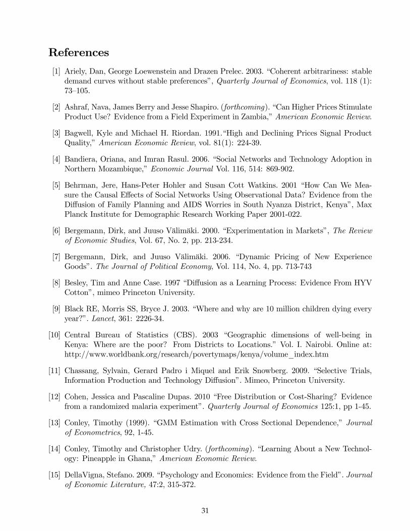
References

[1] Ariely, Dan, George Loewenstein and Drazen Prelec. 2003. �Coherent arbitrariness: stabledemand curves without stable preferences�, Quarterly Journal of Economics, vol. 118 (1):73�105.

[2] Ashraf, Nava, James Berry and Jesse Shapiro. (forthcoming). �Can Higher Prices StimulateProduct Use? Evidence from a Field Experiment in Zambia,�American Economic Review.

[3] Bagwell, Kyle and Michael H. Riordan. 1991.�High and Declining Prices Signal ProductQuality,�American Economic Review, vol. 81(1): 224-39.

[4] Bandiera, Oriana, and Imran Rasul. 2006. �Social Networks and Technology Adoption inNorthern Mozambique,�Economic Journal Vol. 116, 514: 869-902.

[5] Behrman, Jere, Hans-Peter Hohler and Susan Cott Watkins. 2001 �How Can We Mea-sure the Causal E¤ects of Social Networks Using Observational Data? Evidence from theDi¤usion of Family Planning and AIDS Worries in South Nyanza District, Kenya�, MaxPlanck Institute for Demographic Research Working Paper 2001-022.

[6] Bergemann, Dirk, and Juuso Välimäki. 2000. �Experimentation in Markets�, The Reviewof Economic Studies, Vol. 67, No. 2, pp. 213-234.

[7] Bergemann, Dirk, and Juuso Välimäki. 2006. �Dynamic Pricing of New ExperienceGoods�. The Journal of Political Economy, Vol. 114, No. 4, pp. 713-743

[8] Besley, Tim and Anne Case. 1997 �Di¤usion as a Learning Process: Evidence From HYVCotton�, mimeo Princeton University.

[9] Black RE, Morris SS, Bryce J. 2003. �Where and why are 10 million children dying everyyear?�. Lancet, 361: 2226-34.

[10] Central Bureau of Statistics (CBS). 2003 �Geographic dimensions of well-being inKenya: Where are the poor? From Districts to Locations.� Vol. I. Nairobi. Online at:http://www.worldbank.org/research/povertymaps/kenya/volume_index.htm

[11] Chassang, Sylvain, Gerard Padro i Miquel and Erik Snowberg. 2009. �Selective Trials,Information Production and Technology Di¤usion�. Mimeo, Princeton University.

[12] Cohen, Jessica and Pascaline Dupas. 2010 �Free Distribution or Cost-Sharing? Evidencefrom a randomized malaria experiment�. Quarterly Journal of Economics 125:1, pp 1-45.

[13] Conley, Timothy (1999). �GMM Estimation with Cross Sectional Dependence,�Journalof Econometrics, 92, 1-45.

[14] Conley, Timothy and Christopher Udry. (forthcoming). �Learning About a New Technol-ogy: Pineapple in Ghana,�American Economic Review.

[15] DellaVigna, Stefano. 2009. �Psychology and Economics: Evidence from the Field�. Journalof Economic Literature, 47:2, 315-372.

31

[16] Du�o, Esther, Michael Kremer and Jonathan Robinson. 2009. �Nudging Farmers to UseFertilizer: Evidence from Kenya�, mimeo, MIT.

[17] Foster, Andrew and Mark Rosenzweig. 1995 �Learning by Doing and Learning from Oth-ers: Human Capital and Technical Change in Agriculture�, Journal of Political Economy,University of Chicago Press, vol. 103(6), pages 1176-1209.

[18] He¤etz, Ori and Shayo, Moses. 2009. �How Large Are Non-Budget-Constraint E¤ects ofPrices on Demand?�American Economic Journal: Applied Economics vol 1(4):170-99

[19] Jones G, Steketee R, Black RE and the Bellagio Child Survival Study Group. 2003. �Howmany child deaths can we prevent this year?�. Lancet, 362: 65-71.

[20] Kremer, Michael and Edward Miguel. 2007. �The Illusion of Sustainability.�QuarterlyJournal of Economics 122 (3): 1007-1065.

[21] Koszegi, Botond, and Matthew Rabin. 2006. �A Model of Reference-Dependent Prefer-ences,�Quarterly Journal of Economics, 121(4), pp. 1133-1166.

[22] Lengeler, Charles. 2004. �Insecticide-Treated bed nets and curtains for preventing malaria.�Cochrane Dabatase Syst Rev; 2:CF000363.

[23] Manski, Charles. 1993. �Identi�cation of Endogenous Social E¤ects: The Re�ection Prob-lem,�Review of Economic Studies, vol. 60(3), pp.531-42.

[24] Mazar, Nina, Botond Koszegi and Dan Ariely. 2009. �Price-Sensitive Preferences�. Mimeo,UC Berkeley.

[25] McFadden, D. 1999. �Rationality for economists?�, Journal of Risk and Uncertainty, vol.19 (1�3), pp. 73�105.

[26] Moscarini, Giuseppe. 2005.�Job Matching and The Wage Distribution�. Econometrica,Vol. 73, No. 2, pp. 481-516.

[27] Moscarini, Giuseppe, and Lones Smith. 2001. �The Optimal Level of Experimentation�.Econometrica, Vol. 69, No. 6, pp. 1629-1644.

[28] Munshi, Kaivan. 2004. �Social Learning in a Heterogeneous Population: Technology Dif-fusion in the Indian Green Revolution,� Journal of Development Economics 73(1), pp.185-213.

[29] Munshi, Kaivan and Jacque Myaux. 2006. �Social Norms and the Fertility Transition.�Journal of Development Economics 80(1):1-38.

[30] Oster, Emily and Rebecca Thornton. 2009. �Determinants of Technology Adoption: Pri-vate Value and Peer E¤ects in Menstrual Cup Take-Up�. NBER WP 14828.

[31] Sachs, Je¤rey. 2005. The End of Poverty: Economic Possibilities for Our Time, New York:Penguin Press.

32

[32] Simonsohn, Uri, and George Loewenstein. 2006. �Mistake #37: The E¤ect of PreviouslyEncountered Prices on Current Housing Demand �Economic Journal, Vol. 116, No. 508,pp. 175-199.

[33] Simonson, Itamar, and Amos Tversky. 1992. �Choice in context �tradeo¤ contrast andextremeness aversion�, Journal of Marketing Research, vol. 29 (3), pp. 281�95.

[34] Strauss, John, and Duncan Thomas. 1998. �Health, Nutrition, and Economic Develop-ment.�Journal of Economic Literature 36 (2): 766-817.

[35] WHO. 2007. WHO Global Malaria Programme: Position Statement on ITNs.http://www.who.int/malaria/docs/itn/ITNspospaper�nal.pdf

33

1a. Value Function V(p, c*)

1b. Value Function V(pt, c)

Figure 1.

34

Figure 2

Panel A: Share of study households that purchased the LLIN in Phase 1

Panel B: Among households that bought LLIN in Phase 1, share using the net at follow-up

Notes: Data from 1,120 households (Panels A and C), 479 households (Panel B, solid line), 273 households (Panel B, dashed line).The second follow-up was conducted in only 4 of the 6 study areas. Usage is self-reported (see Table 2, cols. 7-9, for results onobserved usage.) The exchange rate at the time of the study was around 65 Ksh to US$ 1 .The number of sampled households in each price group is as follows. FREE: 117 obs; 40-50 Ksh: 173 obs; 60-90 Ksh: 196 obs; 100-120 Ksh: 215 obs; 130-150 Ksh: 199 obs; 190-250 Ksh: 220 obs.

Panel C: Adoption of 1st LLIN, by Phase 1 LLIN price

0.2

.4.6

.81

0 50 100 150 200 250Price of LLIN (in Ksh)

Purchased LLIN with 1st Voucher Quadratic Fit

0.2

.4.6

.81

FREE 40-50 60-90 100-120 130-150 190-250Price Paid (in Ksh)

Using Net at 2-month Follow-up 95% CIUsing Net at 1-yr Follow-up 95% CI

If Purchased 1st LLIN: Using LLIN?

0.2

.4.6

.81

FREE 40-50 60-90 100-120 130-150 190-250Price of LLIN (in Ksh)

Bought LLIN and is Using it at 2-mo Follow-up 95% CIBought LLIN and is Using it at 1-yr Follow-up 95% CI

35

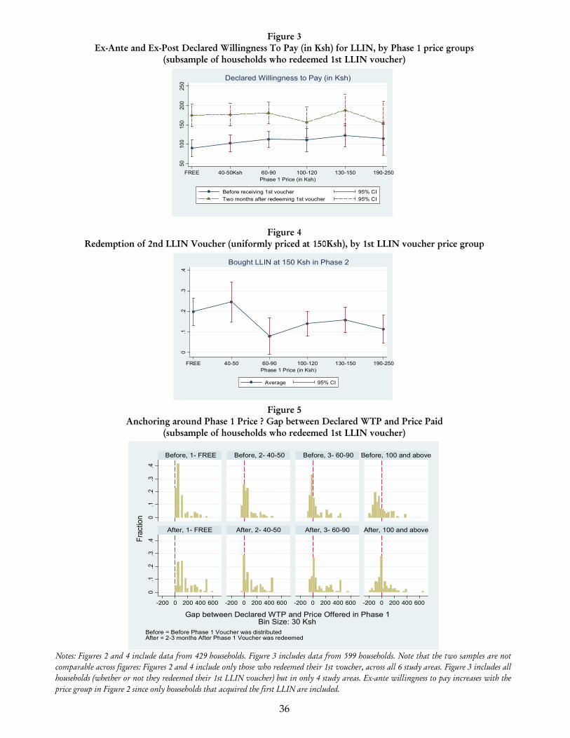
Figure 3Ex-Ante and Ex-Post Declared Willingness To Pay (in Ksh) for LLIN, by Phase 1 price groups

(subsample of households who redeemed 1st LLIN voucher)

Notes: Figures 2 and 4 include data from 429 households. Figure 3 includes data from 599 households. Note that the two samples are notcomparable across figures: Figures 2 and 4 include only those who redeemed their 1st voucher, across all 6 study areas. Figure 3 includes allhouseholds (whether or not they redeemed their 1st LLIN voucher) but in only 4 study areas. Ex-ante willingness to pay increases with theprice group in Figure 2 since only households that acquired the first LLIN are included.

Redemption of 2nd LLIN Voucher (uniformly priced at 150Ksh), by 1st LLIN voucher price groupFigure 4

Figure 5Anchoring around Phase 1 Price ? Gap between Declared WTP and Price Paid

(subsample of households who redeemed 1st LLIN voucher)

0.1

.2.3

.4

FREE 40-50 60-90 100-120 130-150 190-250Phase 1 Price (in Ksh)

Average 95% CI

Bought LLIN at 150 Ksh in Phase 2

5010

015

020

025

0FREE 40-50Ksh 60-90 100-120 130-150 190-250

Phase 1 Price (in Ksh)

Before receiving 1st voucher 95% CITwo months after redeeming 1st voucher 95% CI

Declared Willingness to Pay (in Ksh)

0.1

.2.3

.40

.1.2

.3.4

-200 0 200 400 600 -200 0 200 400 600 -200 0 200 400 600 -200 0 200 400 600

Before, 1- FREE Before, 2- 40-50 Before, 3- 60-90 Before, 100 and above

After, 1- FREE After, 2- 40-50 After, 3- 60-90 After, 100 and above

Frac

tion

Gap between Declared WTP and Price Offered in Phase 1Bin Size: 30 Ksh

Before = Before Phase 1 Voucher was distributedAfter = 2-3 months After Phase 1 Voucher was redeemed

36

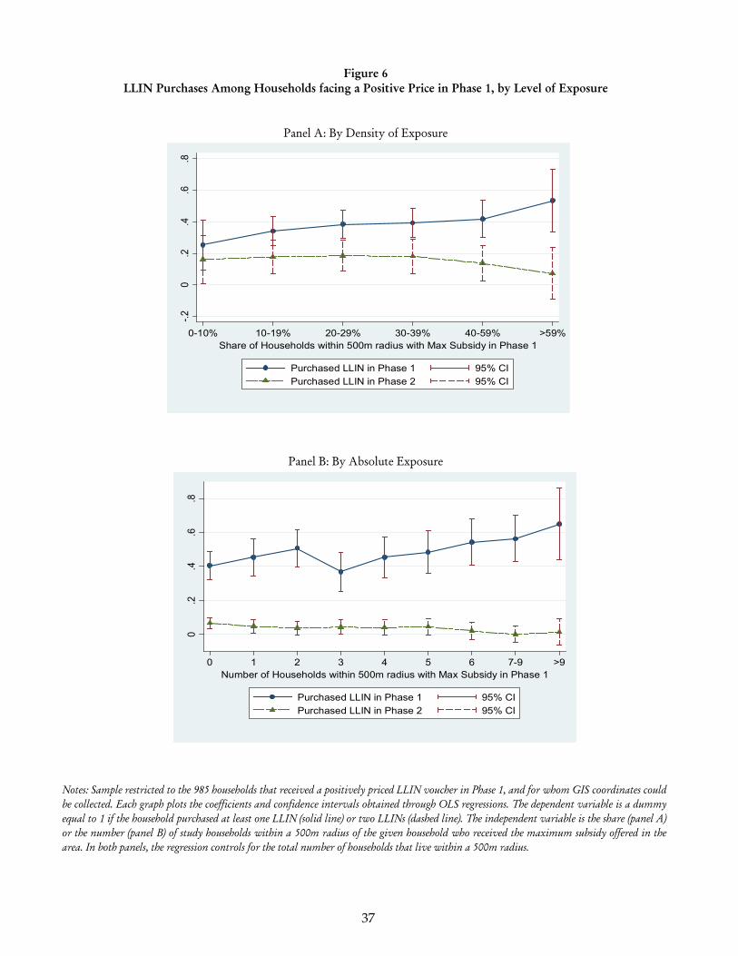
Figure 6LLIN Purchases Among Households facing a Positive Price in Phase 1, by Level of Exposure

Notes: Sample restricted to the 985 households that received a positively priced LLIN voucher in Phase 1, and for whom GIS coordinates couldbe collected. Each graph plots the coefficients and confidence intervals obtained through OLS regressions. The dependent variable is a dummyequal to 1 if the household purchased at least one LLIN (solid line) or two LLINs (dashed line). The independent variable is the share (panel A)or the number (panel B) of study households within a 500m radius of the given household who received the maximum subsidy offered in thearea. In both panels, the regression controls for the total number of households that live within a 500m radius.

Panel A: By Density of Exposure

Panel B: By Absolute Exposure

-.20

.2.4

.6.8

0-10% 10-19% 20-29% 30-39% 40-59% >59%Share of Households within 500m radius with Max Subsidy in Phase 1

Purchased LLIN in Phase 1 95% CIPurchased LLIN in Phase 2 95% CI

0.2

.4.6

.8

0 1 2 3 4 5 6 7-9 >9Number of Households within 500m radius with Max Subsidy in Phase 1

Purchased LLIN in Phase 1 95% CIPurchased LLIN in Phase 2 95% CI

37

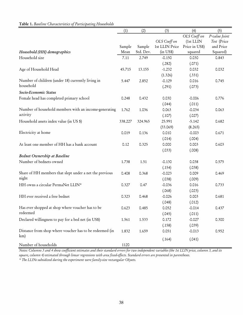
(1) (2) (3) (4) (5)

Household (HH) demographicsSample Mean

Sample Std. Dev.

OLS Coeff on1st LLIN Price

(in US$)

OLS Coeff on(1st LLIN

Price in US$) squared

P-value Joint Test (Price and Price Squared)

Household size 7.11 2.749 -0.150 0.030 0.843(.282) (.071)

Age of Household Head 45.715 13.155 -1.232 0.032 0.032(1.326) (.331)

5.447 2.852 -0.129 0.016 0.745(.291) (.073)

Socio-Economic StatusFemale head has completed primary school 0.248 0.432 0.030 -0.006 0.776

(.044) (.011)1.762 1.036 0.063 -0.034 0.063

(.107) (.027)Household assets index value (in US $) 338.227 324.965 25.991 -5.142 0.682

(33.069) (8.265)Electricity at home 0.019 0.136 0.010 -0.003 0.671

(.014) (.004)At least one member of HH has a bank account 0.12 0.325 0.000 0.003 0.603

(.033) (.008)Bednet Ownership at BaselineNumber of bednets owned 1.738 1.51 -0.130 0.038 0.575

(.154) (.038)0.408 0.368 -0.023 0.009 0.469

(.038) (.009)HH owns a circular PermaNet LLIN* 0.327 0.47 -0.036 0.016 0.733

(.068) (.023)HH ever received a free bednet 0.323 0.468 -0.026 0.003 0.681

(.048) (.012)0.623 0.485 0.052 -0.014 0.437

(.045) (.011)Declared willingness to pay for a bed net (in US$) 1.561 1.533 0.172 -0.027 0.300

(.158) (.039)1.832 1.659 0.051 -0.013 0.952

(.164) (.041)Number of households 1120

Distance from shop where voucher has to be redeemed (in km)

Notes: Columns 3 and 4 show coefficient estimates and their standard errors for two independent variables (the 1st LLIN price, column 3, and its square, column 4) estimated through linear regressions with area fixed-effects. Standard errors are presented in parentheses. * The LLINs subsidized during the experiment were family-size rectangular Olysets.

Table 1. Baseline Characteristics of Participating Households

Number of household members with an income-generating activity

Number of children (under 18) currently living in household

Share of HH members that slept under a net the previous night

Has ever shopped at shop where voucher has to be redeemed

38

(1) (2) (3) (4) (5) (6) (7) (8) (9) (10) (11) (12)

1st LLIN Price in US$ -0.029 -0.043 -0.362(0.042) (0.042) (0.049)***

(1st LLIN Price in US$) squared 0.003 0.006 0.051(0.010) (0.011) (0.012)***

1st LLIN Price = 0 (Free) 0.048 0.061 0.432(0.046) (0.046) (0.055)***

1st LLIN Price ≤ 50 Ksh (High Subsidy) 0.065 0.076 0.361(0.039)* (0.039)* (0.047)***

Experimented with 1st LLIN (instrumented with polynomial in price) 0.123(0.085)

Experimented with 1st LLIN (instrumented with "free" dummy) 0.141(0.107)

Experimented with 1st LLIN (instrumented with "High Subsidy" dummy) 0.212(0.111)*

Household level controls included Yes Yes Yes Yes Yes Yes Yes Yes YesObservations 599 599 599 590 590 590 590 590 590 590 590 590Mean of Dep. Variable in non-free group 0.15 0.15 0.15 0.15 0.27 0.27 0.15 0.15Mean of Dep. Variable in non-"High Subsidy" group 0.14 0.14 0.26 0.14

F-Stat First Stage 51.5 61.3 59.0

Table 3. Effect of 1 st LLIN voucher price on take-up of other product(2) (4) (5)

1st LLIN Price = 0 (Free) 0.066 0.423(0.066) (0.060)***

Experimented with 1st LLIN (instrumented with "1st LLIN Price = 0") 0.154(0.152)

Household level controls included Yes YesObservations 264 275 265Mean of Dep. Variable in non-free group 0.40 0.38 0.40F-Stat First Stage 49.623

Second-Stage (IV): Bought WaterGuard

0.157(0.156)

First-Stage for IV: Experimented with 1st LLIN

0.412(0.056)***

Yes2640.40

Notes: Sample restricted to the 2 areas where WaterGuard vouchers were distributed. "Experimented with 1st LLIN" is a dummy equal to 1 if the household redeemed the 1st LLIN voucher and the net was seen hanging during at least one of the two surprise follow-up visits. Standard errors in parentheses. *Significant at 10%; ** significant at 5%; *** significant at 1%.

54.504

2770.38

0.063(0.062)

2650.40

Bought WaterGuard

(1)

Notes: "Experimented with 1 st LLIN" is a dummy equal to 1 if the household redeemed the 1 st LLIN voucher and the net was seen hanging during at least one of the two surprise follow-up visits.Coefficient estimates obtained using linear regression with area fixed effects. Price of 1st LLIN varies from 0 to US$3.8. Household level controls in columns 3-11 include all 15 variables presented inTable 1. Standard errors in parentheses. *Significant at 10%; ** significant at 5%; *** significant at 1%.

Bought 2nd LLIN

Table 2. Effect of 1 st LLIN price on take-up of 2 nd (uniformly-priced) LLIN

First-Stage (IV): Experimented with 1st LLIN

Second-Stage (IV): Bought 2nd LLIN

(3) (6)

39

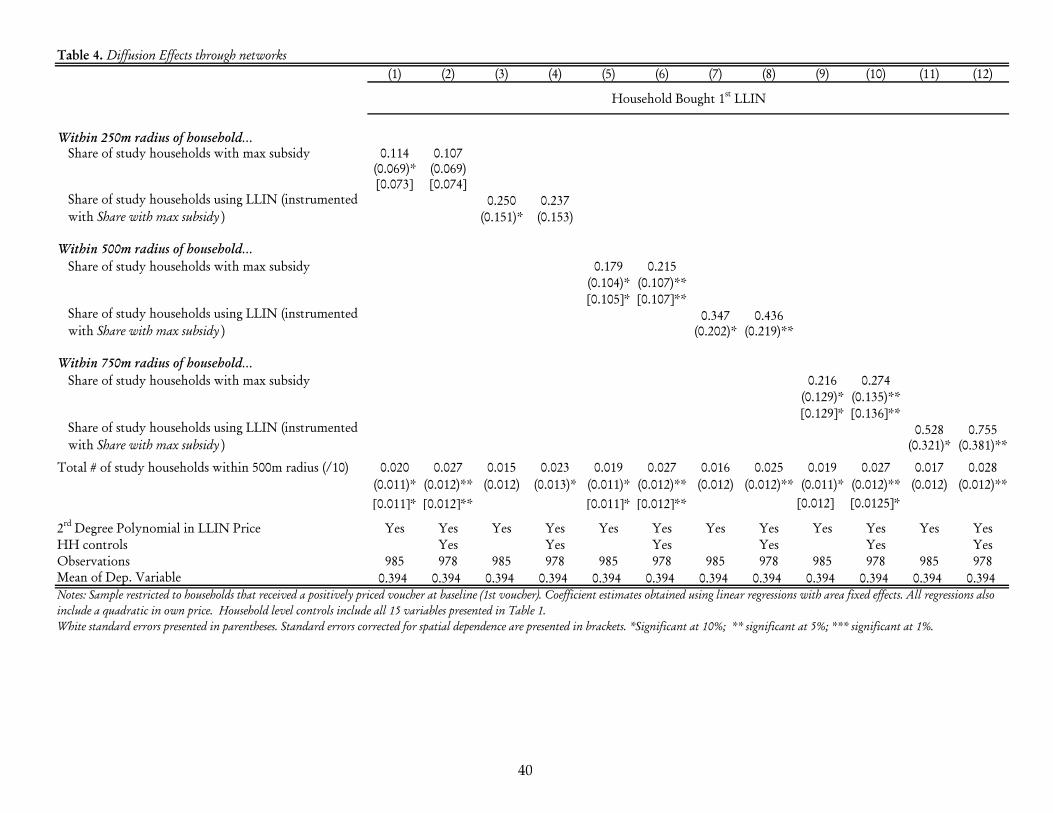
(1) (2) (3) (4) (5) (6) (7) (8) (9) (10) (11) (12)

Within 250m radius of household…Share of study households with max subsidy 0.114 0.107

(0.069)* (0.069)[0.073] [0.074]

0.250 0.237(0.151)* (0.153)

Within 500m radius of household…Share of study households with max subsidy 0.179 0.215

(0.104)* (0.107)**[0.105]* [0.107]**

0.347 0.436(0.202)* (0.219)**

Within 750m radius of household…Share of study households with max subsidy 0.216 0.274

(0.129)* (0.135)**[0.129]* [0.136]**

0.528 0.755(0.321)* (0.381)**

Total # of study households within 500m radius (/10) 0.020 0.027 0.015 0.023 0.019 0.027 0.016 0.025 0.019 0.027 0.017 0.028(0.011)* (0.012)** (0.012) (0.013)* (0.011)* (0.012)** (0.012) (0.012)** (0.011)* (0.012)** (0.012) (0.012)**[0.011]* [0.012]** [0.011]* [0.012]** [0.012] [0.0125]*

2rd Degree Polynomial in LLIN Price Yes Yes Yes Yes Yes Yes Yes Yes Yes Yes Yes YesHH controls Yes Yes Yes Yes Yes YesObservations 985 978 985 978 985 978 985 978 985 978 985 978Mean of Dep. Variable 0.394 0.394 0.394 0.394 0.394 0.394 0.394 0.394 0.394 0.394 0.394 0.394

Household Bought 1st LLIN

Table 4. Diffusion Effects through networks

Notes: Sample restricted to households that received a positively priced voucher at baseline (1st voucher). Coefficient estimates obtained using linear regressions with area fixed effects. All regressions also include a quadratic in own price. Household level controls include all 15 variables presented in Table 1. White standard errors presented in parentheses. Standard errors corrected for spatial dependence are presented in brackets. *Significant at 10%; ** significant at 5%; *** significant at 1%.

Share of study households using LLIN (instrumented with Share with max subsidy )

Share of study households using LLIN (instrumented with Share with max subsidy )

Share of study households using LLIN (instrumented with Share with max subsidy )

40

Figure A1Number of Days needed to Redeem 1st LLIN Voucher, by 1st LLIN voucher price group

Notes: Data from 479 households that redeemed their 1st LLIN voucher.

020

4060

FREE 40-50 60-90 100-120 130-150 190-250Price of LLIN in Phase 1 (in Ksh)

Average 95% CI

41

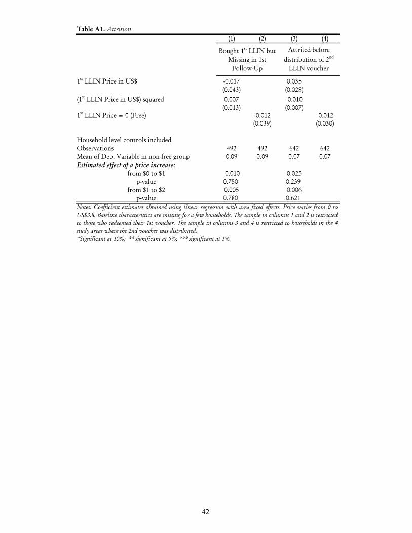
(1) (2) (3) (4)

1st LLIN Price in US$ -0.017 0.035(0.043) (0.028)

(1st LLIN Price in US$) squared 0.007 -0.010(0.013) (0.007)

1st LLIN Price = 0 (Free) -0.012 -0.012(0.039) (0.030)

Household level controls includedObservations 492 492 642 642Mean of Dep. Variable in non-free group 0.09 0.09 0.07 0.07Estimated effect of a price increase:

from $0 to $1 -0.010 0.025p-value 0.750 0.239

from $1 to $2 0.005 0.006p-value 0.780 0.621

Bought 1st LLIN but Missing in 1st

Follow-Up

Attrited before distribution of 2nd

LLIN voucher

Table A1. Attrition

Notes: Coefficient estimates obtained using linear regression with area fixed effects. Price varies from 0 toUS$3.8. Baseline characteristics are missing for a few households. The sample in columns 1 and 2 is restrictedto those who redeemed their 1st voucher. The sample in columns 3 and 4 is restricted to households in the 4study areas where the 2nd voucher was distributed.*Significant at 10%; ** significant at 5%; *** significant at 1%.

42

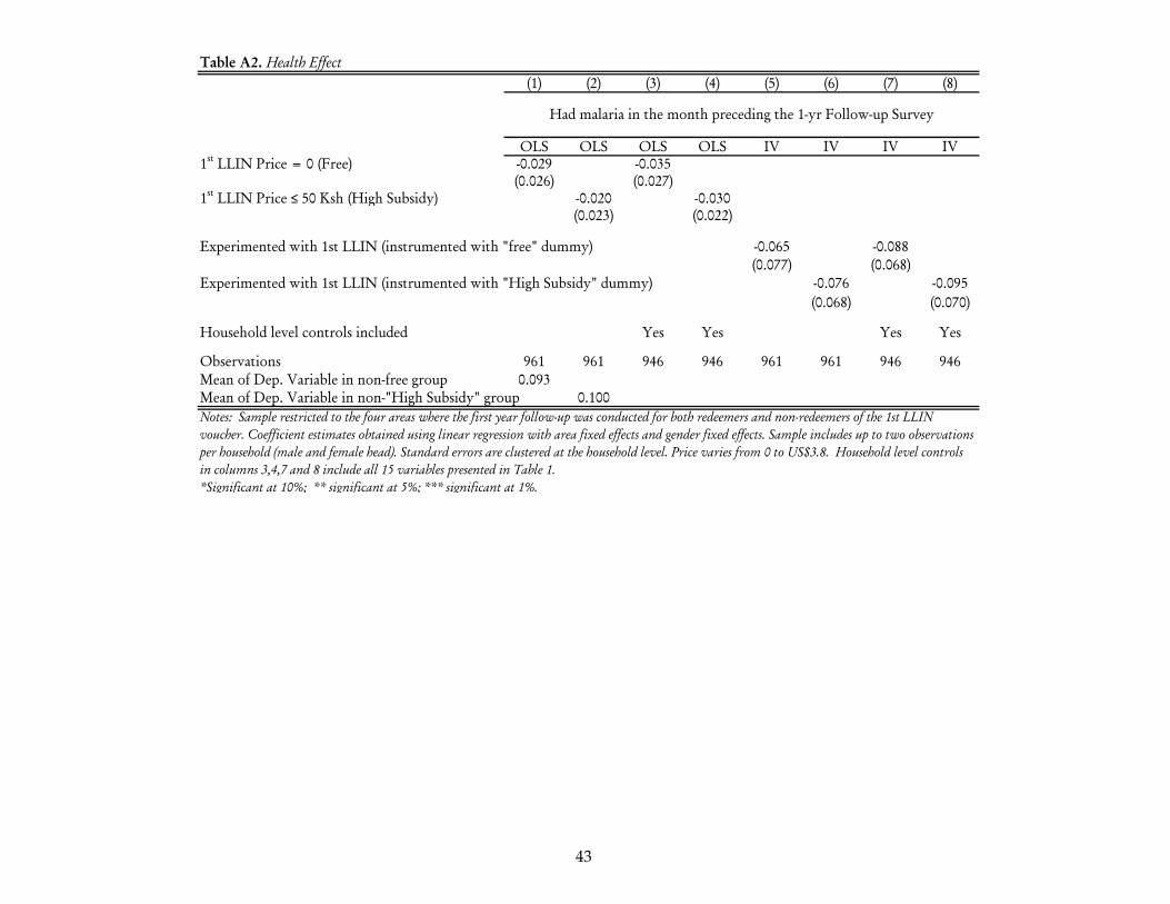
(1) (2) (3) (4) (5) (6) (7) (8)

OLS OLS OLS OLS IV IV IV IV1st LLIN Price = 0 (Free) -0.029 -0.035

(0.026) (0.027)1st LLIN Price ≤ 50 Ksh (High Subsidy) -0.020 -0.030

(0.023) (0.022)

Experimented with 1st LLIN (instrumented with "free" dummy) -0.065 -0.088(0.077) (0.068)

Experimented with 1st LLIN (instrumented with "High Subsidy" dummy) -0.076 -0.095(0.068) (0.070)

Household level controls included Yes Yes Yes Yes

Observations 961 961 946 946 961 961 946 946Mean of Dep. Variable in non-free group 0.093Mean of Dep. Variable in non-"High Subsidy" group 0.100

Table A2. Health Effect

Had malaria in the month preceding the 1-yr Follow-up Survey

Notes: Sample restricted to the four areas where the first year follow-up was conducted for both redeemers and non-redeemers of the 1st LLIN voucher. Coefficient estimates obtained using linear regression with area fixed effects and gender fixed effects. Sample includes up to two observations per household (male and female head). Standard errors are clustered at the household level. Price varies from 0 to US$3.8. Household level controls in columns 3,4,7 and 8 include all 15 variables presented in Table 1. *Significant at 10%; ** significant at 5%; *** significant at 1%.

43

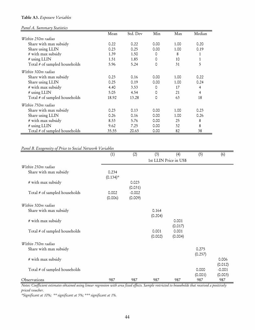
Mean Std. Dev Min Max MedianWithin 250m radius

Share with max subsidy 0.22 0.22 0.00 1.00 0.20Share using LLIN 0.23 0.25 0.00 1.00 0.19# with max subsidy 1.39 1.50 0 8 1# using LLIN 1.51 1.85 0 10 1Total # of sampled households 5.96 5.24 0 31 5

Within 500m radius Share with max subsidy 0.23 0.16 0.00 1.00 0.22Share using LLIN 0.25 0.19 0.00 1.00 0.24# with max subsidy 4.40 3.53 0 17 4# using LLIN 5.05 4.54 0 21 4Total # of sampled households 18.92 13.28 0 63 18

Within 750m radius Share with max subsidy 0.23 0.13 0.00 1.00 0.23Share using LLIN 0.26 0.16 0.00 1.00 0.26# with max subsidy 8.53 5.76 0.00 25 8# using LLIN 9.62 7.25 0.00 32 8Total # of sampled households 35.55 20.65 0.00 82 38

(1) (2) (3) (4) (5) (6)

Within 250m radius Share with max subsidy 0.234

(0.134)*# with max subsidy 0.023

(0.031)Total # of sampled households 0.002 -0.002

(0.006) (0.009)

Within 500m radius Share with max subsidy 0.164

(0.204)# with max subsidy 0.001

(0.017)Total # of sampled households 0.001 0.001

(0.002) (0.004)

Within 750m radius Share with max subsidy 0.275

(0.257)# with max subsidy 0.006

(0.012)Total # of sampled households 0.000 -0.001

(0.001) (0.003)Observations 987 987 987 987 987 987

Panel B. Exogeneity of Price to Social Network Variables

Table A3. Exposure Variables

Panel A. Summary Statistics

1st LLIN Price in US$

Notes: Coefficient estimates obtained using linear regression with area fixed effects. Sample restricted to households that received a positively priced voucher.*Significant at 10%; ** significant at 5%; *** significant at 1%.

44

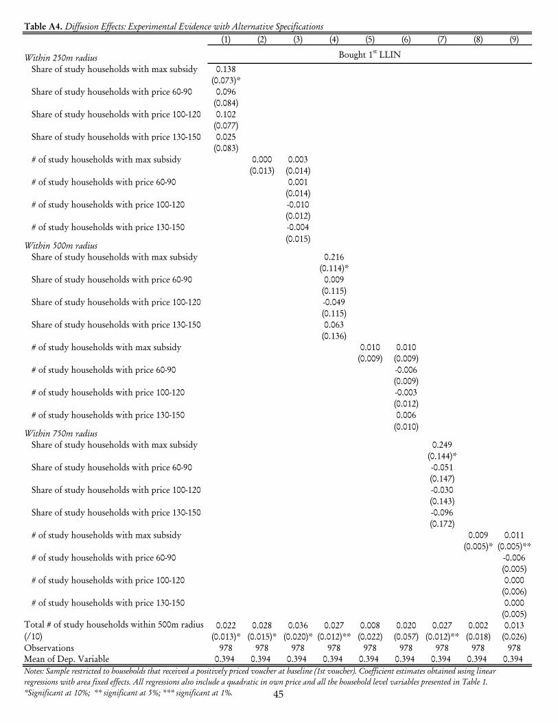
(1) (2) (3) (4) (5) (6) (7) (8) (9)

Within 250m radiusShare of study households with max subsidy 0.138

(0.073)*Share of study households with price 60-90 0.096

(0.084)Share of study households with price 100-120 0.102

(0.077)Share of study households with price 130-150 0.025

(0.083)# of study households with max subsidy 0.000 0.003

(0.013) (0.014)# of study households with price 60-90 0.001

(0.014)# of study households with price 100-120 -0.010

(0.012)# of study households with price 130-150 -0.004

Within 500m radius(0.015)

Share of study households with max subsidy 0.216(0.114)*

Share of study households with price 60-90 0.009(0.115)

Share of study households with price 100-120 -0.049(0.115)

Share of study households with price 130-150 0.063(0.136)

# of study households with max subsidy 0.010 0.010(0.009) (0.009)

# of study households with price 60-90 -0.006(0.009)

# of study households with price 100-120 -0.003(0.012)

# of study households with price 130-150 0.006

Within 750m radius(0.010)

Share of study households with max subsidy 0.249(0.144)*

Share of study households with price 60-90 -0.051(0.147)

Share of study households with price 100-120 -0.030(0.143)

Share of study households with price 130-150 -0.096(0.172)

# of study households with max subsidy 0.009 0.011(0.005)* (0.005)**

# of study households with price 60-90 -0.006(0.005)

# of study households with price 100-120 0.000(0.006)

# of study households with price 130-150 0.000(0.005)

0.022 0.028 0.036 0.027 0.008 0.020 0.027 0.002 0.013(0.013)* (0.015)* (0.020)* (0.012)** (0.022) (0.057) (0.012)** (0.018) (0.026)

Observations 978 978 978 978 978 978 978 978 978Mean of Dep. Variable 0.394 0.394 0.394 0.394 0.394 0.394 0.394 0.394 0.394

Table A4. Diffusion Effects: Experimental Evidence with Alternative Specifications

Notes: Sample restricted to households that received a positively priced voucher at baseline (1st voucher). Coefficient estimates obtained using linear regressions with area fixed effects. All regressions also include a quadratic in own price and all the household level variables presented in Table 1. *Significant at 10%; ** significant at 5%; *** significant at 1%.

Bought 1st LLIN

Total # of study households within 500m radius (/10)

45