exit - the department of mathematics at virginia tech

EXIT CYCLING FOR THE VAN DER POL OSCILLATOR

AND QUASIPOTENTIAL CALCULATIONS

Martin V. Day

Department of Mathematics

Virginia Tech (VPI&SU)

August, 1993

Abstract. We discuss the phenomenon of cycling for noise induced escape to a unstable periodic orbit. The

presence of cycling is shown to follow from qualitative properties of two quasipotential functions. A method of

numerically evaluating these quasipotential functions is described, and applied to the Van der Pol oscillator as an

example. Figures resulting from these calculations reveal that nonconvergent cycling of exit measures does occur

for the Van der Pol example.

x1: IntroductionThe Van der Pol equation

(1.1) �y + �(y2 � 1) _y + y = 0

is a favorite example of a nonlinear system having a unique stable (for � > 0) periodic solution. In the

conventional reduction to a �rst order system, x = (x1; x2) = (y; _y), this becomes

(1.2) _x(t) = b(x(t)) where b(x) =

�x2

��(x21 � 1)x2 � x1

�:

We are going to consider � < 0 (which is equivalent to reversing time for � > 0). This makes (1.2) a system

with a stable critical point at the origin, surrounded by an unstable limit cycle.

The e�ects of adding an asymptotically small random perturbation to such a system have been discussed

in recent work, such as [2] and other references cited there. Speci�cally we compare the solution x(�) of (1.2),with initial condition x(0) = x0, to the solution x�(t) of the following Ito equation:

(1.3) dx�(t) = b(x�(t)) dt + �

1=2d!(t); x

�(0) = x0:

The parameter � > 0 is viewed as the strength of the random perturbation. Our interest is in asymptotic

behavior as � # 0. It can be shown in several ways that x�(t)! x(t) uniformly (in probability) over t in any

�xed time interval [0; T ]. The story is di�erent however when we look at the whole time axis, t 2 [0;1).

Let D be the region enclosed by the limit cycle of (1.2), with @D being the limit cycle itself. For any

x0 2 D the solution x(t) of (1.2) remains forever in D and converges to 0 as t ! 1. In contrast to this,

x�(t) will eventually (with probability 1) wander out to @D, reaching it �rst at some random time � < 1.

A particularly interesting phenomena occurs in the study of the distribution �� of this point x�(�) of �rst

\noise induced" escape to the limit cycle @D:

(1.4) ��(A) = P [x�(�) 2 A]; A � @D:

1991 Mathematics Subject Classi�cation. 60H30, 60H10, 60J70, 60J60.

Key words and phrases. exit problem, limit cycle, quasipotential.

Typeset by AMS-TEX

1

2 MARTIN V. DAY

One might expect �� to converge, as � # 0, to some limiting probability measure on @D. However the

theory suggests that such convergence will hold only in very rare examples. The typical behavior is what

we call periodic cycling. If we could watch the probability measure �� on @D change as � is decreased to

0 we would see it precess or cycle around @D, roughly as if it was being transported along by the ow of

(1.2), with log(��1=2) as the elapsed time. This cycle will (asymptotically) repeat itself each time log(��1=2)

advances by one period of the limit cycle. [2] presents this more precisely, and explains why this will result

in the failure of �� to converge, except in rare examples. One goal of this paper is to o�er numerical evidence

that (nonconvergent) periodic cycling of �� does occur for the Van der Pol system (1.3) in particular.

We will not exhibit cycling of �� through direct simulations or numerical calculations. Rather we numer-

ically evaluate two speci�c functions whose properties are linked to the behavior of �� by the mathematical

theory. These two functions are the quasipotential V (�) (famous from the work of Wentzell and Freidlin

[6]) and the boundary quasipotential W (�). In Section 2 we will brie y introduce these two functions and

present Theorem 1, which explains how the phenomenon of nonconvergent cycling is manifest in qualitative

properties of V and W . Then, in Section 3, we will discuss some �gures which exhibit graphically these

qualitative features, allowing us to invoke Theorem 1 for the example (1.3).

The remainder of the paper concerns the justi�cation of Sections 2 and 3. Section 4 explains the

numerical calculations used to obtain the �gures in Section 3, and the theoretical basis of these calculations.

Section 5 is devoted to proving Theorem 1. Both of these sections depend heavily on detailed understanding

of V and W culled from earlier work, [4] and [3].

The signi�cance of the quasipotential functions (Theorem 1) and our method of evaluating them nu-

merically (Section 4) are not peculiar to the Van der Pol example. Our discussion applies to any example

satisfying the following hypotheses, which are assumed throughout the paper. x�(t) is the (2-dimensional)

solution of

(1.5) dx�(t) = b(x�)dt+ �

1=2�(x�)d!(t); x

�(0) = x0 2 D:(!(t) is a standard 2-dimensional Wiener process and (1.5) is taken in the Ito sense.) The vector �eld b(�)and nonsingular 2�2 matrix function �(�) are smooth on IR2. (We take smooth to mean C1. This is simply

to avoid chasing degrees of di�erentiability through our discussion; Cn for n � 3 would probably be enough.)

The origin is an asymptotically stable critical point of

(1.6) _x(t) = b(x(t));

with all eigenvalues of B = @b

@x(0) having negative real parts. The origin is surrounded by an unstable limit

cycle, with characteristic multiplier m1 > 1. D denotes the region enclosed by the limit cycle, so that @D

is the limit cycle itself. We assume that D contains no other critical points or periodic orbits of (1.6); for

every x(0) 2 D the corresponding solution x(t) of (1.6) has x(t) 2 D for all t > 0 with x(t)! 0 as t! +1.

The perturbed Van der Pol system (1.3) is the particular case with b as in (1.2) and �(�) � I .

The exit measure �� is as de�ned in (1.4). The dependence on x0 is suppressed in the notation because

this dependence does not in uence any of the results described below; the reader may take x0 = 0 in the

de�nition of ��.

It may be worth observing that certain \storage functions" of interest in nonlinear H1 control have

much of the same structure as our quasipotential functions; see [5] and [1]. Thus the numerical approach

described here may also be useful in exploring examples from that context.

x2: Quasipotential Functions and Cycling

The two quasipotential functions, V (�) and W (�), are central to our discussion. Theorem 1 below links

them to the asymptotic behavior of ��. They are de�ned in terms of the \probabilistic action" of Wentzell

and Freidlin. For an absolutely continuous � : [0; T ]! IR2 de�ne

S0T (�) =

Z T

0

L(�; _�) dt

where the Lagrangian L is given by

L(x;v) =1

2(v � b(x))T a(x)�1(v � b(x)):

EXIT CYCLING FOR THE VAN DER POL OSCILLATOR AND QUASIPOTENTIAL CALCULATIONS 3

The matrix a(x) is obtained from the �(x) of (1.5):

a(x) = �(x)�(x)T :

It is therefore smooth, symmetric and positive de�nite. S0T (�) measures (in a sense made precise by large

deviations theory) how unlikely it is for x�(t) to follow the path �(t), for 0 � t � T .

The original quasipotential function is de�ned in �D (the closure of D) by

(2.1) V (x) = inf S0T (�);

where the in�mum is over all T > 0 and absolutely continuous paths � : [0; T ] ! �D with �(0) = 0 and

�(T ) = x. In some sense V (x) measures the probabilistic di�culty of going from x�(0) = 0 to x�(t) = x at

some 0 < t <1 without leaving �D �rst.

The boundary quasipotential function is de�ned in �D by

W (x) = inf S0T (�)

where this time the in�mum is over all T > 0 and absolutely continuous � : [0; T ] ! �D with �(0) = x and

�(T ) 2 @D. It measures the probabilistic di�culty of completing an exit to @D from y.

Properties of V and W have been studied in [4] and [3] respectively. They are both nonnegative

continuous functions in �D. V (0) = 0 with V > 0 in �D n f0g. W = 0 on @D with W > 0 in the interior

of D. More of their structure will be detailed in section 4 in order to explain how we have computed them

numerically. The point here is that nonconvergent cycling of the exit distribution �� can be deduced from

qualitative features of V and W . Theorem 2 and its corollary in Section 5 provide equivalent conditions

which can help identify the presence of these features. Here we use a description in terms of level sets, i.e.

sets of the form

fx 2 D : V (x) = cV g and fx 2 D : W (x) = cW g;for constants cV and cW . We say the level sets of V are coincident with the levels sets of W if for every cVthere is a cW such that the two level sets agree, and likewise for every cW there is a cV .

Theorem 1. If the level sets of V are not coincident with the level sets of W then ��exhibits nonconvergent

cycling as � # 0.The proof of Theorem 1 is discussed in section 5 below. Here we o�er the following rough heuristic

explanation. Consider a level set C of W : C = fW = w0g for some w0 > 0. (If w0 is su�ciently small

C will be close to @D where W is known to be smooth, hence references to dW = [@W@x1

;@W

@x2] below can be

justi�ed.) Since W (y) is constant over y 2 C, the di�culty of completing an exit to @D from y is the same

for all y 2 C. Hence among all possible exit \routes" from 0 to @D the most likely ones are those which

pass through those points y� 2 C which are most easily reached from 0, namely those y� 2 C at which V is

minimal: V (y�) � V (y), all y 2 C. If the V and W level sets do not coincide then the set C� of such y� is a

proper subset of C. It turns out that from a given y 2 C the most likely way to complete an exit to @D is

to follow

(2.2) _x = b(x) � dW (x)T ; x(t0) = y

for roughly log(��1=2) time units and then exit to a nearby boundary point:

x�(�) � x(log(��1=2) + t0):

Now @D is a stable limit cycle for (2.2). So if the y� form a proper subset C� of C then we see the distribution

�� of x�(�) concentrated around x(log(��1=2) + t0) only for those solutions of (2.2) with x(t0) 2 C�. Thesex(log(��1=2) + t0) approximate a proper subset of @D, which cycles or precesses around @D periodically in

log(��1=2), producing the nonconvergent cycling.

4 MARTIN V. DAY

x3: Level Sets for the Van der Pol System

The four accompanying �gures show some of the V and W level sets for the Van der Pol system (1.3)

using two parameter values: � = �1 and � = �2. We discuss the latter of these �rst, since the signi�cant

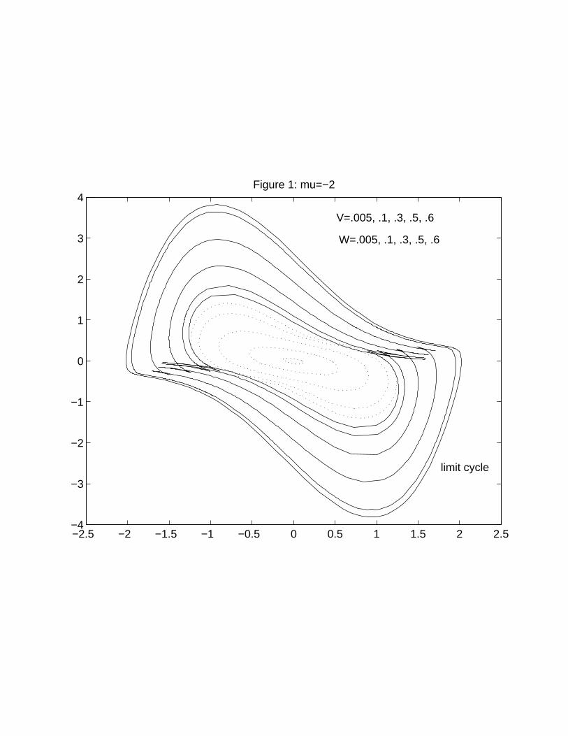
features are more easy to discern in that case. In all �gures the dotted lines indicate V levels, while solid

lines are used for W levels and the limit cycle @D itself.

The Case of � = �2.Figure 1 shows @D (the outer curve) enclosing V andW level sets corresponding to the values indicated

in. The W = :005 set is solid line closest to @D, with the higher W levels being farther into the interior.

V = :005 is the small ellipse near the center; the larger V levels are the concentric dotted curves surrounding

it. Looking carefully, we can see the V = :6 level crossing and recrossing the W = :6 level in both the �rst

and third quadrants.

Figure 2 is an enlarged view showing the crossing of V and W levels in the �rst quadrant more clearly.

Clearly the V = :6 level set does not coincide with aW level, and hence by Theorem 1 nonconvergent cycling

must occur for this example.

The Case of � = �1.Figure 3 shows the limit cycle for � = �1 with an assortment of V and W levels. In this case the V

and W levels seem to be rather close in shape. However di�erences between V = :35 and W = :5 are visible

with close scrutiny.

Figure 4 is an enlargement, using a selection of levels which reveals the noncoincidence more clearly.

W = :5 is close to V = :375 at the top left but crosses V = :35 in the lower right. The V = :2 and W = :75

levels can also be seen to cross. Again we �nd the noncoincidence of the V and W levels to be apparent.

The Fins.

The reader will notice the sharp �n-shaped extrusions attached to some of the W level sets: W � :1

for � = �2, W � :75 for � = �1. Figure 2 a�ords the clearest view. These �ns are not actually part of the

indicated level set, such as fW = :5g in Figure 2, but are an artifact of our computational approach. (See

Section 4.) The presence of these �ns is signi�cant however. The \cross point" where the �n joins the level

set proper is a nonsmooth point for the quasipotential function. The presence of �ns on either the V or W

levels implies the V levels are not coincident with the W levels, as we will explian in Section 5. Hence the

existence of �ns in our pictures is another su�cient condition for nonconvergent cycling.

x4: Computation of Quasipotentials

The numerical calculations used to obtain the graphs of the preceding section will be explained here.

While we make no claims of numerical e�ciency for our approach, it is solidly founded on detailed analysis

of V (�) and W (�), which we summarize below. First we describe some notation and conventions.

The collection of \spatial" points x 2 IR2 is called state space. Many di�erent coordinate systems can

be used to represent points in state space { we will have to deal with a nonstandard one in our discussion

of W below. Until then however we can limit ourselves to the conventional cartesian coordinates x1; x2 and

consider all quantities to be de�ned in terms of coe�cients with respect to them. For purposes of expressions

in which a state x occurs as a factor in a matrix product we will view it as a column matrix: x = [x1; x2]T .

Likewise vectors are taken as columns:

_x =

�_x1_x2

�; b(x) =

�u1(x1; x2)

u2(x1; x2)

�:

The ui(x1; x2) are the speci�c functions which de�ne the dynamical system (1.6). (1.2) gives them expressly

for the Van der Pol system. We write@b

@x=

�@ui

@xj

�

for the matrix of partial derivatives.

The p variables below are taken as rows p = [p1; p2] in matrix product expressions. For such a p and a

vector v = [v1; v2]T , we use hp;vi to denote the scalar

hp;vi = p1v1 + p2v2:

−2.5 −2 −1.5 −1 −0.5 0 0.5 1 1.5 2 2.5−4

−3

−2

−1

0

1

2

3

4Figure 1: mu=−2

limit cycle

V=.005, .1, .3, .5, .6

W=.005, .1, .3, .5, .6

0.4 0.6 0.8 1 1.2 1.4 1.6−0.5

−0.4

−0.3

−0.2

−0.1

0

0.1

0.2

0.3

0.4

0.5Figure 2: mu=−2

limit cycle

W=.5

W=.6

V=.6V=.5

−2.5 −2 −1.5 −1 −0.5 0 0.5 1 1.5 2 2.5−3

−2

−1

0

1

2

3Figure 3: mu=−1

limit cycle

V=.005, .1, .35, .6W=.005, .2, .5, .8

−0.5 0 0.5 1−0.4

−0.2

0

0.2

0.4

0.6

0.8

1

Figure 4: mu=−1

limit cycleW=.2V=.6

W=.5

V=.375V=.35

W=.75V=.1

V=.005


If V (�) is di�erentiable at a point x then dV (x) = [@V (x)

@x1;@V (x)

@x2] denotes the row of partial derivatives. This

is appropriate since dV (x) will often provide the value of p in what follows.

We will work with the Hamiltonian

H(x; p) =1

2hp; a(x)pT i+ hp;b(x)i:

(According to the above conventions a(x)pT de�nes a (column) vector, so that hp; a(x)pT i makes sense.)

H(x; �) is the convex dual of L(x; �):

(4.1) L(x;v) � hp;vi �H(x; p);

with equality for v = Hp(x; p) = b(x) + a(x)pT . The Hamiltonian system associated with H is

(4.2) _xi = Hpi(x; p); _pi = �Hxi

(x; p):

The x equations of (4.2) can be written as

_x = b(x) + a(x)pT :

The p equations are more complicated since they involve second derivatives of b. One can check that for

any solution of (4.2),

(4.3) pi = Lvi(x; _x)

and

(4.4) L(x; _x) =1

2hp; a(x)pT i:

The collection of (x; p) is called phase space. The Hamiltonian system (4.2) is a �rst order system

of di�erential equations in phase space. A solution x(t); p(t) of (4.2) is called a bicharacteristic and its

trajectory in phase space,

f(x(t); p(t)) : t 2 IRg;is called a phase path or phase trajectory. Note that (4.2) is autonomous; a solution can be translated in

time to produce a new solution x(�+ c); p(�+ c) but which traces the same trajectory. We will write ht(�; �)for the ow associated with (4:2). I.e. if x(�); p(�) solves (4:2) then

(x(t); p(t)) = ht(x(0); p(0)):

Note that while vectors in state space are two dimensional, vectors in phase space are four dimensional,

denoted [X1; X2; P1; P2]T below.

Quasipotential.

Some basic properties of the quasipotential V are deduced directly from its de�nition (2.1). We have

already mentioned that V is continuous in �D, V (0) = 0, and V (x) > 0 if x 6= 0. The fact that @D is a

periodic orbit of (1.6) implies that V is constant over @D:

V (x) = v@D for all x 2 @D:

Although the upper bound V � v@D is valid throughout �D, it is possible that V (x) = v@D at some interior

points x as well as on the boundary.

Our computation of V exploits the intimate connection of V with the Hamiltonian system (4.2), as

developed in [4]. For those y 2 D with V (y) < v@D there exists what we call a V -minimizing bicharacteristic

to y: a solution x(�); p(�) to (4.2) which passes through y = x(t0) at some t0 and satis�es

x(t)! 0 as t! �1;

H(x(t); p(t)) � 0

6 MARTIN V. DAY

and

V (y) = V (x(t0)) =

Zt0

�1

1

2hp(t); a(x(t))p(t)T i dt:

In light of (4.4) we can interpret the above as saying x(�) achieves the in�mum de�ning V (y) but using a

semi-in�nite time interval (�1; t0] instead of a bounded [0; T ]. We hasten to point out that x(�); p(�) willnecessarily achieve the minimum to all x(t) for t < t0 as well,

(4.5) V (x(t)) =

Zt

�1

1

2hp; a(x)pT i;

but this can fail if t > t0 is su�ciently large. In fact for each V - minimizing bicharacteristic there exists

� 2 (�1;1] so that x(�); p(�) is minimizing to x(t) for t � � but not for t > � . Moreover V (�) is smooth in

a neighborhood of each of the x(t), t < � and p(t) = dV (x(t)) there, a fact we will use in the next section.

Observe that x = 0, p = 0 is a critical point for (4.2). It turns out that the V -minimizing bicharacteristics

are precisely those lying on the unstable manifold M0 for that critical point. I.e. M0 is the union of the

trajectories of all V -minimizing bicharacteristics. The x(t); p(t) for t > � are still considered part of M0,

even though the minimum to y = x(t) may be achieved by a di�erent ~x(�); ~p(�) to y = ~x(s). (It must be that

p(t) 6= ~p(s), else the two bicharacteristics would only di�er by a translation.)

Another result from [4] says that V is a smooth solution of

H(x; dV (x)) = 0

in some neighborhood of 0. To be explicit we can take this neighborhood to be

N0 = fx 2 D : V (x) < �0g

for a su�ciently small 0 < �0 < v@D. The manifold M0 includes all (x; p) with x 2 N0 and p = dV (x).

Given a V - minimizing bicharacteristic there is a well-de�ned �rst time that x(t) leaves N0:

�0 = infft : x(t) =2 N0g > �1:

It is a fact that

(4.6) both x(t) 2 N0 and p(t) = dV (x(t)) hold if and only if t < �0:

It may be that x(t) returns to N0 at some future time, t > �0, but then p(t) 6= dV (x(t)) and will have ceased

to be V -minimizing, i.e. t > � .

Consider any y 2 D with V (y) < v@D . There exists at least one (possibly many) bicharacteristics from

M0 with x(t) = y (some t). For all of these

V (y) �Z t

�1

1

2hp; a(x)pT i:

Equality will hold for at least one. To �nd the level set fV (x) = cg for a value 0 < c < v@D we can

look at the set of all x(tc) where x(�); p(�) ranges over the bicharacteristics from M0 and tc is determined

by c =R tc�1

12hp; a(x)pT i. This set will include the level set of V , and possibly some extraneous points

coming from those bicharacteristics for which � < tc; i.e. which are on M0 but are not minimizing to x(tc):

V (x(tc)) < c. These extraneous points appear as the \�ns" mentioned in Section 3. (Actually no �ns are

visible on the particular V levels pictured in Section 3. What we observed there were �ns on the W levels;

see below.)

The system (4.2), with

(4.7) _v =1

2hp; a(x)pT i


adjoined can be integrated numerically from an initial point (x0; p0; v0) with x0 2 N0, p0 = dV (x0) and

v0 = V (x0) to produce a bicharacteristic x(�); p(�) from M0, with v(t) = V (x(t)) holding for t < � . The

di�culty is that the only such initial point we know directly is x0 = 0, p0 = dV (0) = 0, which is a stationary

point for (4.2). However the fact that M0 is the unstable manifold of (4.2) allows us to compute its tangent

space at the critical point x = 0, p = 0 and use that to approximate nearby x0; p0 on M0. Calculation of

the tangent space by linearization of (4.2) was carried out in [4]. Let

B =db

dx(0); A = a(0):

For the Van der Pol example in particular,

B =

�0 1

�1 �

�; A = I:

The linearization of (4.2) at x = 0, p = 0 is

d

dt

264X1

X2

P1

P2

375 = �

264X1

X2

P1

P2

375 where � =

�B A

0 �BT

�:

One invariant subspace for � is described by P1 = P2 = 0, within which the eigenvalues of � are just those

of B, which are negative. Another (and the one we want) is described by [X1; X2]T = S[P1; P2]

T where S is

the symmetric 2� 2 matrix solving

(4.8) BS +A+ SBT = 0:

Within this subspace � has the same eigenvalues as �BT , which are positive. This means that the tangent

space to M0 at x = p = 0 is given by �P1

P2

�= S

�1

�X1

X2

�:

We can solve (4.8) explicitly for the Van der Pol example:

S = �� 1�+ �

212

12

1�

�; S

�1 =1

1�2

+ 14

��1�

12

12

�( 1�+ 1

4)

�:

Thus we can describe M0 and V for x � 0 by

(4.9) pT = S

�1x+ o(jxj); V (x) =

1

2xTS�1x+ o(jxj2):

Computation. We begin the computation of level sets of V by choosing a small value 0 < v0 (we used

v0 = :005) and use (4.9) to approximate x and p coordinates of points on M0 corresponding to V (x) = v0.

Given a unit vector

z = [cos(�); sin(�)]T

we take x0 = h � z where h > 0 is chosen so that

v0 =1

2xT

0 S�1x0 =

1

2h2zTS�1z; that is h =

�2v0

zTS�1z

�1=2

:

Then we take pT0 = hS�1z. Doing this for a large selection of � 2 [0; 2�) gives a collection of x0 approximating

the initial level set fV (x) = v0g and the associated p0 = dV (x0) in M0. Each of these provides an initial

point for (4.2) and (4.9).

Next we select a set of desired V -levels: v0 < v1 < v2 < � � � < vn. For each initial point above we

integrate (4.2) and (4.7) numerically, stopping at those times that v(ti) = vi and recording the point x(ti).

Thus for each initial point we generate one (possible) point on each of the level sets fV (x) = vig. These setsof points are then plotted, resulting in the �gures of the preceding section.

The initial points are only approximations to M0, but because M0 is the unstable manifold we expect

solutions of (4.2) close to M0 to converge to the solutions actually on it. In other words we expect the

error in using the linear approximation to M0 to be compensated by the negative eigenvalues of �, at least

initially. We have also checked the sensitivity to this approximation by reducing v0 to compare with a more

accurate approximation. We found negligible di�erences (on the magnitude scale visible in the �gures), thus

supporting our con�dence in the accuracy of the results.

8 MARTIN V. DAY

Boundary Quasipotential.

Most of what has been said about V has an analogue for W ; see [3]. W is continuous in �D, has W = 0

on @D and satis�es

0 < W (x) �W (0) for x 2 D:For any y withW (y) < W (0), the in�mum de�ningW (y) is achieved by someW -minimizing bicharacteristic

from y: a solution x(�); p(�) of (4.2) with x(t1) = y, x(t)! @D as t! +1 (this only means dist(x(t); @D) !0, not that x(t) converges to a point on @D) satisfying H(x(t); p(t)) � 0 and

W (y) =

Z1

t1

1

2hp; a(x)pT i dt:

There will exist �1 � ��< 1 such that x(�); p(�) is W -minimizing from x(t) for all t � �

� but not from

x(t) for t < ��.

The union of the phase trajectories for the W -minimizing bicharacteristics forms a set M@D in phase

space which is the stable manifold associated with the periodic solution of (4.2) consisting of the original

limit cycle x(�) 2 @D of (1.6) with p(�) � 0 adjoined. W is a smooth solution of H(x;�dW (x)) = 0 in a

neighborhood

N@D = fx 2 D : W (x) < �1gof @D. M@D contains the graph of p = �dW (x) for x 2 N@D. For every W -minimizing bicharacteristic,

(4.10) both x(t) 2 N@D and p(t) = �dW (x(t)) hold if and only if �1 < t;

where �1 is the last time x(t) enters N@D:

�1 = supft : x(t) =2 N@Dg < +1:

Our approach to computing a level set fW (x) = cg is analogous to what we did for V . The desired level

set will be contained in the set of all x(tc) where x(�); p(�) range over all the bicharacteristics in the M@D

family and tc is determined by

c =

Z1

tc

1

2hp; a(x)pT i dt:

This set of x(tc) may contain extraneous \�ns" coming from bicharacteristics for which tc precedes the time

�� from which point on x(�) is W -minimizing. (We saw several examples of such �ns in Section 3.) We want

to carry this out numerically by approximating x0; p0 on M@D for which (4.10) holds, and corresponding

w0 =W (x0), and then integrating (4.2) along with

(4.11) _w = �1

2hp; a(x)pT i

backwards in time. We use the tangent space(s) to M@D along @D, p = 0 to approximate (x0; p0) values.

These tangent spaces were described in [3]. However that description was in terms of a special boundary

coordinate system, not the standard cartestian coordinates x1; x2. Hence we have a number of issues of

translation between coordinate systems to work out in order to produce the approximate initial points that

we desire.

The boundary coordinate system from [3] identi�es points near @D using a pair of coordinates denoted

�1; �2. (In [3] xi denoted the boundary coordinates; we have changed to �i since we are using xi for cartesian

coordinates.) @D consists of those points with �1 = 0, so that �2 is a parameter along @D. To be speci�c we

choose �2 to correspond to units of time along the limit cycle: take y�(t) to be the periodic solution of (1.6)

and identify �2 = t. For a given �2 the point with �1 = 0 is just y�(�2). Points with �1 > 0 are interior to D

on the line normal to @D through y�(�2). Let J be the rotation matrix

J =

�0 1

�1 0

�:


then

Jb(y�) =

�u2(y

�)

�u1(y�)�

is an interior normal to D at y� 2 @D. (This assumes y� traverses @D in the clockwise direction, the

clockwise rotation of b points into the interior. For counterclockwise rotation of @D we would negate the

de�nition of J .) The coordinate map (�1; �2) 7! (x1; x2) is given explicitly by

(4.12) (x1; x2) = y�(�2) + �1 � Jb(y�(�2)):

This formula tells us how to calculate the cartesian coordinates of a point from its boundary coordinates.

We will use both x = (x1; x2) and � = (�1; �2) to refer to a common point in state space, choosing between

the x or � notations to emphasize which of the coordinate systems or representations have in mind. For

instance b(�) in (4.15) below is the same vector (in the intrinsic sense) as b(x), but represented di�erently.

We continue to use matrix representations with respect to cartesian coordinates for most formulas of this

section; b = [u1; u2]T and @b

@x= [ @ui

@xj] just as above in our discussion of V . Likewise jbj2 below refers to

(u1)2 + (u2)

2. Even though we are calculating quantities associated with the boundary coordinate system,

we want to be able to carry out the calculations in terms of cartesian representations since that is the form

in which we know b explicitly.

The matrix of partial derivatives (Jacobian) of the coordinate transformation is computed directly from

(4.12):

(4.13)@x

@�=

�@xi

@�j

�= [ Jb j b ] + �1 � [ 0 j J

@b

@xb ] ;

where the terms from b and its derivatives on the right are evaluated at y�(�2). At points y�(�2) on @D

(�1 = 0) we obtain the matrix of partial derivatives of the inverse coordinate map (x1; x2) 7! (�1; �2) by a

simple inversion:

(4.14)@�

@x=

�@�i

@xj

�=

�@xi

@�j

��1

=1

jbj2

24�b

TJ

bT

35 :

The correct ways to translate the representations of state space vectors, p-variables and phase space

vectors are guided by the intrinsic understanding of these quantities, i.e. their appropriate mathematical

meanings apart from any particular coordinate system. What makes the resulting translation formulas

\correct" is that when all quantities ar re-expressed in terms of the new representations, x = (�1; �2),

p = [q1; q2] and H(�; �) = H(�i; qi), then the Hamiltonian system (4.2) takes the same form in the new

expression as it did in the old:_�i = Hqi(�; q); _qi = �H�i(�; q):

The standard intrinsic meaning of a vector at a point is as a �rst order di�erential operator with

evaluation at the point. Suppose x = (x1; x2) and � = (�1; �2) are the two coordinate representations of a

common point. When functions are expressed in terms of the cartesian coordinates f(�) = f(x1; x2) then

the action of b(x) on smooth functions is described by

b(x) = u1(x1; x2)@x1 + u2(x1; x2)@x2 :

The coe�cient functions ui(x1; x2) are expressly known to us from (1.6). However if functions are expressed

in terms of the boundary coordinates f(�) = f(�1; �2) then the same action of b(x) = b(�) is expressed

(4.15) b(�) = �1(�1; �2)@�1 + �2(�1; �2)@�2

using di�erent coe�cient functions �i(�1; �2). It follows then that the correct translation formula is

(4.16)@x

@�

��1

�2

�=

�u1

u2

�:

10 MARTIN V. DAY

Of course the terms are evaluated at the appropriate coordinates �i or xi of a common point.

The construction of our boundary coordinate system implies that the coe�cient functions �i have a

particular asymptotic form near @D. Since @D is f�1 = 0g and b is tangent to @D there, we must have

�1(0; �2) = 0. This means that

�1(�) = �1b1(�) + o(�1)

for �1 � 0, for some function b1(�). Our identi�cation of �2 with time for the motion of (1.6) along @D forces

�2(0; �2) = 1 and so

�2(�) = 1 + �1b2(�) + o(�1)

for some function b2(�). We will need to evaluate b1 on @D in our numerical calculations. To that end we

seek a formula for b1(�) in terms of the cartesian representation of b, valid on @D. Begin with the observation

that

bi(�) = @�1�ij�1=0:

Di�erentiating with respect ot �1 in (4.16) gives

�@�1u1

@�1u2

�=@x

@�

�@�1�1

@�1�2

�+ @�1

@x

@�

��1

�2

�:

Now the left side is

@�1b =@b

@xJb:

Moreover (4.13) implies that

@�1

@x

@�j�1=0 = [ 0 j J

@b

@xb ] :

Using these and our observation that @�1�i = bi on @D, we �nd that

@b

@xJb =

@x

@�

�b1

b2

�+ �2 � J @b

@xb:

Since �2 = 1 on @D, we can solve this to obtain

�b1

b2

�=@�

@x

�@b

@xJ � J

@b

@x

�b:

From (4.14) and JT = �J we lift out the formula

(4.17) b1 =1

jbj2bT

�JT@b

@xJ � @b

@x

�b:

The intrinsic understanding of the p variable is not as a vector but rather as a \covector"; i.e. it is

understood as a linear function acting on vectors. If v is a vector then the action of p on v is the intrinsic

meaning of the h; �; �i notation:p : v 7! hp;vi:

If p = [p1; p2] and v = [v1; v2]T are the representations with respect to cartesian coordinates then we compute

according to the formula

hp;vi = p1v1 + p2v2:

If we switch to the boundary coordinate representation of the same quantities, p = [q1; q2] and v = [�1; �2]T

and want the same quantity to be evaluated using

hp;vi = q1�1 + q2�2:


Then the translation formula (4.16) for vector representations dictates the formula for covector representa-

tions:

[p1; p2]@x

@�= [q1; q2]; or

[p1; p2] = [q1; q2]@�

@x:(4.18)

In particular, our convention of taking dW (x) = [@W@x1

;@W

@x2] as a covector (row matrix), leads to the correct

translation formula (namely the chain rule):

dW (x) = dW (�)@�

@x:

The matrix a(x) acts as a linear map from covectors to vectors, described in coordinates using a matrix

product:

p 7! a(x)pT :

Thus a change in coordinate system will dictate a change in the representation of a(x) as a matrix. If a(x) =

[�ij(x)] is the matrix representation for calculation with respect to cartesian coordinate representations, then

the matrix representation for boundary coordinate representations would have to be

[aij(�)] =@�

@xa(x)(

@�

@x)T :

Our numerical calculations will require evaluation of a11(�) on @D. From the preceding, a11(�) = d�1(x)a(x)d�T

1 (x).

On @D (4.14) tells us that d�1 = � 1jbj2

bT J . Thus at a boundary point (0; �2) = y�(�2) we have the formula

(4.19) a11 =1

jbj4bTJaJ

Tb:

In the Van der Pol example (where a(x) � I) this reduces to a11 =1jbj2

.

Points in phase space now have two di�erent coordinate representations: (xi; pi) or (�i; qi). (4.12) and

(4.18) together provide the coordinate map (�i; qi) 7! (xi; pi). Vectors in phase space have two corresponding

representations:

(4.20) X1@x1 +X2@x2 + P1@p1 + P2@p2 or �1@�1 +�2@�2 +Q1@q1 +Q2@q2 :

The conversion is described by

(4.21)

�X1

X2

�=@x

@�

��1

�2

�;

since @xi

@qj= 0, and

[P1; P2] = [Q1; Q2]@�

@x+ [q1; q2]D;

where

D =Xi

�i@�i@�

@x:

At points (0; �2) 2 @D, with qi = 0 this simpli�es to

(4.22) [P1; P2] = [Q1; Q2]@�

@x

with @�

@xgiven explicitly by (4.14).

12 MARTIN V. DAY

The tangent vectors to M@D at the point y 2 @D, q = 0 were shown in [3] to be given (in boundary

coordinate representation) by

(4.23) Q1 =�1U(y)

�1; Q2 = 0; �i = arbitrary:

The function U is the unique positive continuous function on @D which satis�es

(4.24)d

dtU(y�(t)) = 2b1U � a11;

where b1 and a11 are the functions on @D from (4.17) and (4.19). The terms on the right are evaluated at

y�(t). Note that the periodic solution of (4.24) is unstable in forward time, because if ` is the period of the

limit cycle y�(�) 2 @D thenR`

0b1(y

�) = logm1 > 0 is its Floquet exponent. However in reverse time the

general solution is

u(t) = e�

R0

t2b1(y

�)u(0) +

Z 0

t

e�

Rs

t2b1(y

�)a11(y

�(s)) ds:

Hence it is clear that as t # �1 all solutions converge to

U(y�(t)) =

Z1

t

e�

Rs

12b1(y

�)a11(y

�(s)) ds:

Given that we know the value of U(y) at a boundary point y 2 @D, the tangent vectors (4.23) to M@D at

that point translate to the cartesian representation

(4.25) [P1; P2] = [��1

U(y); 0]

@�

@x=

�1

U(y)jbj2bTJ

and

(4.26)

�X1

X2

�=@x

@�

��1

�2

�= �1 � Jb+�2 � b:

The manifold M@D is, for (�1; �2) near @D, i.e. for �1 � 0, the graph (in phase space) of �dW . In

boundary coordinates this means

qi = @�iW:

The formula (4.23) means that for (�; q) 2M@D with �1 ! 0 and (0; �2) = y 2 @D

q1 = @�1W (�) � �1

U(y)and q2 = @�2W (�) � 0:

This implies

(4.27) W (�) � �21

2U(y):

Computation. The �rst stage of our calculation of W is to locate the limit cycle @D and calculate the

function U de�ned on it. We start with an initial guess x1(0), x2(0) and U(0) and integrate (1.2) along with

(4.28) _U = 2b1(x)U � a11(x)

backwards in time. (4.17) and (4.19) are used to evaluate the coe�cient functions. After a few periods the

solution will have converged to the periodic y�(t) on @D and corresponding values of U(t) = U(y�(t)) along

it. This produces a large collection of y� 2 @D and the corresponding values of U(y�).


Next we take a small w0 > 0 (such as w0 = :005) and for each known value y� with p = 0 move in

the direction speci�ed by tangent vector (4.25), (4.26) with �1 = h > 0 and �2 = 0 to approximate a point

on M@D corresponding to the level set W = w0. Based on the approximation (4.27), select h > 0 so that

w0 =12h2=U(y�):

h =p2w0U(y�):

Now from (4.26) we calculate �X1

X2

�= hJb(y�)

and from (4.25)

[P1; P2] =h

U(y�)jbj2bTJ:

Using these increments from y� 2 @D, p = 0 we obtain approximate coordinate values of the desired the

point on M@D:

(4.29) x0 = y� + hJb(y�); p0 =

h

U(y�)jbj2bTJ:

Finally, suppose we have a set of desired W -levels: w0 < w1 < � � � < wn. We use w0 and each of the

approximate x0; p0 from (4.29) initial values to integrate (4.2) and (4.11) backwards in time, stopping at the

times that w(ti) = wi and recording the point x(ti) as a (possible) point of the level set fW = wig. Theseare then plotted to produce the �gures of the previous section.

x5: Proof of the Sufficiency Theorem

The goal of this �nal section is to prove Theorem 1. The following intermediate result will occupy most

of our e�ort.

Theorem 2. The following are all equivalent:

(1) For any � > 0 there exists 0 < w0 < � so that V is constant over the W level set

fx 2 D : W (x) = w0g:(2) V is smooth in �D.

(3) W is smooth in �D.

(4) V (x) +W (x) is constant in �D.

These equivalents provide a convenient link from Theorem 1 to the study of the cycling phenomenon in [2].

Proof (Theorem 1). Suppose as hypothesized in Theorem 1 that the level sets of V are not coincident with

the level sets of W . Then (4) of Theorem 2 fails and hence so does (1). That means that for all su�ciently

small 0 < w0, V is not constant over the level set

(5.1) fx 2 D : W (x) = w0g:We refer now to Section 4 of [2]. The discussion there concerned @G = f�(x) = �0g where �(x) =

pW (x) and

�0 is su�ciently small but otherwise arbitrary. Hence by taking �0 =pw0 su�ciently small, @G is identi�ed

with the level set in (5.1). The next to last paragraph of Section 4 of [2] explains why nonconvergent cycling

must occur as a consequence of the non-constancy of V over @G.

We note the following corollary to Theorem 2.

Corollary. If any of the conditions (1) { (4) of Theorem 2 are true then the manifolds M0 and M@D

coincide in phase space.

This can be derived from condition (4) without much trouble, but it will come out directly in our proof of

Theorem 2. We believe that M0 = M@D is actually equivalent to the conditions of the theorem, but we

have not proved it. We also conjecture that the coincidence of any one pair of (nonempty) level sets

fW = cW g = fV = cV g

14 MARTIN V. DAY

is su�cient to imply the conditions of the theorem. Since Theorem 2 is adequate for our purposes as it

stands we have not pursued these re�nements.

We also comment that if the conditions (1) { (4) of Theorem 2 hold, then one can argue that each

M0 bicharacteristic is V -minimizing along its full trajectory, i.e. to x(t) for each t, and likewise are W -

minimizing from each x(t). This means that the set of x(tc) that we compute in �nding the levels sets (either

V or W ) contain no extraneous points. I.e. there will be no �ns! Hence the presence of �ns means that (1)

of Theorem 2 fails which, as we have seen, implies nonconvergent cycling of ��.

We turn now to the proof.

Proof (Theorem 2). We will concentrate on the implications (1) ) (2) ) (4) ) (1). Once that is done,

then (2) ) (2)&(4) from which (3) obviously follows. The argument for (3) ) (4) is analogous to that of

(2)) (4), as we will comment below.

Preliminaries There are constructions and notation which we want to develop before coming to grips with

the assertions of the theorem.

Consider the ellipse

E = fx : xTS�1x = �g:For small � > 0, E will be contained in the neighborhood N0 where V is smooth. We claim that if � > 0 is

su�ciently small then E parameterizes the phase trajectories ofM0; i.e. there is a one-to-one correspondence

between the x0 2 E and those phase trajectories x(�); p(�) which satisfy

(5.2) x(t0) = x0 2 E and p(t0) = dV (x0) for some t0:

We know that any phase trajectory satisfying (5.2) for some x0 2 E is on M0. We need to show that each

phase trajectory on M0 satis�es (5.2) for exactly one x0 2 E.Consider the function (x) = x

TS�1x. We know from (4.6) that any bicharacteristic on M0 has

(5.3) p(t) = dV (x(t));

at least until the �rst time �0 that x(t) leaves N0. For all such t < �0

(5.4)d

dt (x) = h2xTS�1;b(x) + a(x)dV T (x)i:

Now we know from (4.9) that

dV (x) = xTS�1 + o(jxj) as jxj � 0:

Using this and

b(x) = Bx+ o(jxj) and a(x) = A+O(jxj)we obtain

d

dt (x) = 2hxTS�1; Bx+ AS

�1xi+ o(jxj2)

= xTS�1AS

�1x+ o(jxj2):

(The last equality is by virtue of (4.8).) The quadratic form occurring here is positive de�nite, so there exists

�0 > 0 so that 0 < (x) � �0 implies both that x 2 N0 and that the right side of (5.4) is positive. Hence for

any bicharacteristic on M0 both (5.3) and (5.4) hold, with (5.4) strictly positive, until after the �rst time

(x(t)) � �0. Since (x(t)) ! 0 as t! �1, there must exist t0 as in (5.2), provided 0 < � < �0. Moreover

for any such t0, (x(t)) is strictly increasing on (�1; t0]. This implies that t0 is unique.

The correspondence (5.2) de�nes a map �0 : N0nf0g ! E, where x0 = �0(x) is the point on E satisfying

(5.2) for the phase trajectory passing through the point x, p = dV (x) onM0. �0 can be shown to be smooth,

using the implicit function theorem.

We want to establish a similar parameterization of M@D by a level set

C = fx 2 D : W (x) = w0g:


Take any w0 < �1, where �1 is as in the de�nition of N@D. Suppose x(�); p(�) is a bicharacteristic on M@D.

From (4.10) the set of t for which

x(t) 2 N@D; and p(t) = �dW (x(t))

is the interval �1 < t, where �1 is the smallest time at which W (x(�1)) � �1. For t in this interval W (x(t))

is strictly decreasing:

(5.5)d

dtW (x) =

1

2hp; a(x)pT i < 0:

Hence there exists a unique x1 = x(t1) such that W (x1) = w0, that is

(5.6) x(t1) 2 C and p(t1) = �dW (x(t1)) for some t1:

Conversely we know that if (5.6) holds for some x1 2 C then the phase path is on M@D. This shows that

there is a one-to-one correspondence between x1 2 C and the phase trajectories onM@D, described by (5.6).

Moreover the map �1 : N@D n @D ! C which takes x to x1 = �1(x) satisfying (5.6) for the phase trajectory

through x, p = �dW (x) is smooth.

(1) implies (2) We assume that V is constant over C with w0 su�ciently small to satisfy the preceding.

Note this constant must be V jC = v@D � w0. Indeed since there exist paths � from C to @D with S0T (�)

arbitrarily close to w0 we must have v@D � V jC + w0. On the other hand if v@D < V jC + w0 then there

would exist a � from 0 to @D with S0T (�) < V jC + w0. � must pass through C at some t 2 (0; T ). Since

S0t(�) � V (�(t)) = V jC we would have

V jC + w0 > S0T (�)

= S0t(�) + StT (�)

� V jC + StT (�);

which implies StT (�) < w0. This is impossible since as a path from �(t) 2 C to �(T ) 2 @D we must have

StT (�) � w0.

Consider any x1 2 C. Since V (x1) < v@D there exists a V - minimizing bicharacteristic x(�); p(�) to

x1 = x(t1). As a V - minimizer it must belong to the M0 family. We claim that it must also satisfy (5.6),

which will show that the V -minimizer to x1 is unique and belongs to the M@D family as well. Let t0 be as

in (5.5) and let x0 = x(t0). Then x(�) must achieve the minimum of

Zt1

t0

L(�; _�) dt

over all absolutely continuous � on [t0; t1] with �(t0) = x0 and �(t1) 2 C. Indeed if there were such a �

with a smaller value ofR t1t0L than x(�), then by concatenating it with x(�) on (�1; t0] we would get a path

from 0 to a point on C with a smaller value of V than V (x1). This is not possible since V is assumed

constant over C. The transversality necessary condition for x(�) to solve this minimization problem implies

that p(t1) = Lv(x(t1); _x(t1)) is normal to C, i.e.

p(t1) = c � dW (x1) for some c 6= 0:

But we also know that both H(x(t1); p(t1)) = 0 and H(x1;�dW (x1)) = 0 hold. Since

0 = H(x; c � dW (x))

= c2hdW (x); a(x)dW T (x)i � chdW (x);b(x)i;

there is at most one nonzero solution c. We conclude that c = �1 and so p(t1) = �dW (x(t1). Hence (5.6)

is indeed satis�ed.

16 MARTIN V. DAY

What we have shown is that for each x1 2 C there is a unique x0 2 E such the phase paths satisfying

(5.2) and (5.6) coincide. Moreover this phase path is the unique V -minimizer to x1. We denote the map

x0 7! x1 so de�ned by : C ! E: x0 = (x1). What we have said so far implies that M@D � M0. We

intend to show that is surjective, which will mean that M@D = M0 (establishing the corollary stated

above).

We claim that is continuous, and is an open map (i.e. it maps open subsets of C to open subsets of

E.) Consider x1 2 C and x0 = (x1) 2 E with x0 = x(t0), x1 = x(t1) along a common bicharacteristic

satisfying (5.2) and (5.6). Let T = t1 � t0. Observe that (x) = �0 � h�T (x;�dW (x)), at least for x 2 C

su�ciently close to x1. This is because both sides produce a point on the same phase trajectory satisfying

(5.2). By uniqueness they must agree. This shows that is smooth. Likewise ~ = �1 �hT (x; dV (x)) de�nesa smooth function from a neighborhood of x0 in E to C. Moreover ~�(x) = x for all x 2 C su�ciently close

to x1, because both sides are on the same phase trajectory and satisfy (5.6) and hence must agree. It follows

from this that has nonvanishing Jacobian at x1 2 E. (This Jacobian can be considered with respect to

any convenient coordinate systems de�ned in neighborhoods of x0 on E and x1 on C.) Since x1 2 E was

arbitrary, standard open mapping results now apply to tell us that is indeed an open mapping.

Since C is compact and is continuous, (C) � E is closed. Since is open, and C is an open subset

of itself, (C) is also open in E. But the ellipse E is connected, so we conclude that E = (C). This

completes our demonstration that M0 =M@D, with the identi�cation provided by via (5.2) and (5.6).

We are now in position to establish 2. Consider any y 2 D. We can choose w0 in the de�nition of

C above so that 0 < w0 < W (y). It follows that V (y) � V jC < v@D , so there exists a V -minimizing

bicharacteristic x(�); p(�) to x(s) = y. As a V -minimizer this must be a phase path from the M0 family.

But since M0 =M@D it also belongs to the M@D family, and is the V -minimizer to some x(t1) = x1 2 C.Since W (y) = W (x(s)) > w0 = W (x(t1)) we must have s < t1. Indeed, (5.6) implies W (x(t)) � W (x(t1))

for all t1 � t. Since x(�) is a V - minimizer to x(t1), V is smooth in a neighborhood of each x(t) with

t < t1. In particular V is smooth in a neighborhood of y = x(s). For y su�ciently near @D we know that

dV (y) = p(s) = �dW (y), since the V - minimizer to y and the W -minimizer from y are the same. Hence the

smoothness of W up to and on @D implies the same for V . This completes the proof of 2.

(2) implies (4) We know V � v@D , with equality on @D. We also know from [4] that

(5.7) H(x; dV (x)) = 0

in 0 = fV < v@Dg. By continuity (5.7) extends to the closure �0. Any point in D n �0 is interior to the set

of x with V (x) = v@D, and so has dV (x) = 0, for which (5.7) is also satis�ed. Hence (5.7) holds in all of D.

We claim that V (x) < v@D for all interior points x 2 D. Otherwise V would have an interior maximum,

and so dV (x0) = 0 at an interior point x0 2 D. We will show that this is not possible. Now (5.7) implies,

by the usual method of characteristics, that the solution x(�) of_x = Hp(x; dV (x)); x(0) = x0

together with p(�) de�ned by

p(t) = dV (x(t))

is a solution of the Hamiltonian system (4.2), with initial conditions x(0) = x0 and p(0) = dV (x0) = 0.

On the other hand p(t) � 0 and the solution of (1.6) with x(0) = x0 also solve (4.2) with the same initial

conditions. Hence both solutions must coincide:

p(t) = dV (x(t)) � 0;

and x(t) ! 0, because of our hypotheses on (1.6). But this would imply V is constant along x(t) so that

0 = V (0) = V (x0) = v@D > 0, a contradiction. Hence it must be that V (x) < v@D at all interior points of

D, as claimed.

The function

(x) = v@D � V (x)

is a smooth solution of

(5.8) H(x;�d (x)) = 0


in �D which is 0 on @D and positive in D. The following \veri�cation argument" will show that = W .

Consider any absolutely continuous � : [0; T ] ! �D with �(0) = x0 and �(T ) 2 @D. Using (4.1) with

p = �d (�) we �ndL(�; _�) � h�d ; _�i �H(�;�d (�)) = � d

dt (�):

Therefore ZT

0

L(�; _�) � (�(0)) � (�(T )) = (x0);

showing that W (x0) � (x0). If we use the solution x(�) of

_x = Hp(x;�d (x)); x(0) = x0

in place of �(�) above then equality holds when we invoke (4.1):

d

dt (x) = �L(x; _x):

Using as a Lyapunov function it follows that x(t)! @D and (x(t)) ! 0 as t!1. Taking T !1 in

ZT

0

L(x; _x) = (x0)� (x(T )):

we conclude that W (x0) � (x0). Thus W (�) � (�) � v@D � V (�), which is to say

V (�) +W (�) � v@D in �D:

We comment that the proof of (3) ) (4) is analogous: (x) = W (0) �W (x) is a smooth solution of

H(x; d (x)) = 0 which is nonnegative in D and 0 at the origin. (Lemma 1 of [RP] is also applicable.)

(4) implies (1) This is trivial; (4) implies that V is constant over a given set if and only if W is.

References

1. J. A. Ball and J. W. Helton, Viscosity solutions of Hamilton-Jacobi equations arising in nonlinear H1-control (Summary),

J. Math. Systems Estimation and Control 6 (1996), 109{112.

2. M. V. Day, Cycling and skewing of exit measures for planar systems, Stochastics 48 (1994), 227{247.

3. , Regularity of boundary quasipotentials for planar systems, Appl. Math. Optim. 30 (1993), 79{101.

4. M. V. Day and T. A. Darden, Some regularity results on the Ventcel-Freidlen quasi-potential function, Appl. Math. Optim.

13 (1985), 259{282.

5. A. J. van der Schaft,, On a state space approach to nonlinear H1 control,, Systems and Control Letters 16 (1991), 1{8.

6. M. I. Freidlin and A. D. Wentzell, Small Random Perturbations of Dynamical Systems, Springer-Verlag, New York, 1984.

Running Head : Cycling and Quasipotentials

Department of Mathematics, Virginia Tech, Blacksburg, VA 24061-0123; [email protected]

exit - the department of mathematics at virginia tech

Documents