Existence and Stability of Traveling Pulses in a

Reaction-Diffusion-Mechanics System

Matt Holzer∗, Arjen Doelman†, Tasso J. Kaper‡

July 5, 2012

Abstract

In this article, we analyze traveling waves in a reaction-diffusion-mechanics (RDM) system. Thesystem consists of a modified FitzHugh-Nagumo equation, also known as the Aliev-Panfilov model,coupled bidirectionally with an elasticity equation for a deformable medium. In one direction, contractionand expansion of the elastic medium decreases and increases, respectively, the ionic currents and alsoalters the diffusivity. In the other direction, the dynamics of the R-D components directly influencethe deformation of the medium. We demonstrate the existence of traveling waves on the real line usinggeometric singular perturbation theory. We also establish the linear stability of these traveling wavesusing the theory of exponential dichotomies.

AMS(MOS) numbers: 35K57, 74H20, 35C07, 35P15Keywords: traveling waves, reaction-diffusion-mechanics equations, waves in deformable media, geometricsingular perturbation theory, spectral stability, exponential dichotomies

1 Introduction

Traveling waves in reaction-diffusion equations have been studied extensively in many areas of science andtechnology, see for example [22, 35, 36]. A prototypical example in neuroscience is the FitzHugh-Nagumo(FHN) equation, see [20]. This PDE models the transmembrane voltage for nerve cells and the dynamicsof a recovery variable. Traveling waves in the FHN equation represent the propagation of action potentialsalong nerve cells. Fundamental characteristics of these traveling waves in FHN, such as their profiles, speeds,decay rates, and stability properties, are by now well understood. Initial studies employed piece-wise linearmodels, [26, 32]. Existence and stability for the full smooth FHN PDE was established in [4, 15, 17].

One of the interesting new directions in which the FitzHugh-Nagumo type modeling has been takenrecently involves the bidirectional coupling of a reaction-diffusion equation and a mechanics equation thatgoverns the deformations of the medium in which the action potential propagate. Such models are referred toas reaction-diffusion-mechanics (RDM) models. They are a natural next step for modeling wave propagationin certain deformable media using continuum models, and they present novel mathematical challenges.

A prototype example is the RDM model developed by Panfilov, Keldermann, and Nash [27, 30]. Theymodeled the mechanical deformation of a 2-D patch of heart muscle fiber using equations for elastic media.Then, they bidirectionally coupled this elasticity equation to a modified FitzHugh-Nagumo equation. In onedirection, the stretching and contraction of the heart muscle directly change the magnitudes of the currentand diffusivity in the voltage equation, because the deformation directly alters the number of ion channelsthat are open or closed. In the other direction, variations in the magnitude of the current result in changesin the deformation of the medium. This model was motivated by experiments, including those in [21, 24].

The coupled RDM system with two-dimensional elasticity equations involves a second-order PDE coupledto the reaction-diffusion equations. Hence, it is difficult to analyze directly. However, locally, the heart muscle

∗School of Mathematics, University of Minnesota, 127 Vincent Hall, 206 Church St. SE, Minneapolis MN 55455, USA†Mathematisch Instituut, Universiteit Leiden, Postbus 9512, 2300 RA Leiden, the Netherlands‡Department of Mathematics and Statistics & Center for BioDynamics Boston University, 111 Cummington Street, Boston,

MA 02215, USA

1

tissue consists, to a good approximation, of parallel muscle fibers. Therefore, the dominant deformations areone-dimensional, corresponding to the stretch and contraction of individual fibers. While this approximationneglects important effects created by the coupling between adjacent fibers, it will be useful as a first step inthe analysis of the full two-dimensional model. In addition, the analysis of this one-dimensional model onthe real line will be a building block for the treatment of the coupled RDM system on a periodic domain.

In this article, we study the following RDM model on the real line,

∂u

∂t=

1

F

∂

∂X

(1

F

∂u

∂X

)− ku(u− a)(u− 1)− uw

∂w

∂t= ε(ku− w)

F (X, t) =1

2+M

4c1+

1

2

√(1 +

M

2c1)2 − 2

c1w(X, t). (1.1)

Here, the R-D components u and w are the same as in the modified FitzHugh-Nagumo equation studiedin [30]. Namely, u represents voltage and w a recovery variable. The key parameters are a, which measuresthe degree of excitability in the medium and k, a rate constant. The coupling between u and w is nonlinear,exactly as in the Aliev-Panfilov modification of the classical FHN equation, see [1], and this contrasts withthe linear coupling in the classical FHN equation. In addition, the separation of time scales between the uand w dynamics is modeled by the asymptotically small parameter ε. See Section 2.1.

The mechanical component, modeled by the deformation F (X, t), is derived from the equation for anelastic medium using a Piola-Kirchhoff type stress tensor under the assumption that the medium is hypere-lastic. It is assumed that the stress is a linear combination of active and passive components and that theactive stress is dependent only on the recovery variable w. The parameter c1 is a measure of the internalenergy of the deformable medium and it scales the relative importance of the passive and active stresses.The medium is assumed to be in mechanical equilibrium, which for one-dimensional objects is equivalent toconstant stress throughout. The constant M is this stress, measured in material coordinates. Application ofthese conditions simplifies the 1-D elastic medium equations to a single formula for the deformation F , asin (1.1). See Section 2.2.

In system (1.1), the bidirectional coupling between the R-D components u and w and mechanical com-ponent F is modeled by the w dependence in the formula for the deformation F and the dependence ofthe diffusivity in the voltage equation on the deformation F . In addition, it is possible to incorporate astretch activated current, ISAC into (1.1). However, the incorporation of stretch activated currents is moreapplicable to bounded domains (for reasons that will be explained in section 2.4) so we will focus on the caseISAC = 0.

The first main result of this article is the existence of traveling waves in the RDM system (1.1) onthe real line. See Theorem 1 in Section 3 below. These traveling waves are similar to the fast pulses ofthe classical FitzHugh-Nagumo equation, consisting of fronts and backs concatenated together, interspersedwith quiescent and active phases. We focus here on the regime in which the back jumps from the knee ofthe active branch, rather than from below the knee, where the knee is the nonhyperbolic local maximum ofthe right (active) branch of the cubic nullcline in (1.1). Pulses of this type are relevant for cardiac modelsand also present mathematical challenges due to the non-hyperbolicity of the knee. The existence analysisconsists of constructing the appropriate singular homoclinic solution and showing that it lies in the transverseintersection of the appropriate center-unstable and center-stable manifolds of the asymptotic state. Centermanifold theory and geometric desingularization near the knee are also needed to carry out this construction.This aspect of the work is similar to the approach developed recently in [3].

The second main result is the spectral stability analysis of the traveling waves in the RDM model (1.1).We determine the parameter regime in which the traveling waves are stable using the method of exponentialdichotomies. See Theorem 3 and its proof in Section 4–6. Exponential dichotomies are shown to exist overthe individual segments of the singular homoclinic solution. The stable and unstable subspaces are trackedover the entire pulse using the estimates from these dichotomies along each segment, and roughness of thedichotomies is used to bootstrap up to the full system with 0 < ε 1. We note that this approach differsfundamentally from that used in [17] for the classical FHN equation and from that used in [3] for a cardiacmodel. Exponential dichotomies have been used to establish spectral stability in other partial differential

2

equations, see for example, Section 3.2 in [34]. We remark that the results about the spectrum of thelinearized operator in this article can also be used to obtain semi-group results, especially concerning thespectrum of the operator obtained by exponentiating this linear operator. We refer the reader to [2] , as wellas to the more recent analysis in [14, 33], for general results.

Besides being of interest in their own rights for the RDM model (1.1), the existence and stability analyseswe present are essential building blocks for other RDM modeling in this direction. The RDM model developedin Section 2 also applies to 1-D models on finite domains and on periodic domains. The existence analysisand the stability analysis (via exponential dichotomies) are well-suited for spatially-periodic problems. Inaddition, we hope that the methods developed here may find application in other RDM systems. One suchsystem involves mechanically induced oscillations in a gel [39]. In addition, there are a number of phenomenaassociated to pulse propagation, such as blocking and propagation failure, and it would be of interest to studythem also in this RDM system.

The article is organized as follows. In section 2, the RDM model of Panfilov, Keldermann and Nash isdeveloped in one dimension. In section 3, we establish the existence of a traveling pulse. Then in sections4-6 the spectral stability of this pulse is established.

2 Derivation of the RDM Model

In this section, we build up the reaction-diffusion-mechanics (RDM) model in one dimension. We follow veryclosely the work of Panfilov, Keldermann, and Nash [30] who developed the model in higher dimensions.

2.1 Equations for electrical activity

We consider a modified Fitz-Hugh Nagumo model in one spatial dimension. Introduced in [1], this modifiedFitz-Hugh Nagumo equation models the excitation and propagation of electric currents in cardiac tissue.The two state variables are u, which represents the transmembrane potential and w, a recovery variable.They are governed by the following reaction-diffusion equations:

ut = Duxx − f(u,w)

wt = ε(u)(ku− w), (2.1)

with f(u,w) = ku(u − a)(u − 1) + uw, where D, k and a are parameters, and ε(u) is a step function withε(u) = 1 if u < .05 and ε(u) = .1 otherwise. This step function is included to capture the time scale ofrecovery. The domain can be taken to be the finite interval [0, L], a ring or the infinite real line R.

2.2 Mechanical Deformation

In cardiac cells, changes in transmembrane potential lead to contraction of the cardiac tissue. Following[27, 30], we use finite deformation elasticity theory to develop a mechanical model of deformation to coupleto the excitable model given by (2.1). For a reference on finite deformation elasticity, see [25, 16] amongothers. In one dimension many things simplify. In particular, all quantities are scalar functions instead oftensors. Our approach is to consider the one dimensional medium as being embedded in a three dimensionalmedium, but require the medium to be undeformable in all directions other than the embedded one.

We begin with a set of reference (material) coordinates, X, which at some time t have deformed to a newposition given by

x = φ(X, t).

The deformation of the material at time t is represented by F = ∂x∂X . In deformed coordinates, the stress, or

force per unit area, at a point x is given by T (x). It is preferable to work in terms of material coordinates,so we define a second stress tensor, T (X), that measures the stress in terms of force per unit undeformedarea. This tensor is known as the second Piola-Kirchhoff stress tensor and is related to T by FT = T . Forany arbitrary deformation, conservation of momentum implies that the tissue is in equilibrium if

∂

∂XFT = 0. (2.2)

3

In deformed coordinates, the equilibrium condition is given by ∂T∂x = 0. Postulating an internal energy of

the form W (F ) = c1(F − 1)2, we may derive via conservation of energy that the stress is given by

T (X, t) =1

F

∂W

∂F= 2c1

F − 1

F. (2.3)

This is known as the passive stress. Combining the conditions (2.2) and (2.3), we arrive at the governingequation for the deformation in the absence of electrical coupling,

∂F

∂X= 0.

To couple the deformation to the potential u, we follow [27, 30] and introduce an active stress, Ta(X, t),which evolves in time according to

∂Ta∂t

= ε(u)(kTu− Ta),

where kT is a parameter. The active stress sums with the passive stress (2.3) to yield the total stress,

T (X, t) = 2c1F − 1

F+TaF 2

.

The equilibrium condition (2.2) is used to derive an expression for the evolution of the deformation F (X, t).In particular, we have that

∂

∂X

(2c1(F − 1) +

TaF

)= 0.

One way in which to interpret this condition is that the product of the deformation and the second Piola-Kirchhoff stress is equal to a constant in X. In other words, we have

2c1(F − 1) +TaF

= M,

for some M which can depend on t but not on X. We apply the equilibrium condition (2.2) and solve forthe deformation as

F (X, t) =1

2+M

4c1+

1

2

√(1 +

M

2c1)2 − 2

c1Ta(X, t). (2.4)

This formula for the deformation F is almost the final form that is stated in the RDM model (1.1).

Remark 1. Note that if Ta >c12 (1 + M

2c1)2, the mechanical model no longer possesses static equilibrium and

(2.4) is no longer valid. To extend the model to the regime of large Ta, a PDE for the temporal evolutionof the displacement would have to be included representing the conservation of momentum. Since we areinterested in traveling pulses with at most small perturbations, in this article we will focus on the case whenthe mechanical model is in equilibrium and the deformation can be expressed explicitly as in (2.4).

Remark 2. The spatial constant M is related to the boundary conditions placed upon the mechanical medium.Natural boundary conditions for mechanical models involve geometric constraints, surface tractions or somecombination of the two. Thus, they are conditions placed upon either the displacement φ or the stress T .In one spatial dimension, a common mechanical boundary condition to impose is zero total displacement.Integrating (2.4) gives an expression for the displacement

φ(X, t) =

(1

2+M

4c1

)X +

1

2

∫ X

0

√(1 +

M

2c1)2 − 2

c1Ta(σ, t)dσ,

where we have chosen to fix the left boundary at X = 0. The right boundary is fixed in space with thefollowing implicit choice of M (suppose that the domain is the unit interval [0, L]),

(1− M

2c1)L−

∫ L

0

√(1 +

M

2c1)2 − 2

c1Ta(σ, t)dσ = 0.

Finally, with the solution M in hand, then the value that F must attain at the right boundary can be easilyobtained using (2.4).

4

Remark 3. When the domain is infinite, the constant M2c1

+ 1 will be taken to be the imposed deformationat X = ±∞. A natural choice for M would be zero implying zero deformation at infinity. We will opt toleave M as a parameter so that this work more easily generalizes to the periodic case, where values of M 6= 0are physical.

2.3 Influence of deformation on diffusivity

The deformation is coupled back to the original equation by altering the diffusion rates of the u variable.Thus, the Laplacian operator in (2.1) transforms to

∂2

∂x2=

1

F

∂

∂X(

1

F

∂

∂X). (2.5)

2.4 Stretch activated current and bounded versus unbounded domains

The deformation is also coupled to the voltage equation via the stretch activated current. If the medium iscontracting (F < 1), then the current is turned off; otherwise, when the medium is stretched (F > 1) thecurrent is on. The current is,

ISAC = Gsχ(F )(F − 1)(u− Es), (2.6)

where Gs and Es represent the maximal conductance and the reversal potential of this current and χ(F ) isa smooth cutoff function which is identically one for F > 1 and identically zero for all F < b < 1 (see [30]).

The stretch activated current plays a significant dynamic role in problems on bounded domains. See forexample [30], where pacemaking behavior was observed as a result of the stretch activated current. Boundeddomains can give rise to stretch in a dynamic way, see for example Remark 2. Consider zero displacementboundary conditions. If the medium is locally excited at some point this leads to contraction nearby. Totalzero displacement then requires that some other part of the domain must be stretched (i.e. M(t) increases).This can lead to the local destabilization of the background state. Coupled with the stable propagation ofpulses, this can give rise to recurrent oscillatory behavior of the form observed in [30].

To see why it plays a less essential role on unbounded domains we recall the functional form of thedeformation. The domain is stretched when F > 1. For unbounded problems where M is a parameterthen stretching can only occur in one of two ways: when M is positive or when w is sufficiently negative.However, since u is always positive we see that negative w is unphysical. This leaves only the dependenceon M , which gives the induced stretch at equilibrium. This dependence can do one of two things. Either itleaves the background state stable, in which case the problem is qualitatively similar, or it can destabilizethe background state leading to significant changes in the behavior.

While we consider only the case of ISAC = 0, we note that for Gs sufficiently small the inclusion of thestretch activated current only shifts the nullclines of the problem. As a result, the same analysis could beapplied to that case and a homoclinic orbit could be obtained representing a pulse connecting the stablefixed point near the origin to itself. Since the inclusion of weak stretch activated currents does not changethe dynamics, but introduces more complicated expressions we will consider only the simpler case ISAC = 0.As we noted above, larger values of Gs will lead to the destabilization of the fixed point so that it is of nophysical interest to consider a traveling pulse homoclinic to that point.

5

2.5 Full model and parameters

The full model is obtained by incorporating the stretch activated current (2.6) and diffusive effects (2.5) intothe electrical model (2.1). The result is

∂u

∂t=

D

F

∂

∂X

(1

F

∂u

∂X

)− ku(u− a)(u− 1)− uw − ISAC

∂w

∂t= ε(u)(ku− w)

∂Ta∂t

= ε(u)(kTu− Ta)

F (X, t) =1

2+M

4c1+

1

2

√(1 +

M

2c1)2 − 2

c1Ta(X, t).

We will make several simplifications of this model in order to facilitate the forthcoming analysis. First,we note that the equations for the active stress and the slow variable w are similar, so we elect to studythe case when Ta = w (i.e. kT = k). Second, the step function ε(u) introduces non-trivial difficulties inapplying the tools of geometric singular perturbation theory. For that reason, we will study the case whenε(u) = ε. We could alternatively study the case when ε(u) is an asymptotically small step function, smoothedin an appropriate manner. In the future, we would like to extend the analysis that follows to the case of udependent ε, but we will not focus on that case here. In addition, we will first study the case of ISAC = 0,as we described above. Finally, since we consider this model on all of R we set D = 1 by a rescaling of thespatial variable.

With these simplifications, the resulting model is precisely (1.1) and this is the model we will study inthis paper.

Remark 4. From this point forward we will refer to the deformation as a function of the recovery variablealone. This is because with M fixed, the only spatial and temporal dependence of F is through the recoveryvariable w.

3 Existence Analysis

In this section, we will establish the existence of traveling waves for the RDM model, (1.1). Such structuresarise as time-independent, homoclinic orbits in an appropriate traveling reference frame. We introduce acoordinate ξ = X + ct for c > 0 and express the partial differential equation in these coordinates as,

ut =

(1

F

)∂

∂ξ

(1

F

∂u

∂ξ

)− cuξ − ku(u− a)(u− 1)− uw

wt = −cwξ + ε(ku− w), (3.1)

with F (w) given as in (1.1). Time independent solutions of these equations satisfy the ordinary differentialequations, (

1

F

)∂

∂ξ

(1

F

∂u

∂ξ

)− cuξ − ku(u− a)(u− 1)− uw = 0

wξ =ε

c(ku− w). (3.2)

We convert these equations into a system of first order equations,

u′ = F (w)v

v′ = cF 2(w)v + kF (w)u(u− a)(u− 1) + F (w)uw

w′ =ε

c(ku− w). (3.3)

This system has a unique rest point at (u, v, w) = (0, 0, 0). We will exploit the singularly perturbednature of these equations to construct singular solutions. Then, we will show that there is a true traveling

6

wave solution of (3.2) that shadows the singular solution for asymptotically small values of ε. The proofswill be geometric in nature. We will focus on the center-unstable manifold of the rest point at (0, 0, 0). Alsowe will study the dynamics near the fold point on the right, active branch in system (3.3). The fold point isa non-hyperbolic rest point of the fast system associated to (3.3), and the analysis can be carried out usingthe method of geometric desingularization, see [8, 23] for example.

For the purposes of this paper, we will often illustrate our results in the case of k = 8, a = .05 andc1 = 10, which are similar to the values used in [30]. However, the proof holds for much more generalparameter values, which we will now define.

Definition 1. The set, labelled Π, of allowable parameters (k, a, c1,M) for the model in (1.1) consists ofthose parameters that satisfy:

1. a ∈ (0, 1/2) and k > 0,

2. The deformation is always real and positive, i.e. k2c1

(1− a)2 < (1 + M2c1

)2, recall (2.4) and that Ta hasbeen replaced by w,

3. The parameters satisfy,

√2k

(1

F (0)

(1

2− a)− 1

F (k4 (1− a)2)

(1 + a)

4

)> 0, . (3.4)

Note that the set of parameters studied in [30], (k, a, c1,M) = (8, .05, 10, 1), lies in Π. Condition 3 inDefinition 1 may be interpreted geometrically as requiring that the wavespeed selected by the front(see (3.8))is strictly greater than the wave speed selected by the back (see (3.10)). Hence, the jump back must occuralong the center direction at the knee, see Figure 2.

For (k, a, c1,M) ∈ Π, we will show that the model gives rise to traveling waves in the form of a homoclinicorbit connecting the rest point at (0, 0, 0) to itself. Our approach will be a geometric one, following the workof [17], where existence and stability of traveling wave orbits in the Fitz-Hugh Nagumo equation are studied.The primary complication in our case is that the homoclinic connection will pass close by the non-hyperbolicpoint on the right slow manifold. Therefore, the techniques in [17] will need to be adapted to this case. Asimilar construction has already been performed in [3] for a different two component cardiac model in whichthe homoclinic connection passes near a non-hyperbolic point. We will establish the following result.

Theorem 1. Suppose that (k, a, c1,M) ∈ Π. Then there exits ε1 > 0 such that for all 0 < ε < ε1, there

exists c(ε) = c(0) +O(ε) with c(0) =√

2kF (0)

(12 − a

)for which the problem (1.1) has a traveling wave solution

of the form (U(X + ct),W (X + ct)) with limξ→±∞(U,W ) = (0, 0).

This theorem is proven in two steps. First, a singular traveling wave solution is constructed for ε = 0, seeSection 3.1. Then, it is shown that this singular solution persists for small, positive values of ε, see Section3.2, completing the proof of the theorem. Further information about the decomposition of the wave is givenin Section 3.3, which will be useful for the stability analysis presented in the later sections.

3.1 The singular solution

3.1.1 The slow and fast subsystems

The system in (3.3) is a singularly perturbed equation possessing a cubic slow manifold consisting of twostable branches and one unstable branch. The slow subsystem can be found by a rescaling of the independentvariable, z = εξ, and then setting ε = 0,

0 = F (w)v

0 = cF 2(w)v + kF (w)u(u− a)(u− 1) + F (w)uw

dw

dz=

1

c(ku− w).

Thus, since F (w) > 0 for all parameters in Π, the critical slow manifold is given by the set v = 0 andu = 0 ∪ w = −k(u− a)(u− 1).

7

Definition 2. The set SL := v = 0, u = 0 is the left critical slow manifold. Likewise, the set SR := v =0, w = −k(u− a)(u− 1), w > 1+a

2 is the right critical slow manifold.

On the other hand, setting ε = 0 in (3.3) yields the fast subsystem. Here w′ = 0 and therefore therecovery variable w and the deformation F (w) act as parameters. The fast system has fixed points at(u, v) = (0, 0), (U1(w), 0), (U2(w), 0), where

U1(w) =1 + a

2− 1

2

√(1− a)2 − 4w

k,

and

U2(w) =1 + a

2+

1

2

√(1− a)2 − 4w

k.

3.1.2 The Front

For w = 0, we seek a leading order solution connecting the reduced fixed point on SL at (u, v, w) = (0, 0, 0)to the fixed point on SR at (u, v, w) = (U2(0), 0, 0) for some value of the wave speed c. In order to describethe geometry most fully, it it convenient to work first with a general fixed value of w, which we label w0,and then to set w0 = 0 to obtain the desired result.

For some fixed value of w = w0, we seek a leading order solution connecting the reduced fixed point onSL at (u, v, w) = (0, 0, w0) to the fixed point on SR at (u, v, w) = (U2(w0), 0, w0) for some value of the wavespeed c. The planar (w = w0) problem is given by

u′ = Fv

v′ = cF 2v + kFu(u− U1)(u− U2). (3.5)

Dividing these equations we find

vdv

du= cFv + ku(u− U1)(u− U2). (3.6)

To find the desired solution, we follow [5] and assume v = αu(u − U2) for some value of α. With thisassumption we can use (3.6) to compute

u(u− U2)(α2u+ α2(u− U2)− cFα− k(u− U1)

)= 0.

We solve order by order in u to conclude

α = ±√k

2

c =k

αF

(U1 −

U2

2

). (3.7)

The requirement that c > 0 implies that α must share the sign of U1 − U2/2. A quick computation showsthat the switch from negative to positive α occurs at,

wzero =k

4(1− a)2 − k

36(1 + a)2.

Then, for all wf < wzero, α = −√k/2 and the leading order wave speed of the front is fixed to be

c(wf ) =

√2k

F

(U2

2− U1

).

In particular, for the case of the homoclinic pulse studied here, wf = 0 and hence the speed of the front is

c(0) =

√2k

F (0)

(1

2− a). (3.8)

8

With the wave speed fixed by (3.7), we may compute the leading order equation for the front by pluggingthe ansatz v = αu(u− U2) into (3.5) and solving for u(ξ),

uf (ξ) =U2e√

k2F (wf )U2ξ

1 + e√

k2F (wf )U2ξ

.

In the case of the pulse, wf = 0 and we have,

uf (ξ) =e√

k2F (0)ξ

1 + e√

k2F (0)ξ

.

Fronts of the traveling waves are given to leading order by this formula.

3.1.3 The Back

The front selects the wavespeed of the pulse. In turn, the wavespeed of the pulse selects the particular valueof w for which a jump back exists connecting the right slow manifold to the left slow manifold. As mentionedabove, we will focus on the case when this jump occurs at the knee. The knee is given by the value of w forwhich U2(w) = U1(w),

wknee =k

4(1− a)2. (3.9)

Proceeding as we did for the front, we find that there exists a critical wave speed (again c > 0),

c(wknee) = ccrit, where ccrit =

√2k

4F (wknee)(1 + a), (3.10)

for which a connection of the form v = αu(u−U2) exists between the knee at ((1 + a)/2, 0, k(1− a)2/4) andthe left branch of the slow manifold at (0, 0, k(1− a)2/4). This formula is computed analogously to the caseof the front, except with α =

√k/2 so that the back departs from SR. In addition, by a trapping region

argument and results of [5] we find that for all values of c > ccrit, a connection also exists between the kneeand the left branch of the critical slow manifold. This solution will no longer satisfy a quadratic relationshipbetween u and v. Instead, it departs the knee along the center-unstable direction and approaches the leftbranch tangent to the stable direction in the stable manifold of the left slow manifold.

When c(wf ) > ccrit we will show that the reduced equation along the back has a solution with algebraicdecay rate as ξ → −∞. Thus, we use (3.5) with U1 = U2,

u′ = Fv

v′ = cF 2v + kFu(u− U2)2.

Linearizing at the knee, we find a single eigenvalue of positive real part and a second eigenvalue equal tozero. The corresponding center eigendirection is found to be tangent to 〈1, 0〉. Therefore, we may assume apower series representation for the center manifold,

v = h(u) = a1(u− U2)2 + a2(u− U2)3 + . . . .

Inserting this into the differential equation for v, we find

a1 = −kU2

cF,

and therefore, the center manifold is locally quadratic. Using this quadratic representation in the differentialequation for u we may derive asymptotic decay rates along the slow manifold. In particular, we find

u(ξ) = U2 +cF

kU2ξas ξ → −∞.

This is consistent with the known asymptotic decay rate for Fisher-type equations, see [38] for example.

9

Figure 1: A typical graph of wavespeed for the front and back of the wave, with M = 1, c1 = 10, k = 8 anda = .05. Note that wzero = 1.56 and wknee = 1.805. The reduced model admits traveling front solutions forwf ∈ [0, 1.56] and traveling back solutions for wb ∈ [1.56, 1.805]. Here wcrit ≈ .766. Note that this picture istypical of the homoclinic orbits that we study – no value of w ∈ [wzero, wknee] leads to a singular connectionbetween SR and SL. Therefore the jump back must occur at the knee.

Remark 5. For values wb satisfying wzero < wb < wknee, we may again use (3.7) and find that the wavespeed of the back is described by

c(wb) =

√2k

F (wb)

(U1 −

U2

2

).

For the back, we need α > 0 to ensure positivity of the wave speed. As is illustrated in figure 1, we observethat below a particular value of w, there exists no choice of wb for which such a connection between the leftslow manifold and right slow manifold can be found. We will label this value of w as wcrit. It is defined bythe condition that

c(wcrit) = ccrit.

Remark 6. We focus only on those homoclinics for which the back departs from the knee with non-criticalspeed. Traveling pulse solutions for which the back departs the right slow manifold at a point below the kneealso exist, i.e. when ccrit > c(0). The existence analysis in this case reduces to standard geometric singularperturbation techniques similar to those used for the Fitz-Hugh Nagumo equations [18]. We focus on theknee type homoclinics because they introduce mathematical challenges not yet directly addressed by geometricsingular perturbation theory. In addition, the slow algebraic decay of the back is typical of cardiac models sothese pulses are of more natural interest.

3.1.4 Summary of the Singular Solution

The singular solution consists of solutions of the fast reduced problems concatenated with sets of fixed pointson the slow manifolds. We start with the front which is the heteroclinic connection (3.8) from the left criticalmanifold U = 0 to the right critical manifold U2(w) located in the plane w = 0. To this, we concatenate the

10

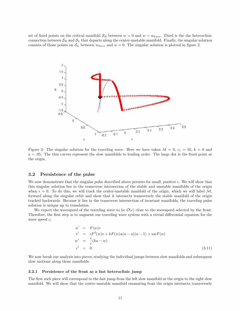
set of fixed points on the critical manifold SR between w = 0 and w = wknee. Third is the the heteroclinicconnection between SR and SL that departs along the center-unstable manifold. Finally, the singular solutionconsists of those points on SL between wknee and w = 0. The singular solution is plotted in figure 2.

Figure 2: The singular solution for the traveling wave. Here we have taken M = 0, c1 = 10, k = 8 anda = .05. The thin curves represent the slow manifolds to leading order. The large dot is the fixed point atthe origin.

3.2 Persistence of the pulse

We now demonstrate that the singular pulse described above persists for small, positive ε. We will show thatthis singular solution lies in the transverse intersection of the stable and unstable manifolds of the originwhen ε = 0. To do this, we will track the center-unstable manifold of the origin, which we will label M,forward along the singular orbit and show that it intersects transversely the stable manifold of the origintracked backwards. Because it lies in the transverse intersection of invariant manifolds, the traveling pulsesolution is unique up to translation.

We expect the wavespeed of the traveling wave to be O(ε) close to the wavespeed selected by the front.Therefore, the first step is to augment our traveling wave system with a trivial differential equation for thewave speed c,

u′ = F (w)v

v′ = cF 2(w)v + kF (w)u(u− a)(u− 1) + uwF (w)

w′ =ε

c(ku− w)

c′ = 0. (3.11)

We now break our analysis into pieces, studying the individual jumps between slow manifolds and subsequentslow motions along those manifolds.

3.2.1 Persistence of the front as a fast heteroclinic jump

The first such piece will correspond to the fast jump from the left slow manifold at the origin to the right slowmanifold. We will show that the center-unstable manifold emanating from the origin intersects transversely

11

the center-stable manifold of the right slow manifold in the plane w = 0. We will use differential forms toshow this intersection is transverse, see [18].

Along the front, the reduced variational equations are given by

δu′ = F (0)δv

δv′ = cF 2(0)δv + F (0)fu(uf , 0)δu+ F 2(0)vδc

δc′ = 0,

where we recall the definition of f(u,w) in (2.1). Here, the δu(η) is a differential one-form acting on η, anelement of the tangent space. Therefore, derivatives apply to the vector η and not to the actual one-form.The relevant stable and unstable manifolds are given by

T(u,v,c)Wcu(0, 0, c∗) = span

〈v, cF (0)v + fu(uf , 0), 0〉, 〈0, h+, 1〉

T(u,v,c)W

cs(1, 0, c∗) = span〈v, cF (0)v + fu(uf , 0), 0〉, 〈0, h−, 1〉

.

We will refer to n as the tangent vector to the solution and we will let η+ = 〈0, h+, 1〉 and η− = 〈0, h−, 1〉for convenience. Since both manifolds share a common solution, they will share the tangent vector n =〈v, cF (0) + fu(uf , 0), 0〉 following this solution. We define the following differential two forms

Puv = δu ∧ δvPvc = δv ∧ δcPuc = δu ∧ δc.

These two forms are bi-linear functionals on the tangent space. Their arguments are vectors that span aplane in R3. When normalized appropriately, these quantities measure the area of the projection of thetracked plane onto the respective coordinate plane (i.e. the u− v coordinate plane for Puv).

At the point of intersection, the two manifolds will intersect transversely if there is no choice of α ∈ Rsuch that,

〈Puv(n, η+), Pvc(n, η+), Puc(n, η

+)〉 = α〈Puv(n, η−), Pvc(n, η−), Puc(n, η

−)〉,

i.e., they are linearly independent. We verify this by computing the differential equations associated to thesedifferential 2-forms. Namely,

P ′uv = cF (0)2Puv + F 2(0)vPuc

P ′vc = cF (0)2Pvc + F (0)fu(uf , 0)Puc

P ′uc = F (0)Pvc.

We can compute explicitly that Puc(n, η+) = Puc(n, η

−) = v. We also note that Puv(n, η±) = vh±. There-

fore, if h+ 6= h−, we will have shown local transversality of these two manifolds. We proceed as follows: first,we use the fact that Puc = v to reduce the first variational equation to

P ′uv = cF 2(0)Puv + F 2(0)v2.

This is solved as

Puv = F 2(0)ecF2(0)ξ

∫ ξ

−∞(e−cF

2(0)τv2(τ))dτ.

Since all terms are positive, we conclude that

Puv(n, η+) = vh+ > 0.

Positivity of v(ξ) implies that h+ > 0. For the manifold W cs, we perform an analogous computation to findthat

Puv = −F 2(0)ecF2(0)ξ

∫ ∞ξ

(e−cF2(0)τv2(τ))dτ,

from which we deduce that h− < 0. Therefore, the two manifolds intersect transversely.

12

3.2.2 Persistence of the segment near the right slow manifold

We will now track M as it passes the right slow manifold. This will require two steps. First, we track Mto a neighborhood of the non-hyperbolic knee using the Exchange Lemma. Then, we use center manifoldtheory and geometric desingularization to track this manifold through a neighborhood of the knee.

Recall the coordinates of the knee,

(u, v, w, c) = (1 + a

2, 0,

k

4(1− a)2, c(0)),

for which we designate wknee = k4 (1 − a)2 and uknee = 1+a

2 . For any δ > 0 define a δ neighborhood of theknee by,

K = (u, v, w, c) | |u− uknee| < δ, |v| < δ, |w − wknee| < δ, |c− c(0)| < δ .

Let br = SR ∩ ∂K. We have the following result.

Lemma 3.1. For fixed δ > 0, the tracked manifold M is C1,O(ε) close to W cu(SR) in a neighborhood ofbr.

Proof: We have that M intersects W cs(SR) transversely on entry into a neighborhood of SR. Theproof is then a standard application of the Exchange Lemma, [19].

We now focus on the dynamics in K. Append to (3.11) a trivial equation for ε. Since c has been fixed toleading order by the front, we ignore the trivial equation for c. Then the point (u, v, w, ε) = (uknee, 0, wknee, 0)is a fixed point for the flow. This fixed point is center-unstable, with one unstable eigenvalue and three zeroeigenvalues. We have the following,

Lemma 3.2. For any k > 0, there exists a local Ck center manifold Cknee of (uknee, 0, wknee, 0), which canbe given as a graph,

v = h(u,w, ε) = b200(u− uknee)2 + b010(w − wknee) +O(ε, (w − wknee)2, (u− uknee)(w − wknee)).

There exists b > 0 and independent of ε, for which the reduced dynamics on Cknee are

uξ = −b(u− uknee)2 − ukneec

(w − wknee) +O(ε, (w − wknee)2, (u− uknee)(w − wknee), (u− uknee)3

)wξ = ε

(kukneec− wknee

c

)+O

(ε, (w − wknee)2, (u− uknee)(w − wknee), (u− uknee)3

)εξ = 0. (3.12)

In addition, to each point p ∈ Cknee there exists an associated, Ck one dimensional unstable fiber Fu(p) givenas a graph over the unstable eigenvector 〈1, cF 2(wknee), 0, 0〉.

Proof. See Appendix A

If δ is sufficiently small, then M and Cknee intersect transversely. Locally, the flow of each point in Mcan be decomposed into the flow of a basepoint in Cknee and a point in the unstable fiber of that basepoint.The flow of the basepoints in the center manifold is equivalent to the normal form for a fold point studiedin [23]. We define the entrance and exit sets,

∆in = (u,w, ε)|w = wknee − ρ2∆out = (u,w, ε)|u = uknee − ρ,

where ρ > 0. We apply verbatim a theorem of [23].

Theorem 2. Let π : ∆in → ∆out be the transition map for the flow of (3.12). Then for all ε ∈ [0, ε0] wehave,

13

1. The manifold Sa,ε passes through ∆out at a point (u,w, ε) = (uknee − ρ, wknee + h(ε), ε) with h(ε) =O(ε2/3).

2. The transition map π is a contraction with contraction rate O(e−C/ε) with C a positive constant.

This leads to the following result.

Lemma 3.3. In a neighborhood of (u, v, w) = (uknee − ρ, h(uknee − ρ, wknee, 0), wknee), M is C1, O(ε2/3)close to the plane w = wknee.

Proof. We establish the C0 result first. Recall thatM is C1 O(ε) close to the smooth manifold W cu(SR) onentry to K. For each ε sufficiently small, this guarantees the existence of a unique pin =M∩ Cknee ∩∆in.Near pin, the dynamics of each point in M can be decomposed into the flow of a basepoint p ∈ Cknee andan expansion in the corresponding unstable fiber Fu(p). Theorem 2 implies that, on exit from K, all of thebasepoints exit K O(e−C/ε) close to πpin or (u,w, ε) = (uknee − ρ, wknee + h(ε), ε). Since the fibers dependsmoothly on their basepoints, the exponential contraction of π implies that each unstable fiber will be locallyO(ε2/3) close to the unstable fiber at (u,w, ε) = (uknee − ρ, wknee, 0). Since the unstable fibers are given asa graph over the unstable eigenvector, whose w component is zero, we have the C0 closeness result.

We now turn to the C1 result. We make the following change of coordinates,

v = v − h(u,w, e), u = u− uknee, w = w − wknee.

In these coordinates, the equation is

uξ = F (w + wknee)(v + h(u,w, ε))

vξ = cF 2(w + wknee)v

wξ = ε

(k(u+ uknee)

c− w + wknee

c

)εξ = 0.

We track the tangent space as it evolves along the trajectory through pin (where v = 0). The variationalequation along this orbit has a simplified form,

δu′ = F (w + wknee) (δv +∇h · 〈δu, δw〉) + F ′(w + wknee)h(u,w, ε)δw

δv′ = cF 2(w + wknee)δv

δw′ =εk

cδu− ε

cδw.

The δv equation has an explicit solution and the subspace δv = 0 is invariant. Restricted to this subspace,we find exactly the variational equation for the center manifold.

δu′ = F ′(w)h(u,w, ε)δw + 2F (w)b200(u− uknee)δu+ b010F (w)δw + η(ε, w, u, δu, δw)

δw′ =εk

cδu− ε

cδw,

where η = O(ε, (w − wknee)δw, (w − wknee)δu, (u − uknee)δw). At pin, the tangent space of M is O(ε)

close to the span of the vectors η1 = 〈1, cF2(wknee−ρ2)

2 + 12

√c2F 4 + 4(fU (U2(wknee − ρ2), wknee − ρ2)), 0〉

and η2 = 〈1, 0,−2ku+ k(1 + a)〉. Let ηc be the restriction of this plane to the tangent space of Cknee at pin.We now consider the differential two forms Puv, Puw and Pvc acting on the vectors η1 and ηc. Then,

Puv(η1, ηc) = δv(η1)δu(ηc)

Pvw(η1, ηc) = δv(η1)δw(ηc)

Puw(η1, ηc) = δu(η1)δw(ηc)− δu(ηc)δw(η1).

Normalize these two-forms by Pσ = PσPuv

. The second statement in Theorem 2 implies that vectors transverse

to the flow are contracted by an exponential amount. Since ηc is close to direction of the flow at pin exits

K exponentially close to the vector pointing in the direction of the flow. This gives δw(ηc)δu(ηc)

= O(ε). Then we

have Puv = 1, Pvw = O(ε) and Puw = O(ε). This establishes the C1 result.

14

3.2.3 Conclusion of the proof of Theorem 1

We have now trackedM to an O(1) distance from the non-hyperbolic knee and shown that it is C1, O(ε2/3)close to the plane w = wknee. Due to the slow w dynamics, this result will still hold as M enters an O(1)neighborhood of SL. We then compareM with the stable manifold of SL. Due to Fenichel Theory, the stablemanifold is tangent to the stable eigenspace of SL. It is easy to verify that this eigenspace has non-zero wcomponent and therefore it must intersect transversely with M. This establishes Theorem 1.

3.3 Further information concerning the decomposition of the wave

We conclude the existence analysis with the following decomposition that will be crucial for the stabilityanalysis. The idea is that at each point the actual solution can always be described as either pointwise (in ξ)close to the singular solution or evolving at an O(ε) rate. To begin, we will decompose R into five intervalscorresponding to different pieces of the solution. Without loss of generality fix ξ = 0 to be the unique pointwhere the wave satisfies u(ξ, ε) = 1/2 and w < 1/2. Now we will define ξr(ε), ξk(ε), ξb(ε), ξl(ε) to be values forwhich the wave transitions from being primarily described by one piece of the singular solution to the next.For example, ξr(ε) describes the value of ξ for which the wave transitions from being described primarilyby the dynamics of the reduced front to where the dynamics are predominately described by the right slowmanifold.

Lemma 3.4. For a particular translate of the homoclinic solution derived in Theorem 1, there exists valuesof the traveling wave coordinate ξ such that the wave profile has the following characterization,

1. On Jf := (−∞, ξr(ε)) and Jb := (ξb(ε), ξl(ε)) the solution satisfies

(u(ξ, ε), w(ξ, e)) = (Uf (ξ) + ε log(ε)U1(ξ, ε),Wf + ε log(ε)W1(ξ, ε)),

(u(ξ, ε), w(ξ, e)) = (Ub(ξ) + ε1/3U1(ξ, ε),Wb + ε1/3W1(ξ, ε))

with U1 = O(1) and W1 = O(1).

2. On Jr := (ξr(ε), ξk(ε)) and Jl := (ξl(ε),∞), we have,

∂

∂ξU(ξ, ε) = O(ε),

∂

∂ξW (ξ, ε) = O(ε).

3. On Jk := (ξk, ξb) we have(u,w) = (Γ,Ω) +O(ε1/3).

Proof: This decomposition is a consequence of the geometric techniques employed in the existenceanalysis, namely Fenichel Theory and geometric desingularization. The tools necessary for the proof can befound in Appendix B.

4 Statement of the Main Stability Result

In this section, we will study the spectral stability of the traveling pulse solution constructed in Theorem 1.We will linearize the system and study the behavior of solutions that are a small perturbation of the travelingpulse. We will establish the following result.

Theorem 3. For each (k, a, c1,M) ∈ Π, there exists ε2 > 0 such that for all 0 < ε < ε2, the travelingpulse solution from Theorem 1 is spectrally stable with a simple zero eigenvalue at λ = 0 due to translationalinvariance of the pulse.

15

Denoting with capital letters the pulse constructed in Theorem 1, we linearize by letting u(ξ, t) = U(ξ) +p(ξ, t) and w(ξ) = W (ξ) + r(ξ, t), substitute these into (3.1) and neglect nonlinear terms,

pt =1

F

∂

∂ξ

(1

Fp′)− cp′ − fU (U,W )p− fW (U,W )r −

(FWF 2

∂

∂ξ

U ′

F

)r − 1

F

∂

∂ξ

(FWU

′

F 2r

)rt = −cr′ + ε(kp− r), (4.1)

where we recall f(u,w) = ku(u − a)(u − 1) + uw. The right hand side of this partial differential equationdefines a linear operator L acting on the vector (p, r)T . We will seek values of λ for which bounded solutionsof the linearized eigenvalue problem L − λI = 0 exist.

The linearized eigenvalue problem is an ordinary differential equation in ξ. It may be written as a systemof first order equations as follows,

p′ = F (W )q

q′ = F (W )(fU (U,W ) + λ)p+ cF 2(W )q + F (W )fW (U,W )r +

(FWF

∂

∂ξ

U ′

F

)r +

∂

∂ξ

(FWU

′

F 2r

)r′ =

kε

cp− λ+ ε

cr. (4.2)

Remark 7. The derivative terms in the right hand side of the equation for q are given by

(FWF

∂

∂ξ

U ′

F)r +

∂

∂ξ(FWU

′

F 2r) =

1

F 2

(2FWU

′′ − 3F 2WU

′W ′

F+ FWWU

′W ′

− (λ+ ε)FWU′

c

)r +

εkFWU′

cF 2p.

We will often denote the right hand side of system (4.2) by A(ξ, λ, ε). In this way, the linearized eigenvalueproblem is equivalent to the system,

dx

dξ= A(ξ, λ, ε)x. (4.3)

Since they satisfy a linear non-autonomous system with well-defined limits as ξ → ±∞, the solutions tothis differential equation can be characterized in terms of exponential dichotomies. Exponential dichotomiesgeneralize the notion of hyperbolicity to non-autonomous systems. The linear system on Cn, is said toposses an exponential dichotomy on an interval J if there exist K,L > 0, α, β > 0 and a linear projectionP (ξ) : R× Cn → Cn satisfying P 2 = P such that the following conditions hold:

X(ξ2, ξ1)P (ξ1) = P (ξ2)X(ξ2, ξ1)

|X(ξ2, ξ1)P (ξ1)| ≤ Ke−α(ξ2−ξ1) for ξ2 ≥ ξ1, ξ1, ξ2 ∈ J|X(ξ2, ξ1)(1− P (ξ1))| ≤ Le−β(ξ1−ξ2) for ξ1 ≥ ξ2, ξ1, ξ2 ∈ J. (4.4)

Here X denotes the fundamental matrix solution of (4.3). The interval J is typically taken to be either R, R+

or R−. We note that on R+, the range of P is chosen uniquely as the space of all initial data that convergesexponentially to zero as ξ →∞. The nullspace of this projection operator is not unique however. Likewise,on R− it is the nullspace of the projection operator (1−P ) that is uniquely determined as the space of initialdata converging exponentially to zero in backwards time. Only on R are the range and nullspace of P bothchosen uniquely. The Morse index of an exponential dichotomy measures the dimension of the null space ofthe stable projection. When the exponential dichotomy is posed on a half line, we refer to i+ and i− as theMorse indices of the exponential dichotomies on either half line. Since we are only concerned with the caseof traveling pulses which are homoclinic orbits in (4.3), we have that i+ = i−. Exponential dichotomies canbe used to whenever there exists a gap between the exponential rates on two different subspaces. In thisway, it is not necessary that α and β always be positive, but only that −α < β. Exponential dichotomiesand properties ensuring their existence have been studied in great detail. We have collected some relevantTheorems in Appendix C.

Spectral properties of L, namely invertibility of L − λ in a Banach Space, can be restated in terms ofproperties of exponential dichotomies of (4.3). In particular, the spectrum of σ(L) can be characterized by(see [28, 29]):

16

• λ is in the resolvent set if and only if (4.3) has an exponential dichotomy on R.

• λ is in the essential spectrum if A∞ := limξ→±∞A(ξ, λ) is not hyperbolic, or if A∞ is hyperbolic butthe Morse indices are not equal, i.e. i+ 6= i−.

• λ is in the point spectrum if (4.3) has exponential dichotomies on both R+ and R− but not on R. Inother words, letting P+ be the stable projection for R+ and letting P− be the stable projection forR− we have that

rng(P+) ∩ ker(P−) 6= ∅.

Given this characterization, the essential spectrum can be located using only information about the asymp-totic system A∞. The point spectrum is more elusive. We will make use of the Evans Function,

D(λ) = rngP+(0) ∧ rng(1− P−(0)), (4.5)

see Chapter 4 in [34]. The Evans function is an analytic function defined on the complement of the essentialspectrum having zeros for values of λ in the point spectrum. In addition, the order of λ as a zero of D(λ)corresponds to the algebraic multiplicity of the eigenvalue. The analyticity of D(λ) is the key feature, asarbitrarily small analytic perturbations of D(λ) will retain the same number of zeros.

5 Preliminary Spectral Analysis

5.1 The essential spectrum

We begin our analysis of the spectrum by computing the essential spectrum. Recall that the essentialspectrum is characterized by the values of λ for which the asymptotic matrix A∞ has eigenvalues on theimaginary axis. Here,

A∞(λ) =

0 1 + M2c1

0

(ka+ λ)(1 + M2c1

) c(1 + M2c1

)2 0εkc 0 −λ+ε

c

.

Thus,

σess = icl − ε : l ∈ R ∪ − l2

(1 + M2c1

)2− icl − ka : l ∈ R. (5.1)

The essential spectrum is plotted in Figure 3. The quadratic part, which has a vertex at λ = −ka, is alwaysbounded strictly in the left half plane. The vertical component will converge to the imaginary axis as ε→ 0.We also note that for λ = 0, the fixed point at (p, q, r) = (0, 0, 0) has one positive eigenvalue and two negativeeigenvalues for all λ with Re (λ) > −ε.

5.2 The reduced spectra along the front and back

The spectra of the reduced problems along the front and the back will be of critical importance as weconstruct the Evans Function for the full system. We will discuss the case of the front first. Recall that thereduced problem along the front is given by setting ε = 0 in (3.1). In this case, we have that w is a constant,which along the front is given by w = 0. The equation for u is

∂2u

∂ξ2− cF 2(0)

∂u

∂ξ− F 2(0)ku(u− a)(u− 1) = 0.

The reduced linear eigenvalue problem along the front is given by

Lfp :=∂2p

∂ξ2− cF 2(0)

∂p

∂ξ− F 2(0)fU (Uf (ξ), 0)p = λp.

The spectrum of this Sturm-Liouville operator has been studied in [12], where it was shown that the spectrumof Lf has an isolated eigenvalue with algebraic multiplicity one at λ = 0. Therefore, we may define a reduced

17

Figure 3: An illustration of (5.1), the boundary of the essential spectrum in the complex plane. Theparameters used here are ε = .01, k = 8, a = .05, c1 = 10 and M = 1.

Evans function for the front, DF (λ). This function is analytic on a region that includes all of the right halfof the complex plane as well as a vertical strip of the left half-plane. DF (λ) has a simple zero at λ = 0. Allother zeros lie in the left-half plane.

Analogously, the reduced equation along the back is given by,

∂2u

∂ξ2− cF 2(Wb)

∂u

∂ξ− F 2(Wb)ku(u− U2(Wb))

2 = 0.

The linearized eigenvalue problem for the reduced problem along the back is given by

Lbp :=∂2p

∂ξ2− cF 2(Wb)

∂p

∂ξ− F 2(Wb)fU (Ub(ξ),Wb)p = λp.

The spectrum of this operator was studied in [37]. The boundary of the essential spectrum is again givenby the values of λ for which the limiting system has purely imaginary eigenvalues. Since fU = 0 at theknee, we get that the set −l2 + icF 2(Wb)l : l ∈ R is one such curve (the other curve lies strictly in thestable half-plane). As a result, we have that λ = 0 is an element of the essential spectrum of Lb. Thederivative of the wave ∂ξUb(ξ) solves the linearized eigenvalue problem at λ = 0. This solution connects thecenter-unstable subspace at ξ = −∞ to the stable subspace at ξ = ∞. Thus, one finds that the unstablesubspace is preserved. The authors in [37] defined an Evans function DB(λ) for the reduced problem alongthe back. This analytic Evans function is non-zero to the right of the essential spectrum of the back. Usingexponential weights, one finds that there exists an analytic extension of DB(λ) into the essential spectrum.This analytic extension was found to be non-zero for all values of λ in a suitable neighborhood of the origin.At first glance one may expect an embedded eigenvalue at λ = 0 due to the derivative of the reduced waveprofile satisfying the eigenvalue equation. This is not the case however as the Evans function measuresconnections between the unstable subspace at ξ = −∞ and the stable subspace at ξ = ∞. The derivativeof the wave U ′b connects the center-unstable subspace at ξ = −∞ to the stable subspace at ξ = ∞. In thisway, the unstable connection is seen to exist for all λ in a neighborhood of the origin.

5.3 The regime of large |λ|In this section, we show the non-existence of point spectrum for the eigenvalue problem when Re λ > −εand |λ| large. This will allow us to restrict to a compact subset of the complex plane in the analysis of

18

section 6. For values of λ in this compact set, we will be able to select the constants for our exponentialdichotomies in a consistent, O(1) manner. The fact that λ which are large in modulus do not contribute tothe spectrum is well established. Evans proved a result along these lines in his original work [10]. We willfollow a similar argument of Sandstede, see Section 4.2.2 of [34]. The key idea is that as λ becomes large inmodulus, it dominates the stability problem and it is no longer possible to have a solution that is boundedin both asymptotic limits.

To see this, we rescale the linearized eigenvalue problem (4.2) as

τ =√|λ|ξ, P = p, Q =

q√|λ|, R = r.

This transforms (4.2) into

P = F (W )Q

Q =λ

|λ|F (W )P +O(

1√|λ|

)

R =−λc√|λ|R+O(

ε√|λ|

). (5.2)

Neglecting the higher order terms, the linearized eigenvalue problem at τ = ±∞ is hyperbolic with eigenvalues

±√

λ|λ|F (0) and − λ

c√|λ|

. Since the only τ dependence in (5.2) to leading order in√|λ|−1

is through the

slowly varying W (τ), the leading order equation varies slowly in τ and Theorem 9 in Appendix C can beapplied to find the existence of an exponential dichotomy on all of R. Then, Theorem 7 implies that thisdichotomy persists for the full system. Recalling our previous discussion, this implies that the Evans functionD(λ) is non-zero for large λ with Re (λ) > 0. For λ on the imaginary axis, the eigenvalue − λ

c√|λ|

becomes

imaginary as the essential spectrum is approached. However, it is easy to see that if one is willing to relax thehyperbolicity condition in Theorem 9 the same results apply provided that an spectral gap persists betweenthe stable and unstable eigenvalues. In fact, this argument can be used to analytically extend the Evansfunction a small distance into the left half plane.

To summarize, we have shown that for all 0 < ε < ε0, there exists constants K > 0 and b > 0 such thatthe Evans function has an analytic continuation with D(λ) 6= 0 for all |λ| ≥ K with Re (λ) > −b.

5.4 Restriction to a compact set

From this point forward, we are interested in the existence of point spectra in the set

Ω := λ ∈ C|Re (λ) > −δ, |λ| < K.

We will remark on the constant δ in a moment. Our proof will ultimately rely on Rouche’s Theorem tocount the number of zeros of the analytic Evans function D(λ) in a neighborhood of the origin. Since theessential spectrum accumulates on the imaginary axis, this necessitates the analytic extension of D(λ) intothe essential spectrum. As we noted above, such an extension is possible provided a spectral gap betweenthe eigenvalues of A∞(λ) persists. In fact, it is convenient for the analysis if this spectral gap exists forall values of ξ ∈ R. We denote the three eigenvalues of A(ξ, λ, ε), which may also be referred to as spatialeigenvalues, by,

µu(ξ, λ) =cF 2(W )

2+

1

2

√c2F 4 + 4(fU (U,W ) + λ)

µs(ξ, λ) =cF 2(W )

2− 1

2

√c2F 4 + 4(fU (U,W ) + λ)

µc(λ) =−λc. (5.3)

The constant δ(k, a, c1,M) will be selected so that the following properties hold:

19

1. DF (λ) 6= 0 for all λ|Re λ > −δ except at λ = 0

2. DB(λ) 6= 0 for all λ|Re λ > −δ (see [37])

3. For all ξ ∈ R, there is a spectral gap between the stable (µs(ξ, λ), µc(ξ, λ)) and unstable (µu(ξ, λ))eigenvalues, see (5.3). In particular, we will require

0 < δ < min

ka,

k(1 + a)2

24

.

We recall that DF (λ) and DB(λ) are defined in Section 5.2. Verifying that the final condition on δ impliesthe existence of a spectral gap will be delayed until the proof of Theorem 3 (see (6.3) and (6.6)).

6 Proof of Theorem 3

In this section, we construct exponential dichotomies that describe the evolution of the linearized eigenvalueproblem (4.2) over each of the intervals Jf , Jr, Jk, Jb, Jl defined in section 3.3. These exponential dichotomieswill be the fundamental objects used to track the stable and unstable subspaces needed for the Evans function.The proof will draw heavily on well known roughness of dichotomy results, which we have collected inAppendix C.

6.1 Exponential dichotomy for the front

Recall that we have fixed ξ = 0 to be the unique value of ξ for which the wave satisfies u = 1/2 and w < 1/2.For values of ξ ∈ Jf = (−∞,−θf log(ε)), Lemma 3.4 implies

U(ξ) = Uf (ξ) + ε log(ε)U1(ξ, ε)

W (ξ) = Wf + ε log(ε)W1(ξ, ε),

where |U1|, |W1| < Mf , with Mf (k, a, c1,M) chosen independently of ε. Again, let x = (p, q, r)T and writethe linearized eigenvalue equation (4.3) as the system,

x′ = (A(ξ, λ, 0) +B(ξ, λ, ε))x. (6.1)

where B(ξ, λ, ε) = A(ξ, λ, ε)−A(ξ, λ, 0) for ξ ∈ Jf . In particular,

A(ξ, λ, 0) =

0 F 0F (fU (Uf ,Wf ) + λ) cF 2 FfW (Uf ,Wf ) + 2FWF 2 U

′′f − λ

cF 2FWU′f

0 0 −λc

B(ξ, λ, ε) =

0 F1 0b21 2cFF1 b23εkc 0 − εc

b21 = F1(fU + λ) + FfUUU1 + FfUWW1 +

εkFWU′′

cF 2

b23 = F1fW −3FWU

′W ′

F 3+FWWU

′W ′

F 2− FWU

′

cF 2.

Here terms of the form F1 refer to the first variation of F , i.e. F1 = F (W (ξ))−F (Wf ). Note that all termsin B(ξ, λ, ε) are at most O(ε log(ε)).

We will first construct an exponential dichotomy on R± for the singular system

z′ = A(ξ, λ, 0)z, (6.2)

for all values of λ ∈ Ω with constants K0(λ), L0(λ), α0(λ) and β0(λ). We will then show that theseexponential dichotomies persist for the flow of the full system with constants K(λ), L(λ), α(λ) and β(λ),

20

albeit only on the asymptotically large interval Jf . A key point will be to show that these constants can bedefined to be O(1) in ε. Finally, we will show that these constants may also be chosen independent of λ ∈ Ω.This will imply the existence of an exponential dichotomy on Jf with projection Qf (ξ, λ, ε) and constants,

Kf = supλ∈Ω

K(λ), Lf = supλ∈Ω

L(λ), αf = infλ∈Ω

β(λ), βf = infλ∈Ω

β(λ).

To begin, the singular system has asymptotic limits,

A± = limξ→±∞

A(ξ, λ, 0) =

0 F 0F (fU (U±,Wf ) + λ) cF 2 FU±

0 0 −λc

.

The eigenvalues, µ(λ)±, of the asymptotic matrices A± satisfy the condition,(−λc− µ±

)((µ±)2 − cF 2µ± − F 2(fU (U±,Wf ) + λ)

)= 0.

We label the three roots µ±u , µ±s and µ±c and their corresponding eigenvectors v±u , v±s and v±c . Note thatµ±c = −λc , as in (5.3). For Re(λ) > 0, µ±u is the sole unstable eigenvalue for A±. For −δ < Re (λ) < 0, µ±cis also unstable. There is no problem, so long as a spectral gap exists between µ±c and µ±u . Both asymptoticlimits for the singular problem correspond to points on a stable branch of the slow manifold wherein wehave fU > 0. In particular, fU (U±,Wf ) > ka for the front. Therefore, µ±u (λ) > cF 2(0) > µ±s (λ), wheneverδ < ka. We must simply verify that δ

c < cF 2(0). This follows since,

δ <k

24(1 + a)2 <

16k

24

(F (Wb)

F (0)

)2(1

2− a)2

< (cF (Wb))2 < (cF (0))2, (6.3)

where the first inequality follows from our assumptions on Ω and the second follows from the assumptionthat the critical wavespeed for the back is less than the wavespeed selected by the front. In this way, theasymptotic eigenvalues have a spectral gap between the unstable and weakly-unstable eigenvalues for allξ ∈ Jf when −δ < Re (λ) < 0.

Note that A(ξ, λ, 0) has an invariant subspace given by r = 0. Let y = (p, q)T and consider the reducedsystem restricted to this subspace,

y′ = AR(ξ, λ)y.

Values of λ for which there exist bounded solutions on R to this equation correspond to spectral values ofthe linearized operator Lf along the front, recall the definition in Section 5.2. We have that σ(Lf ) ∩Ω atthe single point λ = 0. This implies that the reduced system has an exponential dichotomy on both halflines, R+ and R−, for all λ ∈ Ω. Let P±R (ξ, λ) : R × C2 → C2 be the projection operator for the reducedsystem associated to the exponential dichotomies. For all λ 6= 0, we may choose P+

R (0, λ) = P−R (0, λ). Wewill show that (6.2) also has this property.

Lemma 6.1. For each λ ∈ Ω, the linear system (6.2) has an exponential dichotomy on R± with con-stants K0(λ), L0(λ), stable decay rate α0 < minλ∈ΩRe λ

c ,−Re µ±s (λ), unstable decay rate β0(λ) =

infλ∈ΩRe µ±u (λ), and analytic projections P±f (ξ, λ) satisfying P+f (ξ, λ) = P−f (ξ, λ) for all λ 6= 0. Fi-

nally, we have |P+f (ξr, λ)− P+

∞(λ)| = O(ε) where P+∞(λ) is the stable spectral projection for the asymptotic

system A+.

Proof: We consider the case of R+, the situation for R− is similar. Choose α0 so that

maxλ∈ΩRe (µc(λ)),Re (µ±s (λ)) < −α0 < min

λ∈ΩRe (µ±u (λ)).

By the estimates in (6.3) such a choice is possible. Let P+∞(λ) be the spectral projection associated to the

eigenvalues µ+c and µ+

s . It is clear that x′ = A+(λ)x has an exponential dichotomy on R+ for any valueof λ ∈ Ω (allowing α < 0 if necessary). We note that the constants K0(λ) and L0(λ) are continuous withrespect to λ. This is observed since

etA+(λ)P∞+ =

1

2πi

∫γ

(A+(λ)− zI)−1etzdz,

21

where γ is a closed curve in C surrounding µ+c (λ) and µ+

s (λ) for all λ ∈ Ω, with maximal real part −α0 sothat it does not enclose any µ+

u (λ). Then

|etA+(λ)P∞+ | ≤

1

2π

∫γ

|(A+(λ)− zI)−1||dz|e−α0t,

so that

K0(λ) =1

2π

∫γ

|(A+(λ)− zI)−1||dz|,

and is continuous in λ. Let C(ξ, λ) = A(ξ, λ, 0) − A+(λ). Then |C(ξ, λ)| ≤ Cfe−dξ as ξ → ∞ for some

d > 0 and Theorem 8 implies that (6.2) has an exponential dichotomy on R± with the same decay rates asthe limiting system, A+. This establishes the first part of the lemma, for the remainder we appeal to themechanics of the proof of Theorem 8.

Without loss of generality, assume that the stable and unstable decay rates are equal and are α(λ). Selectξ0 so large that

∫∞ξ0|C(τ, λ)|dτ < 1/(2K0(λ)). Then the following operator T is a contraction map on the

space of continuous, bounded matrix functions of R+,

Tφ(ξ, ξ0) = eA+∞(ξ−ξ0)P+

∞ +

∫ ξ

ξ0

eA+∞(ξ−τ)P+

∞C(τ, λ)φ(τ, ξ0)dτ −∫ ∞ξ

eA+∞(ξ−τ)(1− P+

∞)C(τ, λ)φ(τ, ξ0)dτ.

The unique fixed point, φ∗ defines the stable projection at ξ0, i.e. P+f (ξ0) = φ∗(ξ0, ξ0). The projection at

other values of ξ can be found using the flow property, see (4.4). This leads to the following equality,

P+f (ξ, λ)− P+

∞(λ) = −∫ ξ

ξ0

eA+∞(ξ−τ)P∞+ (λ)C(τ, λ)X(τ, ξ)(1− P+

f (ξ, λ))dτ

−∫ ∞ξ

eA+∞(ξ−τ)(1− P∞+ )C(τ, λ)X(τ, ξ)P f+(ξ, λ)dτ.

Here X(ξ, ξ0) is the fundamental matrix solution for (6.2). Since ξr = −θf log(ε), for θf arbitrary but O(1),we may select θf so that |P+

f (ξr, λ) − P∞+ | = O(ε) holds. Note that the spectral projection P+∞ depends

analytically on λ. The projection P±f (ξ, λ) is also analytic since it is given as the limit of analytic functionsthat converge uniformly on Ω.

The range of Pf (ξ, λ) is unique, but its nullspace is not. By the above construction, we have kerPf (ξ0, λ) =kerP+

∞(λ). The same analysis applies if we were to start with a different projection Pnew∞ (ξ, λ) for the asymp-totic system, A+. In particular, we still have |P+

f (ξr, λ) − P+∞(λ)| = O(ε) since |P+

f (ξr, λ) − Pnew∞ (ξr, λ)|behaves as before and |Pnew∞ (ξ, λ)− P+

∞(λ)| goes to zero exponentially as ξ →∞.We now consider all of R. The subspace r = 0 is invariant and an exponential dichotomy exists there

on R±. It only remains to show that the final direction can be chosen appropriately. This follows since thestable projection on the positive half-line is unique and must have component in the r direction. Thus, thereis a stable projection on R± and it is given by

P±f (ξ, λ) =

(P±R (ξ, λ) v(ξ, λ)

0 1

). (6.4)

The matrix is written in block form, so v is a two dimensional vector. Finally, for all λ ∈ Ω, λ 6= 0, wemay select P+

f (λ) = P−f (λ) and an exponential dichotomy then exists on all of R with the appropriatemodifications of the unstable and stable decay rates.

We now analyze the full problem (6.1) over the front for sufficiently small ε. Divide the interval Jf intotwo pieces:

J−f := (−∞, 0), J+f := (0,−θf log(ε)).

22

Lemma 6.2. For all (k, a, c1,M) ∈ Π, there exists an εf > 0 such that for all 0 < ε < εf and λ ∈ Ω, theequation (6.1) has an exponential dichotomy on R± with analytic stable projections Q±f (ξ, λ, ε) and constants

K(λ), L(λ), α(λ) and β(λ). Furthermore, K and L are O(1) with respect to ε, β(λ) = β0(λ) +O(ε log(ε))α(λ) = α0(λ) +O(ε log(ε)) and Q±f (ξ, λ, ε) = P±f (ξ, λ) +O(ε log(ε)).

Proof: The existence of the exponential dichotomy follows from standard roughness of dichotomyresults, see Theorem 7. The one subtlety is the fact that for ε small but non-zero, the interval J+

f is finite,so exponential dichotomies exist there trivially for any choice of the projection. To avoid this problem, weexpand J+

f to all of R+ in such a way that |B(ξ, λ, ε)| = O(ε log(ε)) for all ξ ∈ R+. Following the proof ofProposition 4.1 in [6], the unique bounded matrix solution to the full problem is given as the fixed point ofthe following integral equation,

Tφ(ξ) = X(ξ, ξ0)P+f (ξ0, λ) +

∫ ξ

ξ0

X(ξ, s)P+f (s, λ)B(s)φ(s)ds

−∫ ∞ξ

X(ξ, s)(1− P+f (s, λ))B(s)φ(s)ds.

It is easy to show that this constitutes a contraction mapping on the space of uniformly continuous, boundedmatrix functions on R+ with contraction constant θ = O(ε log(ε)). The unique fixed point of the mapping isgiven by φ∗(s). The stable projection for the perturbed system is then given by Q+

f (ξ0, λ, ε) = φ∗(ξ0) and the

estimate Q±f (ξ, λ, ε) = P±f (ξ, λ) +O(ε log(ε)) follows from [6]. When restricted to Jf , the projection is not

unique. However, any two different projections differ by only O(ε1+θfβ0

log(ε)) amounts. If the extension toall of R+ was done so that B(ξ, λ, ε) is analytic in λ for all ξ ∈ R+ then the projection Q+

f (ξ, λ, ε) is analyticas well. In addition, we have (see Proposition 4.1 in [6])

L(λ) =2(L0)2

1 + 2L0 + (1 + 2L0)√

1− 2θ − 4L0, K(λ) =

2(K0)2

1 + 2K0 + (1 + 2K0)√

1− 2θ − 4K0

β(λ) = β0√

1− 2θ , α(λ) = α0√

1− 2θ,

where we see that K(λ) and L(λ) are both O(1) and β(λ) = β0 +O(ε log(ε)) and α(λ) = α0 +O(ε log(ε)).

This establishes uniformity of the exponential dichotomies with respect to ε. To show the same for λ, wewill need to define new constants

Kf = Lf = supλ∈Ω

L(λ), βf = infλ∈Ω

β(λ), αf = infλ∈Ω

α(λ).

The αf and βf are O(ε log(ε)) close to α0(λ) and β0(λ). In turn, these attain their minimum on the boundaryof Ω, at λ = −δ. Since there is a spectral gap at this point, there remains a spectral gap between αf andβf for sufficiently small values of ε.

To recap, we have shown that there exists Q±f (ξ, ε, λ), Kf , Lf , αf and βf so that

|X(ξ2, ξ1)Q±f (ξ1, ε, λ)| ≤ Kfe−αf (ξ2−ξ1) for ξ2 ≥ ξ1 ξ1, ξ2 ∈ J±f

|X(ξ2, ξ1)(1−Q±f (ξ1, ε, λ))| ≤ Lfe−βf (ξ1−ξ2) for ξ1 ≥ ξ2 ξ1, ξ2 ∈ J±f .

This has been shown along the front. We conclude the analysis of the front with an important observation.

Corollary 1. The subspace of solutions for the full system that converge to the origin as ξ → −∞ is givenexactly by the range of Q−f . In other words,

P−(0, λ, ε) = Q−f (0, λ, ε).

23

6.2 The Back

To construct an exponential dichotomy for the solution of the eigenvalue problem along the back we would liketo follow the same approach as that of the front. In that situation, the exponential decay of the leading ordersolution to the rest points along the slow manifold allowed for the construction of a leading order exponentialdichotomy with decay rates specified by the exponential behavior of the rest state. A perturbation argumentwas then used to extend this dichotomy to the full system, albeit on a smaller, asymptotically large domainin ξ. We will use the same general approach for the back, however, the algebraic instead of exponentialdecay of the solution to the knee will complicate the analysis considerably.

We begin the analysis of the back by introducing a new variable, χ. We will select χ = 0 to correspond to

the unique point along the back where U = (1+a)3 . In this way, the interval Jb = (ξb(ε), ξl(ε)) in ξ corresponds

to an interval in χ of the form (− θkε1/3

,−θl log(ε)). In terms of this new variable, we have that

U(χ) = Ub(χ) + ε1/3U1(χ, ε)

W (χ) = Wb + ε1/3W1(χ, ε),

with |U1| and |W1| bounded by a constant Mb, independent of ε. As we did for the front, our approach willconsist of three steps. First, we consider the reduced (w = Wb), singular (ε = 0) case and show that thissystem has an exponential dichotomy for all λ ∈ Ω. Second, we extend this exponential dichotomy in thesingular case to all three dimensions. Finally, we show that this solution persists using Theorem 7.

Following subsection 6.1 we write the linearized eigenvalue problem as

x′ = (A(χ, λ, 0) +B(χ, λ, ε))x, (6.5)

for x = (p, q, r)T . The singular system is given by

A(χ, λ, 0) =

0 F 0F (fU (Ub,Wb) + λ) cF 2 FfW (Ub,Wb) + 2FWF 2 U

′′b − λ

cF 2FWU′b

0 0 −λc

.

Let A± = limχ→±∞A(χ, λ, 0). As was the case with the front, the r = 0 subspace is invariant under thesingular flow. The dynamics in this invariant subspace is given by the system y′ = AR(χ, λ)y with

AR(χ, λ) =

(0 F (Wb)

F (Wb)(fU (Ub,Wb) + λ) cF (Wb)2

).

This system is precisely the linearized eigenvalue problem associated to the Fisher-type equation for thejump back. The spectrum of this systems has been studied in [37], the results of which are summarized inthe following lemma.

Lemma 6.3. Fix (k, a,M, c1) ∈ Π. For all λ ∈ Ω, the system y′ = AR(χ, λ)y has an exponential dichotomyon R with projection P bR(χ, λ).

Proof: The proof follows the one contained in [37], where n-degree Fisher equations were studied. Itcan be summarized as follows. The existence of a spectral gap between the limiting eigenvalues is shown.The slow algebraic decay prevents the direct application of Theorem 8, since A(χ, λ, 0)−A− is not integrable.The existence of a spectral gap for all χ < 0 allows for a diagonalization of the leading order system. Thissystem can be solved by exponentiation and the decay rates can be bounded in this way. The next ordercorrection now involves derivatives of the linearizing transformation and therefore it converges with at leastrate O(C/χ2) and Theorem 8 can now be applied. This establishes an exponential dichotomy and thenSturm-Liouville arguments can be applied to show that this exponential dichotomy may always be extendedto all of R (i.e there exists DB(λ) 6= 0).

We must show that the same technique may be applied consistently for all parameter values in Π, that is,we must demonstrate the existence of a spectral gap between the frozen eigenvalues so that the diagonalizationstep is justified. The remainder of the proof follows as in [37]. Recall that at the knee (U,W ) = (uknee, wknee),we have fU (uknee, wknee) = 0. In addition, we have that fU (Ub,Wb) < 0 close to the knee. Near the left most

24

side of Ω we must ensure that a spectral gap exists between µu and µs (a gap between µu and µc was shownin (6.3)). In other words, we must show that the Re (c2F (Wb)

4 + 4F (Wb)2(fU (Ub,Wb) + λ)) > 0. Any easy

calculation finds that fU (Ub,Wb) attains its minima at Umin = 13 (1+a) and that fU (Umin,Wb) = −k

12 (1+a).Then,

c2F (Wb)4 + 4F (Wb)

2fU (Umin,Wb) = F (Wb)2

(2k(1 + a)2F (Wb)

2

F (0)2− k(1 + a)2

3

)= k(1 + a)2F (Wb)

2

(2F (Wb)

2

F (0)2− 1

3

)≥ k(1 + a)2F (Wb)

2

6(6.6)

The last inequality follows since 2F (Wb) > F (0) for parameters in Π. Then, selecting 0 < δ < k(1+a)2

24implies that Re (µu(ξ, λ)) > Re (µs(ξ, λ)) for ξ along the back and λ ∈ Ω. Due to this spectral gap, thereexists a diagonalizing transformation Q(χ, λ), and the proof in [37] can be extended.

We do not remark on the analyticity of the projection P bR, although it is also studied in [37]. This isbecause we will only use the projection along the back as a skeleton by which to track the analytic projectionP+(0, λ, ε) and this process will not require analyticity of P bR. Next, we extend these exponential dichotomiesto all of C3.

Lemma 6.4. Fix (k, a,M, c1) ∈ Π. For all λ ∈ Ω, the singular problem z′ = A(χ, λ, 0)z has an exponentialdichotomy on R with projections Pb(χ, λ) and constants K0

b (λ), L0b(λ), α0

b(λ) and β0b (λ). In addition, we have

|Pb(ξb, λ) − Pknee(λ)| = O(ε1/3) and |Pb(ξl, λ) − P+b,∞(λ)| = O(ε) where Pknee(λ) is the spectral projection

associated to stable eigenvalues of A− and P+b,∞(λ) is the same for A+.

Proof: We proceed as we did for the front. The exponential convergence of A(χ, λ, 0) to its asymptoticstate as χ → ∞ implies that the analysis will be identical to that of the front for R+. Thus, we considerχ < 0. Due to the slow convergence of A(χ, λ, 0) to its asymptotic state as χ→ −∞, it is again not possibleto apply Theorem 8 and find an exponential dichotomy with the same decay rates as A−. However, we recallthat the spectral gap between unstable and weakly unstable eigenvalues persists for the full system due tothe calculation in (6.3). This gives the existence of α0

b and β0b such that

maxλ∈ΩRe (µc(λ)),Re (µs(χ, λ)) < −α0

b < β0b < min

λ∈ΩRe (µu(χ, λ)).

Let C(χ, λ) = A(χ, λ, 0)− A−. To show the existence of an exponential dichotomy, we set up a fixed pointequation as we did before,

Tφ(χ, χ0) = eA−(χ−χ0)(1− Pknee)−

∫ χ0

χ

eA−(χ−τ)(1− Pknee)C(τ, λ)φ(τ, χ0)dτ

+

∫ χ

−∞eA−(χ−τ)PkneeC(τ, λ)φ(τ, χ0)dτ.

We can not apply Theorem 8 (C(χ) is not integrable). Instead we fix χ0 < 0 large enough so that we mayapply Theorem 7 to conclude the existence of an exponential dichotomy with decay rates α0

b and β0b (see also

[31] for a similar argument using Fredholm properties). The unique fixed point of the operator, Tφ, when

25

evaluated at χ = χ0 is the unstable projection (1− Pb(χ0, λ)). Now we have,

(1− Pb(χ, λ)) = X(χ, χ0)(1− Pb(χ0, λ))X(χ0, χ) = φ∗(χ, χ0)X(χ0, χ)

= eA−(χ−χ0)(1− Pknee)X(χ0, χ)−

∫ χ0

χ

eA−(χ−τ)(1− Pknee)C(τ, λ)φ∗(τ, χ0)X(χ0, χ)dτ

+

∫ χ

−∞eA−(χ−τ)PkneeC(τ, λ)φ∗(τ, χ0)X(χ0, χ)dτ

= (1− Pknee) +

∫ χ0

χ

eA−(χ−τ)(1− Pknee)C(τ, λ)X(τ, χ)dτ

−∫ χ0

χ

eA−(χ−τ)(1− Pknee)C(τ, λ)φ∗(τ, χ0)X(χ0, χ)dτ

+

∫ χ

−∞eA−(χ−τ)PkneeC(τ, λ)φ∗(τ, χ0)X(χ0, χ)dτ

= (1− Pknee) +

∫ χ0

χ

eA−(χ−τ)(1− Pknee)C(τ, λ)X(τ, χ)Pb(χ, λ)dτ

+

∫ χ

−∞eA−(χ−τ)PkneeC(τ, λ)X(τ, χ)(1− Pb(χ, λ))dτ.

The algebraic decay of the solution to its asymptotic limit implies that there exists a Kc > 0 so that for allτ < χ0 we have |C(τ, λ)| ≤ −Kcτ . Then,

|Pb(χ, λ)− Pknee(λ)| ≤ K0KKc

∫ χ0

χ

e−(β0b+α0

b)(τ−χ)

−τdτ + L0LKc

∫ χ

−∞

e−(α0b+β

0b )(χ−τ)

−τdτ

≤ K

(β0b + α0

b)|χ|+ Ke(β0

b+α0b)χ

∫ χ0

χ

e−(β0b+α0

b)τ

(β0b + α0

b)τ2dτ +

L

(α0b + β0

b )|χ|,

where we have integrated by parts and neglected negative terms in the first integral. Since χ0 is fixed, wehave for χ < 0 and sufficiently large, the second integral is dominated by its value at χ. This leads to thefollowing characterization,

|Pb(χ, λ)− Pknee(λ)| = O(|χ|−1) as χ→ −∞.

Since, χk = −θkε−1/3, this implies that |Pb(χk, λ)− Pknee(λ)| = O(ε1/3) as required. As was the case withthe front, changing the range of (1− Pb(χ, λ)) (the nullspace of Pb(χ, λ)) does not affect the results.

This leads to the following result.

Lemma 6.5. For all λ ∈ Ω and ε sufficiently small, the system (6.5) has an exponential dichotomy on Jbwith projection Qb(ξ, λ, ε) and constants Kb, Lb, αb, and βb. Furthermore, we have that

|Qb(ξb, λ, ε)−Qk(ξb, λ, ε)| = O(ε1/3).

Proof: The persistence of the dichotomy for small ε 6= 0 is a consequence of the roughness of expo-nential dichotomies as in the case of the front, see Theorem 7.

6.3 The Right Slow Manifold

In this section, we will show the existence of an exponential dichotomy for the solution of the linearizedeigenvalue for all ξ ∈ Jr and ε sufficiently small. We have the following result,

26

Lemma 6.6. For all (k, a, c1,M) ∈ Π there exists an εr such that for all 0 < ε < εr the linearized eigenvalueproblem x′ = A(ξ, λ, ε)x has an exponential dichotomy on Jr with projection Qr(ξ, λ, ε) and constants, Kr,Lr, αr < infξ∈Jr,λ∈Ω minRe (−µs(ξ, λ)),Re −λc and βr < infξ∈Jr,λ∈Ω Re µu(ξ, λ), all defined O(1) withrespect to ε. If Pr(ξ, λ) is the spectral projection for A(ξ, λ, ε) for each ξ ∈ Jr, then we have |Qr(ξ, λ, ε) −Pr(ξ, λ)| = O(ε) for all ξ ∈ Jr.

Proof: Along the slow manifold, the linearized eigenvalue problem varies slowly with ξ. The existenceof an exponential dichotomy with the above properties is a direct result of Theorem 9, see Proposition 6.1in [6].

We conclude with a result that compares the projections at the transition point between the front andthe right slow manifold.

Lemma 6.7. For all λ ∈ Ω and ε sufficiently small, we have,

|Qf (ξr, λ, ε)−Qr(ξr, λ, ε)| = O(ε log(ε)). (6.7)

Proof: From Lemma 6.1, Lemma 6.2 and Lemma 6.6,

|P+f (ξr, λ)− P+

∞(λ)| = O(ε)

|Qf (ξr, λ, ε))− P+f (ξr, λ)| = O(ε log(ε))

|Qr(ξr, λ, ε)− Pr(ξr, λ)| = O(ε).

Note that Pr(ξr, λ) = P+∞(λ) since both are the spectral projection of the linearized eigenvalue problem at

ε = 0 and (U,W ) = (1, 0). The result follows.

6.4 The Left Slow Manifold

The analysis along the left slow manifold is similar to that of the right slow manifold. Therefore, we have

Lemma 6.8. For all λ ∈ Ω and ε sufficiently small, the linearized eigenvalue problem on (ξl(ε),∞) has anexponential dichotomy with analytic projection Ql(ξ, λ, ε) and constants Kl, Ll, αl and βl. In addition, wehave that the range of Ql(ξ, λ, ε) describes the unique space of solutions that tend to zero as ξ → ∞, i.e.Ql(ξ, λ, ε) = P+(ξ, λ, ε). Also, we have

|Ql(ξl, λ, ε)−Qb(ξl, λ, ε)| = O(ε log(ε)).

Proof: The proof is analogous to the right slow manifold. The one additional detail is to justify thatQl(ξ, λ, ε) is analytic, which follows due to the analyticity of the spectral projections and arguments similarto those used to show analyticity for the front.

6.5 The Knee

In subsection B.2, the flow as it passes the knee is broken into three pieces corresponding to the variouscharts introduced in [23]. The interval (ξk(ε), ξb(ε)) corresponds to the solution as it traverses from Σin2 toΣout2 in chart K2. For the purposes of this subsection, it is only important that while in the chart K2, thesolution can be represented as

(u,w) = (uknee, wknee) +O(ε1/3),

where uknee and wknee are the coordinates of the knee. This allows us to write the linearized eigenvalueproblem near the knee as

x′ = (Aknee(λ) +B(ξ, λ, ε))x, (6.8)

27

where supξ∈Jk |B| ≤ Ckε1/3 and,

Aknee(λ) =

0 F (wknee) 0F (wknee)λ cF (wknee)

2 F (wknee)uknee0 0 −λc

.

We will attain the following result.

Lemma 6.9. For all λ ∈ Ω, and for ε sufficiently small, the system (6.8) has an exponential dichotomywith projection Qk(ξ, λ, ε) and constants Kk, Lk, αk and βk. Furthermore, we have

|Qr(ξk, λ, ε)−Qk(ξk, λ, ε)| = O(ε1/3).

Proof: The proof follows from Theorem 7. The leading order system has an exponential dichotomysince it is constant coefficient. The techniques involved are very similar to the case of the front so we willnot repeat them here.

6.6 Tracking the subspaces P+(0, λ, ε) and 1− P−(0, λ, e)Eigenvalues in Ω are given by values of λ for which the stable subspace at ξ =∞ intersects nontrivially withthe unstable subspace at ξ = −∞. In the preceding analysis, these subspaces were constructed as Ql(ξ, λ, ε)and 1−Qf (ξ, λ, ε) respectively. In order to locate eigenvalues, we must compare the subspaces at the samevalue of ξ. Therefore, it will be necessary to track these subspaces as the evolve along the wave. We will usethe exponential dichotomies constructed in the previous sections to accomplish this. The essential elementsthat we must understand are how subspaces evolve under exponential dichotomies and how to transformthese subspaces and we pass from one exponential dichotomy to the next. The following lemma will beinstrumental in this analysis. It is reminiscent of the elephant trunk lemma [13].

Lemma 6.10. Suppose that the system x′ = A(ξ, ε, λ)x has an exponential dichotomy on the interval(a1(ε), a2(ε)] with projection Q1(ξ, ε) and constants K1 and α1 on the unstable subspace and L1 and β1

for the stable subspace. Likewise, suppose that on the interval [a2(ε), a3(ε)) the system also has an expo-nential dichotomy with projection Q2(ξ, ε) and constants K2, α2, L2 and β2. Suppose that at the transitionpoint, |Q1(a2, ε)−Q2(a2, ε)| < γ, for a sufficiently small value of γ.

Let 0 < µ < 1 and consider v ∈ C3 so that

|Q1(a1, ε)v||(1−Q1(a1, ε))v|

< µ.

Then we have that at ξ = a2(ξ, ε),|Q2X(a2, ε)v||(1−Q2)X(a2)v|

≤ µ1,

with

µ1 =2γ + µ

K1L1e−(α1+β1)∆1(ε)

1− 2γ,

where ∆1 = a2(ε)− a1(ε).

Proof: From the definition of exponential dichotomies we find that

|Q1(a2)X(a2, ε)v||(1−Q1(a2))X(a2)v|

≤ µ

K1L1e−(α1+β1)∆1(ε).

For ease in what follows we will label φ1 = µK1L1

e−(α1+β1)∆1(ε). We suppose that Q1 = Q2 +D with |D| < γ.We then can conclude,

28

|Q2(a2)X(a2)v| ≤ |Q1(a2)X(a2)v|+ |DX(a2)v|≤ φ1|X(a2)(1−Q1(a1))v|+ |D||X(a2)v|≤ φ1|(1−Q2(a2))X(a2)v|+ 2γ|X(a2)v|≤ φ1|(1−Q2(a2))X(a2)v|+ 2γ|Q2X(a2)v|+ 2γ|(1−Q2)X(a2)v|.

Corollary 2. Under the same hypothesis, we find that if one starts with a cone around the stable direction,then that cone is contracted as we move from a3(ξ) to a2(ξ). Then we have at a2(ξ),

|(1−Q1)X(a2, ε)v||Q1X(a2)v|

≤ µ1,

where

µ1 =2γ + µ

K2L2e−(α2+β2)∆2(ε)

1− 2γ.

Note that these results still hold even if αi is negative, provided that the exponential rate βi is sufficientlylarge and positive.

6.7 Completion of the Proof of Theorem 3: The Evans Function

We will now use the information derived in subsections 6.1-6.5 to approximate the Evans function for the fullproblem, (4.2). Recall that P+(ξ, λ, ε) denotes the stable projection for the full linearized eigenvalue problemon R+. Similarly P−(ξ, λ, ε) is the stable projection on the negative half line R−. The Evans function canbe written as

D(λ) = rngP+(0, λ, ε) ∧ rng(1− P−(0, λ, ε)).

We will establish the following result, which will imply Theorem 3.

Theorem 4. For all λ ∈ Ω and 0 < ε < ε2 we have

D(λ) = DF (λ) +O(ε log(ε)).

Therefore, D(λ) 6= 0 in Ω with the exception of a simple zero at the origin.

Proof: To compute the Evans function, we must track P+(ξ, λ, ε) from the interval Jl, wherein wepossess an explicit formulation for the projection, to ξ = 0 where it will be compared with P−(0, λ, ε). Webegin at ξl, where

P+(ξl, λ, ε) = Ql(ξl, λ, ε).

Fix 0 < ηb < 1/3 and O(1) in ε so that ηb > |Ql(ξl, λ, ε) − Qb(ξl, λ, ε)| = O(ε log(ε)). This implies thatP+(ξl, λ, ε) = Qb(ξl, λ, ε) +O(ε log(ε)). Let v ∈ rngP+(ξl, λ, ε). Then the existence of a spectral gap for theback and the fact that |Jb| = O(ε−1/3) implies by Corollary 2 that

|P+(ξb, λ, ε)−Qb(ξb, λ, ε)| = O(ε log(ε)).

We now repeat the process. Fix 0 < ηk < 1/3 so that ηk > |Qb(ξb, λ, ε) − Qk(ξb, λ, ε)| = O(ε1/3). Again,there exists a spectral gap and we have that |Jk| = O(ε−1/3). Again Corollary 2 implies that

|P+(ξk, λ, ε)−Qk(ξk, λ, ε)| = O(ε1/3).

Two subsequent applications of this process yield,

|P+(ξr, λ, ε)−Qr(ξr, λ, ε)| = O(ε1/3)

|P+(0, λ, ε)−Q+f (0, λ, ε)| = O(ε1+αf+βf log(ε))).

29

Finally, we have by Corollary 1 of Lemma 6.2 that P−(0, λ, ε) = Q−f (0, λ, ε). Then Lemma 6.2 implies that

D(λ) = rng(Q+f (0, λ, ε) +O(ε log(ε))

)∧ rng(1−Q−f (0, λ, ε))

= rng(P+f (0, λ, ε)

)∧ rng

(1− P−f (0, λ, ε)

)+O(ε log(ε))

= rng(P+R (0, λ, ε)

)∧ rng

(1− P−R (0, λ, ε)

)+O(ε log(ε)),

where the last equality follows from (6.4). These projections are analytic in λ and we have that D(λ) isasymptotically O(ε log(ε)) close to DF (λ). Since DF (λ) has only one zero in Ω, then Rouche’s Theoremimplies that for ε sufficiently small D(λ) must have only one zero as well. This eigenvalue must lie at theorigin due to the translational invariance of the wave.

Acknowledgments

The authors thank A. Panfilov for introducing them to this problem and for useful conversations as well as M.Beck for helpful discussions. The research of M.H. was supported by the Center for BioDynamics at BostonUniversity and the NSF (DMS 0602204, EMSW21-RTG) as well as by NSF-DMS 0606343 and NSF-DMS1004517. The research of T.J.K. was supported by NSF-DMS 0606343 and by NWO. The research of A.D.was supported by NWO.

A Center Manifold Computation

We augment the traveling wave equation with an equation for ε. Then the knee,

(u, v, w, ε) = (uknee, 0, wknee, 0) ,

is a center-unstable fixed point with one positive eigenvalue and three zero eigenvalues. The positive eigen-value is cF 2(wknee). The corresponding eigenvector is wc = 〈1, cF (wknee), 0, 0〉. As an eigenvalue, zerohas geometric multiplicity one (algebraic multiplicity three), with eigenvector w0 = 〈1, 0, 0, 0〉 and gen-eralized eigenvector w1 = 〈0, 1, FW (wknee)f(uknee, wknee) + F (wknee)uknee, 0〉, and w2 = 〈0, 0, kuknee −wknee, c(FW (wknee)f(uknee, wknee) + F (wknee)uknee)

2〉. For ease of notation, we denote the values of u andw at the knee by

uknee =1 + a

2

wknee =k

4(1− a)2.

To compute the center manifold approximation we suppose

v = b200(u− uknee)2 + b010(w − wknee) + b001ε+ b101ε(u− uknee) + b002ε2 + b020(w − wknee)2

+ b110(u− uknee)(w − wknee) + b011ε(w − wknee).

In order to proceed, we first expand

F (w) = F0 + F1(w − wknee) + . . . ,

where

F0 =1

2

(1 +

M

2c1

)+

1

2

√(1 +

M

2c1)2 − 2

c1wknee

F1 = − 1

2c1

((1 +

M

2c1)2 − 2

c1wknee

)−1/2

.

30

The center manifold approximation requires us to express the nonlinearity in terms of local coordinates atthe knee,

ku(u− a)(u− 1) + uw = k(u− uknee)3 + (3kuknee − k(1 + a)) (u− uknee)2

+ (u− uknee)(w − wknee) + uknee(w − wknee).

The linear terms in (u− uknee) drop out since,

F0(3ku2knee − 2k(1 + a)uknee + ka+ wknee) = 0.

We now insert the center manifold ansatz into the differential equation for v. Working order by order, thecoefficients in the center manifold expansion are computed to be,

b200 =k(1 + a)− 3kuknee

cF0

b010 =−ukneecF0

b001 =ukneewknee − ku2

knee

c3F 30

The reduced dynamics on the center manifold are then given to leading order by

uξ = F0b200(u− uknee)2 + F0b010(w − wknee) + . . .

wξ = ε

(kukneec− wknee

c

)+ . . .

εξ = 0.

B Proof of Lemma 3.4: Corner Estimates

A crucial feature of our approach is the ability to divide the domain, R into pieces over which the dynamicsare effectively described as a perturbation of the front, back, left slow manifold, right slow manifold or nearthe knee. Within these domains, the solution is either characterized as being pointwise close (in ξ) to thesingular solution (front, back, knee) or as evolving at an O(ε) rate (slow manifolds).

The purpose of this appendix is to explain the tools that we use to justify this decomposition. We reviewthis material in order for the article to be self-contained.

For O(1) timescales along the front, the true solution remains O(ε) close to the singular solution. We seekthe optimal time scale over which the solution ‘turns a corner’ from evolving pointwise close to the singularsolution along the front to evolving at an O(ε) rate, or equivalently being O(ε) close to the slow manifold.Hence, the term corner estimates. For entry and exit to the slow manifold at normally hyperbolic points thisquestion has been answered by a theorem in [9]. We state it and repeat the proof here for completeness andfor motivation for the case when the exit from the slow manifold does not occur at a normally hyperbolicpoint.

B.1 Corner estimates - normally hyperbolic points

Before stating the theorem, we note that the theorem relies on the use of Fenichel normal form to describea neighborhood of the slow manifold. For convenience, we will assume that we are working with the entryto the right slow manifold. The corner estimates for the entry and exit points for the left slow manifold aresimilar. Here, we assume a transformation has been performed which places the system in Fenichel NormalForm, see [11, 18]. The Fenichel Normal Form is

a′ = Λ(a, b, y, ε)a

b′ = Γ(a, b, y, ε)b

y′ = εg(a, b, y, ε).

31

The matrix Λ has spectrum in the right half plane, while the spectrum of Γ lies in the left half plane, withboth bounds being strict and independent of ε. The slow manifold is represented by the set (a, b, y) = (0, 0, y).Consider a box D surrounding the slow manifold and define two manifolds of entry and exit points,

N1 = (a, b, y) | a ∈ [−∆,∆], b = ∆, y ∈ [y0 −∆, y0 + ∆]N2 = (a, b, y) | a ∈ [−∆,∆], b ∈ [−∆,∆], y = y1 .

We assume for all ε > 0 and sufficiently small, there exists a solution entering the slow manifold at timeξ1 through N1 and then passing through N2 at some later time ξ2(ε), which is O(ε−1). We further assumethat this solution satisfies limε→0 y(ξ1) = y0. The dynamics as one enters through N1 describe the fastlayer problem, while as the solution passes through N2 the leading order the dynamics are given by the slowmanifold. We will define a corner function Ξ(ε) that will describe the transition between these two regimes.

Theorem 5. [9] Let Ξ(ε) satisfy limε→0Ξ(ε) =∞ and limε→0εΞ(ε) = 0. Then we have that

limε→0

(a, b, y)(Ξ(ε), ε) = (0, 0, y0).

Moreover, if Ξ = −θ log(ε) for some θ > 0 and if ||y(ξ1, ε)− y0|| = O(ε), then there exists K > 0 for which

1

ε||(a, b, y)(Ξ(ε), ε)− (0, 0, y0)|| ≤ KΞ(ε),

as ε→ 0.

Proof: The proof of this theorem can be found in [9]. However, for completeness we will reproduceit here. We will assume that both a and b are one dimensional, which is sufficient for the purposes of thiswork, but the result is true more generally, see [9]. We assume there exists local constants α± and β± suchthat on the box D for sufficiently small ε we have,

0 < α− < Λ(a, b, y, ε) < α+

β− < Γ(a, b, y, ε) < β+ < 0.

We find that if ξ > ξ1, then|a(ξ)| ≥ |a(ξ1)|eα−(ξ−ξ1).

Since a(ξ2) ∈ N2, we have|a(ξ1)| ≤ ∆e−α−(ξ2−ξ1).

Using the upper bound on Λ, we find in a similar fashion that

|a(Ξ(ε))| ≤ ∆e−α−ξ2+α+Ξ(ε)−(α+−α−)ξ1 = K1e−α−K2

ε ,

where K, 1 and K2 are positive constants. We therefore have that as ε→ 0 then a(Ξ(ε))→ 0, as well.For b, the result is more immediate, as we have

|b(ξ)| ≤ |b(ξ1)|eβ+(ξ−ξ1) ≤ ∆eβ+(ξ−ξ1).

This implies that|b(Ξ(ε))| ≤ ∆eβ+(Ξ(ε)−ξ1),

and by hypothesis on Ξ(ε) we find that this also goes to zero in the limit as ε→ 0. The solution to the slowcomponent may be written in the implicit form

y(Ξ(ε), ε) = y1(ξ1, ε) + ε

∫ Ξ(ε)

ξ1

g(a(σ, ε), b(σ, ε), y(σ, ε), ε)dσ.

Since the box D is compact, we may take the supremum over D and arrive at

||y(Ξ(ε), ε)− y1(ξ1, ε)|| ≤ ε(Ξ(ε)− ξ1)L.

By the hypothesis on Ξ(ε) and y1, we arrive at the desired result. Since the convergence to zero of a and bis exponential, we find that the second part of the result follows, as well.

32

B.2 Corner estimates - the flow near the knee

At non-hyperbolic points, a Fenichel normal form does not exist, and therefore the techniques in Lemma 5do not apply directly. Instead, we will use the normal form for a fold point derived in [23] to divide thedomain into three pieces: one where the solution evolves at an O(ε) rate, a second where the solution ispointwise O(ε1/3) close to the non-hyperbolic knee, and a third where the solution is pointwise O(ε1/3) closeto the singular solution along the back. In fact, this decomposition has already been done in [23] in termsof various coordinate charts, so our task will be to confirm that their decomposition satisfies the propertiesthat we are interested in.

We recall from the existence proof the normal form for a fold point presented in [23],

x′ = −y + x2 +O(ε, xy, y2, x3)

y′ = −ε+O(εx, εy, ε2) (B.1)

ε′ = 0.

This system was analyzed using geometric desingularization techniques. The approach is to introduce achange of coordinates,

x = rx, y = r2y, ε = r3ε,

where x2 + y2 + ε2 = 1. In this way, the degenerate point at the origin is blown-up to a sphere. Instead ofanalyzing the system in these coordinates, it is convenient to work in various coordinate charts. The threecharts K1,K2 and K3 are introduced in [23] and are described using the local coordinates

x = r1x1, y = r21, ε = r3

1ε1,

x = r2x2, y = r22y2, ε = r3

2,

x = r3, y = r23y3, ε = r3

3ε3.

Recall the definition of the entry and exit subsections for some value of ρ > 0,

∆in = (x, ρ2), x ∈ J∆out = (ρ, y), y ∈ R,

Definition 3. For ρ > 0 and δ > 0, both small but O(1) with respect to ε, we define entry and exit subsectionsfor the the charts defined above.

Σin1 := (x1, r1, ε1)|x1 ∈ R, r1 = ρ, ε1 ∈ [0, δ]Σout1 := (x1, r1, ε1)|x1 ∈ R, r1 ∈ [0, ρ], ε1 = δΣin2 := (x2, y2, r2)|y2 = δ−2/3

Σout2 := (x2, y2, r2)|x2 = δ−1/3Σin3 := (r3, y3, ε3)|r3 ∈ [0, ρ], y3 ∈ [−β3, β3], ε3 = δ

Σout3 := (r3, y3, ε3)|r3 = ρ, y3 ∈ [−β3, β3], ε3 ∈ [0, δ].

The flow from the entry subsection ∆in to ∆out is described with the aid of transition maps Π1 : Σin1 → Σout1 ,Π2 : Σin2 → Σout2 and Π1 : Σin3 → Σout3 .

The following facts are shown in [23].

Theorem 6. [23] There exists constants ρ > 0 and δ > 0, both O(1) for which the trajectory entering ∆in,exponentially close to the slow manifold has the following properties:

1. The derivative of any trajectory that stays O(ε) close to the slow manifold in chart K1 has a derivativebounded by O(ε)

2. While in chart K2, the tracked trajectory is O(ε1/3) close to the fold point.

3. While in chart K3, the tracked slow manifold is O(ε1/3) pointwise close in χ to the flow for the reduced(ε = 0) system along the back

33

The proofs of 1 and 2 follow from [23]. We will establish 3 in the following lemma.

Lemma B.1. Consider the fold-point normal form (B.1). There exists a function Ξ(ε) such that if x(0, ε) =ρ, y(0, ε) = O(ε2/3) then there exist a K > 0 for which

|(x, y)(t, ε)− (x(t), 0)| < Kε1/3

Proof: We desingularize as in [23]. Let x = σ, y = σ2y3, and ε = σ3ε3. Then equation (B.1) istransformed to

σ′ = σ2F (σ, y3, ε3)

y′3 = ε3σ(−1 +O(σ))− 2y3σF (σ, y3, ε3)

ε′3 = −3ε3σF (σ, y3, ε3), (B.2)

where F = 1− y3 +O(σ). We consider initial conditions of the form,

x(0) = ρ, y(0) = κε2/3,

which transform to the initial conditions,

σ(0) = ρ, y3(0) = κε2/3

ρ2, ε3(0) =

ε

ρ3.

The vector field in (B.2) may be desingularized by defining a new time scale,

τ =

∫ t

0

σ(s)F (σ(s), y3(s), e3(s))ds. (B.3)

Provided that F 6= 0, this rescaling of the independent variable serves only to change the time parametrizationof solutions. In the new variables, we have

σ = σ

y3 = −2y3 −ε3

1− y3+ σε3G(σ, y3, ε3)

ε3 = −3e3.

The nonlinear term ε31−y3 is non-resonant and can therefore be transformed away using a smooth change of

coordinates. This system is (in new coordinate y3) is

σ = σ

˙y3 = −2y3 − ε3 + σε3H(σ, y3, ε3)

ε3 = −3e3.

This system may be solved implicitly as

σ(τ) = eτσ(0)

y3(τ) = e−2τ y3(0) + ε3(0)e−2τ (e−τ − 1) + σ(0)ε3(0)e−2τ

∫ τ

0

H(σ(s), y3(s), ε3(s))ds

ε3(τ) = e−3τ ε3(0). (B.4)

A contraction mapping argument and the fact that H is at least C1 in y3 shows that there exists a uniquey3 solving (B.4) so long as (σ, y3, ε3) stays in the compact set

D := (σ, y3, ε3)|σ ∈ [0, ρ], y3 ∈ [−β3, β3], ε3 ∈ [0, δ].

34

Noting the initial conditions, we see that the solution is defined on the interval (Ξ, 0) with Ξ = 13 log( ε3(0)

δ ).

σ(Ξ) = δ−1/3ε3(0)1/3σ(0)

y3(Ξ) =y3(0)δ2/3

ε3(0)2/3+ δ − ε(0)1/3δ2/3 − σ(0)ε3(0)1/3δ2/3

∫ Ξ

0

H(σ(s), y3(s), ε3(s))ds

ε3(Ξ) = δ.

Note first that (σ(Ξ), y3(Ξ), ε3(Ξ)) ∈ Σin3 . Also, we have σ(0) = ρ, y3(0) = κ ε2/3

ρ2 and ε3(0) = ερ3 . Reverting

to original variables we have,

x(Ξ) = δ−1/3ε1/3

y(Ξ) = O(ε2/3)

ε(Ξ) = ε,

with Ξ = 13 log( ε

δρ3 ). This gives the transition time between Σin3 and Σout3 in terms of the τ timescale. Let

Ξ be the transition time in the t timescale. Then (B.3) provides,

Ξ =

∫ Ξ

0

σ(σ)F (σ(s), y3(s), ε3(s))ds.

To compute the leading order description of Ξ, we note that σ(s) = O(−1/s) as s → −∞. Using the factthat F = 1− y3 +O(σ), we derive

Ξ ∼ −∫ O(1)

Ξ

−Csds.

This implies that

Ξ ∼ −Ce−Ξ ∼ O(ε−1/3).

An easy computation shows that this solution remains pointwise close to the ε = 0, y = 0 solution on theinterval (Ξ, 0).

C Brief review of roughness of dichotomy results

The existence of the exponential dichotomies on each subinterval will follow from various roughness ofdichotomy results. For completeness we list those results here.

Theorem 7. (Proposition 4.1 in [6]) Let x ∈ Rn and suppose that the linear system x′ = A(ξ)x has anexponential dichotomy on J . Then, the linear system x′ = (A(ξ)+B(ξ))x also has an exponential dichotomyon J provided that |B(ξ)| < δ for all ξ ∈ J , for some δ sufficiently small.

Note that the decay rates of the exponential dichotomy will be altered by O(δ) amounts. A strongerresult is provided by the following theorem.

Theorem 8. (Chapter 4 of [7]) Suppose that x′ = Ax has an exponential dichotomy on J . Suppose that∫J

|B(ξ)|dξ <∞,

then the system x′ = (A+B(ξ))x also has an exponential dichotomy on J with the same decay rates as theoriginal exponential dichotomy.

A final result will be useful for the analysis along the slow manifolds.

Theorem 9. (Proposition 6.1 in [6]) Suppose that the n × n matrix A(ξ) is bounded and hyperbolic forall ξ ∈ J with k eigenvalues with real part less than −α < 0 and n − k eigenvalues with real part greaterthan β > 0. In addition, suppose that A(ξ) is continuously differentiable and there exists a δ > 0 such that|A′(ξ)| < δ for all ξ ∈ J . Then the linear system x′ = A(ξ)x has an exponential dichotomy on J .

35

References

[1] R. R. Aliev and A. V. Panfilov. A simple two-variable model of cardiac excitation. Chaos, Solitons &Fractals, 7(3):293 – 301, 1996.

[2] P. W. Bates and C. K. R. T. Jones. Invariant manifolds for semilinear partial differential equations. InDynamics reported, Vol. 2, volume 2 of Dynam. Report. Ser. Dynam. Systems Appl., pages 1–38. Wiley,Chichester, 1989.

[3] M. Beck, C. K. R. T. Jones, D. Schaeffer, and M. Wechselberger. Electrical waves in a one-dimensionalmodel of cardiac tissue. SIAM J. Appl. Dyn. Syst., 7(4):1558–1581, 2008.

[4] G. A. Carpenter. A geometric approach to singular perturbation problems with applications to nerveimpulse equations. J. Differential Equations, 23(3):335–367, 1977.

[5] R. G. Casten, H. Cohen, and P. A. Lagerstrom. Perturbation analysis of an approximation to theHodgkin-Huxley theory. Quart. Appl. Math., 32:365–402, 1974/75.

[6] W. Coppel. Dichotomies in stability theory. Lecture Notes in Mathematics, 629:1–98, 1978.

[7] W. A. Coppel. Stability and asymptotic behavior of differential equations. D. C. Heath and Co., Boston,Mass., 1965.

[8] F. Dumortier. Techniques in the theory of local bifurcations: blow-up, normal forms, nilpotent bi-furcations, singular perturbations. In Bifurcations and periodic orbits of vector fields (Montreal, PQ,1992), volume 408 of NATO Adv. Sci. Inst. Ser. C Math. Phys. Sci., pages 19–73. Kluwer Acad. Publ.,Dordrecht, 1993.

[9] E. Eszter. Evans function analysis of the stability of periodic travelling wave solutions associated withthe Fitzhugh-Nagumo system. PhD thesis, University of Massachusets, Amherst, 1999.

[10] J. W. Evans. Nerve axon equations. IV. The stable and the unstable impulse. Indiana Univ. Math. J.,24(12):1169–1190, 1974/75.

[11] N. Fenichel. Persistence and smoothness of invariant manifolds for flows. Indiana Univ. Math. J.,21:193–226, 1971/1972.

[12] P. C. Fife and J. B. McLeod. The approach of solutions of nonlinear diffusion equations to travellingfront solutions. Arch. Ration. Mech. Anal., 65(4):335–361, 1977.

[13] R. A. Gardner and C. K. R. T. Jones. Stability of travelling wave solutions of diffusive predator-preysystems. Trans. Amer. Math. Soc., 327:465–524, 1991.

[14] A. Ghazaryan, Y. Latushkin, and S. Schecter. Stability of traveling waves for degenerate systems ofreaction diffusion equations. Indiana Univ. Math. J., 60:443–472, 2011.

[15] S. P. Hastings. On the existence of homoclinic and periodic orbits for the Fitzhugh-Nagumo equations.Quart. J. Math. Oxford Ser. (2), 27(105):123–134, 1976.

[16] G. A. Holzapfel. Nonlinear Solid Mechanics : A Continuum Approach for Engineering. Chichester,Inglaterra : Wiley, 2000.

[17] C. K. R. T. Jones. Stability of the travelling wave solution of the FitzHugh-Nagumo system. Trans.Amer. Math. Soc., 286(2):431–469, 1984.

[18] C. K. R. T. Jones. Geometric singular perturbation theory. In Dynamical systems (Montecatini Terme,1994), volume 1609 of Lecture Notes in Math., pages 44–118. Springer, Berlin, 1995.

[19] C. K. R. T. Jones and N. Kopell. Tracking invariant manifolds with differential forms in singularlyperturbed systems. J. Differential Equations, 108(1):64–88, 1994.

36

[20] J. Keener and J. Sneyd. Mathematical physiology, volume 8 of Interdisciplinary Applied Mathematics.Springer-Verlag, New York, 1998.

[21] P. Kohl, P. Hunter, and D. Noble. Stretch-induced changes in heart rate and rhythm: clinical observa-tions, experiments and mathematical models. Progress in Biophysics and Molecular Biology, 71(1):91 –138, 1999.

[22] A. Kolmogorov, I. Petrovskii, and N. Piscounov. Etude de l’equation de la diffusion avec croissance dela quantite’ de matiere et son application a un probleme biologique. Moscow Univ. Math. Bull., 1:1–25,1937.

[23] M. Krupa and P. Szmolyan. Extending geometric singular perturbation theory to nonhyperbolic points—fold and canard points in two dimensions. SIAM J. Math. Anal., 33(2):286–314, 2001.

[24] N. H. L. Kuijpers, H. M. M. ten Eikelder, P. H. M. Bovendeerd, S. Verheule, T. Arts, and P. A. J.Hilbers. Mechanoelectric feedback leads to conduction slowing and block in acutely dilated atria: amodeling study of cardiac electromechanics. Am J Physiol Heart Circ Physiol, 292(6):H2832–2853,2007.

[25] L. Malvern. Introduction to the mechanics of a continuous medium. Prentice Hall, Englewood Cliffs,1986.

[26] H. P. McKean, Jr. Nagumo’s equation. Advances in Math., 4:209–223 (1970), 1970.

[27] M. P. Nash and A. V. Panfilov. Electromechanical model of excitable tissue to study reentrant cardiacarrhythmias. Progress in Biophysics and Molecular Biology, 85(2-3):501 – 522, 2004. Modelling Cellularand Tissue Function.

[28] K. Palmer. Exponential dichotomies and transversal homoclinic points. JDE, 55:225–256, 1984.

[29] K. Palmer. Exponential dichotomies and fredholm operators. Proc. AMS, 104:149–156, 1988.

[30] A. V. Panfilov, R. H. Keldermann, and M. P. Nash. Self-organized pacemakers in a coupled reaction-diffusion-mechanics system. Phys. Rev. Lett., 95(25):258104, Dec 2005.

[31] D. Peterhof, B. Sandstede, and A. Scheel. Exponential dichotomies for solitary-wave solutions of semi-linear elliptic equations on infinite cylinders. J. Differential Equations, 140(2):266–308, 1997.

[32] J. Rinzel and J. B. Keller. Traveling wave solutions of a nerve conduction equation. Biophysical Journal,13(12):1313 – 1337, 1973.

[33] J. Rottmann-Matthes. Linear stability of traveling waves in first-order hyperbolic pdes. Journal ofDynamics and Differential Equations, 23:365–393, 2011. 10.1007/s10884-011-9216-3.

[34] B. Sandstede. Stability of travelling waves. In Handbook of dynamical systems, Vol. 2, pages 983–1055.North-Holland, Amsterdam, 2002.

[35] J. Smoller. Shock waves and reaction-diffusion equations, volume 258 of Grundlehren der Mathematis-chen Wissenschaften [Fundamental Principles of Mathematical Science]. Springer-Verlag, New York,1983.

[36] A. I. Volpert, V. A. Volpert, and V. A. Volpert. Traveling wave solutions of parabolic systems, volume140 of Translations of Mathematical Monographs. American Mathematical Society, Providence, RI,1994. Translated from the Russian manuscript by James F. Heyda.

[37] Y. Wu, X. Xing, and Q. Ye. Stability of travelling waves with algebraic decay for n-degree Fisher-typeequations. Discrete Contin. Dyn. Syst., 16(1):47–66, 2006.

[38] J. Xin. Front propagation in heterogeneous media. SIAM Rev., 42(2):161–230, 2000.

[39] R. Yoshida, T. Takahashi, T. Yamaguchi, and H. Ichijo. Self-oscillating gel. Journal of the AmericanChemical Society, 118(21):5134–5135, 1996.

37