Javier Junquera

Exercises on basis set generation

Control of the range: the energy shift

Most important reference followed in this lecture

How to control the range of the orbitals in a balanced way: the energy shift

Complement M III “Quantum Mechanics”,

C. Cohen-Tannoudji et al.

Increasing E ⇒ has a node and tends to -∞ when x→ + ∞

Particle in a confinement potential:

Imposing a finite

+

Continuous function and first derivative

⇓

E is quantized (not all values allowed)

Cutoff radius, rc, = position where each orbital has the node

A single parameter for all cutoff radii

The larger the Energy shift, the shorter the rc’s

Typical values: 100-200 meV

E. Artacho et al. Phys. Stat. Solidi (b) 215, 809 (1999)

How to control de range of the orbitals in a balanced way: the energy shift

Energy increase ≡ Energy shift

PAO.EnergyShift (energy)

Bulk Al, a metal that crystallizes in the fcc structure

Go to the directory with the exercise on the energy-shift

Inspect the input file, Al.energy-shift.fdf More information at the Siesta web page http://www.icmab.es/siesta and follow the link Documentations, Manual

2

I. ENERGY FUNCTIONAL FOR A DIELECTRIC INSIDE AN ELECTRIC FIELD.

Cite1,2.

un!k(!r) =

∑

!Rµ

cnµ(!k)ei!k·(!rµ+!R−!r)φµ(!r − !rµ −

!R), (1)

where φµ(!r − !rµ −!R) is an atomic orbital of the basis set centered on atom µ in the unit cell !R, and cnµ(!k) are the

coefficients of the wave function, that must be identical that the ones used for wannierization in Mmn.

## General system descriptors#

SystemName Bulk Aluminium in the FCC latticeSystemLabel AlNumberOfAtoms 1NumberOfSpecies 1

## Lattice, coordinates, k-sampling#

%block ChemicalSpeciesLabel1 13 Al # Species index, atomic number, species label

%endblock ChemicalSpeciesLabel

LatticeConstant 4.05 Ang # Experimental lattice parameter 4.05 Ang

%block LatticeVectors0.000 0.500 0.5000.500 0.000 0.5000.500 0.500 0.000

%endblock LatticeVectors

AtomicCoordinatesFormat ScaledCartesian

%block AtomicCoordinatesAndAtomicSpecies0.000 0.000 0.000 1

%endblock AtomicCoordinatesAndAtomicSpecies

%block kgrid_Monkhorst_Pack20 0 0 0.50 20 0 0.50 0 20 0.5

%endblock kgrid_Monkhorst_Pack

## Variables to run a calculation at constant displacement field, D#

SlabDipoleCorrection .true. # SIESTA calculates the electric field# required to compensate the dipole of# the system at every iteration of# the self-consistent cycle.# The potential added to the grid# corresponds to that of a dipole layer# at the middle of the vacuum layer.

As starting point, we assume the theoretical lattice constant of bulk Al

FCC lattice

Sampling in k in the first Brillouin zone to achieve self-consistency

For each basis set, a relaxation of the unit cell is performed

Variables to control the Conjugate Gradient minimization

Two constraints in the minimization:

- the position of the atom in the unit cell (fixed at the origin)

- the shear stresses are nullified to fix the angles between the unit cell lattice vectors to 60°, typical of a fcc lattice

The energy shift:

Variables to control the range of the basis set

2

I. ENERGY FUNCTIONAL FOR A DIELECTRIC INSIDE AN ELECTRIC FIELD.

Cite1,2.

## Basis definition#

PAO.BasisSize SZPAO.EnergyShift 0.035 Ry

## Variables to run a calculation at constant displacement field, D#

SlabDipoleCorrection .true. # SIESTA calculates the electric field# required to compensate the dipole of# the system at every iteration of# the self-consistent cycle.# The potential added to the grid# corresponds to that of a dipole layer# at the middle of the vacuum layer.# For slabs, this exactly compensates# the electric field at the vacuum# created by the dipole moment of# the system.

The energy shift:

Run SIESTA for different values of the PAO.EnergyShift

PAO.EnergyShift 0.002 Ry

Edit the input file and set up Then, run SIESTA

$siesta < Al.energy-shift.fdf > Al.0.002.out

For each energy shift, search for the range of the orbitals

2

I. ENERGY FUNCTIONAL FOR A DIELECTRIC INSIDE AN ELECTRIC FIELD.

Cite1,2.

un!k(!r) =∑

!Rµ

cnµ(!k)ei!k·(!rµ+!R−!r)φµ(!r − !rµ −

!R), (1)

where φµ(!r − !rµ −!R) is an atomic orbital of the basis set centered on atom µ in the unit cell !R, and cnµ(!k) are the

coefficients of the wave function, that must be identical that the ones used for wannierization in Mmn.

SPLIT: Orbitals with angular momentum L= 0

SPLIT: Basis orbitals for state 3s

SPLIT: PAO cut-off radius determined from anSPLIT: energy shift= 0.002000 Ry ****** ENERGY SHIFT

izeta = 1lambda = 1.000000

rc = 7.279225 ****** RANGE OF THE S-SHELL (in Bohr) *energy = -0.572096

kinetic = 0.365397potential(screened) = -0.937493

potential(ionic) = -2.421489

SPLIT: Orbitals with angular momentum L= 1

SPLIT: Basis orbitals for state 3p

SPLIT: PAO cut-off radius determined from anSPLIT: energy shift= 0.002000 Ry ****** ENERGY SHIFT

izeta = 1lambda = 1.000000

rc = 9.825993 ****** RANGE OF THE P-SHELL (in Bohr) *energy = -0.203596

kinetic = 0.528552potential(screened) = -0.732148

potential(ionic) = -2.041258atom: Total number of Sankey-type orbitals: 4

## Variables to run a calculation at constant displacement field, D#

SlabDipoleCorrection .true. # SIESTA calculates the electric field# required to compensate the dipole of# the system at every iteration of# the self-consistent cycle.# The potential added to the grid# corresponds to that of a dipole layer# at the middle of the vacuum layer.# For slabs, this exactly compensates# the electric field at the vacuum# created by the dipole moment of# the system.

Edit each output file and search for:

For each energy shift, search for the free energy

Edit each output file and search for:

2

I. ENERGY FUNCTIONAL FOR A DIELECTRIC INSIDE AN ELECTRIC FIELD.

Cite1,2.

un!k(!r) =∑

!Rµ

cnµ(!k)ei!k·(!rµ+!R−!r)φµ(!r − !rµ −

!R), (1)

where φµ(!r − !rµ −!R) is an atomic orbital of the basis set centered on atom µ in the unit cell !R, and cnµ(!k) are the

coefficients of the wave function, that must be identical that the ones used for wannierization in Mmn.

siesta: Program’s energy decomposition (eV):siesta: Ebs = -29.605599siesta: Eions = 88.830648siesta: Ena = 23.114623siesta: Ekin = 21.378356siesta: Enl = 7.722899siesta: DEna = 1.272507siesta: DUscf = 0.022694siesta: DUext = 0.000000siesta: Exc = -21.013851siesta: eta*DQ = 0.000000siesta: Emadel = 0.000000siesta: Emeta = 0.000000siesta: Emolmec = 0.000000siesta: Ekinion = 0.000000siesta: Eharris = -56.333416siesta: Etot = -56.333421siesta: FreeEng = -56.333517

outcoor: Relaxed atomic coordinates (scaled):0.00000000 0.00000000 0.00000000 1 1 Al

outcell: Unit cell vectors (Ang):0.000000 2.108073 2.1080732.108073 0.000000 2.1080732.108073 2.108073 0.000000

outcell: Cell vector modules (Ang) : 2.981266 2.981266 2.981266outcell: Cell angles (23,13,12) (deg): 60.0000 60.0000 60.0000outcell: Cell volume (Ang**3) : 18.7364

We are interested in this number

For each energy shift, search for the free energy

Edit each output file and search for:

2

I. ENERGY FUNCTIONAL FOR A DIELECTRIC INSIDE AN ELECTRIC FIELD.

Cite1,2.

un!k(!r) =∑

!Rµ

cnµ(!k)ei!k·(!rµ+!R−!r)φµ(!r − !rµ −

!R), (1)

where φµ(!r − !rµ −!R) is an atomic orbital of the basis set centered on atom µ in the unit cell !R, and cnµ(!k) are the

coefficients of the wave function, that must be identical that the ones used for wannierization in Mmn.

siesta: Program’s energy decomposition (eV):siesta: Ebs = -29.605599siesta: Eions = 88.830648siesta: Ena = 23.114623siesta: Ekin = 21.378356siesta: Enl = 7.722899siesta: DEna = 1.272507siesta: DUscf = 0.022694siesta: DUext = 0.000000siesta: Exc = -21.013851siesta: eta*DQ = 0.000000siesta: Emadel = 0.000000siesta: Emeta = 0.000000siesta: Emolmec = 0.000000siesta: Ekinion = 0.000000siesta: Eharris = -56.333416siesta: Etot = -56.333421siesta: FreeEng = -56.333517

outcoor: Relaxed atomic coordinates (scaled):0.00000000 0.00000000 0.00000000 1 1 Al

outcell: Unit cell vectors (Ang):0.000000 2.108073 2.1080732.108073 0.000000 2.1080732.108073 2.108073 0.000000

outcell: Cell vector modules (Ang) : 2.981266 2.981266 2.981266outcell: Cell angles (23,13,12) (deg): 60.0000 60.0000 60.0000outcell: Cell volume (Ang**3) : 18.7364

We are interested in this number

For each energy shift, search for the relaxed lattice constant

Edit each output file and search for:

2

I. ENERGY FUNCTIONAL FOR A DIELECTRIC INSIDE AN ELECTRIC FIELD.

Cite1,2.

un!k(!r) =∑

!Rµ

cnµ(!k)ei!k·(!rµ+!R−!r)φµ(!r − !rµ −

!R), (1)

where φµ(!r − !rµ −!R) is an atomic orbital of the basis set centered on atom µ in the unit cell !R, and cnµ(!k) are the

coefficients of the wave function, that must be identical that the ones used for wannierization in Mmn.

siesta: Program’s energy decomposition (eV):siesta: Ebs = -29.605599siesta: Eions = 88.830648siesta: Ena = 23.114623siesta: Ekin = 21.378356siesta: Enl = 7.722899siesta: DEna = 1.272507siesta: DUscf = 0.022694siesta: DUext = 0.000000siesta: Exc = -21.013851siesta: eta*DQ = 0.000000siesta: Emadel = 0.000000siesta: Emeta = 0.000000siesta: Emolmec = 0.000000siesta: Ekinion = 0.000000siesta: Eharris = -56.333416siesta: Etot = -56.333421siesta: FreeEng = -56.333517

outcoor: Relaxed atomic coordinates (scaled):0.00000000 0.00000000 0.00000000 1 1 Al

outcell: Unit cell vectors (Ang):0.000000 2.108073 2.1080732.108073 0.000000 2.1080732.108073 2.108073 0.000000

outcell: Cell vector modules (Ang) : 2.981266 2.981266 2.981266outcell: Cell angles (23,13,12) (deg): 60.0000 60.0000 60.0000outcell: Cell volume (Ang**3) : 18.7364

The lattice constant in this particular case would be 2.108073 Å × 2 = 4.216146 Å

For each energy shift, search for the timer per SCF step

2

I. ENERGY FUNCTIONAL FOR A DIELECTRIC INSIDE AN ELECTRIC FIELD.

Cite1,2.

un!k(!r) =

∑

!Rµ

cnµ(!k)ei!k·(!rµ+!R−!r)φµ(!r − !rµ −

!R), (1)

where φµ(!r − !rµ −!R) is an atomic orbital of the basis set centered on atom µ in the unit cell !R, and cnµ(!k) are the

coefficients of the wave function, that must be identical that the ones used for wannierization in Mmn.

Routine Calls Time/call Tot.time %siesta 1 236.938 236.938 100.00Setup 1 1.006 1.006 0.42bands 1 0.000 0.000 0.00writewave 1 0.000 0.000 0.00KSV_init 1 0.000 0.000 0.00IterMD 11 21.370 235.066 99.21STinit 11 0.905 9.959 4.20hsparse 11 0.008 0.083 0.04overlap 11 0.003 0.030 0.01naefs 22 0.000 0.010 0.00MolMec 22 0.000 0.000 0.00kinefsm 22 0.002 0.051 0.02nlefsm 22 0.589 12.963 5.47DHSCF_Init 11 1.376 15.137 6.39DHSCF1 11 0.268 2.950 1.25INITMESH 11 0.000 0.000 0.00DHSCF2 11 1.108 12.186 5.14REMESH 11 0.312 3.431 1.45REORD 174 0.000 0.012 0.01PHION 11 0.627 6.901 2.91COMM_BSC 119 0.000 0.009 0.00POISON 54 0.001 0.073 0.03fft 108 0.000 0.040 0.02IterSCF 32 5.102 163.259 68.90DHSCF 43 1.467 63.077 26.62DHSCF3 43 0.933 40.105 16.93rhoofd 43 0.638 27.416 11.57cellXC 43 0.028 1.223 0.52vmat 43 0.265 11.376 4.80compute_dm 32 4.180 133.751 56.45diagon 32 4.175 133.600 56.39c-eigval 128000 0.000 44.240 18.67c-buildHS 128000 0.000 41.029 17.32cdiag 256000 0.000 6.471 2.73cdiag1 256000 0.000 0.449 0.19cdiag2 256000 0.000 0.617 0.26cdiag3 256000 0.000 1.527 0.64cdiag4 256000 0.000 0.255 0.11c-eigvec 128000 0.000 44.701 18.87c-buildD 128000 0.000 43.472 18.35MIXER 32 0.001 0.030 0.01SCFconv 32 0.000 0.015 0.01PostSCF 11 3.666 40.322 17.02DHSCF4 11 2.088 22.972 9.70dfscf 11 1.273 14.007 5.91overfsm 11 0.002 0.024 0.01

We are interested in this number

The energy shift:

Run SIESTA for different values of the PAO.EnergyShift

PAO.EnergyShift 0.002 Ry

Edit the input file and set up Then, run SIESTA

$siesta < Al.energy-shift.fdf > Al.0.002.out

Try different values of the PAO.EnergyShift

PAO.EnergyShift 0.010 Ry $siesta < Al.energy-shift.fdf > Al.0.010.out PAO.EnergyShift 0.015 Ry $siesta < Al.energy-shift.fdf > Al.0.015.out PAO.EnergyShift 0.020 Ry $siesta < Al.energy-shift.fdf > Al.0.020.out PAO.EnergyShift 0.025 Ry $siesta < Al.energy-shift.fdf > Al.0.025.out

PAO.EnergyShift 0.005 Ry $siesta < Al.energy-shift.fdf > Al.0.005.out

PAO.EnergyShift 0.030 Ry $siesta < Al.energy-shift.fdf > Al.0.030.out

PAO.EnergyShift 0.040 Ry $siesta < Al.energy-shift.fdf > Al.0.040.out PAO.EnergyShift 0.035 Ry $siesta < Al.energy-shift.fdf > Al.0.035.out

Analyzing the results

Edit in a file (called, for instance, cutoff-ef.dat) the previous values as a function of the Energy shift

2

I. ENERGY FUNCTIONAL FOR A DIELECTRIC INSIDE AN ELECTRIC FIELD.

Cite1,2.

un!k(!r) =∑

!Rµ

cnµ(!k)ei!k·(!rµ+!R−!r)φµ(!r − !rµ −

!R), (1)

where φµ(!r − !rµ −!R) is an atomic orbital of the basis set centered on atom µ in the unit cell !R, and cnµ(!k) are the

coefficients of the wave function, that must be identical that the ones used for wannierization in Mmn.

$ more cutoff-ef.dat# E shift (Ry) rc (s) (au) rc(p) (au) Lat cons (Ang) FreeEner(eV) TimeSCFstep

0.002 7.279225 9.825993 4.216146 -56.333517 5.1010.005 6.753240 8.890908 4.242752 -56.357627 3.7840.010 6.110566 8.044808 4.223128 -56.418693 3.2770.015 5.812541 7.463505 4.201738 -56.444624 3.1880.020 5.669024 7.099496 4.189330 -56.466710 2.0550.025 5.529051 6.924204 4.176432 -56.471936 1.5530.030 5.392533 6.753240 4.155084 -56.475468 1.5270.035 5.259387 6.586497 4.127522 -56.471869 1.4510.040 5.129527 6.423871 4.103602 -56.455558 1.416

Analyzing the results: range of the orbitals as a function of the energy shift

$ gnuplot $ gnuplot> plot "cutoff-ef.dat" u 1:2 w l, "cutoff-ef.dat" u 1:3 w l

5

5.5

6

6.5

7

7.5

8

8.5

9

9.5

10

0 0.005 0.01 0.015 0.02 0.025 0.03 0.035 0.04

"cutoff-ef.dat" u 1:2"cutoff-ef.dat" u 1:3

$ gnuplot> set terminal postscript color $ gnuplot> set output “range.ps” $ gnuplot> replot

Analyzing the results: lattice constant as a function of the energy shift

$ gnuplot $ gnuplot> plot "cutoff-ef.dat" u 1:4 w l

$ gnuplot> set terminal postscript color $ gnuplot> set output “latcon.ps” $ gnuplot> replot

4.1

4.12

4.14

4.16

4.18

4.2

4.22

4.24

4.26

0 0.005 0.01 0.015 0.02 0.025 0.03 0.035 0.04

"cutoff-ef.dat" u 1:4

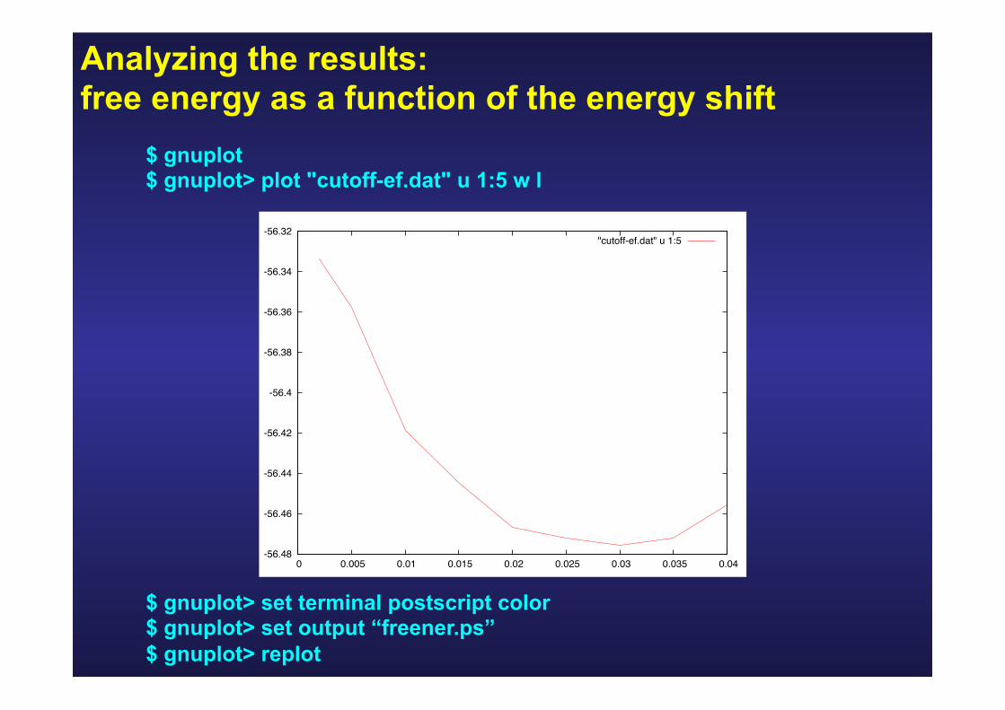
Analyzing the results: free energy as a function of the energy shift

$ gnuplot $ gnuplot> plot "cutoff-ef.dat" u 1:5 w l

$ gnuplot> set terminal postscript color $ gnuplot> set output “freener.ps” $ gnuplot> replot

-56.48

-56.46

-56.44

-56.42

-56.4

-56.38

-56.36

-56.34

-56.32

0 0.005 0.01 0.015 0.02 0.025 0.03 0.035 0.04

"cutoff-ef.dat" u 1:5

Analyzing the results: time per SCF step as a function of the energy shift

$ gnuplot $ gnuplot> plot "cutoff-ef.dat" u 1:6 w l

$ gnuplot> set terminal postscript color $ gnuplot> set output “timer.ps” $ gnuplot> replot

1

1.5

2

2.5

3

3.5

4

4.5

5

5.5

0 0.005 0.01 0.015 0.02 0.025 0.03 0.035 0.04

"cutoff-ef.dat" u 1:6