exercise topic: getting started with hec-geohms500 mb... · objectives: create a hec-hms model of...

1

George Mason University

Department of Civil, Environmental and Infrastructure Engineering

Dr. Celso Ferreira Prepared by Lora Baumgartner December 2015

Revised by Brian Ross July 2016

Exercise Topic: Getting started with HEC-GeoHMS ____________________________________________________________________________________________________________ Objectives: Create a HEC-HMS model of the George Mason University watershed using the GeoHMS toolbar in ArcMap.

a) Terrain Preprocessing

b) Generating a GeoHMS Project

c) Basin Processing

d) HMS Parameters

e) HMS Export

f) Running HMS

Challenges:

a) Find an appropriate CN table for the region and prepare a more elaborated land cover re-classification of the NLCD and create a CN look

up table. Repeat your analyses. How does that impact your design hydrograph?

b) After opening the GeoHMS file in HEC-HMS, what information is missing? Complete HMS set-up in order to run it. Change Metl model

to a SCS storm and use Fairfax County IDF curves to estimate a 100 yr design storm. Run HMS and plot the final hydrograph.

**Refer to the HEC-GeoHMS User Manual for definitions and context of the steps and tools in this tutorial, currently found at

http://www.hec.usace.army.mil/software/hec-geohms/documentation/HEC-GeoHMS_Users_Manual_4.2.pdf**

Tutorial DEM obtained from GMU Campus Lidar file (provided)

Versions used for this tutorial: HEC-GeoHMS 10.2, ArcMap 10.2.2 (Student), ArcCatalog 10.2.2

2

Prepare Project Workspace

1. Enable the “Hec-GeoHMS” toolbar under the Customize > Toolbars menu in ArcMap.

2. Select “Add Data” under the File > Add Data menu.

3

3. Locate the folder location of the

GMU Campus Lidar DEM.

4. Select the GMU DEM.

5. Click “Add”.

6. If ArcMap suggests pyramid-building at this point, click “Yes”.

7. Select “Add Data” under the File > Add Data menu.

4

8. Select “Topographic” or other

preferred base map.

9. Click “Add”.

10. Disable the DEM layer to fully view the basemap.

11. Zoom to the campus area, leaving a generous border around the campus perimeter.

5

12. Select “Data Frame Properties”

from the View menu.

13. Near the bottom of the dialog box, select “Clip to shape” from the Clip options drop-down menu.

14. Click “Specify Shape”.

15. Confirm that the “Current Visible Extent” radio button is selected.

16. Click “OK”. On the Data Frame Clipping dialog box.

17. Click “OK” to clip all data layers (DEM and basemap) to the applicable geographic area.

Clipping the data layers limits the amount of data in the project and speeds processing. However, be sure that the extents of the watershed are completely included after clipping.

18. Save As to save the new project.

6

Terrain Preprocessing These Terrain Preprocessing steps correlate with the Spatial Analyst-Hydrology functions performed in the ArcGIS tutorial.

1. Select “Fill Sinks” from the Preprocessing menu on the HEC-GeoHMS toolbar in ArcMap.

2. Confirm that the “Input DEM” field was auto-filled with the correct raw GMU DEM file.

3. Confirm that the output location is correct and note the name of the new layer. GeoHMS will auto-generate layer names for each preprocessing step. The layer names can be changed, but customized names will not be recognized in future GeoHMS steps and will require manual entry. For this tutorial, do not change the default (auto-generated) layer output names.

4. Click “OK”.

5. Observe visual changes to the model and click “Close”.

7

1. Select “Flow Direction” from the

Preprocessing menu on the HEC-

GeoHMS toolbar in ArcMap.

2. Confirm that the “Input Hydro

DEM” field was auto-filled with the

new Filled DEM layer.

6. Confirm that the output location is correct and note the name of the new layer.

3. Click “OK” to generate the new

layer.

4. Observe visual changes to the

model and click “Close”.

8

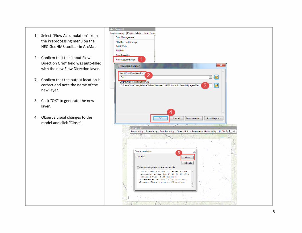
1. Select “Flow Accumulation” from

the Preprocessing menu on the

HEC-GeoHMS toolbar in ArcMap.

2. Confirm that the “Input Flow

Direction Grid” field was auto-filled

with the new Flow Direction layer.



layer.



9

1. Select “Stream Definition” from the




Accumulation Grid” field was auto-

filled with the new Flow

Accumulation layer.



layer.



10

1. Select “Stream Segmentation” from

the Preprocessing menu on the

HEC-GeoHMS toolbar in ArcMap.

2. Confirm that the “Input Stream

Grid” field was auto-filled with the

new Stream Definition layer.



layer.

5. Observe any changes to the model

and click “Close”.

11

1. Select “Catchment Grid

Delineation” from the





with the correct layer. Confirm

that the “Input Link Grid” field was

auto-filled with the New Stream

Segmentation layer.

3. Confirm that the output location is

correct and note the name of the

new layer.


layer.



12

1. Select “Catchment Polygon

Processing” from the Preprocessing

menu on the HEC-GeoHMS toolbar

in ArcMap.

2. Confirm that the “Input Catchment

Grid” field was auto-filled with the

new Catchment Delineation layer.



new layer.


layer.



13

1. Select “Drainage Line Processing”

from the Preprocessing menu on

the HEC-GeoHMS toolbar in

ArcMap.

2. Confirm that the “Input Stream

Link Grid” field was auto-filled with

the new Stream Segementation

layer. Confirm that the “Input Flow


with the correct layer.



new layer.


layer.

5. Observe any changes to the model

and click “Close”.

14

1. Select “Adjoint Catchment

Processing” from the Preprocessing

menu on the HEC-GeoHMS toolbar

in ArcMap.

2. Confirm that the “Input Drainage

Line” field was auto-filled with the

new Drainage Line layer. Confirm

that the “Input Catchment” field

was auto-filled with the correct

layer.



new layer.


layer.



15

When viewed in ArcCatalog, the project should appear similar to the image at right.

16

Generate a New Project

1. Select “Data Management” from the Project Setup menu on the GeoHMS toolbar in ArcMap.

2. Validate that all fields are auto-filled properly. Pay particular attention to the Raw DEM field, which should be populated by the original GMU Lidar DEM.

3. Click “OK”.

4. Select “Start New Project” from the Project Setup menu.

5. Note the names of the new Project Area and Point; click “OK”.

17

6. Assign a Project Name and Project

Description.

7. Confirm the save location.

8. Click “Okay”.

9. Review the steps listed in the dialog box and click “OK”.

10. On the left sidebar table of contents, uncheck all layer except for “Drainage Line” and “Basemap.

18

11. Zoom in to the main campus outlet

point just above Braddock Rd. A scale of 1:15 is recommended to provide optimum accuracy..

12. Click the Pushpin (“Add Project Point”) icon on the GeoHMS toolbar.

19

13. Hover directly over the drainage

line and click to place the outlet point exactly on the stream.

14. Note the name and description of the new Project Point and click “OK”.

15. Select “Generate Project” from the Project Setup menu.

16. When the Project has been generated, review the watershed area and click “Yes”.

20

17. Review the layers assigned to each

field for the project. Make any corrections, again paying special attention to the raw DEM.

18. Click “OK”.



21

Prepare Slope Grid in ArcMap This layer is a required input for additional GeoHMS processing.

1. At the top of the ArcMap screen, select “ArcToolbox” from the Geoprocessing menu.

2. Select “Slope” from the Spatial Analyst > Surface menu.

3. Select the Filled DEM layer for the GeoHMS project.

4. Click “Add”.

22



new layer.

6. Click “OK”.



23

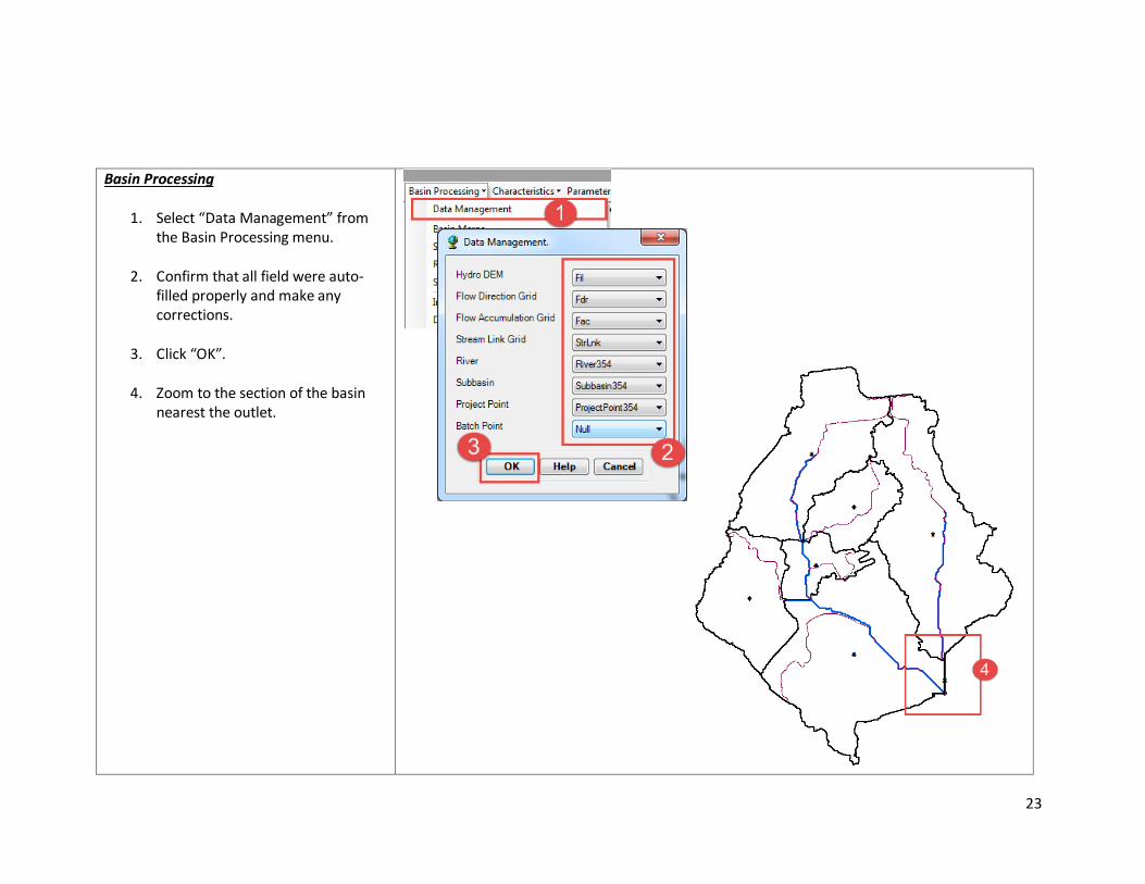
Basin Processing

1. Select “Data Management” from the Basin Processing menu.

2. Confirm that all field were auto-filled properly and make any corrections.

3. Click “OK”.

4. Zoom to the section of the basin nearest the outlet.

24

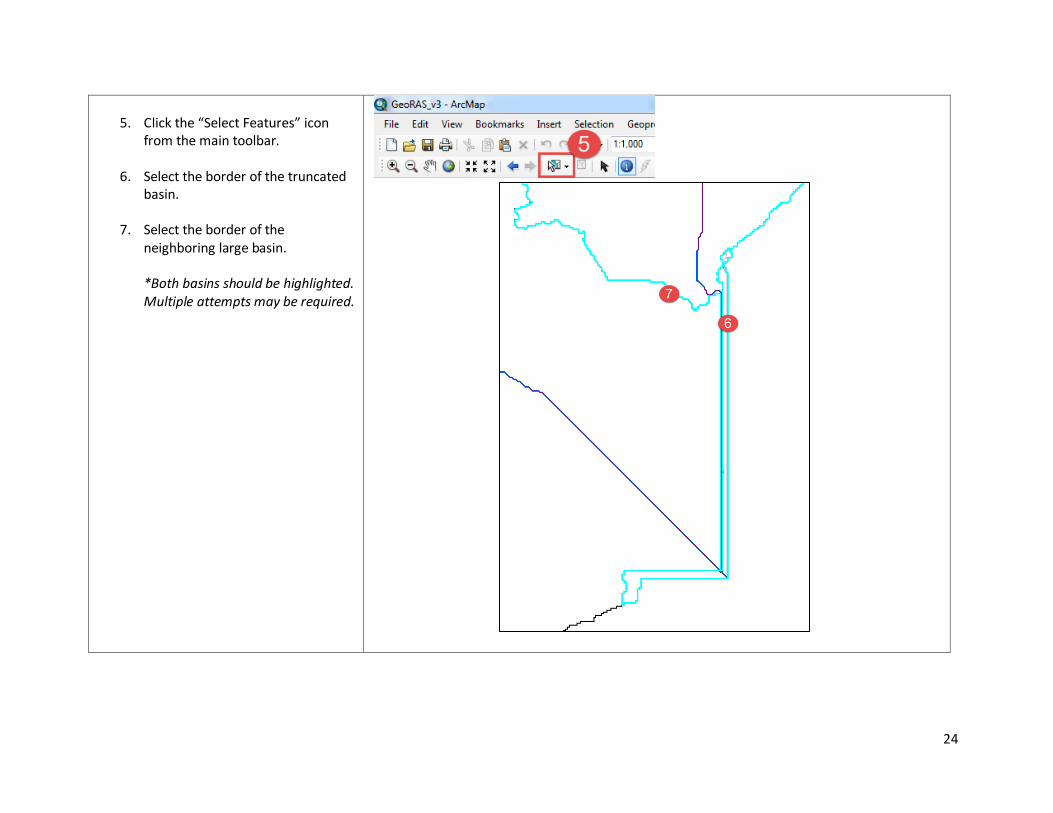
5. Click the “Select Features” icon

from the main toolbar.

6. Select the border of the truncated basin.

7. Select the border of the neighboring large basin. *Both basins should be highlighted. Multiple attempts may be required.

25

8. Select “Basin Merge” from the

Basin Processing menu.

9. Confirm that the crosshatched areas match the basins to be merge. Click “OK”.

26

Identify River and Subbasin Characteristics

1. Select “Data Management” from the Characteristics drop-down menu on the GeoHMS toolbar.

2. Confirm that all field were auto-filled properly and make any corrections.

3. Click “OK”.

27

1. Select “River Length” from the

Characteristics drop-down menu.

2. Input the new River layer.

3. Click “OK”.

4. Click “Close”.

5. To view the output of the River Length tool, right click on the River layer in the left sidebar and select “Open Attribute Table”. Note that a column named RivLen has been added.

28

1. Select “River Slope” from the


2. Input the RawDEM (original GMU Lidar DEM) and the River layers.

3. Click “OK”.


5. If there is an error due to a background exception, select “Geoprocessing Options” under the geoprocessing tab. Disable “background processing” by unchecking the “enable” box. Then, retry the river slope.

6. To view the output of the River Length tool, right click on the River layer in the left sidebar and select “Open Attribute Table”. Note that a column named Slp has been added.

29

1. Select “Basin Slope” from the


2. Input the Slope layers that was generated at the beginning of this section. Input the Subbasin layer.

3. Click “OK”.


5. To view the output of the Basin Slope tool, right click on the Subbasin layer in the left sidebar and select “Open Attribute Table”. Note that a column named BasinSlope has been added.

30

1. Select “Longest Flowpath” from the


2. Input the RawDEM (original GMU Lidar DEM) and the Flow Direction layers.

3. Click “OK”.


31

1. Select “Basin Centroid” from the


2. Confirm that the “Center of Gravity” method and the Subbasin layer are selected.

3. Click “OK”.

4. Note that centroid asterisks have been added to the project. Click “Close”.

32

1. Select “Centroid Elevation” from

the Characteristics drop-down menu.

2. Input the Raw DEM (original GMU Lidar DEM) and the Centroid layers.

3. Click “OK”.


5. To view the output of the Centroid Elevation tool, right click on the Centroid layer in the left sidebar and select “Open Attribute Table”. Note that a column named Elevation has been added.

33

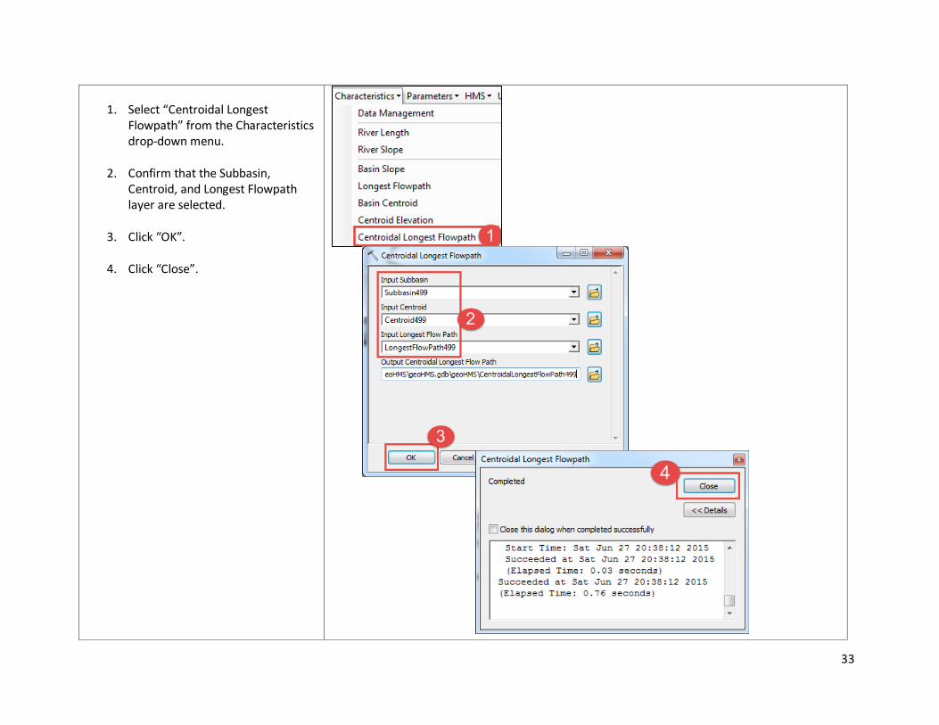
1. Select “Centroidal Longest

Flowpath” from the Characteristics drop-down menu.

2. Confirm that the Subbasin, Centroid, and Longest Flowpath layer are selected.

3. Click “OK”.


34

1. Select “Data Management” from

the Parameters drop-down menu.

2. Confirm that the auto-filled fields contain the correct layers. Several layers have not yet been generated and the associated fields will contain “null” values.

3. Click “OK”.

35

1. Select “Select HMS Processes” from

the Parameters drop-down menu.

2. Input the Subbasin River layers.

3. Choose “SCS” from the Subbasin – Loss Method drop-down menu.

4. Choose “SCS” from the Subbasin – Transform Method drop-down menu.

5. Choose “None” from the Subbasin – Baseflow Method.

6. Choose “Muskingum” from the River – Route Method drop-down menu.

7. Click “OK”.


9. To view the output of the Select HMS Processes tool for the Subbasin and River, right click on the Subbasin and River layers in the left sidebar and select “Open Attribute Table” for each. Note that columns have been added for the outputs of steps 3 through 6 above.

36

1. Select “River Auto Name” from the

Parameters drop-down menu.

2. Input the River layer.

3. Click “OK”.


5. To view the output of the River Auto Name tool, right click on the River layer in the left sidebar and select “Open Attribute Table.” Note that a column has been added for the output of the Auto Name tool.

37

1. Select “Basin Auto Name” from the


2. Input the Subbasin layer.

3. Click “OK”.


5. To view the output of the Basin Auto Name tool, right click on the Basin layer in the left sidebar and select “Open Attribute Table.” Note that a column has been added for the output of the Auto Name tool.

38

1. Add the provided curve number

grid to the project by selecting it in the File > Add Data menu.

2. Click “Add”.

3. Select “Subbasin Parameters from Raster” from the Parameters drop-down menu.

4. Input the Subbasin layer.

5. Input the Curve Number Grid.

6. Click “OK”.

39


8. To view the output of the Subbasin

Parameters from Raster tool, right click on the Subbasin layer in the left sidebar and select “Open Attribute Table”. Note that a column has been added for the output of steps 3 through 6 above.

40

1. Select “CN Lag” from the


2. Click “OK”.

3. To view the output of the CN Lag tool, right click on the Subbasin layer in the left sidebar and select “Open Attribute Table”. Note that a column has been added for the output of steps 1 through 3 above.

41

1. Select “Data Management” from

the HMS drop-down menu.

2. Confirm that all fields have been auto-filled with the proper layers.

3. Click “OK”.

42

1. Select “Map to HMS Units” from the

HMS drop-down menu.


3. Click “OK”.

4. Select English units.

5. Click “OK”.

43

1. Select “Check Data” from the HMS

drop-down menu.


3. Click “OK.

4. If data problems are found, click “Yes” to view.

5. It is common for a project point error to be generated.

6. Zoom to the project point (outlet) area. If the project point can be confirmed to lie directly on the River, disregard the Check Data Error.

44

1. Select “HMS Schematic” from the

HMS drop-down menu.


3. Click “OK.

4. Note that new visual representations have been added.

5. Click “OK”.

45

1. Select “HMS Legend” from the HMS

> Toggle Legend drop-down menu.

2. Note that HMS icons are shown.

46

1. Select “Add Coordinates” from the

HMS drop-down menu.


3. Click “OK”.

4. Click “OK” to accept 2-dimensional units.

5. Click “OK”.

47

1. Select “Prepare Data for Model

Export” from the HMS drop-down menu.


3. Click “OK”.

4. Click “OK” to accept 2-dimensional units.

5. Click “OK”.

48

1. Select “Background Shape File” from

the HMS drop-down menu.


3. Click “OK”.

4. Click “OK”.

49

1. Select “Basin Model File” from the

HMS drop-down menu.

2. Note the name and location of the HMS model.

3. Click “OK”.

50

1. Select “Specified Hyetograph” from

the HMS > Met Model File drop-down menu.


3. Click “OK”.

4. Click “OK”.

51

1. Select “Create HEC-HMS Project”

from the HMS drop-down menu.

2. Select the proper file location and file names of the newly-created basin and met models.

3. Name the Simulation Run 1.

4. Select 5-minute Time Intervals.

5. Click “OK”.

6. Confirm that all functions were successful.

7. Click “OK”.

Refer to the HEC-HMS tutorial for context of the project components being created during steps 1 through 5.

exercise topic: getting started with hec-geohms500 mb... · objectives: create a hec-hms model of...

Documents