1

Exercise 5. Building ArcGIS Tools using Python

GIS in Water Resources, Fall 2014

Prepared by Anthony Castronova

Purpose

The purpose of this exercise is to illustrate how to build ArcGIS tools using the Python

programming language. Python is included with ArcGIS. This exercise will guide you

through the processes of collecting data via ArcGIS services, creating and running an

ArcGIS Python script and creating a model builder tool interface for the script. The

purpose of the ArcGIS tool is to provide you with an example of how to manipulate

shapefiles, iterate over raster datasets, execute native ArcGIS tools, as well as define

ArcGIS tool parameters. Overall, it will provide guidance on how to build your own

ArcGIS tool. The tool outlined in this exercise will trace a user-defined point

downstream until it hits a watershed outlet.

Learning Objectives

To be able to create and run a python script using ArcGIS functions in the arcpy

library

To be able to configure a user interface for an ArcGIS python script

To be able to split a problem into individual steps and program these steps into a

Python script that executes them in sequence to solve the problem

Computer and Data Requirements

To carry out this exercise, you need to have a computer that runs ArcGIS 10.2 or higher

and includes the Spatial Analyst extension. No data is required to start this exercise. All

the necessary data will be extracted from ArcGIS.com services. To use these services you

need an ArcGIS.com account that has been linked to an ArcGIS license.

This exercise is divided into the following activities:

1. Data Collection

2. Developing a python script

3. Developing a toolbox interface for a python script

2

Part 1: Data Collection

This section of the exercise uses ArcGIS.com tools to delineate a watershed and extract

the DEM as you have done in previous exercises. This gets us the data for using in the

model building and python scripting part that follows

Open ArcMap.

Connect to the ArcGIS hydrology server http://hydro.arcgis.com/arcgis. We will use this

to delineate a watershed.

If added correctly, you should see the following tools listed in ArcCatalog.

Next, add a connection to the ArcGIS landscape1 server. We will use this web service to

download and visualize National Hydrography Dataset (version 2) rivers. Use

https://landscape1.arcgis.com/arcgis/services as the URL. If added correctly, you will

see long list of datasets under the landscape1 service in ArcCatalog.

3

Finally, connect to the ArcGIS elevation web service. This will be used to downloading

elevation data for the exercise. Use http://elevation.arcgis.com/arcgis/services as the

URL. If added correctly, you will see a short list of tools and data available under the

elevation service in ArcCatalog.

Add some template data so that we can zoom into the location that we would like to

download data. Select the Add Data button:

4

Navigate to the ArcGIS template data directory (C:\Program Files

(x86)\ArcGIS\Desktop10.2\TemplateData\TemplateData.gdb\USA) and add US cities,

interstates, and states.

The map should now look like this:

5

Zoom into Logan, UT. Use the Identify tool to determine which of these dots is Logan.

This will give us an idea of where we are, before we start loading ArcGIS web service

datasets.

Add the NHDPlus (version 2) data set from the landscape1.arcgis.com web service.

We are only interested in the stream data, so turn off all NHD layers except Streams.

This will help speed up the data load time. The layers in your table of contents should

look like this:

6

Now that we have the NHD rivers loaded, we can zoom into Right Hand Fork.

7

To delineate a watershed at Right Hand Fork, we will use the ArcGIS online watershed

delineation tool. Double click on the ArcGIS server watershed tool.

Select an input point near the outlet of Right Hand Fork (see green dot on map). Don’t

get too close to the Logan river (downstream), or the delineation tool will snap the

outlet to the wrong reach. To ensure that this does not happen, you may have to adjust

the snap distance (try 100 meters)

This operation will result in the Right Hand Fork watershed. Go ahead and turn off all

unnecessary layers and change the watershed color to something more meaningful.

Export the in-memory watershed data to create a new shapefile, called watershed.shp.

8

We will use this new watershed.shp file in the following step to extract elevation data

over the watershed.

Add NED30m elevation from the elevation.arcgis.com server.

9

Next we want to extract the elevation data within the boundary of our watershed. This

will make future data processing faster since we will be using a small subset of the

national elevation dataset. In addition, this file will be stored locally so we won’t need

an Internet connection to perform our processing tasks. To do this, open the search

menu and enter “Extract”. Make sure to choose the search by “Tools” option above the

search textbox. This will limit the search results ArcGIS tools. Since we are dealing with

elevation data from an ArcGIS server, we want to select the “Extract Data (server)” tool.

10

Select the NED 30m elevation raster as the layer to clip. The Area of Interest that will be

used to extract the data (i.e. cookie cutter) should be the watershed that you delineated

in previous steps. Leave the default options for Feature Format, Raster Format, Spatial

Reference, and Custom Spatial Reference Folder. Specify an output ZIP file where the

extracted data will be saved.

Open Windows Explorer and navigate to the directory of your output ZIP. Extract the

contents, and you should now have an elevation dataset that covers only the watershed

area.

This is a good time to change the projection of our data frame to match the coordinate system of this elevation data. Also be sure to change the map units to be consistent with the units of the coordinate system.

11

Part 2: Developing a python script

The goal of our scripting tool is to trace any point within the watershed downstream to

the watershed outlet. This can later be modified to provide statistics regarding the flow

path. This example will demonstrate (1) how ArcGIS tools can be used to create a

custom model, (2) how to include custom data processing and functionality, and (3) how

to build the ArcGIS tool interface for a custom tool.

An effective way to learn programming is by example. ArcGIS models built using model

builder can be exported as python scripts that serve as examples that show how ArcGIS

functions are used in python. The exported file also serves as a template for you to edit

to develop the tool you want to use. The strategy will be to

(1) create a model using model builder

(2) export it as a python script

(3) set the inputs and outputs and run the script

(4) make incremental changes to the script running after each change to ensure that

the script still works

Note that developing Python scripts for ArcGIS is hard and sometimes you encounter

errors that appear insurmountable. If this should happen to you do not waste too much

time on this. A complete set of scripts from this exercise have been posted in

http://www.neng.usu.edu/cee/faculty/dtarb/giswr/2014/Ex5Scripts.zip. These are

named trace1.py, trace2.py … up to trace5.py then the final script is trace.py. The

exercise below has check points and indicates which script applies for work up to that

point. If you get stuck feel free to go to the next check point and start with the

corresponding script and move on. The questions at the end can be done with small

changes to the final script trace.py.

Activate the ArcToolbox by clicking . Create a new toolbox by right clicking inside

the window and selecting Add Toolbox from the context menu. This will open a dialog

for you to search for an existing toolbox. Instead, navigate to any directory that you like

and select the create New Toolbox button in the top right corner .

12

After creating your toolbox (i.e. Exercise 5), right click on it and select New -> Model.

You will end up with an empty model. Drag and drop the Fill tool onto the canvas, along

with the clipped elevation raster.

From the menu, select Model -> Export -> To Python Script and save the script with the

name trace.py. (Named trace.py because that is the ultimate goal of our work)

13

Close the ArcMap model. From the Windows Explorer open the exported Python file to

view the code that was written for us by ArcGIS. We can do this using the IDLE

application by simple right clicking on the file and selecting “Edit with IDLE.”

You should see the following Python Idle editing window.

14

Although cryptic to a reader new to Python this is readable. Comment lines are

preceded by # and are not run. You can see the line to import the arcpy library that tells

the script to use ArcGIS functions. Then there is the line to use the spatial analyst

extension, two lines to specify the input variables. These are files on your disk. Then

there is the command to run the Fill function.

Lets run this script. Select Run -> Run Module

The Python Shell should open and your script will run. There is no output from this

script to the shell so your only indication that it is done is the appearance of the third

>>> prompt.

15

Note the following lines in the script.

These define ned30m and Fill_ned30m2 as variables with values to the right. Then the

line below executes the Fill function with these as input and output. If your script ran

correctly you can look in the destination location

"C:\users\dtarb\Documents\ArcGIS\Default.gdb" above and see the result.

You may get an error due to input files not being correct. If you get the error do not

worry about it as our next step will be to change the location of inputs and outputs.

Note that in Python \ is an "escape" character so to get folder paths that include it you

need double \\. Alternatively you can use "/".

Now lets modify this code so that the variable names and files used make a bit more

sense

Change the file to the following and rerun it

16

Note the F5 shortcut for running this script that is handy as you will be doing this a lot.

Click OK when prompted to save the file.

Note that now the output file "Fill" is produced in the folder you have designated and

that the script prints 'done' when it is finished. Congratulations! You have just modified

a script and been able to execute it. This is a small but important step as it establishes

your capability to change and execute ArcGIS functions from a script file. You are now

programming and limited only by your creativity in the programming lines you can

write.

The script to this point is trace1.py in

http://www.neng.usu.edu/cee/faculty/dtarb/giswr/2014/Ex5Scripts.zip.

Now lets edit the code to add additional functionality as follows. This imports numpy,

math, json, and os libraries that we will need later as well as env and sa classes from the

arcpy library.

17

Run this code and see what kind of output we get. If the script ran successfully, we

should have a new raster called fill that can be opened in ArcMap. Note: the original

script used the gp.Fill_sa tool whereas the documentation states that we should use the

arcpy.sa.Fill tool. If you encounter this, I suggest that you use the tools outlined in the

ArcGIS documentation.

Note that the line env.overwriteOutput = True sets the script to overwrite any output

files that already exist. This is useful when repeatedly running a script to incrementally

develop it as we are doing here. However if you leave one of the files loaded into

ArcMap while you do this you may get an error that corrupts the raster file. If this

happens you need to delete the raster file to get it working again.

Next, lets add to our script the function to calculate flow direction. To determine the

syntax for this operation we can google “ArcGIS Flow Direction”:

http://help.arcgis.com/en/arcgisdesktop/10.0/help/index.html#//009z00000052000000

.htm

18

The script to this point is trace2.py in

http://www.neng.usu.edu/cee/faculty/dtarb/giswr/2014/Ex5Scripts.zip.

Notice that the output from the fill operation was not Saved, but it can still be used in

the following step! This is because it is saved temporarily in memory. We can utilize

this feature to “hide” intermediary processing outputs. Lets look at the output from the

flow direction process.

19

Now that we have some of the basic raster processing done, lets create a point that can

be traced to the outlet. This will be hardcoded for now, but we can change it to a user

input later.

20

In order to relate this point coordinate with the raster data, we need to do two things:

(1) represent the raster grids as arrays of data, and (2) convert the x,y point coordinate

into array indices. To convert the raster grids (i.e. fill and fdr) into arrays, we use the

numpy library, specifically RastertoNumPyArray.

21

Examine the value of the fdr value to see what it looks like. You can do this by typing

the object name fdr in the Python Shell after the script has been run.

22

It looks like there are lots of 0’s, however this is just because we are seeing a small

subset of the data. In fact most of the cells near the edge of the raster will be zero. Lets

look at some values elsewhere:

Before we do anymore processing of the raster data, we need to extract some metadata

that will enable us to loop over the raster cells. The numpy arrays only contain raster

values, so we will need to use the ArcGIS Raster type to retrieve this information.

23

We can transform our point coordinates into array indices, now that we have the upper

left (x,y), cell width, and cell height. This will enable us to access the raster value of the

cell associated with our point.

24

Lets see where our point lives in the raster array (again, this is easy to do using the IDLE

Python Shell). Your coordinates may be different than those below due to the extent of

your watershed raster.

Now we are ready to start moving our point around within the raster. Specifically, we

want to move our point from its current location (62,210) to the next downstream cell.

In order to accomplish this, we need to add a function at the top of our script to check

the value of our flow direction grid and move the point accordingly. Place this function

right below the import statements.

25

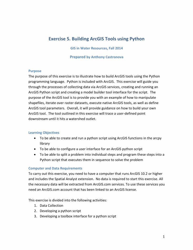
This function takes in three arguments: fdr (flow direction array), row (current row

index), col (current col index). The first thing that it does is extract the value of the flow

direction grid at the current (row, col) location. It then checks this value against all the

possible flow direction combinations to determine the next downstream neighbor. It

increments the current (row, col) pair and returns the result.

Lets pass in the coordinates of our point and see which direction our cell will flow.

26

We can verify this by loading the flow direction raster into ArcMap.

Use the Go To XY Tool on the Tools Menu

Set the units to Meters

Zoom in and look at the value of fdr at the selected location (using the coordinates of

our point)

27

Note the fdr value of 1 which corresponds to a flow direction the east consistent with

the direction that the function is moving the point

Lets modify our code to repeat this process until the point moves beyond the extent of

our raster grid (e.g. through the outlet). In order do so, we need to create a loop that

will run until the value at location (r,c) is equal to NoDATA (in this case 0).

28

This loop will continue to run while the value of z does not equal 0 (i.e. no data value).

When a value of z=0 is encountered the while statement will be false and the loop will

stop. This code will thus move the point (r,c) to its downstream neighbor, and continue

to do so until we reach the edge of the DEM. Unfortunately, we have no output to

visualize. Let's save these points in a list and then create a shapefile that we can

visualize in ArcMap.

29

The script to this point is trace3.py in

http://www.neng.usu.edu/cee/faculty/dtarb/giswr/2014/Ex5Scripts.zip.

To visualize our output in ArcMap, add the coords.txt file to an ArcMap document.

Right click on it and select Display X,Y data. Choose Field1 as the X field and Field 2 as

the Y field. You can also symbolize these points by their elevation, Field 3

30

Since point text file is not an ideal output, lets format it as a PolyLine Shapefile,

http://help.arcgis.com/en/arcgisdesktop/10.0/help/index.html#//00170000002p00000

0. In the code snippet below, we first create the polyline feature class that will hold our

results. Next we loop over our coordinates are create line segments between each pair.

These line segments are then added to the feature class as a polyline. Add the

following code to replace the 3 lines that create coords.txt.

31

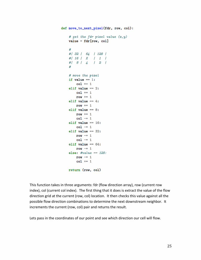
This produces an output Shapefile called path.shp. We can view this in ArcMap:

32

The script to this point is trace4.py in

http://www.neng.usu.edu/cee/faculty/dtarb/giswr/2014/Ex5Scripts.zip.

Wow! Now we have a function that can trace a path from an arbitrary point to the edge

of the DEM. Pretty impressive. This is the functionality we set out to achieve. However

it is not very easy to use. The next section will build an interface.

Part3: Developing toolbox interface

First create a symbolic layer, which will be used in the next step, to assign a theme to

one of our inputs. This will also allow us to incorporate an interactive point input

selection feature. To do this, right click inside ArcCatalog and select New -> Shapefile.

33

Set a name for this file (e.g. my_point.shp) and set the feature type to Point. Change

the symbology of this point however you would like. Lastly, right click on the

my_point.shp in the Table of Contents and select Save as Layer File.

34

Now let's add our new script to the ArcGIS toolbox, so that we can run it like any other

tool. Right click on your toolbox (e.g. Exercise5) and select Add -> Script.

Give it a name and a label. Note that I also checked Store relative path names so that if I

put the toolbox and script in a different location they will work together. Then select

next. Specify the location of the python file and select next.

35

At the next dialog add input parameters. The first input parameter will be the start

point of the trace operation. Specify a Display Name (such as StartPoint) and set the

datatype to FeatureSet. Next select the Schema property and set its value to the

symbology layer that we created in the previous step. (e.g. symbology.lyr)

Next add the parameter for Elevation (input).

36

Next add the parameter for Fill (output) and Flow Direction (output).

Lastly add Path as a shapefile (output). When all five parameters are correctly set click

Finish.

37

If you do not get these settings right the first time you can get back to these controls by

right clicking on the script in the toolbox and selecting properties then the parameters

tab.

Now we need to add some code to our python script to utilize these parameters. We

use the arcpy.GetParameter(index) function to grab user inputs from the ArcGIS UI.

The following snippet gets the first parameter (i.e. Start Point) as a feature set, and

extracts the (x,y) coordinates. This code should be placed directly under the

move_to_next_pixel(fdr, row, col) function.

38

Next, let's add some code to get the rest of our inputs and outputs:

Since we are getting these parameters from ArcGIS, we need to remove our old

hardcoded paths. We should also add some messages, since our print statements will

not appear anywhere. The final script should look like this:

39

40

41

With these changes to our python script, we should be able to successfully run our tool

from the ArcGIS toolbox.

42

Notice that our output messages appear in the standard ArcGIS output dialog.

43

Our end result is a PolyLine shapefile that shows that path water would flow (using D8

flow direction) to the watershed outlet.

The complete script is trace.py in

http://www.neng.usu.edu/cee/faculty/dtarb/giswr/2014/Ex5Scripts.zip and the script

tool interface is in Exercise5.tbx in this zip file. If you have trouble developing your own

script you may use these in answering the questions below though you will need to

introduce small modifications to answer some of the questions. You will need to add

Exercise5.tbx to your map document and keep trace.py in the same folder. I have found

44

that unless after doing this I save the document then close and reopen ArcMap, I get an

error.

Homework Questions

1. Prepare a layout showing the elevation grid and two trace downstream paths.

Include a scale and label the length of each trace in the layout.

2. Write statements to determine and print the value of the flow direction array at

location with map coordinates (-1214936, 309638). You will need to determine

the array coordinates corresponding to this and then look up and print the value

of the fdr array at this location. Give the code you changed to achieve this and

show a screen shot of your output, either from print statements to the shell or

arcpy.Addmessage statements to the ArcGIS output.

3. Modify the script to compute and print out the length of the flow path being

traced. Give the code you changed to achieve this and show a screen shot of

your output.

4. Explain (without doing) how could you modify this code to determine the longest

flow path in the entire watershed?