executive compensation, financial constraint and product...
TRANSCRIPT

Executive Compensation, Financial Constraintand Product Market Strategies
Jaideep Chowdhury∗
January 17, 2012
Abstract
In this paper, we provide an additional factor that can explain afirm’s product market decisions. Managerial compensation can strate-gically affect a firm’s product market decisions. Higher variable com-pensation provides incentives for a manager to act more aggressivelyin the product market. We develop a theoretical model to examinehow the product market, managerial compensation and financial con-straints are interlinked in a Cournot duopoly setup. Empirically, wereport that the firm’s behavior in the product market can be explainedby the variable component of the managerial compensation structure.We also document that the financially constrained firms are more ag-gressive in the product market. Further, we report that the financiallyconstrained firms offer higher variable compensation as performanceincentives in the compensation package of their managers. This maybe an explanation as to why financially constrained firms are moreaggressive in the product market.
Keywords : Product Markets,Capital Markets, Financial Constraints, Ex-ecutive Compensation
1 Introduction
What are the different factors which can affect the product market be-havior of the firms? The question is important because strong performance
∗Department of Finance and Business Law, James Madison University, Harrisonburg,Virginia 22807, USA. Email: [email protected]
1

in the product market helps the firms not only in the stock market but alsoin the capital market. The literature on product market and financial marketinteraction is concentrated on how debt financing affects firm performance.In this paper, we introduce a new factor managerial compensation whichaffect firms’ performance in the product market. We also document thatthe financially constrained firms are more aggressive in the product markets.Further, we report that the financially constrained firms offer higher perfor-mance incentives in the compensation package of their managers which maybe an explanation as to why financially constrained firms are more aggressivein the product market.
Brander and Lewis (1986), Maksimovic (1988) and Hendel (1996) arguethat debt financing leads to more aggressive behavior in the product marketbecause of ‘risk shifting’ . The firm managers cater to the equity holders.They engage in riskier projects and act aggressively in the output markets.Glazer(1994) and Chevalier and Scharfstein (1996) believe that firms behaveless aggressively due to debt financing. They argue that ex-ante, debt financ-ing increases the probability of bankruptcy. If the firm faces high liquidationcosts and high bankruptcy costs, then the firm should behave less aggressivelyin the output market, i.e., by avoiding risky output market strategies. Weadd to the literature by introducing a new factor managerial compensationwhich may affect the product market behavior of the firms. We develop atheoretical model and then test empirically to show that the variable compo-nent of the managerial compensation positively affect the industry adjustedsales growth of the firms.
We derive optimal compensation contracts for the managers of the twofirms in a Cournot duopoly setup. The optimal compensation contract ofa manager is positively dependent on the value of the firm which, in turn,depends on the equilibrium output of the firm. This compensation structureprovides incentive to the manager to act more aggressively in the productmarket in order to secure higher equilibrium output. Following Aggarwal andSamwick (1999), we decompose CEO compensation into three components,flow compensation, change in the value of the stock holding and changein the value of stock options. We provide evidence that product marketaggressiveness can be explained by the different components of managerialcompensation after we control for endogenity problems. Industry adjustedsales growth is used as the proxy for aggressiveness in the product marketfollowing Campello(2003), Campello and Fluck(2004) and Opler and Tit-man(1994). Further, short run bonus, defined as ratio of bonus to totalcurrent compensation, explains industry adjusted sales growth which con-firms our intuition that incentive based compensations like short run bonusprovides incentives for the managers to be more aggressive in the product
2

market.We consider a Cournot duopoly setup. Both the firms raise capital from
the external capital market. The degree of financial constraint of a firm is de-pendent on how high is the cost of external capital for the firm. Both the firmsengage in risky and aggressive product market strategies like more spendingin advertisement, more research and development for increasing the equilib-rium output. But engaging in riskier projects involve higher probability ofbankruptcy and liquidation. A firm weighs the costs of acting aggressivelyagainst the benefits of aggressive product market behavior. Without loss ofgenerality, we assume that firm 2 is financially constrained, has higher costof capital which results in higher marginal cost of production as compared tofirm 1. Higher marginal cost of production leads to decrease in equilibriumoutput and profit for firm 2. When the degree of product differentiationis sufficiently high, the higher cost firm, firm 2, can act more aggressivelyand produce more in order to compensate for the higher cost of productionit faces. The first (second) effect decreases(increases) the amount of out-put produced. Which effect dominates depends on the extent to which firm2’s product is different from firm 1’s product. Theoretically we concludethat when the degree of product differentiation is sufficiently high, the morefinancially constrained firm acts more aggressively in the output markets.Further, we document empirically that more financially constrained firmsare more aggressive in the output markets compared to the less financiallyconstrained firms.
We report that the shares owned by the CEO, the change in the valueof stock option of the CEO, the total compensation of the CEO and bonusas a percentage of total current compensation are higher for more financiallyconstrained firms. Further, these are the same variables which are also thedeterminants of industry adjusted sales growth of a firm, our proxy for prod-uct market aggressiveness. This suggests that the difference in the productmarket aggressiveness between the more financially constrained firms andless financially constrained firms can be attributed to the differences in thecomponents of managerial compensation.
It should be noted that the theoretical model is not tested per se. Thisis the first limitation of the paper. Most of the assumptions made in thetheoretical model are too simple to be realistic. For example, the assumptionof constant marginal cost of production and linear demand function are madefor obtaining closed form solutions. But these assumptions are common intheoretical models. The theoretical model provides some justification for theempirical results we document in section 5. The theoretical model also serveto provide economic intuition to the empirical results. Another limitation ofthis paper is the use of industry adjusted sales growth of a firm as a measure of
3

product market aggressiveness of the firm. Ideally one should use productionlevel data to measure aggressive product market behavior of a firm. The lackof reliable plant level production data forces us to use industry adjusted salesgrowth of a firm as a measure of product market aggressiveness of the firm.This measure of aggressiveness of the firm has been used in several recentpapers such as Campello(2003)and Campello and Fluck(2004).
This paper contributes to three different strands of the literature. First,this paper contributes to the product market and financial market interac-tion literature. We provide an alternative explanation of product marketaggressiveness based on managerial compensation. This paper is the firstpaper to our knowledge to test if the product market aggressiveness can beexplained by the executive compensation structure. This paper shows empir-ically that short run bonus, managerial stock holding, change in the value ofstock options, total compensation and change in the value of stock holdingscan explain the product market behavior of the firms. Second, this papercontributes to the executive compensation literature. We document thatthe executive compensation structure is different for financially constrainedfirms. We document that more financially constrained firms’ managers havea higher percentage of bonus in total current compensation, higher stockownership, higher change in stock options and higher total compensation.To my knowledge there is only one other paper which deals with executivecompensation of the financially constrained firms. Wang (2005) shows thatthe CEO pay performance sensitivities are higher for financially constrainedfirms where performance is measured in terms of stock returns. She alsoreports that the total compensation packages of CEOs of financially con-strained firms are higher as compared to less financially constrained firms.The third stand of literature where we add to the body of knowledge is theliterature on financially constrained firms. Papers in this literature have sug-gested that financially constrained firms are more riskier firms because theyundertake riskier projects. We document that the financially constrainedfirms are more aggressive in the product market. This is the first paper inour knowledge which investigates the product market strategies of the finan-cially constrained firms. We conclude that the financially constrained firmsare more aggressive in the product market because the compensation struc-ture of these firms is more incentive oriented which encourages the managersto be more aggressive in the product market.
The paper is organized as follows. In section 2, I present a theoreticalmodel. In section 3, I develop my hypothesis based on the model in section 2.In section 4, I describe my data and methodology. In section 5, I documentmy results. In section 6, I conclude the paper.
4

2 A Theoretical Model
In this section, we present a theoretical model linking the financial con-straints with managerial compensation and product markets. Let us considera Cournot duopoly setup. Without loss of generality, let us assume that firm2 is more financially constrained than firm 1.
2.1 Definition of Financial Constraint
If a firm is financially unconstrained, the cost of internal capital and thecost of external capital should be the same. Any wedge between the cost ofinternal capital and the cost of external capital is a measure of the degreeof financial constraint. The cost of capital of firm 1 is r whereas the costof capital of firm 2 is r+d, where d is the extra cost of capital the morefinancially constrained firm 2 faces. The higher is the degree of financialconstraint, the higher is the value of parameter d.
2.2 The Two Stage Game
In this section, the manager of a firm i treats the wage contract as exoge-nous. The wage contract is given by
wi = αi + βiV1/3i , i = 1, 2. (1)
αi and βi are exogenous to the manager’s decision making process. Vi isthe equity value of the firm.1
2.2.1 The Set-Up
The two firms who engage in a Cournot duopoly game to maximize theirvalues. The manager of each firm chooses her effort and firm output.
In the first stage, the manager chooses her effort. Effort is unobservableto the equity holders and debt holders. The equity holders design a contractto ensure that the interest of the manager is aligned with that of the equityholders. This is done in order to tackle the agency problem between themanager and the equity holders. The managerial wage is composed of twoparts. The first component is αi which is the fixed component of managerialwage. The second component is βiV
1/3i , which is the variable component
of the compensation structure. This compensation structure is reasonable
1The wage contract is dependent on V1/3i instead of Vi in order to obtain a closed form
solution.
5

because in real world, manager’s compensation has a fixed component whichconsists of the salary and a variable component, which consists of bonus,perks and options granted.
The manager decides on two things: How much effort to put and howmuch output to produce. In the first stage, the manager maximizes herutility by choosing her effort. The managerial utility is given by
Ui = wi −e2i2, i = 1, 2. (2)
As manager’s variable wage depends on the value of the firm, the managerhas the incentive to maximize the value of the firm by putting in more effort.But putting in more effort is a disutility for the manager which is representedby the second term of equation 2.
There is an inverse market demand of the affine-linear form
pi = θ + ei + zi − qi − λqj (3)
where λ is the degree of product differentiation, θ > c is a positive constantand z is a random parameter, which represents the state of the nature. Wefurther assume that z is uniformly distributed on a non-degenerate interval[z, z] with constant density {
z ∈ [z, z]f(z) = 1
z−z(4)
If the manager puts more effort, the price increases leading to an increasein revenue. If the state of the nature improves, the firm can charge a higherprice and increase revenue. The equity holders, the debt holders and therest of the world cannot distinguish if the increase in revenue occurred dueto increase in manager’s effort or due to the improvement in the state of thenature, which is random. So the outside world cannot distinguish between eiand zi. If there is a reduction in firm revenue, the outside world cannot knowif the manager did not put in enough effort leading to a fall in demand orif the state of nature was bad. This creates an opportunity for the managerto act in her self-interest which is the reason for the existence of a principleagent problem between the manager and the equity holders of the firm. Thecompensation structure of the manager is aligned with the equity value ofthe firm in order to mitigate the agency problem between the equity holdersand the manager.
In the second stage, the manager of the firm chooses output to maximizethe equity value of the firm. The firm raises money from the debt holder tofund its project.
6

We assume absence of exogenous debt (for simplicity), zero fixed, set-upor sunk costs, and marginal cost of production c ≥ 0. We further assumethat the firm issues debt to finance its operating cost so that it will have debtequal to
D = cq
Thus there is an direct linkage between the financial decision and the outputdecision.
Switching state of nature, z is defined as that state of nature at whichthe revenue of a firm is just enough to pay off its debt and interest on debt.r is the rate of interest on debt. For firm 1:
(1 + r)D = R1(qi, qj, z),
(1 + r)cq1 = [θ + e1 + z1 − q1 − λq2]q1,
z1 = −[θ + e1 − (1 + r)c− q1 − λq2]. (4a)
For firm 2,
z2 = −[θ + e2 − (1 + r + d)c− q2 − λq1]. (4b)
This game is solved by backward induction. In the second stage, themanager of a firm engages in Cournot duopoly game with the other firm tomaximize the value of her firm and obtain the optimal value of q in termsof managerial effort. In the first stage, the managers of each firm choosetheir efforts simultaneously to maximize their utilities. Optimal efforts areobtained in terms of wage contract parameters αi, βi.
2.2.2 The Second Stage
Then with limited liability, a firm’s manager maximizes∫ z
z
[Ri(z; qi, q−i)−Di]f(z)dz,
For firm 1;
maxq1
V1 =
∫ z
z1
[[θ + e1 + z1 − q1 − λq2]q1 − (1 + r)cq1]f(z)dz. (5a)
For firm 2;
maxq2
V2 =
∫ z
z2
[[θ + e2 + z2 − q2 − λq1]q2 − (1 + r + d)cq2]f(z)dz. (5b)
7

It can be shown that thevalue of the firms are
V ∗1 =(q∗1)3
z(6a)
V ∗2 =(q∗2)3
z(6b)
where
q∗1 =z + θ + e1 − (1 + r)c− λ
3[z + θ + e2 − (1 + r + d)c]
(3− λ2
3)
(7a)
and
q∗2 =z + θ + e2 − (1 + r + d)c− λ
3[z + θ + e1 − (1 + r)c]
(3− λ2
3)
. (7b)
2.2.3 The First Stage
In stage 1, the manager of each firm chooses her effort simultaneouslywith the manager of the other firm to maximize her own utility:
maxei
Ui = wi −e2i2, i = 1, 2,
maxei
Ui = αi + βi(V∗i )
13 − e2i
2, i = 1, 2, (8)
where (V ∗i )13 is given by equation 6. Solving for ei, we get,
e∗i =βi
(z)13 (3− λ2
3), i = 1, 2. (8a)
We assume
3− λ2
3> 0. (A1)
Justification for this assumption is that in reality, the pay performance sen-sitivity βi is always positive. It does not make sense to have βi as negative.If 3− λ2
3< 0, then β < 0 for effort to be positive.
Individual rationality constraint suggests that the utility of an individualmanager must be greater than or equal to the reservation utility prevailingin the market. So
Ui ≥ U.
8

We assume that the labor market for managers is perfectly competitive whichimplies that a manager receives only the reservation utility. As a result,
U = αi + βiV1/3i − e2i
2, i = 1, 2.
Putting value of αi in the wage equation, we get,
wi = U +e2i2, i = 1, 2.
Putting the value of ei from equation (8a), the compensation contract ofthe manager is given by
wi = U +β2i
2(z)23 (3− λ2
3)2, i = 1, 2. (9)
The equilibrium outputs are given by
q∗1 =
z + θ + β1
(z)13 (3−λ2
3)− (1 + r)c− λ
3[z + θ + β2
(z)13 (3−λ2
3)− (1 + r + d)c]
(3− λ2
3)
(10a)and
q∗2 =
z + θ + β2
(z)13 (3−λ2
3)− (1 + r + d)c− λ
3[z + θ + β1
(z)13 (3−λ2
3)− (1 + r)c]
(3− λ2
3)
.
(10b)βi, i = 1, 2, are exogenous. Equilibrium outputs q∗1 and q∗2 depend on the
values of the parameters βi, i = 1, 2. βi, i = 1, 2, can be interpreted as thepercentage of short term variable compensation in total current compensa-tion. βi, i = 1, 2, can also be interpreted as the pay performance sensitivityof firm i.
2.2.4 Proposition 1
The more is the percentage of variable compensation in the total com-pensation of the manager of a firm, the more aggressive is the firm in theproduct market compared to its rival.
In Appendix A1, we show
dq∗2dβ2− dq∗1dβ2
> 0
9

Intuition: The compensation contract of the manager of firm 2 is givenby equation (1), wi = αi + βiV
1/3i . Equity value of a firm depends on its
output as given by equation (6). An increase in the value of the parameterβ2 implies more incentive to the manager of firm 2 to increase the value offirm 2 and hence increase firm 2 outputs. As this set-up is a Cournot duopoly,the output of rival firm, firm 1, decreases when firm 2 increases its output.
This illustrates why the compensation contract should play an activerole in the output market strategies. The variable portion of managerialcompensation is linked with the value of the firm, which crucially dependson the output of the firm. So an increase in the pay performance sensitivity,captured by the parameter β, (which can also be interpreted as the percentageof variable pay in total salary) provides incentive to the manager to act moreaggressively in the output markets.
Up to now, we have assumed that the compensation contract is exoge-nously given and the manager cannot affect the compensation structure.Specifically, we have assumed that the manager’s decisions cannot affect thevalues of α and β. This is too simplistic an assumption. The manager de-cides what should be the output which, in turn, determines the equity valueof the firm. The equity holder maximizes the net equity value of the firm bychoosing values of α and β. Her maximization problem is given by
maxαi,βi
V neti = Vi − wi
If the manager is rational, she can figure out that her output decisiondetermines what should be the values of α and β and hence the compensationcontract is not exogenously given. Rather, we should have a three stage gamewhich is described and solved below.
2.3 The Three Stage Game
2.3.1 The Set-Up
There are two firms who engage in a Cournot duopoly game to maximizetheir values. The manager of each firm chooses her effort and firm output.The equity holders choose optimal contracts for the manager. Let us explainthe setup of the model in details.
There are three stages of this duopoly game. In the first stage, the equityholders choose the optimal contract αi, βi in order to maximize the net valueof their respective firms.
maxαi,βi
V neti = Vi − wi.
10

In the second stage, the manager of each firm chooses her effort to max-imize her utility. The managerial utility is given by equation (2). Effortis unobservable to the equity holders and debt holders. The compensationcontract is same as above and is given by equation (1).
In the third stage, the manager of each firm chooses output to maximizethe equity value of her firm. The equity value of the firm is exactly the sameas the two stage game.
This game is solved by backward induction. In the third stage, the man-ager of a firm engage in Cournot duopoly with the other firm to maximizethe value of her firm and obtain the optimal value of q in terms of managerialeffort. In the second stage, the manager of the firm chooses her effort simul-taneously with the manager of the other firm in Cournot game, to maximizeher utility. Optimal efforts are obtained in terms of contract parametersαi, βi. In the first stage, knowing the amount of effort of the manager interms of the contract parameters, the equity holders of each firm choose theoptimal managerial contracts to maximize the net value of the firms.
2.3.2 The Third Stage
This is same as stage 2 of the two stage game. Problem of the managerin stage 3 is to maximize the equity value of the firm. The maximizationproblem is same as equation 5.
The maximized value of the firms are
V ∗1 =(q∗1)3
z(6a)
V ∗2 =(q∗2)3
z(6b)
where
q∗1 =z + θ + e1 − (1 + r)c− λ
3[z + θ + e2 − (1 + r + d)c]
(3− λ2
3)
(7a)
and
q∗2 =z + θ + e2 − (1 + r + d)c− λ
3[z + θ + e1 − (1 + r)c]
(3− λ2
3)
. (7b)
2.3.3 The Second Stage
This is same as the stage 1 of the two stage game. In stage 2, the managerof a firm chooses effort simultaneously with the manager of the other firm
11

in order to maximize her own utility. The maximization problem is givenby equation (8) and the maximized efforts are given by equation (8a). Thecompensation contract is given by equation (9).
2.3.4 The First Stage
Given the wage contract in terms of the contract parameters α and β,the equity holders of the company maximize the net value of the firm bychoosing the optimal compensation contract. The equity holders choose thevalues of αi, βi in order to maximize the net value of their respective firms.
maxαi,βi
V neti = Vi − wi.
For firm 1, the optimization problem of the equity holders is
maxα1,β1
V net1 =
[z + θ + β1
(z)13 (3−λ2
3)− (1 + r)c− λ
3[z + θ + β2
(z)13 (3−λ2
3)− (1 + r + d)c]]3
z(3− λ2
3)3
− β21
2(z)23 (3− λ2
3)2− U. (11a)
For firm 2, the optimization problem of the equity holders is
maxα2,β2
V net2 =
[z + θ + β2
(z)13 (3−λ2
3)− (1 + r + d)c− λ
3[z + θ + β1
(z)13 (3−λ2
3)− (1 + r)c]]3
z(3− λ2
3)3
− β22
2(z)23 (3− λ2
3)2− U. (11b)
The first order conditions with respect to β1 are
3[z + θ +β1
(z)13 (3− λ2
3)− (1 + r)c −λ
3[z + θ +
β2
(z)13 (3− λ2
3)− (1 + r + d)c]]2
= (3− λ2
3)2z
23β1.
(12a)
The first order conditions with respect to β2 are
12

3[z + θ +β2
(z)13 (3− λ2
3)− (1 + r + d)c −λ
3[z + θ +
β1
(z)13 (3− λ2
3)− (1 + r)c]]2
= (3− λ2
3)2z
23β2.
(12b)
The equilibrium values of β1 and β2 satisfy equations (12a) and (12b)simultaneously. Our goal is to find out how an increase in the cost of capitalof financially constrained firm, firm 2, affect the equilibrium values of β1and β2. As defined before, financially constrained firm has a higher cost ofcapital. Firm 2 in our model is financially constrained as it has higher cost ofcapital compared to firm 1, where the difference in cost of capital is given byd. So d can be regarded as the parameter capturing the degree of financialconstraint. We do not attempt to solve for β1 and β2 but find the values ofdβ1dd
and dβ2dd
. Differentiating equations (10a) and (10b) with respect to d andapplying the first order conditions (10a) and (10b), we get,
[1−(3− λ2
3)2z
23
2√
3β∗ 12
1
]dβ∗1dd− λ
3
dβ∗2dd
= −λ3cz
13 (3− λ2
3) (13a)
−λ3
dβ∗1dd
+ [1−(3− λ2
3)2z
23
2√
3β∗ 12
2
]dβ∗2dd
= cz13 (3− λ2
3). (13b)
From (11a) and (11b), we solve fordβ∗
1
ddand
dβ∗2
ddwhich are given by
dβ∗1dd
=λ3cz
13 (3− λ2
3)3
2√
3β∗ 12
2 D(14a)
dβ∗2dd
=
cz13 (3− λ2
3)[1− (3−λ
2
3)2z
23
2√3β
∗ 12
1
− λ2
9]
D(14b)
where
D = [1−(3− λ2
3)2z
23
2√
3β∗ 12
1
][1−(3− λ2
3)2z
23
2√
3β∗ 12
2
]− λ2
9.
2.3.5 Proposition 2
The variable component of the managerial compensation of a financiallyconstrained firm increases with the degree of financial constraint. Further,
13

the difference between the variable component of the managerial compensationof a more financially constrained firm and less financially constrained firmincreases with the degree of financial constraint.
Proof : This theorem is equivalent to showing that
dβ∗2dd
> 0
dβ∗2dd− dβ∗1
dd> 0
for sufficiently high values of λ. Proof is in Appendix A2. We show inAppendix A2 that sufficient condition for
dβ∗2
dd> 0 and
dβ∗2
dd− dβ∗
1
dd> 0 to hold
is 32< λ.
Intuition behind this theorem is that a financially constrained firm is onewith a higher cost of capital, leading to higher marginal cost of production.Higher marginal cost of production reduces firm output which in turn de-creases firm value. The compensation structure of a financially constrainedfirm has to be designed in such a manner so as to induce the manager toput more effort in order to offset higher cost of production. Financially con-strained firm has to provide higher incentive for the manager to increasethe value of the firm in order to compensate for the higher cost of capital.As the degree of financial constraint increases, the pay performance sensi-tivity should increase in order to induce the manager to put in more effortand counter the effect of higher cost of capital. Hence, the pay performancesensitivity increases due to increase in the degree of financial constraint.
2.3.6 Proposition 3
Financially constrained firms are more aggressive in the product market
Proof : See Appendix A3.When 3
2< λ,
dq2dd
> 0
dq1dd
< 0
dq2dd− dq1dd
> 0
14

For the financially constrained firm, one unit increase in the degree offinancial constraint has two opposing effects. The first effect is that themarginal cost of production increases by c, thereby reducing the output pro-duced, q2. The second effect is that the pay performance sensitivity β2 alsoincreases in order to induce the manager to put in more effort thereby in-creasing output q2. The first effect reduces output q2 whereas the secondeffect increases q2. If the degree of product substitution is sufficiently high, afirm can act more aggressively by increasing output as the consumers cannotswitch to rival’s product. The second effect of increase in output dominatesthe first effect of reduction in output.
3 Hypothesis Development
In this section, we develop three hypotheses corresponding to the threepropositions. We are not testing the model per se. The theoretical modelabove provides some theoretical justification of the empirical results whichfollows. We argue that the empirical results documented below are at leasttheoretically conceivable from the theoretical model above.
3.1 Aggressiveness In the Product Markets
3.1.1 Hypothesis 1
Financially constrained firms are more aggressive in the product marketcompared to the financially unconstrained firms.
This hypothesis follows directly from Proposition 3. When faced with aninvestment opportunity, a firm raises capital from the external market. Ifthe firm is more financially constrained, the cost of raising external capital ishigher. The financially constrained firms should behave more aggressively inthe product market in order to make up for their higher cost of capital. Thisis the traditional argument as to why financially constrained firms shouldbehave more aggressively.
What are the different reasons for aggressiveness in the product market?Our hypothesis is that managerial compensation is one of the causes fordifferences in the product market behavior.
15

3.2 Product Market Strategies and Managerial Com-pensation
In this section, we examine how various components of managerial com-pensation affect product market strategies.
3.2.1 Hypothesis 2
Aggressiveness of a firm in the output market depends positively on man-agerial compensation.
This hypothesis follows directly from Proposition 1. We examine howthe different components of managerial compensation affect product marketaggressiveness.
3.3 Managerial Compensation And Financial Constraints
3.3.1 Hypothesis 3
Variable component of managerial compensation of more financially con-strained firms are higher than that of less financially constrained firms.
This hypothesis follows from Proposition 2. More financially constrainedfirms have to be more aggressive in the product market in order to compen-sate for their higher cost of capital and higher cost of production. In orderto induce the managers to be more aggressive in the product market, thesefirms offer a compensation structure which has a higher variable componentas compared to the less financially constrained firms.
4 Data and Methodology
In this section, we describe the data we use. The sample includes all USfirms listed on NYSE, AMEX or NASDAQ that are present in CRSP andCOMPUSTAT for the period 1993 to 2007. The firm characteristics data arefrom COMPUSTAT. The executive compensation data are from ExecuComp.We use CRSP to calculate firm’s return. The risk of the firm is calculated asthe preceding sixty month variance of monthly return. We define industryby the NAICS industry code. We exclude financial companies (SIC 6000-6999) and utility companies (SIC 4900 to 4999) to avoid the possible effectsof regulations prevalent in these type of industries. We also exclude any firmwith assets less than 10 million dollars.
16

4.1 Data Definition
See Appendix A4.
4.2 Criteria For Financial Constraint
We use two measures of financial constraint as has been used by theliterature.
4.2.1 Payout Ratio
Firms are classified based on Payout ratio in the seminal work of Fazzard,Hubbard and Peterson (1998) and subsequently by many others. The intu-ition is that firms who pay dividends are not financially constrained, whereasthe cash constrained firms are less likely to pay dividends. The payout ratiois defined as the total dividends paid by the firm normalized by operatingincome ( Compustat data items data 19 plus data 21 divided by data 178).Firms are classified in terms of the payout ratios. The top 30% of the firmsare classified as financially unconstrained and the bottom 30% of the firmsare considered financially constrained.
4.2.2 S&P Long Term Credit Rating
Data 280 of COMPUSTAT provides the historical long term domesticissuer credit rating. Firms with credit rating of BBB- or better (data 280less than or equal to 12) are termed as unconstrained and all other firmsare termed as constrained ( data 280 greater than or equal to 13). Whited(1992), Gilchrist and Himmelberg (1995) and Malmendier and Tate (2005)use this criteria to classify firms as constrained or unconstrained.
4.2.3 K Z Index
Lamont,Polk and Saa-Raquejo (2001) ranked the firms based on an in-dex called K Z index. The top 30% of the firms are classified as financiallyconstrained and the bottom 30% of the firms are considered financially un-constrained. This KZ index is based on Kaplan and Zingales (1997). It iscomputed as
KZindex = −1.001909∗CashF low+0.02826389∗TobinQ+3.139193∗Leverage
−39.3678 ∗Dividends− 1.314759 ∗ Cashholdings
17
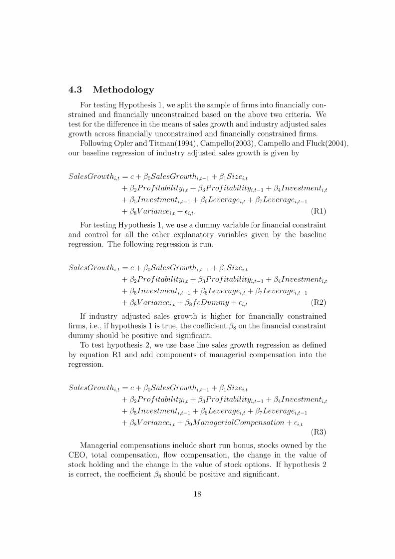
4.3 Methodology
For testing Hypothesis 1, we split the sample of firms into financially con-strained and financially unconstrained based on the above two criteria. Wetest for the difference in the means of sales growth and industry adjusted salesgrowth across financially unconstrained and financially constrained firms.
Following Opler and Titman(1994), Campello(2003), Campello and Fluck(2004),our baseline regression of industry adjusted sales growth is given by
SalesGrowthi,t = c+ β0SalesGrowthi,t−1 + β1Sizei,t
+ β2Profitabilityi,t + β3Profitabilityi,t−1 + β4Investmenti,t
+ β5Investmenti,t−1 + β6Leveragei,t + β7Leveragei,t−1
+ β8V ariancei,t + εi,t. (R1)
For testing Hypothesis 1, we use a dummy variable for financial constraintand control for all the other explanatory variables given by the baselineregression. The following regression is run.
SalesGrowthi,t = c+ β0SalesGrowthi,t−1 + β1Sizei,t
+ β2Profitabilityi,t + β3Profitabilityi,t−1 + β4Investmenti,t
+ β5Investmenti,t−1 + β6Leveragei,t + β7Leveragei,t−1
+ β8V ariancei,t + β8fcDummy + εi,t (R2)
If industry adjusted sales growth is higher for financially constrainedfirms, i.e., if hypothesis 1 is true, the coefficient β8 on the financial constraintdummy should be positive and significant.
To test hypothesis 2, we use base line sales growth regression as definedby equation R1 and add components of managerial compensation into theregression.
SalesGrowthi,t = c+ β0SalesGrowthi,t−1 + β1Sizei,t
+ β2Profitabilityi,t + β3Profitabilityi,t−1 + β4Investmenti,t
+ β5Investmenti,t−1 + β6Leveragei,t + β7Leveragei,t−1
+ β8V ariancei,t + β9ManagerialCompensation+ εi,t(R3)
Managerial compensations include short run bonus, stocks owned by theCEO, total compensation, flow compensation, the change in the value ofstock holding and the change in the value of stock options. If hypothesis 2is correct, the coefficient β8 should be positive and significant.
18
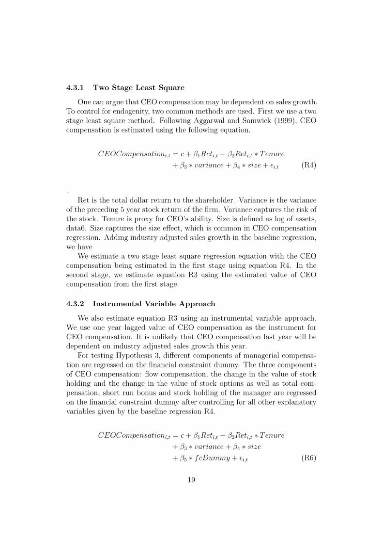
4.3.1 Two Stage Least Square
One can argue that CEO compensation may be dependent on sales growth.To control for endogenity, two common methods are used. First we use a twostage least square method. Following Aggarwal and Samwick (1999), CEOcompensation is estimated using the following equation.
CEOCompensationi,t = c+ β1Reti,t + β2Reti,t ∗ Tenure+ β3 ∗ variance+ β4 ∗ size+ εi,t (R4)
.Ret is the total dollar return to the shareholder. Variance is the variance
of the preceding 5 year stock return of the firm. Variance captures the risk ofthe stock. Tenure is proxy for CEO’s ability. Size is defined as log of assets,data6. Size captures the size effect, which is common in CEO compensationregression. Adding industry adjusted sales growth in the baseline regression,we have
We estimate a two stage least square regression equation with the CEOcompensation being estimated in the first stage using equation R4. In thesecond stage, we estimate equation R3 using the estimated value of CEOcompensation from the first stage.
4.3.2 Instrumental Variable Approach
We also estimate equation R3 using an instrumental variable approach.We use one year lagged value of CEO compensation as the instrument forCEO compensation. It is unlikely that CEO compensation last year will bedependent on industry adjusted sales growth this year.
For testing Hypothesis 3, different components of managerial compensa-tion are regressed on the financial constraint dummy. The three componentsof CEO compensation: flow compensation, the change in the value of stockholding and the change in the value of stock options as well as total com-pensation, short run bonus and stock holding of the manager are regressedon the financial constraint dummy after controlling for all other explanatoryvariables given by the baseline regression R4.
CEOCompensationi,t = c+ β1Reti,t + β2Reti,t ∗ Tenure+ β3 ∗ variance+ β4 ∗ size+ β5 ∗ fcDummy + εi,t (R6)
19

fcDummy is a dummy variable for financial constraint. If hypothesis 3is true, the coefficient on financial constraint dummy should be positive andsignificant.
The dataset is an unbalanced panel data of observations. The regressionsare estimated with both firm fixed effect and time effect. To control forheteroskedasticity, we report heteroskedastic adjusted standard errors. Tocontrol for auto correlation, our dependent variable is not in levels. Salesgrowth is used as a dependent variable instead of sales. Further, lag salesgrowth is included as an explanatory variable to control for any remainingautocorrelation.
5 Results
We test our first hypothesis by dividing the firms into financially con-strained and unconstrained firms. We estimate the standard t test to test ifthere is difference in the mean across the two groups of firms.
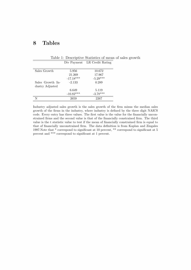
Table1
Table 1 reports the descriptive statistics mean sales growth and industryadjusted sales growth of the two groups of firms based on three criteria offinancial constraint. Industry adjusted sales growth is the sales growth ofthe firm minus the median sales growth of the firms in the industry, whereindustry is defined by the three digit NAICS code. Every entry has threevalues. The first value is the value for the financially unconstrained firmsand the second value is that of the financially constrained firm. The thirdvalue is the t statistic value to test if the mean of financially constrainedfirm is equal to that of financially unconstrained firm. For example, thefirst entry says that mean sales growth for financially unconstrained firmsis 5.956 and mean sales growth for financially constrained firms is 21.269where dividend payment is the financial constraint measure. The t statisticthat tests the difference between the mean sales growth of unconstrainedand constrained is -17.18 and it is significant at 1 percent significance level.We find that industry adjusted sales growth is higher for the financiallyconstrained firms supporting hypothesis 1 that the financially constrainedfirms are more aggressive in the output markets.
We test for hypothesis 1 by estimating the regression equation given byR2. The results are reported in table 2.
Table2
20

The coefficient on the dummy variable is positive and statistically sig-nificant for all the three criteria of financial constraint thereby providingempirical evidence in favor hypothesis 1.
We estimate the regression equation R3 by the two stage least squaremethod and report the results in table 3.
Table3
The first column of table 3 reports the baseline regression, given by equa-tion R1. In column 2, we report that short run bonus is positive and statisti-cally significant supporting hypothesis 2. In column 3, we document that thecoefficient of total compensation is positive and significant in support of hy-pothesis 2. We break up the total CEO compensation into three components,flow compensation, change in the value of stock holding and the change inthe value of stock options. Flow compensation coefficient is almost zero andstatistically insignificant. Change in the value of stock holding coefficient ispositive and statistically significant providing empirical evidence in favor ofhypothesis 2. But the coefficient of the change in the value of stock optionsis positive but statistically insignificant.
As a robustness measure, we estimate regression equation R3 employingthe instrumental variable approach. The resutls are documented in table 4.
Table4
The instrument for CEO compensation is lag values of CEO compensation.In column 3, the coefficient of total compensation is positive and significantsupporting hypothesis 2. We break up the total CEO compensation intothree components, flow compensation, change in the value of stock holdingand the change in the value of stock options. Flow compensation coefficientis almost zero and statistically insignificant. Change in the value of stockholding and the change in the value of stock options both have positive andstatistically significant coefficient.
Results from tables 3 and 4 suggest that the product market aggressive-ness is explained by CEO total compensation, SR bonus and Change in thevalue of stock holding even though the results for change in the value of stockoptions is mixed. We do not expect the coefficient of the flow compensationto be statistically significant as the flow compensation mainly consists offixed salary and long term payouts. The results from tables 3 and 4 are insupport of hypothesis 2.
We test for hypothesis 3 by estimating the regression equation R6 andreporting the results in tables 5 and 6. The dependent variable in this regres-sion estimation are the five compensation variables used in the estimation ofequation R3 and reported in tables 3 and 4.
21

Table5
Table6
The coefficient of financial constraint dummy is positive and significantusing both the measures of financial constraints providing empirical evidencefor hypothesis 3. The results suggest that the financially constrained firms’variable compensation are higher as compared to the firms which are finan-cially unconstrained.
6 Conclusion
We provide an additional factor which can explain the product marketdecisions of the firms. We document that the product market aggression de-pends on the variable component of the managerial compensation structure.Further, we report that the financially constrained firms are more aggressivein the product market. We also provide empirical evidence that the variablecompensation are higher for the financially constrained firms as comparedto the financially unconstrained firms. These results suggest that the ag-gressive product market behavior of the financially constrained firms may beexplained by the higher variable component of the managerial compensationof these firms.
22

7 Appendix
7.1 Appendix A1
Proof of Proposition 1
q∗1 =
z + θ + β1
(z)13 (3−λ2
3)− (1 + r)c− λ
3[z + θ + β2
(z)13 (3−λ2
3)− (1 + r + d)c]
(3− λ2
3)
(10a)and
q∗2 =
z + θ + β2
(z)13 (3−λ2
3)− (1 + r + d)c− λ
3[z + θ + β1
(z)13 (3−λ2
3)− (1 + r)c]
(3− λ2
3)
(10b)dq∗1dβ1
=1
z23 (3− λ2
3)2> 0
dq∗2dβ1
= −λ3
1
z23 (3− λ2
3)2
dq∗1dβ2
= −λ3
1
z23 (3− λ2
3)2
dq∗2dβ2
=1
z23 (3− λ2
3)2> 0
dq∗2dβ2− dq∗1dβ2
=1
z23 (3− λ2
3)2
(1 +λ
3) > 0
for all values of λ as long as assumption A1 holds (3− λ2
3) > 0
7.2 Appendix A2
dβ∗1dd
=λ3cz
13 (3− λ2
3)3
2√
3β∗ 12
2 D(14a)
dβ∗2dd
=
cz13 (3− λ2
3)[1− (3−λ
2
3)2z
23
2√3β
∗ 12
1
− λ2
9]
D(14b)
23

where
D = [1−(3− λ2
3)2z
23
2√
3β∗ 12
1
][1−(3− λ2
3)2z
23
2√
3β∗ 12
2
]− λ2
9
Using the FOC equation 10a and 10b, the maximized value of Vi can bewritten as
V ∗i =(β∗i )
32
332
.
Maximized net value of the firm is
V ∗i,net = V ∗i − wi
=(β∗i )
32
332
− (β∗i )2
2(z)23 (3− λ2
3)2− U.
U is the reservation utility which is positive. This implies that
(β∗i )32
332
>(β∗i )
2
2(z)23 (3− λ2
3)2
leading to(3− λ2
3)2z
23
2√
3β∗ 12
i
>3
4.
V ∗i,net is the maximized net value of firm i, maximized with respect to βi.Hence,
dV ∗i,netdβi
< 0
which leads to(3− λ2
3)2z
23
2√
3β∗ 12
i
< 1.
Hence we get the upper and lower limits
3
4<
(3− λ2
3)2z
23
2√
3β∗ 12
i
< 1,
−λ2
9< [1−
(3− λ2
3)2z
23
2√
3β∗ 12
2
− λ2
9] < 1− 3
4− λ2
9.
24

Sufficient condition for [1− (3−λ2
3)2z
23
2√3β
122
− λ2
9] < 0 is 3
2< λ.
−λ2
9< D = [1−
(3− λ2
3)2z
23
2√
3β121
][1−(3− λ2
3)2z
23
2√
3β122
]− λ2
9<
1
16− λ2
9
Sufficient condition for D to be negative is 34< λ.
If 32< λ , dβ2
dd> 0.2
So dβ2dd
> 0 when 32< λ . Further,when 3
2< λ, dβ1
dd< 0. So as long as
32< λ
dβ2dd− dβ1
dd> 0
Hence we show that as long as 32< λ,
dβ2dd
> 0
dβ2dd− dβ1
dd> 0.
We note that 32< λ is a sufficient condition for these to hold, not necessary
conditions. There can be other ranges of λ when these two inequalities mayhold.
7.3 Appendix A3
de2dd
=dβ2dd
de2dβ2
=1
z13 (3− λ2
3)
cz13 (3− λ2
3)[[1− (3−λ
2
3)12 z
23
2√3β
121
]− λ2
9]
D
=
c[[1− (3−λ2
3)12 z
23
2√3β
121
]− λ2
9]
D
2We only consider positive value of λ
25

de1dd
=dβ1dd
de1dβ1
=1
z13 (3− λ2
3)
λ3cz
13 (3− λ2
3)3z
23
2√
3β122 D
=λ3cz
23 (3− λ2
3)2
2√
3β122 D
where
D = [1−(3− λ2
3)2z
23
2√
3β121
][1−(3− λ2
3)2z
23
2√
3β122
]− λ2
9
dq2dd
=de2dd− c− λ
3de2dd
(3− λ2
3)
=c
(3− λ2
3)D
[(3− λ2
3)2z
23
2√
3β122
[[1−(3− λ2
3)12 z
23
2√
3β121
]− λ2
9]]
The sufficient condition for dq2dd
> 0 is that 32< λ. We should also note
that this is a sufficient condition for dq2dd> 0 but not a necessary condition.
Proceeding in the same way for q1, we get,
dq1dd
=de1dd
+ λ3c− λ
3de2dd
(3− λ2
3)
=cλ3
(3− λ2
3)D
(3− λ2
3)4z
43
12β121 β
122
The sufficient condition for dq1dd
< 0 is that 32< λ. We should also note
that this is a sufficient condition for dq1dd> 0 but not a necessary condition.
So when 32< λ,
dq2dd
> 0,
dq2dd
< 0,
dq2dd− dq1dd
> 0.
QED.
26

7.4 Appendix A4
The various data definitions are as follows :Sales is Data 12 from COMPUTSTAT. Sales Growth is defined as Sales
in year t minus Sales in year t-1 divided by Sales at year t-1. Proxy for firmaggressiveness is defined as Sales growth of a firm minus the mediansales growth of that industry. This is called industry adjustedsales growth. So if a firm is more aggressive in terms of sales than itspeers in the industry, this proxy variable should be positive. If the firm islagging behind others in the same industry, then this variable should comeas negative. Industry is defined as the NAICS code. NAICS code betterdescribes industry compared to SIC code. Profitability is defined as the sumof data18, Income before extraordinary items, and data14, Depreciation andAmmortization , divided by total assets, data6. All these data are fromCompustat database. Investment is defined as the ratio of data172 by data6,total assets. data 172 is net income (loss). Size is log of assets , log(data6).Leverage is defined as the ratio of data9, long term debt to total assets data6.
We get executive compensation data from ExecuComp. Short Run Bonusis defined as Bonus divided by total current compensation, TDC1 of Execu-Comp. Percentage of shares owned by executives is defined as shrown dividedby shrsout divided by 10. shrsout is the common shares outstanding. shrownis the shares owned by the executive. Following Aggarwal and Samwick (1999), CEO compensation is composed of three components : flow compen-sation, the change in the value of stock holding and the change in the valueof stock options. Flow compensation is easily calculated as TDC1, which isavailable from ExecuComp. TDC1 is composed of salary, bonus, total valueof stock options, long term incentive payouts, other annual compensationand all other, as is defined in ExecuComp manual. The change in the valueof stock holding is defined as the percentage of stocks held by the CEO atthe beginning of the fiscal year multiplied by shareholder dollar return. Totalreturn to shareholders are reported in ExecuComp in percentages. The dol-lar return is defined as the percentage total return multiplied by the marketvalue of the firm at the beginning of the fiscal year. Once we have the dollarreturn to shareholder, we can calculate the change in the value of stock hold-ing. The change in the value of stock options is a bit difficult to calculate. Wecalculate the value of old options as the sum of INMONEX and INMONUN.INMONEX is the value of the unexercised exercisable options. INMONUN isthe value of unexercised unexercisable options. The new options are definedas BLK-VALU, which the value of new options granted in ExecuComp. To-tal option value is the sum of old options and new options. Change in theoption value is the value of the option in year t minus the value of the option
27

in year t-1. The total value of CEO’s compensation package is defined as thesum of the flow compensation, the change in the value of stock holding andthe change in the value of stock options. The variance of preceding five yearsstock returns is termed as variance and is used a proxy for stock’s risk. Wecalculate CEO tenure using BECAMECEO from ExecuComp, which givesus the date an individual has become the CEO. CEO tenure acts a proxy forher abilities when we run pay performance sensitivity regressions.
28
8 Tables
Table 1: Descriptive Statistics of mean of sales growthDiv Payment LR Credit Rating
Sales Growth 5.956 10.67221.269 17.967
-17.18*** -5.29***Sales Growth In-dustry Adjusted
-2.133 0.289
6.649 5.119-10.82*** -3.78***
N 2659 2267
Industry adjusted sales growth is the sales growth of the firm minus the median salesgrowth of the firms in the industry, where industry is defined by the three digit NAICScode. Every entry has three values. The first value is the value for the financially uncon-strained firms and the second value is that of the financially constrained firm. The thirdvalue is the t statistic value to test if the mean of financially constrained firm is equal tothat of financially unconstrained firm. The data definition is from Kaplan and Zingales1997.Note that * correspond to significant at 10 percent, ** correspond to significant at 5percent and *** correspond to significant at 1 percent.

Table 2: Regression Results of Sales Growth on Financial Constraint.Div Payment KZ Index LR Credit rating
Lag Sales GrowthIndustry Adjusted
-0.049*** -0.078*** -0.055** -0.050***
0.018 0.022 0.024 0.017Size 0.000 0.000 0.000 0.000
0.001 0.001 0.001 0.001Profitability -0.309* -0.200 -0.097 -0.289
0.182 0.235 0.256 0.181Lag Profitability -0.919*** -0.974*** -0.1.046*** -0.903***
0.176 0.221 0.249 0.176Investment 0.909*** 0.839*** 0.857**** 0.898***
0.156 0.201 0.224 0.156Lag Investment 0.487*** 0.540*** 0.561*** 0.478***
0.153 0.192 0.223 0.153Leverage 0.114*** 0.079* 0.081 0.109***
0.036 0.047 0.055 0.037Lag Leverage -0.035 -0.021 -0.051 -0.036
0.036 0.044 0.049 0.036Cash Capital 0.000 0.006* 0.000 0.000
0.001 0.003 0.001 0.001Variance -4.655 -3.841 -5.848 5.903
10.222 10.539 58.129 10.218FC dummy 4.733* 7.000** 2.653*
3.793 3.218 1.563N 3180 2013 1868 3180R Square 0.385 0.472 0.457 0.386
Dependent variable is industry adjusted sales growth, which is (salest−salest−1)/salest−1
. The top value is the coefficient of the regression coefficient and the bottom one is thecorresponding standard error. The data definition is from Kaplan and Zingales 1997. Notethat * correspond to significant at 10 percent, ** correspond to significant at 5 percentand *** correspond to significant at 1 percent.
30

Table 3: Regression of Sales Growth on Managerial Compensation. 2 StageLeast Square Approach.
Lag Sales Growth In-dustry Adjusted
-0.038** -0.047** -0.063*** -0.039** -0.058*** -0.054***
0.018 0.017 0.019 0.018 0.018 0.018Size 0.000 0.000 0.0000 0.000 0.000 0.000
0.001 0.001 0.001 0.001 0.001 0.001
Profitability -0.312* -0.327* -0.263 -0.304* -0.333* -0.2360.180 0.179 0.189 0.180 0.183 0.187
Lag profitability -0.907*** -0.959*** -0.933*** -0.898*** -0.920*** -0.884***0.175 0.174 0.183 0.175 0.177 0.180
Investment 0.849*** 0.799*** 0.835*** 0.887*** 0.884*** 0.855***0.155 0.155 0.161 0.156 0.157 0.160
Lag Investment 0.522** 0.587*** 0.614*** 0.484*** 0.551*** 0.517***0.152 0.152 0.161 0.152 0.156 0.157
Leverage 0.121*** 0.109*** 0.128*** 0.125*** 0.118*** 0.127***0.036 0.036 0.038 0.036 0.037 0.038
Lag Leverage -0.059 -0.040 0.045 -0.057 -0.036 -0.0540.036 0.036 0.038 0.036 0.036 0.037
Cash Capital 0.000 0.000 0.000 0.000 0.000 -0.0010.001 0.001 0.001 0.001 0.001 0.001
Variance -1.671 -1.428 -5.135 -4.043 -3.955 -5.13510.136 10.125 10.183 10.149 10.107 10.262
SR Bonus 0.103***0.026
Tot comp 0.035***0.008
Flow comp 0.0050.007
Ch stock holding 0.058**0.028
Ch stock option 0.0440.011
N 3165 3180 2817 3165 3007 2983R Square 0.387 0.398 0.408 0.399 0.378 0.398
Dependent variable is industry adjusted sales growth, which is (salest−salest−1)/salest−1
. We include firm fixed effect and time effect. The top value is the coefficient of theregression coefficient and the bottom one is the corresponding standard error. The datadefinition is from Kaplan and Zingales 1997. Note that * correspond to significant at 10percent, ** correspond to significant at 5 percent and *** correspond to significant at 1percent.
31

Table 4: Regression of Sales Growth on Managerial Compensation. Instru-mental Variable approach.
L SalesGrowthIndus
-0.036** -0.032* -0.114*** -0.035** -0.087*** -0.103***
0.017 0.017 0.019 0.017 0.018 0.019Size -0.0004 0.001 0.002 0.001 0.002 0.003**
0.001 0.001 0.001 0.001 0.001 0.001
Profitability -0.190 -0.198 -0.131 -0.077 -0.171 -0.0820.168 0.167 0.179 0.165 0.170 0.180
Lag prof-itability
-0.605*** -0.627*** -0.656*** -0.547*** -0.711*** -0.373**
0.159 0.159 0.178 0.157 0.172 0.170
Investment 0.688*** 0.568*** 0.569*** 0.607*** 0.589*** 0.573***0.139 0.139 0.145 0.136 0.139 0.148
Lag invest-ment
0.209 0.306** 0.177 0.538**** 0.221
0.133 0.134 0.131 0.152 0.142Leverage 0.090*** 0.102*** 0.104*** 0.108*** 0.096** 0.110***
0.034 0.034 0.037 0.034 0.036 0.038Lag lever-age
-0.052 -0.079** -0.029 -0.058* -0.032 -0.052
0.034 0.034 0.037 0.034 0.035 0.037Variance -1.716 -1.823 -4.543 -5.232 -3.498 -4.377
11.567 10.554 10.779 10.665 10.611 10.145SR Bonus 0.295***
0.036Tot comp 0.060**
0.026Flow comp 0.004
0.007Ch of stockholding
0.078**
0.035Ch of stockoption
0.145**
0.066N 3524 3507 2694 3486 2957 2907
Dependent variable is industry adjusted sales growth, which is (salest−salest−1)/salest−1
. We include firm fixed effect and time effect. Instrument of a variable is the lag of thevariable. Every entry has two values. The top value is the coefficient of the regressioncoefficient and the bottom one is the corresponding standard error. The data definitionis from Kaplan and Zingales 1997. Note that * correspond to significant at 10 percent,** correspond to significant at 5 percent and *** correspond to significant at 1 percent.
32

Table 5: Regression of Managerial Compensation on Financial Constraint.Financial Constraint is based on Dividend Payment
Tot Comp Fl Comp Ch Stock Hold Ch Stock Opt SR Bonus
Ret 0.293*** 0.005 0.046*** 0.237*** 0.014*0.021 0.037 0.008 0.014 0.008
Ret*tenure -0.0001 -0.0002 -0.001*** 0.0011*** -0.00010.0002 0.0004 0.0000 0.0001 0.0001
Ret*var 2.456*** -0.043 1.0176*** 1.408*** 0.0500.168 0.209 0.065 0.117 0.065
Ret*size -0.00002*** -0.000 -0.0000*** -0.0000*** -0.0000*0.000000 0.000 0.0000 0.0000 0.0000
FCDummy
16.442* -0.994 -0.176 18.945*** 7.37**
9.247 14.025 3.102 6.466 3.110
N 1595 1775 1707 1665 1775
RSquare
0.735 0.158 0.3878 0.721 0.424
Sales Growth is (salest − salest−1)/salest−1. Sales growth in is industry adjusted salesgrowth. ret is dollar return to share holder which is defined as the total market value ofequity at the beginning of the year multiplied by the stock return including distributionsover the year. Variance is the preceding 60 months variance of the monthly return of thestock. Size is the log of assets. Tenure of the manager is calculated from Execucomp.Total compensation is divided into three components, flow compensation, change in valueof stock holding (ch of stock holding) and change in value of stock option (ch of stockoption).Short run bonus is defined as the ratio of bonus to flow compensation. Everyentry has two values. The top value is the coefficient of the regression coefficient and thebottom one is the corresponding standard error. Note that * correspond to significant at10 percent, ** correspond to significant at 5 percent and *** correspond to significant at1 percent.
33

Table 6: Regression of Managerial Compensation on Financial Constraint.Financial Constraint is based on Long Run Credit Rating of the firm
Tot Comp Fl Comp Ch Stock Hold Ch Stock Opt SR Bonus
Ret 0.366*** 0.007 0.059*** 0.296*** 0.022***0.027 0.036 0.008 0.018 0.007
Ret*tenure -0.0003 -0.0001 -0.001*** 0.0006*** -0.00000.0003 0.0004 0.0000 0.0002 0.0000
Ret*var 2.229*** 0.008 0.938*** 1.249*** -0.0470.233 0.311 0.0681 0.153 0.065
Ret*size -0.00003*** -0.000 -0.0000*** -0.0000*** -0.0000***0.000000 0.000 0.0000 0.0000 0.0000
FCDummy
18.134*** 4.76 0.955 11.820*** 5.046***
7.027 8.57 1.9717 4.426 1.788
N 1377 1533 1475 1437 1533
RSquare
0.564 0.123 0.360 0.604 0.379
Sales Growth is (salest − salest−1)/salest−1. Sales growth in is industry adjusted salesgrowth. ret is dollar return to share holder which is defined as the total market value ofequity at the beginning of the year multiplied by the stock return including distributionsover the year. Variance is the preceding 60 months variance of the monthly return of thestock. Size is the log of assets. Tenure of the manager is calculated from Execucomp.Total compensation is divided into three components, flow compensation, change in valueof stock holding (ch of stock holding) and change in value of stock option (ch of stockoption).Short run bonus is defined as the ratio of bonus to flow compensation. Everyentry has two values. The top value is the coefficient of the regression coefficient and thebottom one is the corresponding standard error. Note that * correspond to significant at10 percent, ** correspond to significant at 5 percent and *** correspond to significant at1 percent.
34

References
[1] Aggarwal R, Samwick A, 1999. The Other Side of theTrade-off:The Impact of Risk on Executive Compensation.Journal of Political Economy, 107, 65-105.
[2] Aggarwal R, Samwick A, 2003. Performance Incentiveswithin Firms: The Effect of Managerial Responsibility.Journal of Finance, 58, 1613-1649.
[3] Bolton P, 1990. Renotiation and Dynamics of ContractDesign. European Economic Review, 34, 303-310.
[4] Bolton P, Scharfstein DS, 1990. A Theory of Preda-tion Based on Agency Problems in Financial Contracting.American Economic Review, 80, 93-106.
[5] Bosshardt D, Patterson D, 1991. The Marginal Value ofManagement Using Stochastic Control. Journal of Eco-nomics Dynamics and Control, 15, 455-489.
[6] Brander J, Lewis T ,1986. Oligopoly and Financial Struc-ture: The Limited Liability Effect. American EconomicReview, 76, 956-970.
[7] Brander P,Lewis T, 1988. Bankrupcy Costs and the The-ory of Ologopoly. Canadian Journal of Economics, 21, 221-243.
[8] Campello M, 2003. Capital Structure and Product Mar-kets Interations: Evidence from Business Cycles. Journalof Financial Economics, 68, 353-378.
[9] Campello M, 2005. Debt Financing: Does it Boost or HurtFirm Performance in Product Markets. Journal of Finan-cial Economics, 82, 135-172.
[10] Campello M, Zsuzsanna Fluck, 2008. Product Market Per-formance, Switching Costs and Liquidation Values:TheReal Effects of Financial Leevrage. Working paper.
[11] Chen Ho-Chyuan, 2005. Strategic Debt and RJV Compe-tition. Australian Economic Papers, 46, 234-239.
35

[12] Chevalier JA, 1995a. Capital Structure and Product Mar-ket Competition:Empirical Evidence From the Supermar-ket Industry. American Economic Review, 85. 415-435.
[13] Chevalier JA, 1995b. Do LBO Supermarkets Charge More? An Empirical Analysis of the Effects of LBOs on Super-market Pricing. Journal of Finance, 50, 1095-1112.
[14] Chevalier JA, Scharstein DS, 1996. Capital Market Imper-fections and Counter Cyclical Markups:Theory and Evi-dence. American Economic Review, 86, 703-725.
[15] Diamond D, 1984. Financial Intermediation and DelegatedMonitoring. Review of Economic Studies, 51, 393-414.
[16] Faure-Grimaud A, 2000. Product Market Competition andOptimal Debt Contracts : the Limited Liability Effect Re-visited. European Economic Review, 44, 1823-1840.
[17] Fazzari S, Hubbard R, Peterson B, 1988. Financial Con-straints and Corporate Investments. Brooking Papers onEconomic Activity, 1, 141-191.
[18] Fudenberg D, Tirole Jean, 1986. A ‘Signal-Jamming’ The-ory of Predation. Rand Journal of Economics, 17, 366-376.
[19] Glazer J, 1994. The Strategic Effects of Long Term Debtin Imperfect Competition. Journal of Economic theory, 62,428-443.
[20] Gilchrist S, Himmelberg C, 1995. Evidence on the Roleof Cash Flow for Investment. Journal of Monetary Eco-nomics, 36, 541-572.
[21] Hendel I, 1996. Competition under Financial Distress.Journal of Industrial Economics, 44, 309-324.
[22] Jean-Baptiste Eslyn, Michael H Riordan, 2003. CapitalMarkets Contraint Industry scale. Columbia Universityworking paper.
[23] Malmendier U, Tate G, 2005. CEO Overconfidence andCorporate Investment. Journal of Finance, 60, 2661-2700.
36

[24] Michael Riordian, 2003. How do Capital Markets InfluenceProduct Market Competition ? Keynote Prsentation toInternational Industrial Organization Conference, Boston.April 4-5,2003.
[25] Khanna N, Tice S, 2000. Strategic Responses of In-cumbents to New Entry:The Effect of Ownership Struc-ture,Capital Structure. and Focus. Review of financialstudies, 13, 749-779.
[26] Kovenock D, Philips G , 1995. Capital Structure and Prod-uct Market Rivalry : How do We Reconcile Theory andEvidence ?. American Economic Review, 85, 403-408.
[27] Kovenock D, Phillips G, 1997. Capital Structure and Prod-uct Market Behavior:An Examination of Plant Exit andInvestment Decisions. Review of Financial Studies, 10,767-803.
[28] Maksimovic V , 1988. Capital Structure in RepeatedOligopolies. Rand Journal of Economics, 19, 389-407.
[29] Maskin E, Tirole, J. 1999. Unforseen Contingencies andIncomplete Contracts. Review of Economic Studies, 66,83-114.
[30] Maurer,B, 1999. Innovation and Investment under Finan-cial Constraints and Product Market Competition. Inter-national Journal of Industrial Organization, 17, 455-476.
[31] Opler TC, Titman S,1994. Financial Distress and Corpo-rate Performance. Journal of Finance, 49, 1015-1040.
[32] Philips GM, 1995. Increased Debt and Industry ProductMarkets:an Empirical Analysis. Journal of Financial Eco-nomics, 37, 189-238.
[33] Povel P , Raith M, 2003. Optimal Debt with UnobservableInvestments. Rand Journal of Economics, 35, 599-616.
[34] Povel P , Raith M, 2004. Finanical Constraints and Prod-uct Market Competition:Ex-ante vs Ex-post Incentives.International Journal of Industrial Organization, 22, 917-949.
37

[35] Raith M, 2003. Competition, Risk and Managerial Incen-tives. American Economic Review, 93, 1425-1436.
[36] Showalter D, 1995. Oligopoly and Financial Structure :Comment. American Economic Review, 85, 647-653.
[37] Showalter D, 1999. Strategic Debt: Evidence in Manufac-turing. International Journal of Industrial Organization,17, 319-333.
[38] Wang R, 2006. Executive Incentives and Financial Con-straints. Working Paper.
[39] Whited T, Wu G, 2003. Financial Constraints Risk. Work-ing Paper.
38