1

Excel Tutorial

Welcome to Excel!

This tutorial may look long and boring, but sit back, take a deep breath, and step through it. It will take one-two hours at most. After this tutorial you will use Excel in Biology 180 labs and class work often, and are expected to do so with relative ease.

Microsoft Excel is powerful and widely available spreadsheet software, used for tracking baseball statistics, stocks prices, business budgets, and of course, scientific data. Understanding how to store, manipulate, calculate, and analyze data in an Excel spreadsheet is a fundamental skill for Biology 180 and innumerable other pursuits.

Let’s get started!

Directions

You will need a computer with any recent version of Microsoft Excel installed to complete this take-home lab. Computers are available in the Biology Study Area (Hitchcock 220) or numerous other sites on campus. You also need to download the Excel_tutorial.xlsx data file from the Data section of the Bio 180 Home Page. You may work on this tutorial with other students either in person or by collaborating on the course GoPost. However, TAs will not answer questions about this tutorial.

Versions

Excel has been around a long time, first introduced for the Apple Macintosh in 1985, and then for the Windows PC in 1987. It is now part of the Microsoft Office Suite of software (a package that also includes Word, PowerPoint, Access, and other software). This tutorial covers very basic tasks and functions in Excel and will be applicable to every version every made, so we will only briefly cover some of the differences you

2

might encounter between versions before diving into the tutorial and exercises. The most common versions available today and version-specific guidance on how to use them are as follows:

Mac OSX Excel 2011 

While unfamiliar to some of you, Apple laptops are what we use in BIO 180 labs. Some Mac-specific tips for Excel 2011 include:

• Select the “Window” menu and “Zoom” once you open Excel to be sure the spreadsheet covers the screen properly

• Select “View” and “Normal” to leave the page layout view, a good way to simplify the layout for your work

• The laptops have “multi-touch” trackpads that allow for easy navigation of spreadsheets. Try it!

Windows Excel 2007 & 2010 

Along with the rest of the 2007 Microsoft Office Suite of software, Excel 2007 got a complete interface makeover, and continues in the 2010 version. The instructions in this manual may not match these newer menus and choices. Progress? It might come down to personal taste, but you should be able to hunt down the commands we use in this tutorial anyway.

• To easily share a document with users of earlier versions, choose the “File” menu and “Save As,” and select “97-2003 Document.”

In lab, you will use Excel 2011 on Macintosh laptops. While it’s okay to do this tutorial on a Windows computer, you will be better prepared for lab if you do it on a Mac.

3

All recent versions of Excel, on Windows or a Mac, can open the same data files (though you may need to download a free compatibility pack, for Mac or Windows, as mentioned above, if you try to open newer files with older software). Therefore you don’t have to worry too much about which kind of computer or Excel you have. Also note: if you are adventurous and/or poor, you can always try OpenOffice, a free and open-source office suite that is generally compatible with Microsoft Office files.

Formatting in this Tutorial

From now on, bold items in the text will correspond with menus or commands that you select with your mouse, and brackets and a [ different font ] will indicate something you should type into your spreadsheet like [ =AVERAGE(B12,B13) ], but ignoring the brackets. Keys will be shown in quotes, like the “Delete” and “Esc” keys. Steps in a series of instructions will be numbered, and separate guidance for Mac or Windows versions may be provided. If you are already familiar with Excel, review the =SUM(This) statements and skip topics you think you have already mastered – but beware, you could lose points on the quiz at the end if you aren’t careful.

The Basics

Getting Started

=SUM(This) Understand how to open Excel files and understand the basic Excel interface.

First, we’ll cover the real basics of launching Excel, what the important parts of its interface are, and how to save and open files.

1. Launch the Excel program on your computer.

Mac: Find the Excel icon on the icon dock and click it once. Be aware that the icon dock may be set to “hide” and will pop up only when you move the mouse to an edge the screen (the sides or bottom) and wait a second for it to pop up. If the Excel Workbook Gallery opens, select “Excel Workbook” and select Choose.

Windows: Open the Start Menu and select the Excel icon. It may be hidden in the All Programs button and then the Microsoft Office folder.

4

2. Observe the location of the following:

a. The Menu Bar is the row of words across the top of the program, often starting with "File, Edit, View...Data” etc. When told to select the Data menu, this is what you click. Yeah, I know - boring. Bear with us. Also note that keyboard shortcuts are listed next to menu commands, and you will find it faster to use them in most cases. Most keyboard shortcuts on a Windows computer start by holding down the “Ctrl” key, while on a Mac you press and hold “command ⌘” and then a second key. Many commands can be accessed through a pop-up menu by “right-clicking”, using a multi-button mouse, a multi-touch trackpad (Mac), or holding “control” when clicking (Mac).

b. The green ribbon has a series of tabs with “Home, Layout, Tables” etc. that allows quick access to many menu commands. The standard toolbar, located above the ribbon, also provides access to frequently used menu commands. Note: the locations of commands differ between Mac and Windows versions.

c. The formula bar, starting with an “ƒx” symbol, is where you can inspect and edit the contents of a cell in detail.

Mac: Sometimes the formula bar and ribbon are hidden, and need to be revealed by going to View and toggling on Formula Bar or Ribbon.

d. Notice the alphabetical column and numerical row labels. In combination, they describe individual cells, such as B15 or G34. You can resize the width of columns and height of rows by clicking on and dragging the line that separates their labels (feel free to try this).

e. Tabs for separate worksheets, similar to tabs used by newer web browsers, are shown at the bottom left, their default names being “Sheet1,Sheet2,” etc. They are all blank in a new document, and Excel documents may contain numerous worksheets. You can make new ones by clicking on the “+” tab or by selecting Insert, Worksheet. If there are many worksheets in a file, you may have to click on the right arrow (lower left corner of the sheet) to see the others.

3. Save and open files:

a. Since we are just getting started, you should be looking at a blank Excel file. Let’s save it with a new name.

i. Select File and Save. You should be able to name and save this Excel document. Name it whatever you like.

5

1. Always make note of where you are saving your documents so you don’t lose them. In the labs, the default is usually the desktop (the icon will appear right on the main screen, not in a hard drive or folder).

2. At any point that you want to start working on a new copy of a file, you may choose Save As instead. This stops overwriting the original file (if you have already saved it once or more), and lets you start a new file with contents identical to the original.

ii. Open the tutorial data file for further use in this tutorial, using File and Open, or by double-clicking its icon from Windows Explorer or the Mac Finder (Excel files, when opened this way, should automatically launch Excel to view and edit them). Now we are ready to get going!

Selecting, Moving, Copy & Paste

=SUM(This) Understand how to move or duplicate data around the spreadsheet.

These next few skills are some of the most essential and most often used for manipulating data in an Excel spreadsheet. Master them.

Before we do anything, remember that you can always use the Edit menu’s Undo command to correct mistakes. Continue to use this menu item (or the keyboard shortcut “ctrl-Z” (Windows) or “command ⌘-Z” (Mac)) as many times as needed until your data gets back to where it started. You can undo changes all the way back to when you started editing a document, in most cases.

1. Selecting cells, rows and columns

a. Click once on the cell that contains [Click Me!] in the middle of the tutorial spreadsheet you just opened. You will see a highlighted box around just that cell, indicating it has been selected

b. Now move the mouse pointer over the column heading labeled “D” at the top of the same column as that cell, and notice that the pointer changes to a downward-pointing arrow. Click once on the column header, and note that the entire column is selected.

c. Click and drag along several lettered column headings, and see that you can select several columns at once!

6

d. Do the same with the numbered row heading by clicking on the heading for row “8.” Voila!

e. Click once, anywhere else on the spreadsheet, to clear that highlighted multi-cell selection. Good job!

f. Now click and drag (holding the mouse down) from the [Click Me!] cell both to the right and down, and release the mouse button once you have selected [Select me too!]. Good, now keep that selected.

2. Moving things around

a. With all of those cells still selected, pass your mouse over the edge of the highlighted cells. Notice that the pointer changes to a hand.

b. Click and drag on the edge of the selected cells, and release the mouse button once you have moved the selected cells a few rows and/or columns. Notice that you are shown an indication of where the cells will “land” once you release the mouse button. If there is data already in the target cells, you will be alerted.

c. Now play with moving only a cell, a column, or a row, using the techniques shown above.

d. Look at the mess you’ve made! Use Edit, Undo to clean things up.

3. Copy and paste

Another way to move data around is by copying and pasting it. Instead of dragging the edges of selected cells, columns or rows, you can copy and paste them instead.

a. Select the two cells that contain the words [Four] and [Five], lower on the tutorial spreadsheet.

b. Select Edit and Copy from the menu bar, or use keyboard/mouse+ shortcuts. Notice that a moving dashed line now runs around the two cells you have selected to copy.

c. Click the empty cell where you want the top of the two cells to paste (just under the [three] in this case) and select Edit, Paste. Bravo! Note that choosing the Cut command would have also deleted the data from the original cells.

4. Non-adjacent cells

Sometimes the data you want to select isn’t in adjacent cells – so you can’t just drag a box around all the specific data you want to move or copy it. What to do?

7

Try this: Hold down the “Ctrl” key (Windows) or “command ⌘” (Mac), then click different cells all over the spreadsheet. You can even click-and-drag areas of cells in different parts of the spreadsheet. See how you highlight whatever you click or select while that key is held down?

Insert, Delete and Clear

=SUM(This) Understand how to insert rows and columns, and the difference between clear and delete.

Sometimes you need room for new data between columns of existing data. Other times you want to delete entire rows of data, or clear the contents of an area of the spreadsheet without changing how your data is layout. The insert, delete and clear commands are your answer.

1. Insert Columns or Rows

a. To insert a new column, highlight a cell in the column to the immediate right of where you need a new column. Select Insert, Column and a new one will be inserted. Do this anywhere you like, and notice that everything shifts one column to the right.

b. You can Insert a Row in a similar way.

2. Delete rows or columns

“Delete” and “Clear” are similar, but Delete will remove an entire row or column, but Clear will just remove the data in a cell, but leave rows and columns intact.

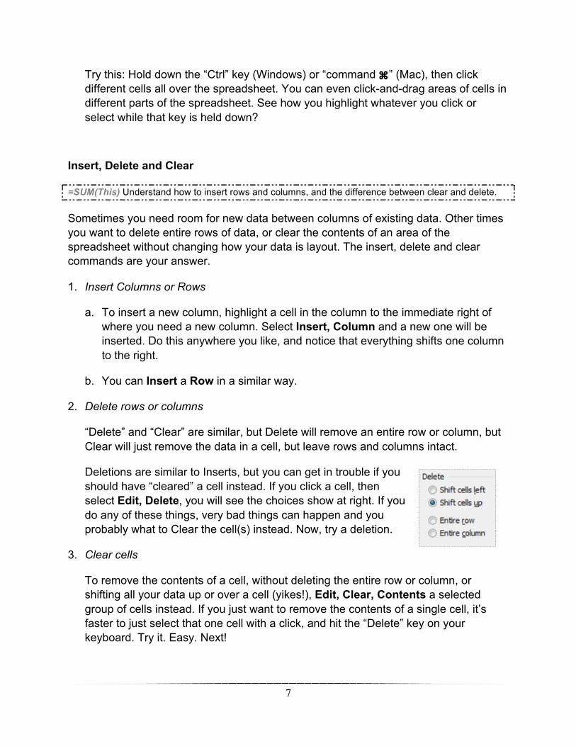
Deletions are similar to Inserts, but you can get in trouble if you should have “cleared” a cell instead. If you click a cell, then select Edit, Delete, you will see the choices show at right. If you do any of these things, very bad things can happen and you probably what to Clear the cell(s) instead. Now, try a deletion.

3. Clear cells

To remove the contents of a cell, without deleting the entire row or column, or shifting all your data up or over a cell (yikes!), Edit, Clear, Contents a selected group of cells instead. If you just want to remove the contents of a single cell, it’s faster to just select that one cell with a click, and hit the “Delete” key on your keyboard. Try it. Easy. Next!

8

Editing, Sorting, and Filtering Data

Let’s move on to changing and manipulating data. By now you may have figured out that you can click in a cell and edit or enter new data, but we have provided you with some sample data to speed things up. Select the “Editing & Sorting” worksheet tab at the bottom of the Excel_Tutorial data file, and let’s edit and sort the heck out of it.

The Database Format of Excel Spreadsheets

=SUM(This) Understand the usual organization of Excel spreadsheet data.

The first thing you should notice is that most Excel data is organized like a simple database, with a new database record represented by each row. More simply put, each row of data down the page represents a different individual, transaction, observation, object, etc. Each column, on the other hand, defines the kind of data collected for that unique individual, observation, etc. Even more simply: Rows are “unique things” and columns are “data kinds.” Where a row and column intersect, that cell contains the data for the corresponding “kind,” as recorded for that “thing.” There’s no reason this row and column convention couldn’t be flipped, but let’s stick to this format because it is the most common and Excel uses this as its default. Example:

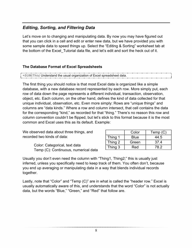
We observed data about three things, and recorded two kinds of data:

Color: Categorical, text data Temp (C): Continuous, numerical data

Usually you don’t even need the column with “Thing1, Thing2;” this is usually just inferred, unless you specifically need to keep track of them. You often don’t, because you end up averaging or manipulating data in a way that blends individual records together.

Lastly, note that “Color” and “Temp (C)” are in what is called the “header row.” Excel is usually automatically aware of this, and understands that the word “Color” is not actually data, but the words “Blue,” “Green,” and “Red” that follow are.

Color Temp (C) Thing 1 Blue 44.5 Thing 2 Green 37.4 Thing 3 Red 78.2

9

Formatting Data

=SUM(This) How to inspect and change the formatting of cells of data.

Let’s look closer at the data in our table’s cells (we are on the Editing & Sorting worksheet now). This data records the features of a few recent Bio 180 students. Look at all the columns of data in the tutorial spreadsheet, and follow along:

1. Defining Data Formats

a. Let’s start with the first column of data, “Height”. Select the entire column (Click the “A” at the top).

b. Select Format, Cells. You may do this a lot, so make a note of the keyboard shortcut, Ctrl or command ⌘- 1 (the number “1” key).

c. Right now the format of this data is undefined, and defaults to “General.” Let’s tell Excel that this data is numerical, and select “Number” from the list of categories.

d. Great. This now lets us do things like set the number of decimal points we want displayed. Just for fun, choose 0, and select “Okay” to leave this window. You should notice a change in how that column’s data is displayed. Also note that Excel understood that the word “Height” was the header row for the column, and didn’t try to format it as numerical data.

2. Incorrect Data Formats

Now let’s do this again, but wrong. That’s right: dare to be bad. Select Format, Cells again, with the first column of data selected. This time, change the format to “Time” and hit “Okay.” Yikes! This is an example of what can happen if you choose the wrong format. Usually it is obvious, but not always. Edit, Undo this change.

Sorting Data

=SUM(This) How to sort data without damaging relationships between columns or rows.

Sorting is one of the most important things you can do with your data, but it is also dangerous. For example, if you only sort the data in one column, but not adjacent

10

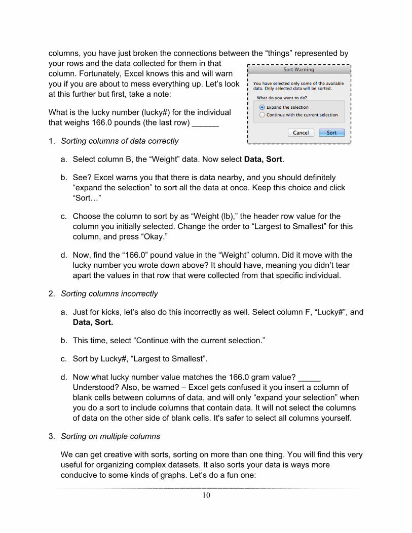
columns, you have just broken the connections between the “things” represented by your rows and the data collected for them in that column. Fortunately, Excel knows this and will warn you if you are about to mess everything up. Let’s look at this further but first, take a note:

What is the lucky number (lucky#) for the individual that weighs 166.0 pounds (the last row) ______

1. Sorting columns of data correctly

a. Select column B, the “Weight” data. Now select Data, Sort.

b. See? Excel warns you that there is data nearby, and you should definitely “expand the selection” to sort all the data at once. Keep this choice and click “Sort…”

c. Choose the column to sort by as “Weight (lb),” the header row value for the column you initially selected. Change the order to “Largest to Smallest” for this column, and press “Okay.”

d. Now, find the “166.0” pound value in the “Weight” column. Did it move with the lucky number you wrote down above? It should have, meaning you didn’t tear apart the values in that row that were collected from that specific individual.

2. Sorting columns incorrectly

a. Just for kicks, let’s also do this incorrectly as well. Select column F, “Lucky#”, and Data, Sort.

b. This time, select “Continue with the current selection.”

c. Sort by Lucky#, “Largest to Smallest”.

d. Now what lucky number value matches the 166.0 gram value? _____ Understood? Also, be warned – Excel gets confused it you insert a column of blank cells between columns of data, and will only “expand your selection” when you do a sort to include columns that contain data. It will not select the columns of data on the other side of blank cells. It's safer to select all columns yourself.

3. Sorting on multiple columns

We can get creative with sorts, sorting on more than one thing. You will find this very useful for organizing complex datasets. It also sorts your data is ways more conducive to some kinds of graphs. Let’s do a fun one:

11

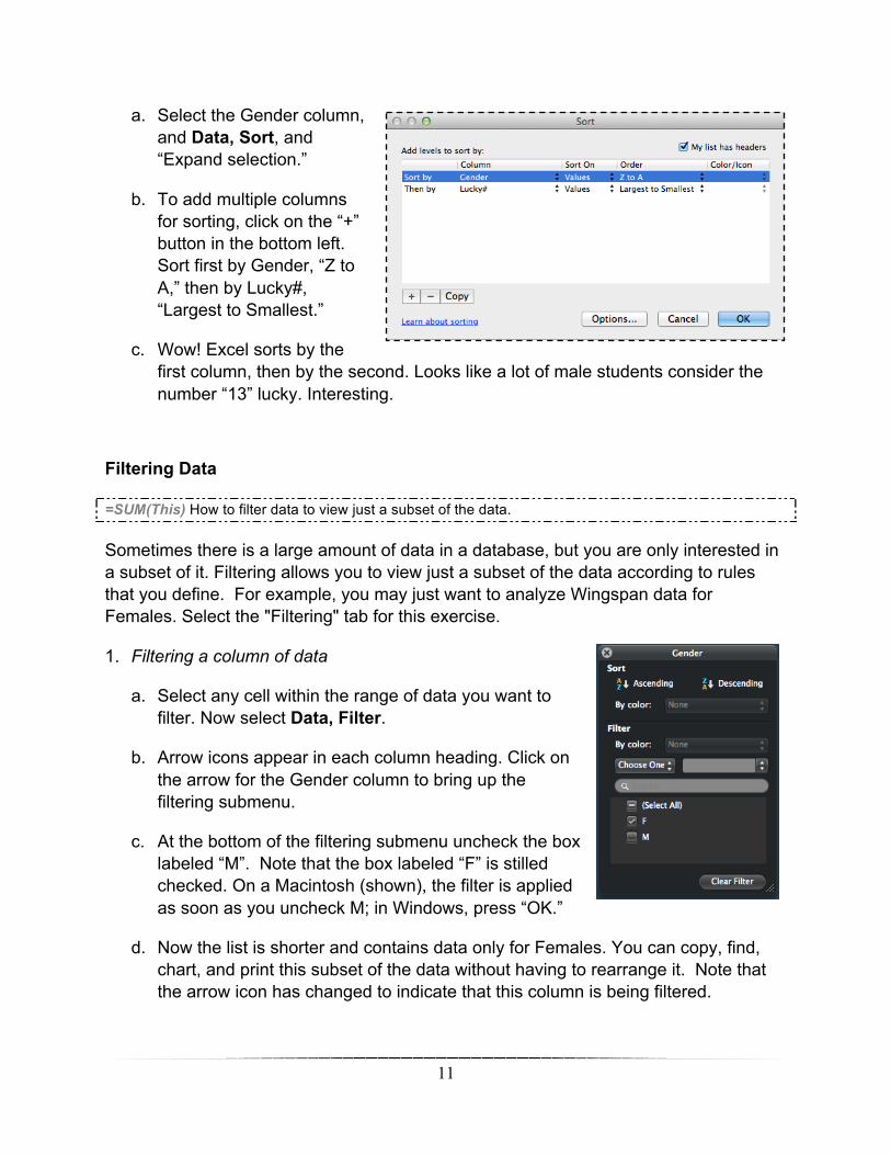
a. Select the Gender column, and Data, Sort, and “Expand selection.”

b. To add multiple columns for sorting, click on the “+” button in the bottom left. Sort first by Gender, “Z to A,” then by Lucky#, “Largest to Smallest.”

c. Wow! Excel sorts by the first column, then by the second. Looks like a lot of male students consider the number “13” lucky. Interesting.

Filtering Data

=SUM(This) How to filter data to view just a subset of the data.

Sometimes there is a large amount of data in a database, but you are only interested in a subset of it. Filtering allows you to view just a subset of the data according to rules that you define. For example, you may just want to analyze Wingspan data for Females. Select the "Filtering" tab for this exercise.

1. Filtering a column of data

a. Select any cell within the range of data you want to filter. Now select Data, Filter.

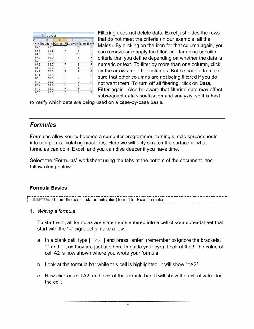
b. Arrow icons appear in each column heading. Click on the arrow for the Gender column to bring up the filtering submenu.

c. At the bottom of the filtering submenu uncheck the box labeled “M”. Note that the box labeled “F” is stilled checked. On a Macintosh (shown), the filter is applied as soon as you uncheck M; in Windows, press “OK.”

d. Now the list is shorter and contains data only for Females. You can copy, find, chart, and print this subset of the data without having to rearrange it. Note that the arrow icon has changed to indicate that this column is being filtered.

12

Filtering does not delete data. Excel just hides the rows that do not meet the criteria (in our example, all the Males). By clicking on the icon for that column again, you can remove or reapply the filter, or filter using specific criteria that you define depending on whether the data is numeric or text. To filter by more than one column, click on the arrows for other columns. But be careful to make sure that other columns are not being filtered if you do not want them. To turn off all filtering, click on Data, Filter again. Also be aware that filtering data may affect subsequent data visualization and analysis, so it is best

to verify which data are being used on a case-by-case basis.

Formulas

Formulas allow you to become a computer programmer, turning simple spreadsheets into complex calculating machines. Here we will only scratch the surface of what formulas can do in Excel, and you can dive deeper if you have time.

Select the “Formulas” worksheet using the tabs at the bottom of the document, and follow along below:

Formula Basics

=SUM(This) Learn the basic =statement(value) format for Excel formulas.

1. Writing a formula

To start with, all formulas are statements entered into a cell of your spreadsheet that start with the “=” sign. Let’s make a few:

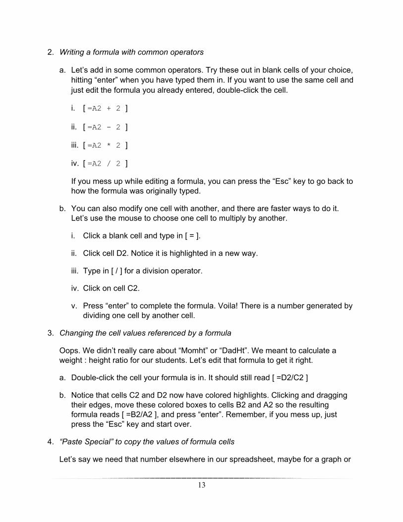
a. In a blank cell, type [ =A2 ] and press “enter” (remember to ignore the brackets, “[“ and “]”, as they are just use here to guide your eye). Look at that! The value of cell A2 is now shown where you wrote your formula

b. Look at the formula bar while this cell is highlighted. It will show “=A2”

c. Now click on cell A2, and look at the formula bar. It will show the actual value for the cell.

13

2. Writing a formula with common operators

a. Let’s add in some common operators. Try these out in blank cells of your choice, hitting “enter” when you have typed them in. If you want to use the same cell and just edit the formula you already entered, double-click the cell.

i. [ =A2 + 2 ]

ii. [ =A2 - 2 ]

iii. [ =A2 * 2 ]

iv. [ =A2 / 2 ]

If you mess up while editing a formula, you can press the “Esc” key to go back to how the formula was originally typed.

b. You can also modify one cell with another, and there are faster ways to do it. Let’s use the mouse to choose one cell to multiply by another.

i. Click a blank cell and type in [ = ].

ii. Click cell D2. Notice it is highlighted in a new way.

iii. Type in [ / ] for a division operator.

iv. Click on cell C2.

v. Press “enter” to complete the formula. Voila! There is a number generated by dividing one cell by another cell.

3. Changing the cell values referenced by a formula

Oops. We didn’t really care about “Momht” or “DadHt”. We meant to calculate a weight : height ratio for our students. Let’s edit that formula to get it right.

a. Double-click the cell your formula is in. It should still read [ =D2/C2 ]

b. Notice that cells C2 and D2 now have colored highlights. Clicking and dragging their edges, move these colored boxes to cells B2 and A2 so the resulting formula reads [ =B2/A2 ], and press “enter”. Remember, if you mess up, just press the “Esc” key and start over.

4. “Paste Special” to copy the values of formula cells

Let’s say we need that number elsewhere in our spreadsheet, maybe for a graph or

14

table to print out, and we want to copy it. There’s a trick involved.

a. Click your formula cell, the one that is now [ =B2/A2 ], and Edit, Copy it.

b. Click another empty cell and Edit, Paste. Did the same number show up in the pasted cell? No! Why not! Because you copied and pasted a formula, not the number value it calculated. Click this new cell and look at the formula bar, or double-click this new cell to see for sure. So, what do we do?

c. Simple. Go back and Edit, Copy the first formula cell again.

d. Then click and highlight the cell you just want to paste the numerical value, but not the formula.

e. Select Edit, Paste Special and then choose “Values” from all the choices you are given. Done! You now have a cell that is just the value, and is not tied to any source data or formula.

The big lesson: Any time you have strange copy-and-paste behavior in your spreadsheet, it’s probably because you are copying formulas and not plain-old numbers. However, sometimes you really do want to copy a formula, and we’ll look at that next.

5. Copying formulas and relative cell references

Now we will do something you should really know how to do (things are getting more and more important in this tutorial, if you hadn’t noticed). Sometimes you do want to copy and paste formulas so they apply to a whole column or row of data:

a. First, let’s make some room. Select all of column C, and the Insert, Columns.

b. Let’s give this column a new header row value, and call it “Hgt-Wt Ratio” or something similar

c. Let calculate the first one, in cell C2, with [ =A2/B2 ], enter.

d. Now the fun part – select and Edit, Copy that cell with the formula.

e. Click and drag to select all the empty cells in this column down to the end of the rows of data.

f. Edit, Paste that one original formula cell into all these empty ones. Wow!

In this case, we did want the formula, and not just that first calculated value, to paste into all those cells. It worked wonderfully, but we aren’t done.

15

g. Just for fun, let’s show all these calculated values with four decimal points. Select all of them, and then Format, Cells. Set these cells and numerical, and change the decimal points to four.

6. Functions in formulas

So far we’ve only used common operators (+ - * /) in formulas, but there are also many functions that Excel understands, to calculate sums, averages, square roots, and much more. Let’s use a common one for practice:

a. Click and select that empty cell at the bottom of your height : weight column you just made. It should be C26.

b. First, this is going to be a formula, so type in [ = ] to start.

c. Continue until you have typed [ =AVERAGE( ]. As you are typing Excel will suggest different functions and you may select the AVERAGE function. When you type that first open parenthesis (or after selecting the function), you’ll be prompted with a reminder of the formatting the AVERAGE function wants, which is a list of cells or values to use when calculating a mean for them.

d. You can now click-and-drag to select all the cells of ratios in this column. As you do, you’ll see the formula changing until it looks like [ =AVERAGE(C2:C25 ]. Good.

e. Now type the final “)” to complete this formula as [ =AVERAGE(C2:C25) ] and press “enter”.

f. There it is, the mean height ; weight ratio for all your data! Just to make it feel better, let’s select it and press the keyboard shortcut to make the contents of this cell bold, with a “Ctrl” or “command ⌘ - B”.

To explore what other functions are available, you can click the “ƒx” symbol on the Function Bar, search for them by name or browse long lists of them.

g. One last thing, just to reinforce your understanding of formulas: Edit, Copy and Edit, Paste this averaging formula cell to the empty cell just to its right, in column D. Presto! It’s the average for all the “MomHt” data.

h. Double-click this new cell to just confirm that the formula is now referring to a newly highlighted area including all the values in the column above it.

16

Charts / Graphs

Once you have collected and organized data, it is almost always useful to graphically represent it. Excel gives you a lot of options when making charts (or “graphs;” these words usually are synonymous but “chart” is used in Excel). We will not get into the details in this tutorial, but be aware of this super-easy way to make a chart:

Basic Charts

=SUM(This) How to select relevant data and create a graph.

1. Inserting a Chart

a. Select two columns of data, including the descriptive header row. Choose any ones you like.

b. Select the Chart tab on the Ribbon and choose Scatter under Insert Chart. Pick the Marked Scatter option. Voila! The chart is now displayed on the worksheet.

c. You can further refine the graph using the options under the green Chart tab and the two purple tabs Chart Layout and Format in the ribbon, which are available to you later whenever you select the your chart.

d. That’s it! You can now move your chart on your worksheet, and the data should be labeled using the header row descriptions in the data.

Quiz

Now you are ready to test your knowledge of Excel with an online quiz.

The online quiz is found under the “Lab – Excel Tutorial Quiz” link on the Bio 180 Home Page. You will need to use the last “Quiz Data” worksheet in the Excel_tutorial.xlsx file to complete the quiz, so don’t throw that file out just yet!