Excel Spreadsheets for the Classroom Teacher

• A workshop designed for teachers, by teachers

Overview

• Excel is a spreadsheet program that is used for a variety of purposes such as making worksheets, performing calculations, and creating graphs.

• Can you think of a personal way you could use Excel?

Getting Acquainted

One of the main features of Excel is that it consists of a series of columns and rows. Columns are labeled by letters (A-IV) and rows by numbers (1-65,536.) The intersection of a row and column is called a “cell”.

When you type information in a cell, it appears both in the cell and beneath the toolbars in what is called the “formula bar”.

When you finish typing in a cell, press “Enter” to have the computer accept the data.

Vocabulary

• Cells: the rectangles formed by the intersection of a row and column

• Active Cell: The cell with the black border around it that you are currently using

• Formula Bar: The long white bar under the toolbar that keeps

track of what you are typing

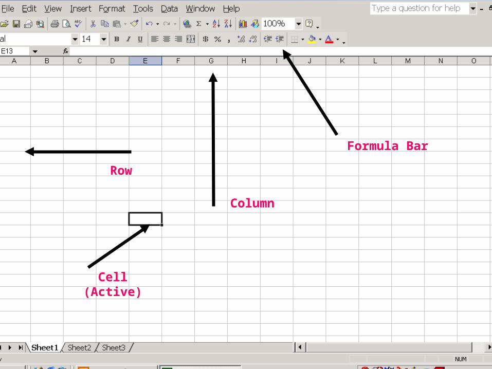
Column

Row

Cell (Active)

Formula Bar

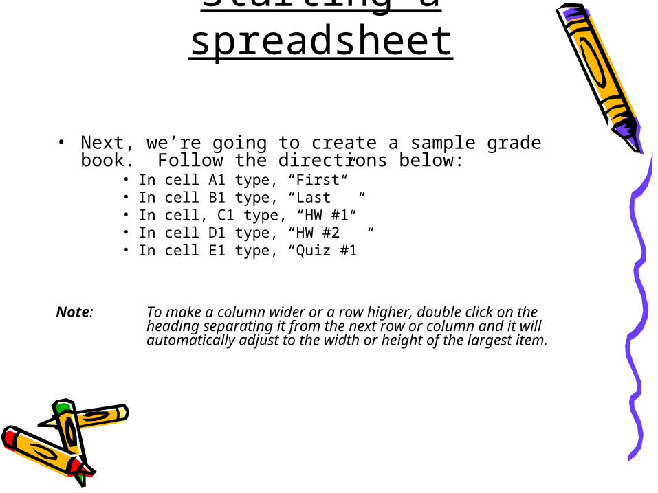
Starting a spreadsheet

• Next, we’re going to create a sample grade book. Follow the directions below:

• In cell A1 type, “First”• In cell B1 type, “Last”• In cell, C1 type, “HW #1”• In cell D1 type, “HW #2”• In cell E1 type, “Quiz #1”

Note: To make a column wider or a row higher, double click on the heading separating it from the next row or column and it will automatically adjust to the width or height of the largest

item.

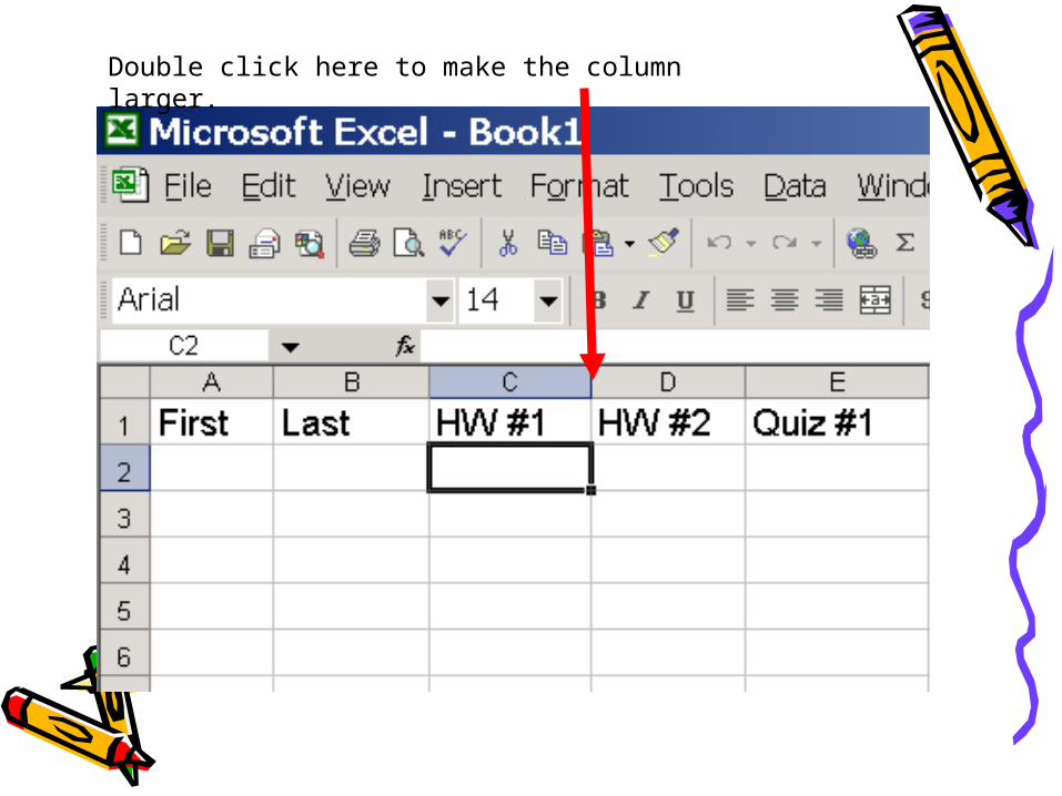
Double click here to make the column larger.

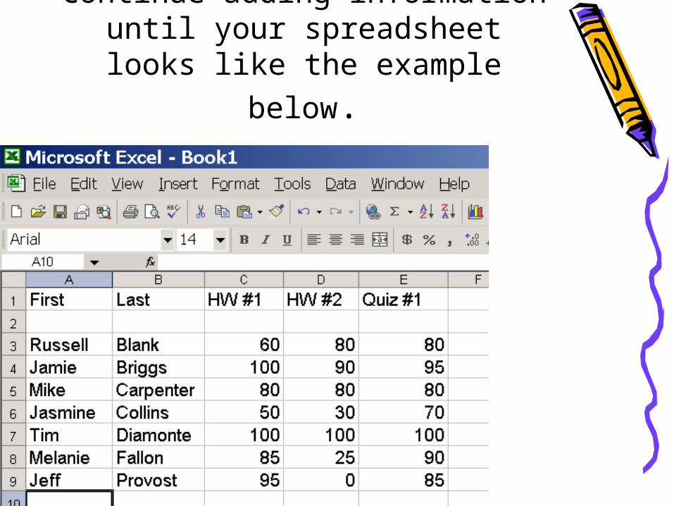
Continue adding information until your spreadsheet looks like

the example below.

• To jazz up the look of your spreadsheet you can apply a variety of format changes such as borders, shading, color changes, font changes, font size, etc. To make a change, select the cells you want to alter and then click on the desired effect from the formatting toolbar.

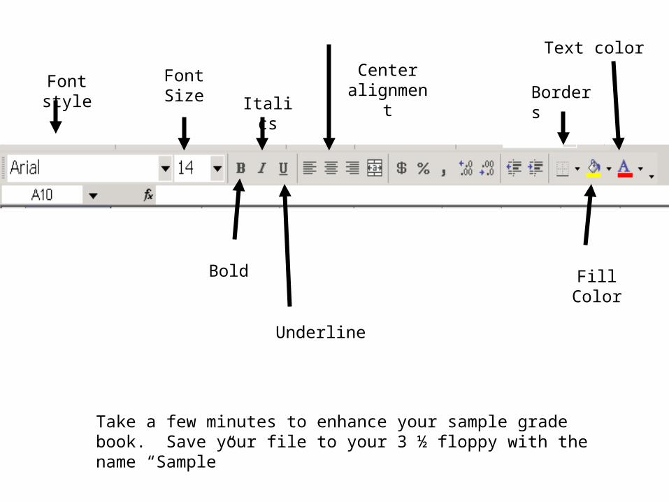
Font style Font Size

Bold

Underline

Italics

Center alignmen

tBorders

Text color

Fill Color

Take a few minutes to enhance your sample grade book. Save your file to your 3 ½ floppy with the name “Sample”

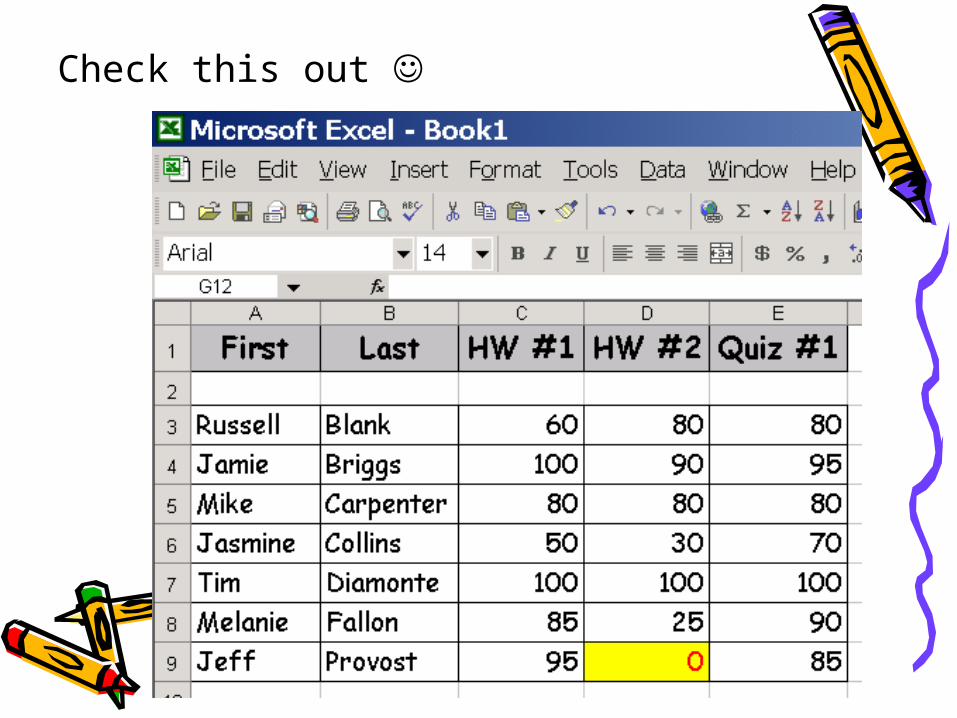
Check this out

Using AutoSum

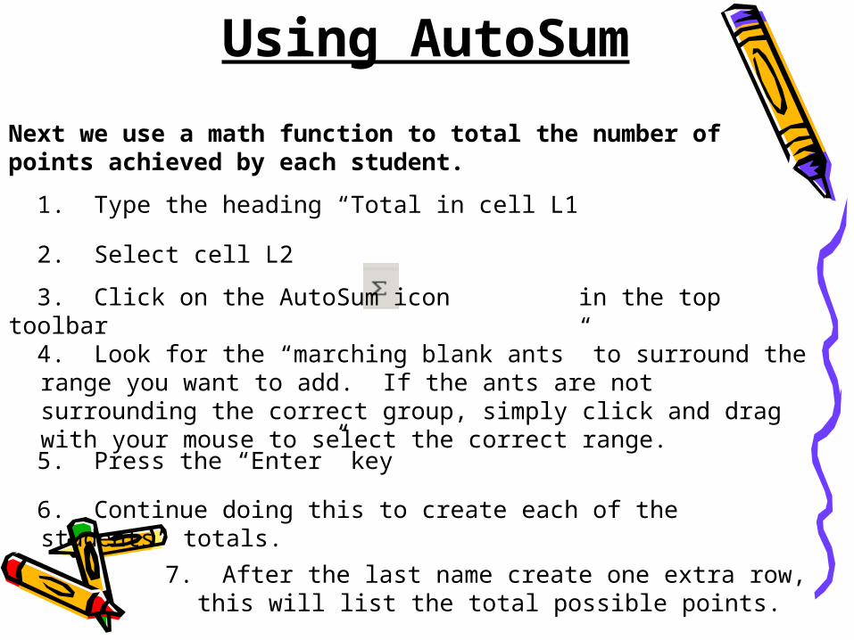
Next we use a math function to total the number of points achieved by each student.

1. Type the heading “Total in cell L1

2. Select cell L2

3. Click on the AutoSum icon in the top toolbar

4. Look for the “marching blank ants” to surround the range you want to add. If the ants are not surrounding the correct group, simply click and drag with your mouse to select the correct range.

5. Press the “Enter” key

6. Continue doing this to create each of the students’ totals.

7. After the last name create one extra row, this will list the total possible points.

Formulas

7. Continue this through the last name on your list, again the first cell will change L3/L26…

This step will allow you to create the student’s average for the quarter.

1. Enter the title “Average” in cell M1

2. Click on cell M2.

3. Click on the = sign on the menu board.

4. Select “Average”.

5. After Average type in “L2/by the cell below your last student which would be the total number of points. I.e.. L2/L26.

6. Click on “ok”

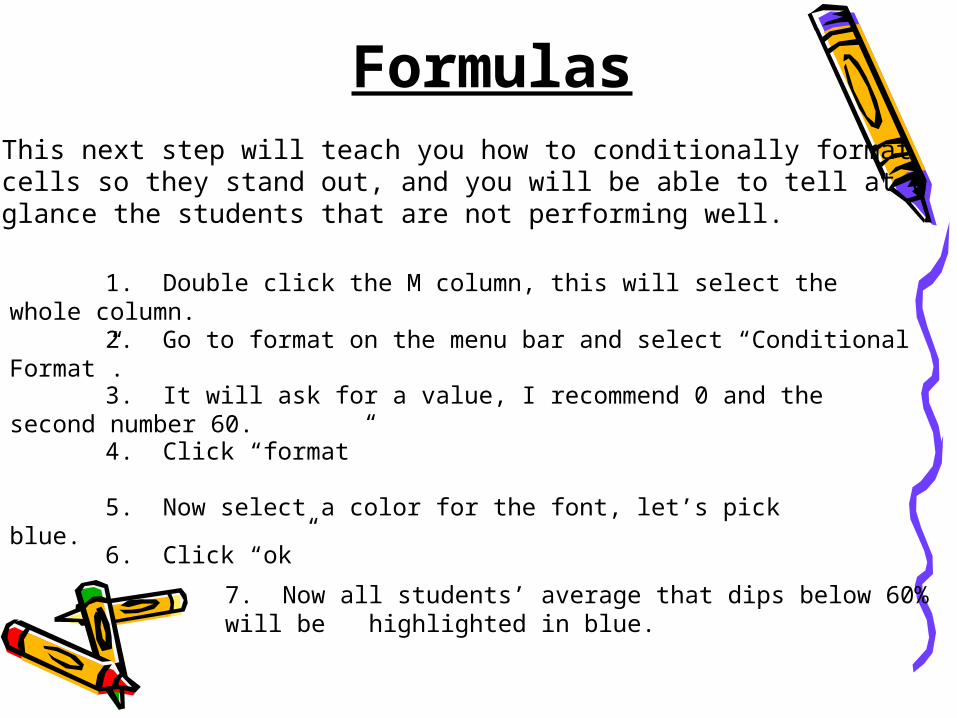
FormulasThis next step will teach you how to conditionally format cells so they stand out, and you will be able to tell at a glance the students that are not performing well.

1. Double click the M column, this will select the whole column.

2. Go to format on the menu bar and select “Conditional Format”.

3. It will ask for a value, I recommend 0 and the second number 60.

4. Click “format”

5. Now select a color for the font, let’s pick blue.

6. Click “ok”

7. Now all students’ average that dips below 60% will be highlighted in blue.

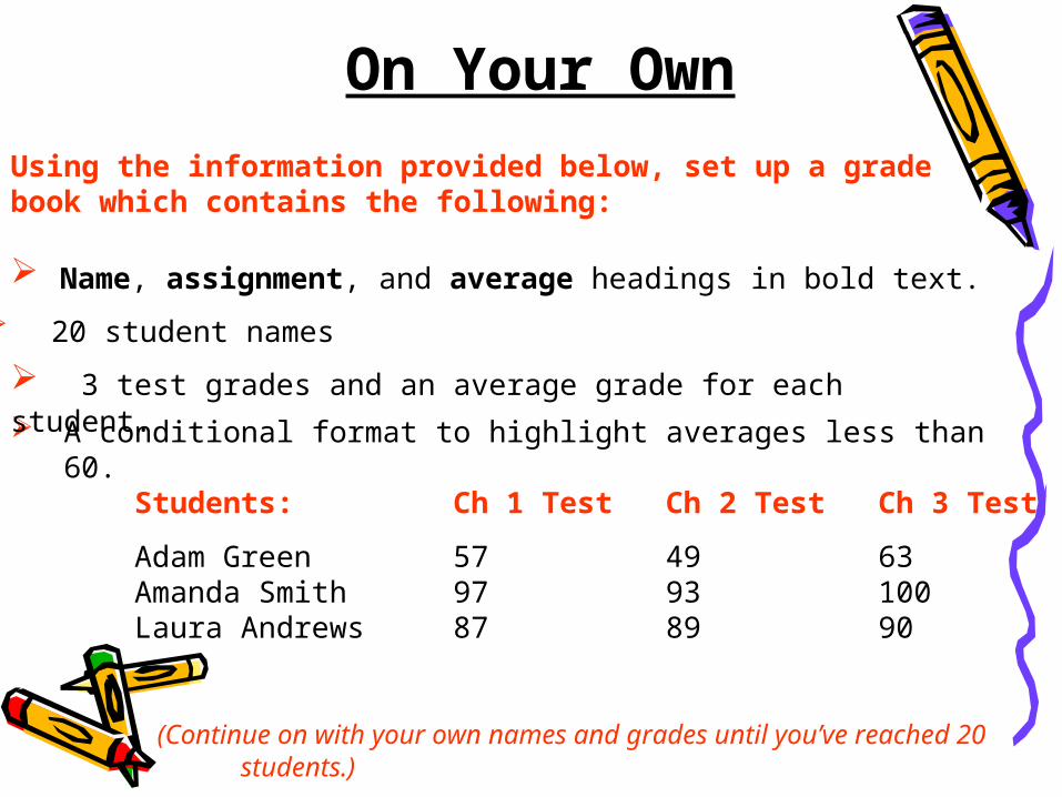
On Your Own

A conditional format to highlight averages less than 60.

Students: Ch 1 Test Ch 2 Test Ch 3 Test

Adam Green 57 49 63Amanda Smith 97 93 100Laura Andrews 87 89 90

(Continue on with your own names and grades until you’ve reached 20 students.)

Using the information provided below, set up a grade book which contains the following:

Name, assignment, and average headings in bold text.

20 student names

3 test grades and an average grade for each student.

The Final Product

Your final grade book should look something like this: