MICROSOFT EXCEL II

2003

University of South Florida Health Sciences Center Information Services

Education/Training Programs

2

Table of Contents

OBJECTIVE 4

THE OBJECTIVE OF THIS DOCUMENT IS TO PREPARE THE USER. THIS IS THE SECOND DOCUMENT IN A FOUR-PART SERIES. IT IS USED AS A GUIDE TO HELP ONE NAVIGATE THROUGH THE APPLICATION, AND IT IS DESIGNED TO COMPLEMENT THE CLASS TAUGHT HERE AT THE UNIVERSITY OF SOUTH FLORIDA'S HEALTH SCIENCES CENTER. 4

HOW TO… ERROR! BOOKMARK NOT DEFINED. Freeze Rows and Columns 5 Conditional Formatting 5

ADVANCED FORMULAS 6 Relative and Absolute Cell References 6 $Absolute $Cells 6

IF FUNCTIONS 6 Over Budget or Within Budget Formula 6 Grading Scale Formula 7 Lookup Function 8 Plus and Minus Grading Scale 9

DATE AND TIME FUNCTIONS 10 Date Function 10

DATABASE FUNCTIONS 11 DCOUNT function 11 DMAX Function 12 DMIN Function 14 DSUM Function 14

EXCEL TEMPLATES 15 Templates on my computer 15 Templates on Microsoft Office Online 17

WORKSHEETS AND WORKBOOKS 17 Open Two Worksheets at Once 17 Working with Multiple Worksheets 18

REVIEWING A DOCUMENT 19 Reviewing Toolbar Buttons 19 To Get the Reviewing Toolbar on Your Screen for Microsoft Word: 19

3

The functions that you will see on the Reviewing Toolbar are: 19

USING COMMENTS: 19 To insert a comment 19 Editing a Comment 20 Previous Comment 20 Next Comment 20 Delete the Comment 20 Tracking Changes 20 Turn on change tracking for a workbook 21 View tracked changes 21 Select the changes you want to see: 21 Changes made after a particular date 21 Changes made by a specific user 22

SELECT HOW YOU WANT TO VIEW THE CHANGES 22 Highlight the worksheet 22 Listed on a separate sheet 22 Going to the Previous Change 22 Going to the Next Change 22 Accept and reject changes 22

SELECT THE CHANGES TO REVIEW 22 Changes made after a particular date 23 Changes made by another user 23 Changes made by all users Error! Bookmark not defined. Changes to a specific area 23 Changes to the entire workbook 23

SENDING A REVISED DOCUMENT 23

PRINTING 24

4

Objective

• Freeze rows and columns

• Use Conditional Formatting

• Create Advanced Formulas

• Utilize Excel Templates

• Open two worksheets at once

• Review an Excel document

• Printing an Excel document

5

How to…

Freeze Rows and Columns When you are working with a large spreadsheet, it is helpful to keep the column and row titles on the screen as you scroll through the worksheet. You have the option of freezing the row title, column title, or both. Click Window in the Toolbar and then Freeze Panes. To freeze row titles, select a cell in the row to the right of the title you want to freeze. Click Window and Freeze Panes. To freeze column titles, select a cell in the column below the title you want to freeze. Click Window and Freeze Panes. To freeze both row and column titles, select a cell below and to the right of the last column and row title you want to freeze. Click Window and Freeze Pane. Regardless of how far you scroll across or down the page, your titles will now remain on the screen.

Conditional Formatting Conditional Formatting allows you to set font attributes, colors, and other formatting options that cause data to appear differently based on the value displayed in a cell. To use conditional formatting, select a cell or range, click Format

Conditional Formatting. A dialog box will appear. Fill in the conditions, and press Format. Here you can change font, font style, the size, and the color. You can also format the border or pattern of the cell.

6

Advanced Formulas

Relative and Absolute Cell References Relative cells tell Excel to copy the formula across the columns, but to substitute new cell references for the new location. You can use AutoFill to copy a relative cell formula across a number of columns. The result is the correct amount for each column.

$Absolute $Cells An absolute cell reference always refers to a particular cell address even if you move the formula to a new location. Absolute cell references are indicated by placing a dollar sign ($) before the column letter and row number. (For example $B$2)

If Functions The Excel If function is a powerful tool that can be used when the information you want in a cell is conditional. It is particularly handy if you need to specify two or more different responses for a cell based on conditions you specify. Microsoft explains the syntax of the Excel IF function: =IF(logical_test,value_if_true,value_if_false) This actually means: =IF("if the condition stated here is true", "then enter this value", "else enter this value")

Over Budget or Within Budget Formula A simple example of a Logical Test in Excel is figuring out whether you are over budget, or within budget. A simple way to do this is by first setting up your excel spreadsheet as shown below, making one column for your expenses and the next column for determining your budget.

Next, click on the first cell in your budget column. For this example, the cell will be B2, and type in the appropriate IF function. For this example, we are going to set our budget at $100, making anything greater than $100 Over

7

Budget and anything less than $100 Within Budget. Your function should look something like the picture below.

Once you are able to calculate the correct function, carefully grab the lower right hand corner of the cell (B2), and drag all the way down to the rest of your Excel Spreadsheet.

By clicking and dragging, you are actually calculating the budget of all of the numbers below automatically.

Grading Scale Formula A simple and easy way to calculate a grade is also by using an IF function in Excel. The letter grades are assigned to numbers using the following key.

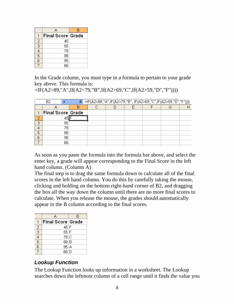
The first step in Excel is to create a spreadsheet with the final test scores entered in as shown below.

8

In the Grade column, you must type in a formula to pertain to your grade key above. This formula is: =IF(A2>89,"A",If(A2<79,”B”,If(A2>69,"C",If(A2>59,"D","F"))))

As soon as you paste the formula into the formula bar above, and select the enter key, a grade will appear corresponding to the Final Score in the left hand column. (Column A) The final step is to drag the same formula down to calculate all of the final scores in the left hand column. You do this by carefully taking the mouse, clicking and holding on the bottom right-hand corner of B2, and dragging the box all the way down the column until there are no more final scores to calculate. When you release the mouse, the grades should automatically appear in the B column according to the final scores.

Lookup Function The Lookup Function looks up information in a worksheet. The Lookup searches down the leftmost column of a cell range until it finds the value you

9

specify. When it finds the specified value, it then looks across the row and returns the value in the column you specify. The Lookup function works a lot like looking up a number in a phonebook: first you look down the phonebook until you find the person's name, then you look across to retrieve the person's phone number.

Plus and Minus Grading Scale An example of utilizing the Lookup Function is using the plus and minus grading scale. The first step would be to set up your Excel spreadsheet like the one below, placing the final score on the left and the Grade column on the right hand side.

Next, click one time on cell B2 and cut, paste the formula below in to the cell, and press Enter. =LOOKUP(A2,{0,60,63,67,70,73,77,80,83,87,90,93,97},{"F","D-","D","D+","C-","C","C+","B-","B","B+","A-","A","A+"}) This formula looks up the value in A2 (45) in the first row, finds the largest value that is less than or equal to it (60), and then returns the value in the last row that is in the same column (F). Next, click on the lower right hand corner of the cell B2 after the formula was pasted in to it, and slowly drag the lower corner all the way down until the end of your Final Scores. This will save time and automatically copy the same formulas in the rest of the cells.

10

Date and Time Functions

Date Function The Date Function returns the sequential serial number that represents a particular date.

If the year is between 1900 and 9999 Excel uses that value as the year. For example, DATE (2008, 1, 2) returns January 2, 2008.

The Date Function is very user-friendly. The first step when using the function is to make sure you click in the cell you would like the Date to actually appear. In this particular case, we have selected cell D2.

Once you have selected the cell, click on the function button located to the left side of the formula bar. Once the Insert Function box pops up, click on the drop down menu and select Date & Time as shown to the right. As soon as you hit the Ok button, another box pops up labeled Function Arguments as shown below.

11

Once this box pops up, click your cursor in the Year box, then click back on your Excel sheet, and click one time on your year. In this example we will click on the cell A2. Next do the same for the Month and the Day by clicking on the appropriate boxes. Once you have entered in all of your data, click on OK. Your Function Argument box disappears, and the date will appear in the appropriate cell. (D2).

Database Functions

DCOUNT function The DCOUNT function tallies the number of cells containing numbers. If you have a list or database, the database can be referenced as a cell reference or as a named range. The field is the number of the column in the database from left to right or the column heading in quotes (not case sensitive). The criteria are a range that contains the constraints the function operates from. For example, let's say you had a large database that had several blank cells as well as cells containing numbers, only some of which you were interested in. The criteria could specify to count all numbers having a value of more than 4,000 and less than 7,000. =DCOUNT(database,field,criteria) In our first example, we are going to look at the record of apple trees between a height of 10 and 16 and count how many of the Age fields in these records contain numbers.

12

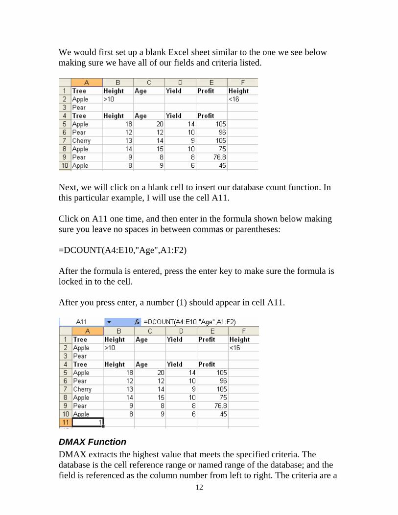
We would first set up a blank Excel sheet similar to the one we see below making sure we have all of our fields and criteria listed.

Next, we will click on a blank cell to insert our database count function. In this particular example, I will use the cell A11. Click on A11 one time, and then enter in the formula shown below making sure you leave no spaces in between commas or parentheses: =DCOUNT(A4:E10,"Age",A1:F2) After the formula is entered, press the enter key to make sure the formula is locked in to the cell. After you press enter, a number (1) should appear in cell A11.

DMAX Function DMAX extracts the highest value that meets the specified criteria. The database is the cell reference range or named range of the database; and the field is referenced as the column number from left to right. The criteria are a

13

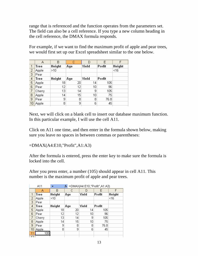
range that is referenced and the function operates from the parameters set. The field can also be a cell reference. If you type a new column heading in the cell reference, the DMAX formula responds. For example, if we want to find the maximum profit of apple and pear trees, we would first set up our Excel spreadsheet similar to the one below.

Next, we will click on a blank cell to insert our database maximum function. In this particular example, I will use the cell A11. Click on A11 one time, and then enter in the formula shown below, making sure you leave no spaces in between commas or parentheses: =DMAX(A4:E10,"Profit",A1:A3) After the formula is entered, press the enter key to make sure the formula is locked into the cell. After you press enter, a number (105) should appear in cell A11. This number is the maximum profit of apple and pear trees.

14

DMIN Function DMIN extracts the lowest value that meets the specified criteria. The DMIN function looks up the lowest value in a range or database. The database is the cell reference range or named range of the database, and the field is referenced as the column number from left to right. The criteria are a range that is referenced, and the function operates from the parameters set. The field can also be a cell reference. The DMIN function works the same way as the DMAX function only substituting DMIN in place of DMAX in the function. Please see DMAX for an example.

DSUM Function DSUM returns the total of the values that meet the specified criteria. =DSUM(database,field,criteria) The DSUM function operates much as the sum function, except that it operates on a database with criteria. The database is the named range of the database, and the field is referenced as the column number from left to right. The criteria are a range that is referenced, and the function operates from the parameters set. In our example below, we are going to find the total profit from apple trees with a height between 10 and 16 by using our database sum function. Below is an example of our Excel spreadsheet set up with various fields such as height, age, yield, profit, and height.

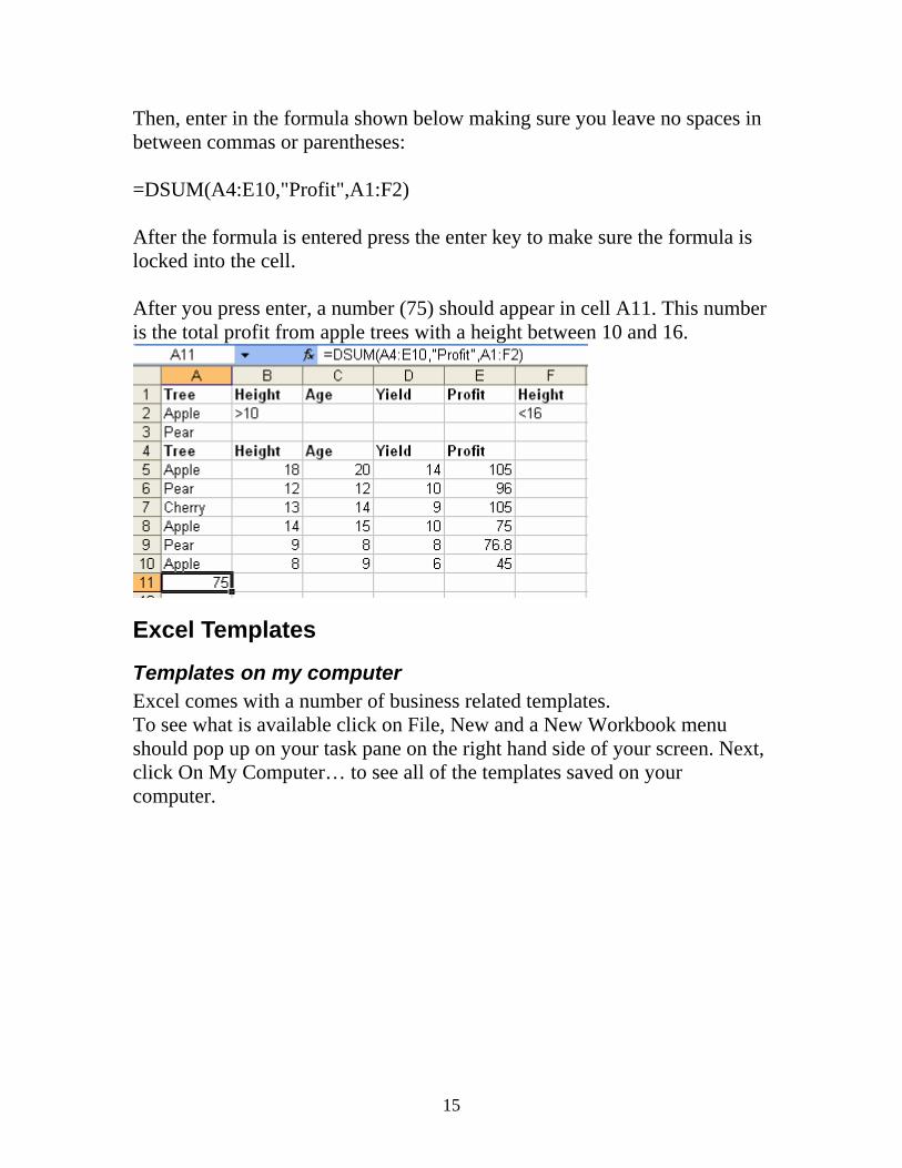
Next, we will click on a blank cell to insert our database sum function. In this particular example, click one time on the cell A11.

15

Then, enter in the formula shown below making sure you leave no spaces in between commas or parentheses: =DSUM(A4:E10,"Profit",A1:F2) After the formula is entered press the enter key to make sure the formula is locked into the cell. After you press enter, a number (75) should appear in cell A11. This number is the total profit from apple trees with a height between 10 and 16.

Excel Templates

Templates on my computer Excel comes with a number of business related templates. To see what is available click on File, New and a New Workbook menu should pop up on your task pane on the right hand side of your screen. Next, click On My Computer… to see all of the templates saved on your computer.

16

Once you click On My Computer… the template pop up box appears. Next, click on Spreadsheet Solutions to see more template options as shown below.

You can also create your own forms and save them as templates for further

17

use. The advantage of this is creating a unique document you can use on a recurring basis with the formatting, formulas, and style that you design. You can then use this document, i.e. template repeatedly. To save a document as a template, click on File and Save As. When the Save As window opens, put in a file name and choose ‘Document Template’ in the Save As Document Type area. This will save your document as a template.

Templates on Microsoft Office Online One of the newest features offered in Excel 2003 is their downloadable online templates. The only downfall from the online templates is that there is no way for the person to preview the template before downloading it on their personal computer; however, most of the templates are one-of-a-kind and a great tool to use in the work place. To see what is available, click on File, New, and a New Workbook menu should pop up on your task pane on the right hand side of your screen. Next, click on Templates on Office Online to see all of the templates Microsoft has to offer online.

Worksheets and Workbooks

Open Two Worksheets at Once Sometimes, you need to see two worksheets on the screen at the same time. Click the Window menu and select New Window. From the Window menu, select Arrange and choose Tile, Vertical. You will now have a split screen with two open worksheets visible. You can copy, move, and view both side by side.

18

Working with Multiple Worksheets To select multiple worksheets, hold down the Ctrl key as you click each tab. To select a contiguous group of worksheets, click the first one in the group, and then hold down the shift key and click the last one in the group. To select all the worksheets in the current workbook, right-click any worksheet tab and choose Select All sheets from the current shortcut menu. To quickly make any sheet active, click its index tab; to remove a sheet from a group, hold down the Ctrl key and click its tab. To remove the multiple selection and resume working with a single sheet, click any unselected sheet. If you have selected every sheet in the workbook, right-click any worksheet tab and choose Ungroup Sheets. If you have selected more than one sheet, you will see the word (Group) in brackets in the title bar, and any data you enter appears in the corresponding cells on each worksheet in the group. So, if you have grouped sheet1, sheet2, and sheet3, entering text in a cell A1 on sheet one will also enter the same text in the corresponding cells on sheet2 and sheet3.

19

Reviewing a Document Reviewing Toolbar Buttons:

To get the Reviewing Toolbar on your Screen for Microsoft Excel:

• Click on the View menu • Click on Toolbars • Click on Reviewing

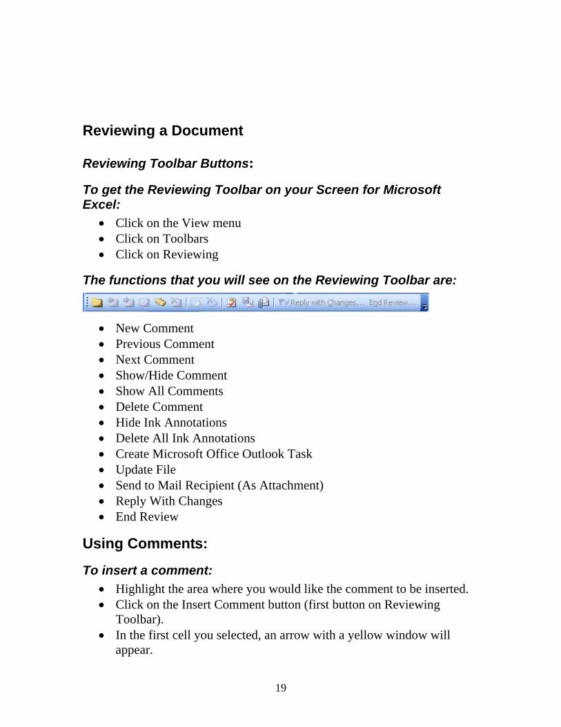
The functions that you will see on the Reviewing Toolbar are:

• New Comment • Previous Comment • Next Comment • Show/Hide Comment • Show All Comments • Delete Comment • Hide Ink Annotations • Delete All Ink Annotations • Create Microsoft Office Outlook Task • Update File • Send to Mail Recipient (As Attachment) • Reply With Changes • End Review

Using Comments:

To insert a comment: • Highlight the area where you would like the comment to be inserted. • Click on the Insert Comment button (first button on Reviewing

Toolbar). • In the first cell you selected, an arrow with a yellow window will

appear.

20

• In this window you can type in your comment or any ideas you may have.

• The comments made in the document will be numbered by the chronological order in which the comment is made.

• The comment that you are inserting will be the last one in the order. • Type the information that you want to insert.

Editing a Comment

• Put the cursor on the comment that you would like to edit. • Click on the Edit Comment button on the Reviewing Toolbar. • This will put the cursor on the comment that you want to edit, so you

can type in the corrections. • You can also edit other comments by clicking on the comment you

would like to edit and then clicking on Edit Comment button on the Reviewing Toolbar.

Previous Comment:

• By clicking on the Previous Comment button on the Reviewing Toolbar, you can move to the comment made before the one that you are currently viewing.

Next Comment:

• You can move to the next comment by clicking on Next Comment on the Reviewing Toolbar.

Delete the Comment:

• Click on the comment that you would like deleted, and then click on the Delete Comment button on the Reviewing Toolbar.

Tracking Changes:

• Each time you save a workbook, make sure to change tracking logs details about that workbook. You can use this history to understand what changes were made and to accept or reject revisions.

• This capability is particularly useful when several users edit a workbook. It's also useful when you submit a workbook to reviewers

21

for comments, and then want to merge input into one copy, selecting which changes and comments to keep.

Turn on change tracking for a workbook

• On the Tools menu, click Share Workbook, and then click the Editing tab.

• Select the “Allow changes by more than one user at the same time” check box.

• Click the Advanced tab. • Under Track changes, click Keep change history for, and in the Days

box, type the number of days of change history that you want to keep. • Be sure to enter a large-enough number of days because Microsoft

Excel permanently erases any change history older than this number of days.

• Click OK, and if prompted to save the file, click OK. • Turning on change tracking also shares the workbook, so multiple

users on a network can view and make changes at the same time.

View tracked changes

• On the Tools menu, point to Track Changes, and then click Highlight Changes. Make sure you are working in the original copy of your Excel Spreadsheet. If the Track changes while editing check box is not selected, Microsoft Excel has not recorded any change history for the workbook.

Select the Changes you want to see:

• To view all the changes that have been tracked, select the When check box and click All. Then, clear the Who and Where check boxes.

Changes made after a particular date

• Select the When check box, click Since Date, and then type the earliest date for which you want to view changes.

22

Changes made by a specific user

• Select the Who check box, and then click the user whose changes you want to view.

• Changes to a specific range of cells • Select the Where check box, and then enter a range reference, or

select a range on the worksheet.

Select how you want to view the changes

Highlight the worksheet

• Select the Highlight changes on screen check box. To view the details about a change, rest the pointer over a highlighted cell.

Listed on a separate sheet

• Select the List changes on a new sheet check box to display the History worksheet. This check box is available only after you have turned on change tracking and saved some changes.

Going to the Previous Change:

• Click on the Previous Change button in the Reviewing Toolbar.

Going to the Next Change:

• Click on the Next Change button in the Reviewing Toolbar.

Accept and reject changes

• On the Tools menu, point to Track Changes, and then click Accept or Reject Changes.

• If prompted to save the workbook, click OK.

Select the changes to review

23

Changes made after a particular date

• Select the When check box, click Since date, and then type the earliest date for which you want to review the changes.

Changes made by another user

• Select the Who check box, and then click the user whose changes you want to review.

Changes to a specific area

• Select the Where check box, and then enter a range reference, or select a range on the worksheet.

Changes to the entire workbook

• Clear the Where check box. • Click OK, and begin reviewing the information about each change in

the Accept or Reject Changes dialog box. The information includes other changes that are affected by the action you take for a change. You may need to scroll to see all of the information.

• To accept or reject each change, click Accept or Reject. The History worksheet records a rejection with "Undo" or "Result of rejected action" in the Action Type column.

• If prompted to select a value for a cell, click the value you want, and then click Accept.

• You must accept or reject a change before you can advance to the next change.

• You can accept or reject all remaining changes at once by clicking Accept All or Reject All.

Sending a Revised Document

• To send the revised version of the document, click on the Send to Mail Recipient button on the Reviewing Toolbar.

• An email message will appear with the document in it. • Fill out the address of the recipient, any text you would like to add

into the message, and click Send.

24

Printing

• To print a document with different versions and/or comments, click on the File menu and choose Print.

• Here you have several options in the “Print what:” area at the bottom of the window:

• You can just print the Document • You can just print the Comments • OR You can click on Options... In the “include with document”

section, you can click on the box for Comments to print the comments with the document