examples - iqcciqc.udg.edu/~marcel/workshop/manuals/adf/examples.pdf · nno: core-electron binding...
TRANSCRIPT

ExamplesADF Program System
Release 2010
Scientific Computing & Modelling NVVrije Universiteit, Theoretical ChemistryDe Boelelaan 1083; 1081 HV Amsterdam; The NetherlandsE-mail: [email protected]
Copyright © 1993-2010: SCM / Vrije Universiteit, Theoretical Chemistry, Amsterdam, The NetherlandsAll rights reserved
1

Table of ContentsExamples......................................................................................................................................................... 1Table of Contents ........................................................................................................................................... 2General notes on the Examples .................................................................................................................... 5Model Hamiltonians........................................................................................................................................ 8
Special exchange-correlation functionals .......................................................................................... 8CO: asymptotically correct XC potentials ....................................................................................... 8OH: Meta-GGA energy functionals................................................................................................. 9H: SIC-VWN potential................................................................................................................... 11HI: Hartree-Fock........................................................................................................................... 11H2PO: B3LYP............................................................................................................................... 13MM Dispersion: Molecular Mechanics dispersion-corrected functionals ...................................... 14
ZORA and spin-orbit Relativistic Effects .......................................................................................... 17Au2: ZORA Relativistic Effects ..................................................................................................... 17Bi and Bi2: Spin-Orbit ................................................................................................................... 19Tl: Spin-Orbit unrestricted non-collinear ....................................................................................... 24AuH: excitation energies including spin-orbit coupling ................................................................. 24
Solvents, other environments ............................................................................................................ 26HCl: COSMO................................................................................................................................ 26Glycine: 3D-RISM......................................................................................................................... 27N2 and PtCO: Electric Field, Point Charge(s), use of Basis keyword .......................................... 29FDE: Frozen Density Embedding ................................................................................................. 31
H2O in water: FDE............................................................................................................... 31HeCO2: FDE freeze-and-thaw............................................................................................. 33NH3-H2O: FDE energy ........................................................................................................ 37Ne-H2O: FDE energy, unrestricted fragments..................................................................... 39H2O-Li(+): FDE geometry optimization................................................................................ 40NH3-H2O: FDE geometry optimization ................................................................................ 41Acetonitrile in water: FDE NMR shielding ........................................................................... 42Subsystem TDDFT, coupled FDE excitation energies ........................................................ 44
QM/MM calculations ..................................................................................................................... 48pdb2adf: transforms a PDB file in a QM/MM adf-input file .................................................. 48QMMM_Butane: Basic QMMM Illustration .......................................................................... 50QMMM_CYT........................................................................................................................ 52QMMM_Surface: Ziegler-Natta catalysis............................................................................. 54
Structure and Reactivity .............................................................................................................................. 58Geometry Optimizations..................................................................................................................... 58
H2O: Geometry Optimization........................................................................................................ 58Formaldehyde: another Optimization ........................................................................................... 61Aspirin: an optimization in delocalized coordinates ...................................................................... 62AuH: Scalar-Relativistic Optimization ........................................................................................... 63H2O: restraint Geometry Optimization.......................................................................................... 64H2O: constraint Geometry Optimization ....................................................................................... 66LiF: optimization with an external electric field or point charges .................................................. 68CH2O: excited state geometry optimization with a constraint ...................................................... 69
Transition States, Linear Transits, Intrinsic Reaction Coordinates ............................................... 70HCN: LT, Frequencies, TS, and IRC............................................................................................ 70HCN: transition state search with the CINEB method .................................................................. 78C2H6 internal rotation: TS search using partial Hessian.............................................................. 79CH4+HgCl2⇔CH3HgCl+HCl: a TS search ................................................................................... 81F-+CH3Cl: TS reaction coordinate................................................................................................ 84H2O: constraint Linear Transit ...................................................................................................... 84H2O: (non-)Linear Transit ............................................................................................................. 85
Quild ..................................................................................................................................................... 86CO: Quild B3LYP geometry optimization ..................................................................................... 86
2

H2O dimer: Quild QM/MM geometry optimization ........................................................................ 88F- + CH3Cl: Quild transition state search ..................................................................................... 90
DFTB..................................................................................................................................................... 91Aspirin: DFTB geometry optimization ........................................................................................... 91CH3CN_3H2O: DFTB frequency calculation................................................................................ 92
Total energy, Multiplet States, S2, Localized hole, CEBE................................................................ 92H2O: Total Energy calculation ...................................................................................................... 92[Cr(NH3)6]3+: Multiplet States....................................................................................................... 93CuH+: calculation of S2 ................................................................................................................ 98N2+: Localized Hole...................................................................................................................... 98Fe4S4: broken spin-symmetry ...................................................................................................... 99NNO: Core-electron binding energies ........................................................................................ 101
Spectroscopic Properties .......................................................................................................................... 105IR Frequencies, (resonance) Raman, VROA, VCD, Franck-Condon factors................................ 105
NH3: Numerical Frequencies...................................................................................................... 105UF6: Numerical Frequencies, spin-orbit coupled ZORA............................................................. 108H2O: Numerical Frequencies, accurate Hartree-Fock................................................................ 109PH2: Numerical Frequencies of an excited state........................................................................ 111CN: Analytic Frequencies ........................................................................................................... 112CH4: Analytic Frequencies ......................................................................................................... 113HI: Analytic Frequencies, scalar ZORA...................................................................................... 114Ethanol: mobile block Hessian ................................................................................................... 115CH4: mobile block Hessian......................................................................................................... 117NH3: Raman ............................................................................................................................... 118HF: Resonance Raman, excited state finite lifetime................................................................... 120Uracil: Resonance Raman, excited state gradient ..................................................................... 120H2O2: vibrational Raman optical activity (VROA)....................................................................... 122H2O2: resonance VROA............................................................................................................. 123NHDT: Vibrational Circular Dichroism ........................................................................................ 124NO2: Franck-Condon Factors..................................................................................................... 125
Time-dependent DFT applications................................................................................................... 128Au2: Response Properties.......................................................................................................... 128CN: excitation energies open shell molecule ............................................................................. 129SiH2: spin-flip excitation energies............................................................................................... 130N2: TDHF excitation energies..................................................................................................... 131TiCl4: core excitation energies ................................................................................................... 132Ne: (core) excitation energies including spin-orbit coupling ....................................................... 134AgI: excitation energies including spin-orbit coupling perturbatively .......................................... 135N2: excited state geometry optimization..................................................................................... 136CH2: spin-flip excited state geometry optimization..................................................................... 137Hyperpol: Hyperpolarizabilities of He and H2 ............................................................................. 138AgI: polarizabilities including spin-orbit coupling ........................................................................ 140HF: Dispersion Coefficients ........................................................................................................ 140DMO: Circular Dichroism spectrum............................................................................................ 141Twisted Ethene: CD spectrum, hybrid functional ....................................................................... 142DMO: Optical Rotation Dispersion ............................................................................................. 144DMO: ORD, lifetime effects (key AORESPONSE) ..................................................................... 145Propene: damped Verdet constants ........................................................................................... 146H2O: Verdet constants ............................................................................................................... 147H2O: MCD ................................................................................................................................. 148H2O: static magnetizability ......................................................................................................... 148H2O: dynamic magnetizability .................................................................................................... 149C2H4: Time-dependent current-density-functional theory .......................................................... 150
NMR chemical shifts and spin-spin coupling constants ............................................................... 151HBr: NMR Chemical Shifts ......................................................................................................... 151HgMeBr: NMR Chemical Shifts .................................................................................................. 152CH4: NMR Chemical Shifts, SAOP potential .............................................................................. 153
3

CO: NMR Chemical Shifts, SIC-VWN potential.......................................................................... 154PF3: NMR Properties, Nucleus-independent chemical shifts ..................................................... 155PF3: Comparison of NMR with EPR/NMR.................................................................................. 156PF3: NMR with B3LYP ............................................................................................................... 157VOCl3: NMR Chemical shifts...................................................................................................... 158C2H2: NMR Spin-spin coupling constants .................................................................................. 159HF: NMR Spin-spin coupling constants, hybrid PBE0................................................................ 161PbH4: NMR Spin-spin coupling constants, finite nucleus........................................................... 162
ESR / EPR properties ........................................................................................................................ 164TiF3: ESR g-tensor, A-tensor, Q-tensor ..................................................................................... 164VO: collinear approximation, ESR g-tensor, A-tensor, Q-tensor ................................................ 169Ge+ and H2+: ESR g-tensor (epr program) ................................................................................ 171NF2: spin-other-orbit contribution g-tensor ................................................................................. 172
EFG, Mössbauer ................................................................................................................................ 173Ferrocene: Mössbauer spectroscopy ......................................................................................... 173
Analysis....................................................................................................................................................... 175Fragment orbitals and bond energy decomposition...................................................................... 175
Ni(CO)4: Compound Fragments................................................................................................. 175PtCl4H22-: Fragments again ....................................................................................................... 177H2: Spin-unrestricted Fragments................................................................................................ 181PCCP: Bond Energy analysis open-shell fragments .................................................................. 184TlH: Spin-Orbit SFO analysis ..................................................................................................... 187Bader Analysis (AIM).................................................................................................................. 190Bond Orders ............................................................................................................................... 191NOCV: ethylene -- Ni-diimina & H+ -- CO................................................................................... 191NOCV: CH2 -- Cr(CO)5............................................................................................................... 194NOCV: CH3 -- CH3 ..................................................................................................................... 195
Post-ADF analysis utilities ............................................................................................................... 198NO2: Contour Plots using Densf and Cntrs ................................................................................ 198C2H2: Localization of Molecular Orbitals .................................................................................... 200Cu4CO: Density of States........................................................................................................... 203
Charge transfer integrals (transport properties) ............................................................................ 205AT base pair: Charge transfer integrals ..................................................................................... 205
Third party analysis software........................................................................................................... 208adf2aim: convert an ADF TAPE21 to WFN format (for Bader analysis) .................................... 208NBO analysis: adfnbo, gennbo................................................................................................... 208NBO analysis: EFG .................................................................................................................... 210NBO analysis: NMR chemical shift............................................................................................. 212NBO analysis: NMR spin-spin coupling...................................................................................... 213
Accuracy ..................................................................................................................................................... 216BSSE, SCF convergence, Frequencies ........................................................................................... 216
Cr(CO)5+CO: Basis Set Superposition Error.............................................................................. 216Ti2O4: troubleshooting SCF convergence .................................................................................. 221NH3: rescan frequencies ............................................................................................................ 223
Scripting...................................................................................................................................................... 225Prepare an ADF job and generate a report ..................................................................................... 225
Bakerset: GO optimization for multiple xyz files ......................................................................... 225Methane: basis set and integration accuracy convergence test................................................. 225
List of examples ......................................................................................................................................... 227
4

General notes on the ExamplesThe ADF package contains a series of sample runs. Provided are UNIX scripts to run the calculations andthe resulting output files. In most directories, there are also files for ADFinput present.
The examples serve:
• To check that the program has been installed correctly:run the sample inputs and compare the results with the provided outputs.Read the remarks below about such comparisons.
• To demonstrate how to do calculations: an illustration to the User manuals.The number of options available in ADF is substantial and the sample runs do not cover all ofthem.They should be sufficient, however, to get a feeling for how to explore the possibilities.
• To work out special applications that do not fit well in the User's Guide.
Where references are made to the operating system (OS) and to the file system on your computer,the terminology of a UNIX type OS is used and a hierarchical structure of directories is assumed.
All sample files are stored in subdirectories under $ADFHOME/examples/, where $ADFHOME is the maindirectory of the ADF package. There are two main subdirectories in examples/: adf/ for calculations with themolecular code ADF (and related utility programs) and band/ for calculations with the periodic structurescode BAND. Each sample run has its own directory (under adf/ or band/ respectively). For instance,$ADFHOME/examples/adf/HCN/ contains an ADF calculation on the HCN molecule. Each samplesubdirectory contains:
• A file TestName.run: the UNIX script to execute the calculation or sequence of calculationsof the example
• A file TestName_orig.out: the resulting output(s) against which you can compare the outcomeof your own calculation.
• Zero or more files with a .adf extension. These files, if present, are intended for ADFinputand demonstrate the same functionality as the two files above. However, there are alsodifferences between the .adf and the TestName.run files so the results obtained with the.adf files cannot be compared directly with TestName_orig.out. Also, the TestName.runfile usually contains more than one calculation, for which more than one .adf file isrequired. That's why in some directories you may find more than one .adf file.In some directories, there are no .adf files, which usually means the functionality demonstrated bythe example is not supported by the GUI.
Notes:
• Running the examples on Windows:You can run an example calculation by double-clicking on the appropriate .run file.After the calculation has finished, you can compare the TestName.out file with thereference TestName_orig.out file. See remarks about comparing output files below.
• The UNIX scripts make use of the rm (remove) command. Some UNIX users may have aliasedthe rm command. They should accordingly adapt these commands in the sample scripts soas to make sure that the scripts will remove the files.New users may get stuck initially because of files that are lingering aroundafter an earlier attempt to run one of the examples. In a subsequent run, whenthe program tries to open a similar (temporary or result) file again, an error may occur ifsuch a file already exists. Always make sure that no files are left in therun-directory except those that are required specifically.
• It is a good idea to run each example in a separate directory that contains no other important files.• The run-scripts use the environment variables ADFBIN and ADFRESOURCES.
They stand respectively for the directory that contains the program executables and the maindirectory of the database. To use the scripts as they are you must have defined the variables
5

ADFBIN and ADFRESOURCES in your environment.If a parallel (PVM or MPI) version has been installed, it is preferable to have also theenvironment variable NSCM. This defines the default number of parallel processes that theprogram will try to use. Consult the Installation Manual for details.
• As you will note the sample run scripts refer to the programs by names like 'adf', 'band',and so on. When you inspect your $ADFBIN directory, however, you may findthat the program executables have names 'adf.exe', 'band.exe'.There are also files in $ADFBIN with names 'adf', 'band', but these are in fact scripts to executethe binaries. We strongly recommend that you use these scripts in your calculations, inparticular when running parallel jobs: the scripts take care of some aspectsthat you have to do otherwise yourself in each calculation.
• You need a license file to run any calculations successfully. If you have troubles with your licensefile, consult the Installation manual. If that doesn't help contact us at [email protected]
Many of the provided samples have been devised to be short and simple, at the expense of physical orchemical relevance and precision or general quality of results. They serve primarily to illustrate the use ofinput, necessary files, and type of results. The descriptions have been kept brief. Extensive informationabout using keywords in input and their implications is given in the User's Guides (ADF and BAND) and theUtilities, Analysis, and Property Programs documents (NMR, DIRAC, and other utility programs).
When you compare your own results with the sample outputs, you should check in particular (as far asapplicable):
• Occupation numbers and energies of the one-electron orbitals;• The optimized geometry;• Vibrational frequencies;• The bonding energy and the various terms in which it has been decomposed;• The dipole moment;• The logfile. At the end of a calculation the logfile is automatically appended
(by the program itself) to the standard output.
General remarks about comparisons:
• For technical reasons, discussion of which is beyond the scope of this document, differencesbetweenresults obtained on different machines, or with different numbers of parallel processes, may bemuchlarger than you would expect. They may significantly exceed the machine precision. What youshouldcheck is that they fall well (by at least an order of magnitude) within the numericalintegration precision used in the calculation.
• For similar reasons the orientation of the molecule used by the program may be different ondifferentmachines, even when the same input is supplied. In such cases the different orientations shouldbe relatedand only differ in some trivial way, such as by a simple rotation of all coordinates by 90 degreesaround the z-axis. When in doubt, contact an ADF representative.
• An ADF run may generate, apart from result files that you may want to save, a few scratch files.The UNIX scripts that run the samples take care of removing these files after the calculations havefinished, to avoid that the program aborts in the next run by attempting to open a 'new' file that isfound to exist already.
• A sample calculation may use one or more data files, in particular fragment files. The samplesare self-contained: they first run the necessary pre-calculations to produce the fragment files.In 'normal' research work you may have libraries of fragments available, first for the 'basic atoms',and later, as projects are developing, also for larger fragments so that you can start immediatelyonthe actual system by attaching the appropriate fragment files.
6

Default settings of print options result in a considerable amount of output. This is also the case in some ofthe sample runs, although in many of them quite a bit of 'standard' output is suppressed by insertingapplicable print control keys in the input file. Consult the User's Guide about how to regulate input with keysin the input file.
Survey of the Examples
The Survey of Applications follows a survey of the main application topics with references to related sampleruns is given. A sample run usually involves several calculations, for instance a few CREATE runs (withADF), then a molecular calculation (also ADF), and finally a NMR calculation (with the NMR program) tocompute chemical shifts. The samples are identified in this documentation by the name of the directory theyreside in. The samples are indicated by these directory names. For instance, GO_H2O refers to thedirectory GO_H2O/ (in $ADFHOME/adf/), where in this case GO stands for Geometry Optimization.
7

Model Hamiltonians
Special exchange-correlation functionals
CO: asymptotically correct XC potentials
Sample directory adf/CO_model
For property calculations, xc potentials with asymptotically correct (-1/r) behavior outside the molecule, theresults tend to be superior to regular LDA or GGA calculations. This is especially true for small moleculesand for properties that depend heavily on the proper description of the outer region of the molecule. In theexample, all-electron basis sets are used. This is mandatory for the SAOP potential.
$ADFBIN/adf -n1 <<EORcreate C $ADFRESOURCES/TZ2P/Cend inputEORmv TAPE21 t21.C
$ADFBIN/adf -n1 <<EORcreate O $ADFRESOURCES/TZ2P/Oend inputEORmv TAPE21 t21.O
In the next example, excitation energies are calculated with the GRACLB potential. This potential requiresone number as argument: the experimental ionization potential in atomic units. This number can be eitherbased on an experimental value, or on previous GGA total energy calculations.
$ADFBIN/adf <<EORtitle CO excitations grac potential
INTEGRATION 6.0
XCModel GRACLB 0.515
End
AtomsO 0 0 0C 1.128205364 0 0end
ExcitationLowest 10Onlysing
End
FragmentsO t21.OC t21.C
End
8

end inputEOR
rm TAPE21 logfile
The same calculation with the SAOP xc potential would differ in the XC block only:
XCModel SAOP
End
SAOP depends on the orbitals which makes it more expensive to evaluate than GRAC for large molecules.
OH: Meta-GGA energy functionals
Sample directory adf/OH_MetaGGA
First two calculations on OH are performed which use, respectiveley, the hybrid meta-GGA TPSSh and themeta-GGA TPPS during the SCF. They require, respectively, the following XC input:
XCMetaHybrid TPSSh
ENDXCMetaGGA TPSS
END
Next large even-tempered basis sets are used in the calculation of the atomization energy of OH usingvarious modern GGA, meta-GGA and hybrid post-SCF energy expressions.
In the Create runs, a large even-tempered basis set is selected for O and H, which should give results closerto the basis set limit than the regular ADF basis sets. For both atoms, a second atomic calculation followsthe Create run, in order to enable a comparison to the true atoms, rather than the artificial sphericallysymmetric atom from the Create run. This is achieved by specifying the keywords
unrestrictedcharge 0 2symmetry C(lin)occupationssigma 3 // 3pi 2 // 0end
in the case of oxygen. This fixes the proper occupations. The result files of both the Create runs and theatomic correction runs are stored.
In the molecular calculation, the symmetry of the molecule is explicitly broken and the occupations arespecified in order to avoid the fractional occupations that ADF would otherwise choose. Although it is notsaid that such a solution would be inferior, the integer occupation solution is the one which allows directcomparison to literature results obtained with other programs.
One of the new GGA potentials has been specified for the xc potential and the keyword METAGGA impliesthat a series of GGA and meta-GGA xc energies is to be calculated and compared to those energies from
9

the atomic calculations. Specifying HARTREEFOCK also enables calculation of PostSCF energies usinghybrid functionals.
METAGGAsymmetry C(lin)xcGGA PBEendHARTREEFOCK
A fairly high numerical integration has been specified. For meta-GGA calculations we do recommend this, atleast 6 for the time being, as the numerical stability of the results tends to be somewhat lower than forregular GGA calculations.
The block key ENERGYFRAG
ENERGYFRAGO t21.unr.OH t21.unr.HEND
implies that the meta-GGA result must not only be compared to the spherically symmetric results from theCreate runs, but also to the non-spherical atoms.
The molecular output file prints the PBE Total Bonding energy as usual (in various energy units).
Then a prints a list of 'Total Bonding Energies' for many different Exc functionals, including PBE. Becausethe numerical approach to obtain the two PBE results is somewhat different, small differences may occurbetween the two numbers. You now have an overview of the bonding energies of all (meta)GGA functionalscurrently implemented in ADF. This should give a good indication of the theoretical error bar or theuncertainty in the xc approximation.
Total Bonding Energy: -0.286127457276205 -7.7859 -179.55-751.23TOTAL BONDING ENERGIES FROM VARIOUS XC FUNCTIONALSwith respect to fragments in FRAGMENTS input block
hartree eV kcal/mol kJ/molTotal Bonding Energy with respect to FRAGMENTS
XC Energy Functional====================FR: KCIS-modified [1] = -0.2755742057 -7.4987587362 -172.9254430523 -723.5200549587FR: KCIS-original [2] = -0.2777894828 -7.5590395194 -174.3155506035 -729.3362649626FR: PKZB [3] = -0.2815570432 -7.6615600946 -176.6797306630 -739.2279943483FR: VS98 [4] = -0.3017049511 -8.2098127875 -189.3227350810 -792.1263249228FR: LDA(VWN) [5] = -0.2887564297 -7.8574654492 -181.1974143810 -758.1299830563FR: PW91 [6] = -0.2876922977 -7.8285089331 -180.5296614163 -755.3361046473FR: BLYP [7] = -0.2770745036 -7.5395839361 -173.8668943006 -727.4590869882FR: BP [8] = -0.2855241909 -7.7695117221 -179.1691537365 -749.6437405057FR: PBE [9] = -0.2858734106 -7.7790144775 -179.3882924288 -750.5606167957.....
The same energy comparison is done with respect to the fragments (which most currently be atomic) in theENERGYFRAG block. These are the numbers which should be comparable to experimental numbers.
Finally, the references for the various Exc functionals are printed in the output file.
XC Energy Functional====================EF: KCIS-modified [1] = -0.1713622482 -4.6630059333 -107.5314455812 -449.9115690750EF: KCIS-original [2] = -0.1701706820 -4.6305817515 -106.7837263654 -446.7831118709EF: PKZB [3] = -0.1716508948 -4.6708604097 -107.7125740668 -450.6694106602EF: VS98 [4] = -0.1712676117 -4.6604307410 -107.4720602503 -449.6631008503EF: LDA(VWN) [5] = -0.1980694328 -5.3897456994 -124.2904587006 -520.0312800855EF: PW91 [6] = -0.1759694023 -4.7883730257 -110.4224787188 -462.0076517434EF: BLYP [7] = -0.1748768123 -4.7586421272 -109.7368680765 -459.1390568111
10

EF: BP [8] = -0.1785853781 -4.8595573769 -112.0640284617 -468.8758958794EF: PBE [9] = -0.1751227104 -4.7653333576 -109.8911714787 -459.7846622469....
Similar calculations can be done to obtain energy differences between different molecules. In that case theENERGYFRAG keyword is not operational though. No detailed breakdown of the bonding energy iscurrently available for these new energy functionals. Experience shows that the energy values depend onlymildly on the chosen xc functional for the xc potential.
H: SIC-VWN potential
Sample directories: adf/H_SICVWN/
Computation of the hydrogen atom with the SIC-VWN potential, should give the exact result (E=-0.5 a.u.).
Note: adf with the SIC-VWN only runs correctly serial, and symmetry NOSYM is required.
$ADFBIN/adf -n1 << eorTITLE H atom, SIC-VWN (should be exact)SYMMETRY NOSYMUNRESTRICTEDCHARGE 0 1ATOMS
1 H 0.0000 0.0000 0.0000ENDINTEGRATION 6.0 6.0FRAGMENTS
H t21.HENDXC
LDA VWNENDSICOEP
IPRINT 1SELF 35
ENDDEPENDENCY fit=1e-10 bas=1e-8SINGULARFIT FRUGALEND INPUTeor
HI: Hartree-Fock
Sample directory: adf/HI_EFG/
Example shows a Hartree-Fock calculation with a non-relativistic, scalar relativistic ZORA, and a spin-orbitcoupled ZORA Hamiltonian. In this case ADF also calculates the electric field gradient (EFG) at the H and Inuclei (keyword QTENS).
First the non-relativistic calculation. Note that in this case the all-electron basis sets are obtained from the$ADFRESOURCES/ZORA directory.
11

$ADFBIN/adf << eorAtomsH 0 0 0I 0 0 1.609
Endqtensxchartreefock
endintegration 5BasisType ZORA/TZ2PCore None
EndEnd inputeor
Next the scalar relativistic ZORA calculation. Note that in this case the all-electron basis sets are alsoobtained from the $ADFRESOURCES/ZORA directory, but this is default place where the key BASIS willsearch for basis sets in case of ZORA. ADF will also calculate the EFG including the small componentdensity, also called SR ZORA-4.
$ADFBIN/adf << eorAtomsH 0 0 0I 0 0 1.609
Endqtensxchartreefock
endRelativistic Scalar ZORAintegration 5BasisType TZ2PCore None
EndEnd inputeor
Next the spin-orbit coupled relativistic ZORA calculation. Note that in this case the all-electron basis sets arealso obtained from the $ADFRESOURCES/ZORA directory, but again this is default place where the keyBASIS will search for basis sets in case of ZORA. If one calculates this molecule with symmetry nosym,ADF will also calculate the EFG including the small component density, also called ZORA-4.
$ADFBIN/adf << eorAtomsH 0 0 0I 0 0 1.609
Endqtensxchartreefock
endRelativistic Spinorbit ZORAsymmetry nosymintegration 5
12

BasisType TZ2PCore None
EndEnd inputeor
H2PO: B3LYP
Sample directory: adf/H2PO_B3LYP/
Example shows an unrestricted B3LYP calculation. In this case ADF also calculates the hyperfineinteractions at H, P, and O nuclei (keyword ESR).
The 'DEPENDENCY' key is set to 1e-4. Note that for hybrids and Hartree-Fock the dependency key isalways set. The default value in that case is 4e-3. By explicitely setting the 'DEPENDENCY' key we can usea lower value, which is possible in this case. One should check that the results remain reliable if one uses asmaller value for the 'DEPENDENCY' key.
$ADFBIN/adf << eorTitle hfs H2PO B3LYP TZ2PAtoms
O 1.492 0.000 0.000P 0.000 0.000 0.000H -0.600 -0.650 1.100H -0.600 -0.650 -1.100
Endxchybrid B3LYP
endBasisType TZ2PCore None
Enddependency bas=1e-4integration 5esrendunrestrictedcharge 0 1end inputeor
For the hyperfine interactions it is important to use all-electron basis sets on the interesting nuclei. One canget more accurate results if one uses a larger basis set, like the QZ4P basis set, which is present in the$ADFRESOURCES/ZORA directory. The Basis key should then be:
BasisType ZORA/QZ4PCore None
End
The QZ4P results for the isotropic value of the A-tensor are approximately: -24.77 MHz for 17O, 962.02 MHzfor 31P, and 110.72 MHz for 1H.
13

You may want to compare the results with previous B3LYP results by N. R. Brinkmann and I. Carmichael, J.Phys. Chem. A (2004), 108, 9390-9399, which give for the Isotropic Fermi Contact Couplings (MHz) for the2A' State of H2PO using B3LYP, with an aug-cc-pCVQZ basis set: -24.24 MHz for 17O, 963.33 MHz for 31P,and 111.51 MHz for 1H.
MM Dispersion: Molecular Mechanics dispersion-corrected functionals
Sample directory: adf/MM_Dispersion/
Summary:
• MM dispersion (old implementation)• Dispersion-corrected GGA-D functionals
MM dispersion (old implementation)
First example shows a geometry optimization of a van der Waals complex of two benzene molecules,connected to each other with a hydrogen molecule. With the MMDISPERSION keyword an extra empiricalforce (of similar form as in molecular mechanics) is added to the interaction between the three fragments,where one benzen molecule is fragment 1 (FD=1), the other benzene molecule is fragment 2 (FD=2), andthe hydrogen molecule is fragment 3 (FD=3).
The atomic parameters are read from the file $ADFRESOURCES/MMDispersion/disp-param. The PBEfunctional and the TZP basis set are used, which is necessary if one wants to use the TZ parameters for thedamping function, which are optimized for this combination of functional and basis set.
$ADFBIN/adf << eorbasis
type TZPcore small
EndXC
GGA PBEEndgeometry
converge grad=0.001iterations 5
endIntegration 4.5SCF
Iterations 60Converge 1.0E-06 1.0E-6
Endmmdispersion
damping sigmdamp_param tzcombi s-kfile_name $ADFRESOURCES/MMDispersion/disp-paramnodefault
endnoprint sfoAtoms cartesiansC.ctr 0.000000000000 3.050000000000 1.391500000000 FD=1
14

H.h 0.000000000000 3.050000000000 2.471500000000 FD=1C.ctr 1.205074349366 3.050000000000 0.695750000000 FD=1H.h 2.140381785453 3.050000000000 1.235750000000 FD=1C.ctr 1.205074349366 3.050000000000 -0.695750000000 FD=1H.h 2.140381785453 3.050000000000 -1.235750000000 FD=1C.ctr -0.000000000000 3.050000000000 -1.391500000000 FD=1H.h -0.000000000000 3.050000000000 -2.471500000000 FD=1C.ctr -1.205074349366 3.050000000000 -0.695750000000 FD=1H.h -2.140381785453 3.050000000000 -1.235750000000 FD=1C.ctr -1.205074349366 3.050000000000 0.695750000000 FD=1H.h -2.140381785453 3.050000000000 1.235750000000 FD=1C.ctr -1.205074349366 -3.050000000000 -0.695750000000 FD=2H.h -2.140381785453 -3.050000000000 -1.235750000000 FD=2C.ctr -0.000000000000 -3.050000000000 -1.391500000000 FD=2H.h -0.000000000000 -3.050000000000 -2.471500000000 FD=2C.ctr 1.205074349366 -3.050000000000 -0.695750000000 FD=2H.h 2.140381785453 -3.050000000000 -1.235750000000 FD=2C.ctr 1.205074349366 -3.050000000000 0.695750000000 FD=2H.h 2.140381785453 -3.050000000000 1.235750000000 FD=2C.ctr -0.000000000000 -3.050000000000 1.391500000000 FD=2H.h -0.000000000000 -3.050000000000 2.471500000000 FD=2C.ctr -1.205074349366 -3.050000000000 0.695750000000 FD=2H.h -2.140381785453 -3.050000000000 1.235750000000 FD=2H.h 0.0 0.35 0.0 FD=3H.h 0.0 -0.35 0.0 FD=3EndEnd Input
The part of the bond energy that is due to the Grimme dispersion corrected functional is only inter-molecular(atom-atom contributions for which the fragment numbers FD are different).
Dispersion-corrected GGA-D functionals
In the second example a structure with 2 benzene molecules and a hydrogen molecule is optimized with theGrimme dispersion corrected PBE. Needed is the subkey DISPERSION in the key XC. If one starts withatomic fragments the part of the bond energy that is due to the Grimme dispersion corrected functional isboth inter-molecular as well as intra-molecular. In this case the subargument FD= in the ATOMS block keyword is not used, which was only used in the old MM dispersion calculation.
$ADFBIN/adf << eorTitle Geometry optimization with Grimme dispersion correction for GGAbasis
type TZPcore small
EndXC
GGA PBEDISPERSION
Endgeometry
converge grad=0.001Branch OLDiterations 50
endIntegration 4.5Atoms cartesians
15
C 0.000000000000 3.050000000000 1.391500000000H 0.000000000000 3.050000000000 2.471500000000C 1.205074349366 3.050000000000 0.695750000000H 2.140381785453 3.050000000000 1.235750000000C 1.205074349366 3.050000000000 -0.695750000000H 2.140381785453 3.050000000000 -1.235750000000C -0.000000000000 3.050000000000 -1.391500000000H -0.000000000000 3.050000000000 -2.471500000000C -1.205074349366 3.050000000000 -0.695750000000H -2.140381785453 3.050000000000 -1.235750000000C -1.205074349366 3.050000000000 0.695750000000H -2.140381785453 3.050000000000 1.235750000000C -1.205074349366 -3.050000000000 -0.695750000000H -2.140381785453 -3.050000000000 -1.235750000000C -0.000000000000 -3.050000000000 -1.391500000000H -0.000000000000 -3.050000000000 -2.471500000000C 1.205074349366 -3.050000000000 -0.695750000000H 2.140381785453 -3.050000000000 -1.235750000000C 1.205074349366 -3.050000000000 0.695750000000H 2.140381785453 -3.050000000000 1.235750000000C -0.000000000000 -3.050000000000 1.391500000000H -0.000000000000 -3.050000000000 2.471500000000C -1.205074349366 -3.050000000000 0.695750000000H -2.140381785453 -3.050000000000 1.235750000000H 0.0 0.35 0.0H 0.0 -0.35 0.0EndEnd Input
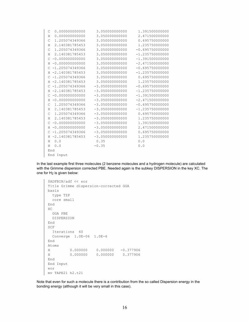
In the last example first three molecules (2 benzene molecules and a hydrogen molecule) are calculatedwith the Grimme dispersion corrected PBE. Needed again is the subkey DISPERSION in the key XC. Theone for H2 is given below:
$ADFBIN/adf << eorTitle Grimme dispersion-corrected GGAbasis
type TZPcore small
EndXC
GGA PBEDISPERSION
EndSCF
Iterations 60Converge 1.0E-06 1.0E-6
EndAtomsH 0.000000 0.000000 -0.377906H 0.000000 0.000000 0.377906EndEnd Inputeormv TAPE21 h2.t21
Note that even for such a molecule there is a contribution from the so called Dispersion energy in thebonding energy (although it will be very small in this case).
16

Next a structure is calculated in which the three calculated molecules in it. If one starts with molecularfragments the part of the bond energy that is due to the Grimme dispersion corrected functional is only inter-molecular.
$ADFBIN/adf << eorTitle Grimme dispersion-corrected GGAFragments
b1 benzene1.t21b2 benzene2.t21h2 h2.t21
EndXC
GGA PBEDISPERSION
EndAtomsC 0.000000 1.398973 -3.054539 f=b1H 0.000000 2.490908 -3.049828 f=b1C 1.211546 0.699486 -3.054539 f=b1H 2.157190 1.245454 -3.049828 f=b1C 1.211546 -0.699486 -3.054539 f=b1H 2.157190 -1.245454 -3.049828 f=b1C 0.000000 -1.398973 -3.054539 f=b1H 0.000000 -2.490908 -3.049828 f=b1C -1.211546 -0.699486 -3.054539 f=b1H -2.157190 -1.245454 -3.049828 f=b1C -1.211546 0.699486 -3.054539 f=b1H -2.157190 1.245454 -3.049828 f=b1C -1.211546 -0.699486 3.054539 f=b2H -2.157190 -1.245454 3.049828 f=b2C 0.000000 -1.398973 3.054539 f=b2H 0.000000 -2.490908 3.049828 f=b2C 1.211546 -0.699486 3.054539 f=b2H 2.157190 -1.245454 3.049828 f=b2C 1.211546 0.699486 3.054539 f=b2H 2.157190 1.245454 3.049828 f=b2C 0.000000 1.398973 3.054539 f=b2H 0.000000 2.490908 3.049828 f=b2C -1.211546 0.699486 3.054539 f=b2H -2.157190 1.245454 3.049828 f=b2H 0.000000 0.000000 -0.377906 f=h2H 0.000000 0.000000 0.377906 f=h2EndEnd Inputeor
ZORA and spin-orbit Relativistic Effects
Au2: ZORA Relativistic Effects
Sample directory: adf/Au2_ZORA/
17

Another relativistic geometry optimization, now with the ZORA formalism. The build-up is quite similar to theRelGO_AuH case: DIRAC calculations for the involved atoms to get relativistic core potentials, Create runsand finally the molecular optimization run. In between the Create runs and the molecular optimization run, asingle-atom Spin-Orbit calculation is carried out. The Spin-Orbit corrections are not available in optimizationcalculations, so in the final molecular run, the scalar (ZORA) relativistic terms are used.
$ADFBIN/adf << eor
Title Au relativistic spinorbit
Integration 6.5
AtomsAu 0 0 0
End
FragmentsAu t21.Au
End
XCGGA Becke Perdew
End
Relativistic SpinOrbit ZORACorepotentials t12.rel
end inputeor
Since only one type of atom is used, the CorePotentials key can be used as simple key: the data block is notnecessary since the program takes (by default) the first section on the TAPE12 file for the first (here: only)atom type in the calculation.
$ADFBIN/adf << eorTitle Au2 relativistic optimization: scalar ZORA
Integration 6.5
Atoms ZmatAu 0 0 0Au 1 0 0 2.5
End
FragmentsAu t21.Au
End
XCGGA Becke Perdew
End
Relativistic scalar ZORACorePotentials t12.rel
Geometry
18

convergence grad=1e-4End
End Inputeor
Bi and Bi2: Spin-Orbit
Sample directory: adf/SO_Bi2/
Application of the Spin-Orbit relativistic option (using double-group symmetry) to Bismuth (atom and dimer).
To prepare for the relativistic calculations, the dirac program is applied to generate the relativistic corepotential for the Bismuth atom with a frozen core up to the 5p shell.
$ADFBIN/dirac -n1 < $ADFRESOURCES/Dirac/Bi.5p
mv TAPE12 t12rel
The next step is the creation of the restricted Bismuth atom (scalar relativistic).
The GGA (Becke-Perdew) facility is used for consistency with the calculations to follow, but is not necessaryper se to carry out the subsequent calculations.
$ADFBIN/adf <<eorcreate Bi file=$ADFRESOURCES/TZP/Bi.5pxc
LDA vwnGGA becke perdew
endrelativistic scalarcorepotentials t12rel &Bi 1endend inputeor
mv TAPE21 t21Bi
Note that usage of the block form for the CorePotentials key would not have been necessary here. We couldas well have used:
corepotentials t12rel
instead of
corepotentials t12rel &Bi 1end
Bi: single atom
For comparision with the full double-group calculation, the 'standard' unrestricted calculation on Bismuth iscarried out, using the scalar relativistic option.
19

A net spin polarization of 3 electrons is applied (key charge).
$ADFBIN/adf <<eor
title Bi unrestricted
integration 4.0
xcLDA vwnGGA becke perdew
end
relativistic scalarcorepotentials t12rel &Bi 1end
ATOMSBi 0.000000 0.000000 0.00000000end
fragmentsBi t21Biend
unrestricted
charge 0 3
end inputeor
The CHARGE key, in conjunction with the UNRESTRICTED key is used to specify that 3 electrons must beunpaired (second value of the CHARGE key), while the system is neutral (first value of the CHARGE key).
Next we do a Spin-Orbit calculation on the Bismuth atom.
Note that it is a 'restricted' run (the key unrestricted is not used). The double-group symmetry orbitals are,like the single-group ones in a non-SpinOrbit calculation, degenerate, allowing 2 electrons in each spatialorbital. These are equally occupied (using fractional occupations if necessary) and the electronic chargedensity is not spin-polarized.
$ADFBIN/adf <<eortitle Bi spinorbit
integration 4.0
xcLDA vwnGGA becke perdew
end
relativistic spinorbitcorepotentials t12rel &Bi 1end
20

ATOMSBi 0.000000 0.000000 0.00000000end
fragmentsBi t21Biend
end inputeor
Comparison of the bonding energy (w.r.t. the create restricted atom) for the scalar relativistic and spin-orbitruns respectively show that application of the spin-orbit operator lowers the energy by approximately 1.1 eV.
In the previous run default occupations were used: the occupations were determined from the aufbauprinciple during the first few scf iterations.
The following is an excited state calculation: occupation numbers are specified in input and by comparisonwith the result from the previous run we see that one electron has been promoted from a p1/2 to a p3/2orbital.
$ADFBIN/adf <<eortitle Bi spinorbit, specified occupations
PRINT SpinOrbit
integration 4.0
xcLDA vwnGGA becke perdew
end
relativistic spinorbitcorepotentials t12rel &Bi 1end
ATOMSBi 0.000000 0.000000 0.00000000end
fragmentsBi t21Biend
charge 0
occupationss1/2 2p1/2 1p3/2 2d3/2 4d5/2 6
end
21

end inputeor
The PRINT key (here with argument SPINORBIT) controls output printing. Here it induces the printing ofsome extra information about the relativistic double group symmetry orbitals.
Bi2 dimer
Now we turn to the dimer Bi2: a series of Single Point calculations, all with the same inter atomic distance.
First the scalar relativistic run.
$ADFBIN/adf <<eortitle Bi2, scalar relativistic
integration 4.0
relativistic scalarcorepotentials t12rel &Bi 1end
ATOMSBi 0.0 0.0 1.33Bi 0.0 0.0 -1.33end
fragmentsBi t21Biend
xcLDA vwnGGA becke perdew
end
end inputeor
mv tape21 t21Bi2
The result file tape21 is used as reference in subsequent calculations: run the spin-orbit case starting fromthe just completed dimer calculation as a fragment. The resulting 'bonding energy', ie the energy w.r.t. thescalar relativistic dimer, gives directly the effect of the full-relativistic versus the scalar relativistic option: theenergy is lowered by 2.3 eV.
$ADFBIN/adf <<eortitle Bi2 from fragment Bi2, with SpinOrbit coupling
PRINT SpinOrbit
integration 4.0
relativistic spinorbitcorepotentials t12rel &Bi 1
22

end
ATOMSBi 0.0 0.0 1.33 f=Bi2Bi 0.0 0.0 -1.33 f=Bi2end
fragmentsBi2 t21Bi2end
xcLDA vwnGGA becke perdew
end
end inputeor
rm TAPE21 logfile
A final consistency check: run the spin-orbit dimer from single-atom fragments. The bonding energy shouldequal the sum of the bonding energies of the previous two runs: scalar relativistic dimer w.r.t. single atomfragments plus spin-orbit dimer w.r.t. the scalar relativistic dimer.
$ADFBIN/adf <<eortitle Bi2 from atomic fragments, SpinOrbit coupling
PRINT SpinOrbit
integration 4.0
relativistic spinorbitcorepotentials t12rel &Bi 1end
ATOMSBi 0.0 0.0 1.33Bi 0.0 0.0 -1.33end
fragmentsBi t21Biend
xcLDA vwnGGA becke perdew
end
end inputeor
23

Tl: Spin-Orbit unrestricted non-collinear
Sample directory: adf/Tl_noncollinear/
Application of the Spin-Orbit relativistic option (using double-group symmetry, in this case NOSYM) to Tlusing the collinear and non-collinear approximation for unrestricted Spin-Orbit calculations
Note: For the collinear and the non-collinear approximation one should use symmetry NOSYM and use thekey UNRESTRICTED.
The non-collinear example:
$ADFBIN/adf << eorTitle Tl spinorbit noncollinearAtomsTl 0 0 0
End
Relativistic Spinorbit ZORACOREPOTENTIALS t12.rel &Tl 1
End
XCgradients becke perdew
end
symmetry nosymunrestrictednoncollinear
FragmentsTl t21.Tl
End
End inputeor
If one replaces the key NONCOLLINEAR with COLLINEAR the collinear approximation will be used insteadof the non-collinear approximation. In the case of the collinear approximation default the direction of themagnetization is in the direction of the z-axis. In the non-collinear approximation the magnetization can differin each point in space.
AuH: excitation energies including spin-orbit coupling
Sample directory: adf/AuH_analyse_exciso/
Calculation of the excitation energies of AuH including spin-orbit coupling.
$ADFBIN/adf << eorTitle [AuH]
24

AtomsAu .0000 .0000 1.5238H .0000 .0000 0.0000
Endrelativistic scalar zoraBasisType TZ2PCore None
Endsymmetry C(7v)EPRINTSFO eig ovlENDintegration 6.0Excitationslowest 40
EndEnd inputeor
mv TAPE21 t21.fragrm logfile
$ADFBIN/adf << eorTitle [AuH]AtomsAu .0000 .0000 1.5238 f=FragH .0000 .0000 0.0000 f=Frag
Endrelativistic spinorbit zorasymmetry C(7v)EPRINTSFO eig ovlENDintegration 6.0Excitationslowest 40
EndFragmentsFrag t21.frag
EndSTCONTRIBEnd inputeor
ADF can not handle ATOM and linear symmetries in excitation calculations. Therefore a subsymmetry isused, in this case symmetry C(7v).
A relatively small TZ2P basis set is used, which is not sufficient for excitations to Rydberg-like orbitals, oneneeds more diffuse functions.
The key STCONTRIB is used, which will give a composition of the spin-orbit coupled excitation in terms ofsinglet-singlet and singlet-triplet scalar relativistic excitations. In order to use the key STCONTRIB the scalarrelativistic fragment should be the complete molecule.
Starting from ADF2008.01 one needs to include the subkey SFO of the key EPRINT with arguments eig andovl in order to get the SFO MO coefficients and SFO overlap matrix printed on standard output.
25

Solvents, other environments
HCl: COSMO
Sample directory: adf/Solv_HCl/
Computing solvent effects, with the COSMO model, is illustrated in the HCl example.
After a non-solvent (reference) calculation, which is omitted here, two solvent runs are presented, withsomewhat different settings for a few input parameters. The block key Solvation controls all solvent-relatedinput.
All subkeys in the SOLVATION block are discussed in the User's Guide. Most of them are rather technicaland should not severely affect the outcome. Physically relevant is the specification of the solute properties,by the SOLVENT subkey: the dielectric constant and the effective radius of the solvent molecule.
Note that a non-electrostatic terms as a function of surface area is included in the COSMO calculation, bysetting the values for CAV0 and CAV1 in the subkey SOLVENT of the key SOLVATION. In ADF2010 oneshould explicitely include such values for CAV0 and CAV1, otherwise this non-electrostatic term will betaken to be zero, since the defaults have changed in ADF2010.
A rather strong impact on the computation times has the method of treating the 'C-matrix'. There are 3options (see the User's Guide): EXACT is the most expensive, but presumably most accurate. POTENTIALis the cheapest alternative and is usually quite adequate. EXACT uses the exact charge density for theCoulomb interaction between the molecular charge distribution and the point charges (on the Van der Waalstype molecular surface) which model the effects of the solvent. The alternatives, notably 'POTENTIAL', usethe fitted charge density instead. Assuming that the fit is a fairly accurate approximation to the exact chargedensity, the difference in outcome should be marginal.
$ADFBIN/adf << eorTITLE HCl(1) Solv-excl surfac; Gauss-Seidel (old std options)
SYMMETRY NOSYM
ATOMS CartesianH 0.000000 0.000000 0.000000 R=1.18Cl 1.304188 0.000000 0.000000 R=1.75
END
FragmentsH t21.HCl t21.Cl
End
SOLVATIONSolvent epsilon=78.8 radius=1.4 cav0=1.321 cav1=0.0067639SurfaceType esurfDivisionLevel ND=4 min=0.5 Ofac=0.8ChargeUpdate Method=Gauss-SeidelDiscAttributes SCale=0.01 LEGendre=10 TOLerance=1.0d-2SCF VariationalC-Matrix Exact
END
26

NOPRINT Bas EigSFO EKin SFO, frag, functionsEPRINTSCF NoEigvecENDEND INPUTeor
rm TAPE21 logfile
In the second solvent run, another (technical) method is used for determining the charge distribution on thecavity surface (conjugate-gradient versus Gauss-Seidel in the previous calculation), and the POTENTIALvariety is used for the C-matrix handling. The results show that it makes little difference in outcome, but quitea bit in computation times.
$ADFBIN/adf << eorTITLE HCl(9) NoDisk and Cmatrix potential
FRAGMENTSH t21.HCl t21.Cl
END
ATOMS CartesianH 0.000000 0.000000 0.000000 R=1.18Cl 1.304188 0.000000 0.000000 R=1.75
END
SOLVATIONSolvent epsilon=78.8 radius=1.4 cav0=1.321 cav1=0.0067639SurfaceType esurfDivisionLevel ND=4 min=0.5 Ofac=0.8ChargeUpdate Method=conjugate-gradientSCF VariationalC-Matrix POTENTIAL
END
NOPRINT Bas EigSFO EKin SFO, frag, functionsEPRINTSCF NoEigvecENDEND INPUTeor
Glycine: 3D-RISM
Sample directory: adf/3DRISM-Glycine/
Computingi solvent effects with the 3D-RISM model is illustrated on the glycine example.
All subkeys in the RISM block are discussed in the User's Guide. The things to pay attention to here areSigU and EpsU parameters for each atom in the ATOMS block, the solvent parameters in the SOLVENTsub-block and the FFT box parameters in the SOLUTE sub-block. Both SigU and EpsU values as well as
27

the solvent parameters may be obtained from force field parameter lists. Parameters for some commonsolvents are available in the ADF User's Guide.
One should take into account the following when choosing FFT box parameters in the SOLUTE block:
• the box should be at least twice as large as your model in each dimension,• the number of grid points in each dimension must be a power of 2, and• accuracy of the results and the memory usage depend on the number of grid-points$ADFBIN/adf << eorTitle 3D-RISM test
SYMMETRY C(s)
GeometryBranch Old
End
Definerco=1.208031rcoh=1.341959rcc=1.495685rcn=1.427005roh=0.992780rch1=1.107716rnh1=1.028574aoco=123.553475acco=124.769221ancc=115.495309ahoc=105.645766ach1=107.591718ah1=109.800726dch1=123.973836dh1=57.697485dc=180.dn=0.0doh=0.0
End
ATOMS internalC 0 0 0 0.00 0.00 0.00 SigU=3.50 EpsU=0.066O 1 0 0 rco 0.00 0.00 SigU=2.96 EpsU=0.200O 1 2 0 rcoh aoco 0.00 SigU=2.96 EpsU=0.200C 1 2 3 rcc acco dc SigU=3.50 EpsU=0.066N 4 1 2 rcn ancc dn SigU=3.25 EpsU=0.170H 3 1 2 roh ahoc doh SigU=1.00 EpsU=0.046H 4 1 2 rch1 ach1 dch1 SigU=1.00 EpsU=0.046H 4 1 2 rch1 ach1 -dch1 SigU=1.00 EpsU=0.046H 5 4 1 rnh1 ah1 dh1 SigU=1.00 EpsU=0.046H 5 4 1 rnh1 ah1 -dh1 SigU=1.00 EpsU=0.046
End
BasisType DZPCore small
End
XC
28

LDAEndRISM glycine 1N
RISM1Dsubend
SOLVENT waterUNITS uWeight=g/mol ULJsize=A ULJenergy=kcal/mol Ucoord=A
Udens=1/A3Parameters Weight=18.015 nAtoms=21 -0.8476 3.166 0.1554 0.000000 0.00000 0.0000002 0.4238 1.000 0.0460 -0.816490 0.00000 0.577359
0.816490 0.00000 0.577359DenSpe=0.03333
SUBEND
SOLUTE COBOXSIZE 32.0 32.0 32.0BOXGRID 64 64 64
SUBENDEND
End inputeor
rm TAPE21 logfile
N2 and PtCO: Electric Field, Point Charge(s), use of Basis keyword
Sample directories:adf/Efield.PntQ_N2/ and adf/Field_PtCO
Two illustrations of applying the very useful BASIS keyword and of application of an Electric Field.
For N2, three calculations are provided: 1) a normal N2 run as a reference with the BASIS keyword, 2) with ahomogeneous electric field, 3) with a point charge.
In this example, no Create run is needed in the input file, because the first molecular calculation uses theBASIS keyword. If the $ADFBIN/adf script finds this keyword, it will first generate a new input file which willthen be executed. The new input file will contain the required Create run for the N atom in this case. Theproper xc functional and relativistic options will automatically be selected by the BASIS keyword. Thisincludes Dirac calculations in case of relativistic runs. The output files is identical to what would haveappeared if one would provide the Create runs explicitly in the input file. It also copies the atomic input, sothat everything can be checked.
$ADFBIN/adf -n1 << eortitle N2 reference for comparison with E-Field runs
atomsN 0 0 -.55N 0 0 +.55
end
BasisType DZP
29
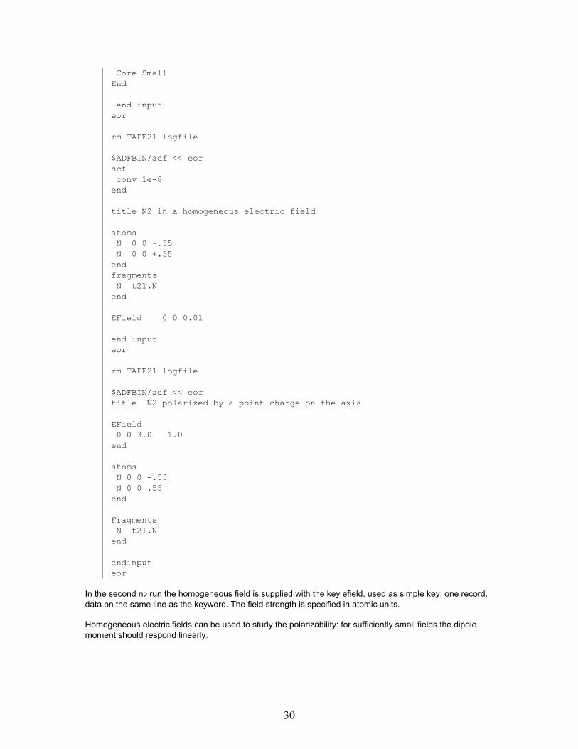
Core SmallEnd
end inputeor
rm TAPE21 logfile
$ADFBIN/adf << eorscfconv 1e-8
end
title N2 in a homogeneous electric field
atomsN 0 0 -.55N 0 0 +.55
endfragmentsN t21.N
end
EField 0 0 0.01
end inputeor
rm TAPE21 logfile
$ADFBIN/adf << eortitle N2 polarized by a point charge on the axis
EField0 0 3.0 1.0
end
atomsN 0 0 -.55N 0 0 .55
end
FragmentsN t21.N
end
endinputeor
In the second n2 run the homogeneous field is supplied with the key efield, used as simple key: one record,data on the same line as the keyword. The field strength is specified in atomic units.
Homogeneous electric fields can be used to study the polarizability: for sufficiently small fields the dipolemoment should respond linearly.
30

For point charges, the third calculation, the block form of the key efield must be used. The program first triesto find data on the same line as the keyword (defining a homogeneous field). If this is absent, a data block isexpected with point-charge specifications: x, y, z and q.
The coordinates are in the same units as in the atoms block (angstrom by default) (but always Cartesian). Qis the charge in elementary units (+1 for a proton).
Point charges can be used for instance to simulate crystal fields (Madelung potential).
Note: the symmetry will be determined automatically by the program as C(lin), rather than D(lin), in the tworuns that involve an electric field: the fields break the symmetry.
For PtCO, a fairly large electric field is applied in combination with a tight SCF convergence criterion.
The BASIS keyword in this example illustrates how different choices can be made for different atoms (in thiscase a frozen core for Pt).
BasisType DZCore NonePt Pt.4d
END
FDE: Frozen Density Embedding
H2O in water: FDE
Sample directory: adf/FDE_H2O_128/
This example demonstrates how to use FDE in combination with a large environment, that is modeled as asuperposition of the densities of isolated molecules. Here, the excitation energies of a water moleculesurrounded by an environment of 127 water molecules. For details, see C.R. Jacob, J. Neugebauer, L.Jensen, L. Visscher, Phys. Chem. Chem. Phys., 2006 8: 2349.
This calculation consists of two steps:
• First a prototype water molecule is calculated.• Next the embedding calculation of water in water is performed.
To reduce the amount of output the next lines are included in the adf calculations:
EPRINTSFO NOEIG NOOVL NOORBPOPSCF NOPOP
ENDNOPRINT BAS FUNCTIONS
First, a prototype water molecule is calculated. The density of this isolated water molecules will afterwardsbe used to model the environment. Since this molecule will be used as a frozen fragment that is rotated andtranslated, the option NOSYMFIT has to be included.
$ADFBIN/adf << eorTitle Input generated by modco
31

UNITSlength bohrangle degree
END
XCLDAEND
SYMMETRY NOSYM
GEOMETRYsp
END
SCFiterations 50converge 1.0e-6 1.0e-6mixing 0.2lshift 0.0diis n=10 ok=0.5 cyc=5 cx=5.0 cxx=10.0
ENDINTEGRATION 5.0 5.0
FRAGMENTSO t21.DZP.OH t21.DZP.H
END
ATOMSO -11.38048700000000 -11.81055300000000
-4.51522600000000H -13.10476265095705 -11.83766918322447
-3.96954531282721H -10.51089289290947 -12.85330720999229
-3.32020577897331END
ENDINPUTeor
mv TAPE21 t21.mol_1
Afterwards, the FDE calculation is performed. In this FDE calculation, there is one nonfrozen water moleculeand the previously prepared water molecule is included as a frozen fragment that is duplicated 127 times.For this frozen fragment, the more efficient fitted density is used.
$ADFBIN/adf << eorTitle Input generated by modco
UNITSlength bohrangle degree
END
XCMODEL SAOP
32

END
SYMMETRY NOSYM
SCFiterations 50converge 1.0e-6 1.0e-6mixing 0.2lshift 0.0diis n=10 ok=0.5 cyc=5 cx=5.0 cxx=10.0
END
EXCITATIONONLYSINGLOWEST 5
END
INTEGRATION 4.0 4.0
FRAGMENTSO t21.DZP.OH t21.DZP.Hfrag1 t21.mol_1 type=fde &
fdedenstype SCFfittedSubEnd
END
ATOMSO 0.00000000000000 0.00000000000000 0.00000000000000H -1.43014300000000 0.00000000000000 1.10739300000000H 1.43014300000000 0.00000000000000 1.10739300000000O -11.38048700000000 -11.81055300000000 -4.51522600000000 f=frag1/1H -13.10476265095705 -11.83766918322447 -3.96954531282721 f=frag1/1H -10.51089289290947 -12.85330720999229 -3.32020577897331 f=frag1/1O -1.11635000000000 9.11918600000000 -3.23094800000000 f=frag1/2H -2.82271357869859 9.71703285239153 -3.18063201242303 f=frag1/2H -0.12378551814273 10.53819303003839 -2.70860866559857 f=frag1/2
...O 5.96480100000000 4.51370300000000 3.70332800000000 f=frag1/127H 5.24291272273548 3.06620845434369 2.89384293177905 f=frag1/127H 4.73614594944492 5.00201400735317 4.93765482424434 f=frag1/127
END
FDEPW91K
END
ENDINPUTeor
HeCO2: FDE freeze-and-thaw
Sample directory: adf/FDE_HeCO2_freezeandthaw/
33

This example demonstrates how a freeze-and-thaw FDE calculation can be performed. As test system, aHe-CO2van der Waals complex is used. It will further be shown how different exchange-correlation potentialcan be used for different subsystems, and how different basis set expansions can be employed. For details,see C.R. Jacob, T.A. Wesolowski, L. Visscher, J. Chem. Phys. 123 (2005), 174104. It should be stressedthat the basis set and integration grid used in this example are too small to obtain good results.
Summary:
• PW91 everywhere• SAOP for He; PW91 for CO2• FDE(s) calculation with PW91 everywhere
PW91 everywhere
In the first part, the PW91 functional will be used for both the He and the CO2 subsystems. In this part, theFDE(m) basis set expansion is used, i.e., basis functions of the frozen subsystem are not included in thecalculation of the nonfrozen subsystem.
First, the CO2 molecule is prepared. In this calculation, the C2v symmetry of the final complex is used, andthe NOSYMFIT option has to be included because this molecule will be rotated as a frozen fragment.
$ADFBIN/adf << eorTitle TEST 1 -- Preparation of frozen CO2
UnitsLength Bohr
end
AtomsC 0.000000 0.000000 0.000000O -2.192000 0.000000 0.000000O 2.192000 0.000000 0.000000end
Symmetry C(2V)NOSYMFIT
FragmentsC t21.CO t21.O
End
integration 5.0
xcGGA pw91
end
End Inputeor
mv TAPE21 t21.co2.0
Afterwards, the FDE calculation is performed. In this calculation, the He atom is the nonfrozen system, andthe previously prepared CO2 molecule is used as frozen fragment. For this frozen fragment the RELAX
34

option is specified, so that the density of this fragment is updated in freeze-and-thaw iteration (a maximumnumber of three iteration is specified).
$ADFBIN/adf << eorTitle TEST 1 -- Embedding calulation: He + frozen CO2 density --freeze-and-thaw
UnitsLength Bohr
end
AtomsHe 0.000000 0.000000 6.019000 f=HeC 0.000000 0.000000 0.000000 f=co2O -2.192000 0.000000 0.000000 f=co2O 2.192000 0.000000 0.000000 f=co2
end
FragmentsHe t21.Heco2 t21.co2.0 type=fde &
fdeoptions RELAXSubEnd
End
NOSYMFIT
integration 5.0
xcGGA pw91
end
FDEPW91KFULLGRIDRELAXCYCLES 3
end
End Inputeor
SAOP for He; PW91 for CO2
In this second part, the above example is modified such that PW91 is employed for the CO2 subsystem,while the SAOP potential is used for He. This can be achieved by choosing SAOP in the XC key (this setsthe functional that will be used for the nonfrozen subsystem). Additionally, for the frozen fragment the XCoption is used to chose the PW91 functional for relaxing this fragment. Furthermore, the PW91 functional ischosen for the nonadditive exchange-correlation functional that is used in the embedding potential with theGGAPOTXFD and GGAPOTCFD options in the FDE key.
$ADFBIN/adf << eorTitle TEST 2 -- Embedding calulation: He + frozen CO2 density --freeze-and-thaw
Units
35

Length Bohrend
AtomsHe 0.000000 0.000000 6.019000 f=HeC 0.000000 0.000000 0.000000 f=co2O -2.192000 0.000000 0.000000 f=co2O 2.192000 0.000000 0.000000 f=co2
end
FragmentsHe t21.Heco2 t21.co2.0 type=fde &
fdeoptions RELAXXC GGA PW91
SubEndEnd
NOSYMFIT
integration 5.0
xcMODEL SAOP
end
FDEPW91KFULLGRIDGGAPOTXFD PW91xGGAPOTCFD PW91cRELAXCYCLES 3
end
End Inputeor
FDE(s) calculation with PW91 everywhere
In this third part, the PW91 functional is applied for both subsystems again, but in contrast to part 1, now theFDE(s) basis set expansion is used, i.e., the basis functions of the frozen subsystem are included in thecalculation of the nonfrozen subsystem. This can be achieved by employing the USEBASIS option. Thisoption can be combined with the RELAX option.
$ADFBIN/adf << eorTitle TEST 3 -- Embedding calulation: He + frozen CO2 density --freeze-and-thaw
UnitsLength Bohr
end
AtomsHe 0.000000 0.000000 6.019000 f=HeC 0.000000 0.000000 0.000000 f=co2O -2.192000 0.000000 0.000000 f=co2
36

O 2.192000 0.000000 0.000000 f=co2end
FragmentsHe t21.Heco2 t21.co2.0 type=fde &
fdeoptions RELAX USEBASISSubEnd
End
NOSYMFIT
integration 5.0
xcGGA pw91
end
FDEPW91KFULLGRIDRELAXCYCLES 3
end
End Inputeoreor
The example continues with the same calculation where partly the SAOP potential is used.
NH3-H2O: FDE energy
Sample directory: adf/FDE_Energy_NH3-H2O/
This is example for a calculation of FDE interaction energies in ADF in case of closed shell fragments.
It performs single point runs for H2O and NH3 with LDA/DZ (all-electron) and uses these fragments in:
• an FDE energy embedding calculation calculation in which the energy of water in presence of afrozen ammonia is computed This requires a supermolecular integration grid
• a fully variational FDE energy calculation (with freeze-and-thaw)
Integration accuracy is 6.0 which should give total energies for the fragments accurate at least up to 10**(-4)atomic units.
$ADFBIN/adf << EOFTitle H2O LDA/DZ single pointATOMS
O 1.45838 0.10183 0.00276H 0.48989 -0.04206 0.00012H 1.84938 -0.78409 -0.00279
ENDSYMMETRY tol=1e-2BASIS
Type DZ
37

Core NoneENDXC
LDAENDINTEGRATIONaccint 6.0
ENDNOSYMFIT
EOFrm logfilemv TAPE21 t21.waterEOF
In a similar way the N3 fragment is calculated. Next the FDE calculation is performed. The subkey ENERGYof the key FDE is used, such that the total FDE energy and FDE interaction energy is calculated. First anFDE energy embedding calculation calculation in which the energy of water in presence of a frozenammonia is computed. This requires a supermolecular integration grid.
$ADFBIN/adf << EOFTitle NH3-H2O LDA/Thomas-Fermi/DZ FDE single point with interaction energyATOMS
O 1.45838 0.10183 0.00276 f=frag1H 0.48989 -0.04206 0.00012 f=frag1H 1.84938 -0.78409 -0.00279 f=frag1N -1.51248 -0.03714 -0.00081 f=frag2H -1.71021 0.95994 -0.11003 f=frag2H -1.96356 -0.53831 -0.76844 f=frag2H -1.92899 -0.35123 0.87792 f=frag2
ENDSYMMETRY tol=1e-2FRAGMENTSfrag1 t21.waterfrag2 t21.ammonia type=FDE
ENDXC
LDAENDINTEGRATIONaccint 6.0
ENDEXACTDENSITYFDE
THOMASFERMIFULLGRIDENERGY
ENDEOF
Next a fully variational FDE energy calculation (with freeze-and-thaw) is performed.
$ADFBIN/adf << EOFTitle NH3-H2O LDA/Thomas-Fermi/DZ FDE single point with interaction energyATOMS
O 1.45838 0.10183 0.00276 f=frag1H 0.48989 -0.04206 0.00012 f=frag1H 1.84938 -0.78409 -0.00279 f=frag1N -1.51248 -0.03714 -0.00081 f=frag2
38

H -1.71021 0.95994 -0.11003 f=frag2H -1.96356 -0.53831 -0.76844 f=frag2H -1.92899 -0.35123 0.87792 f=frag2
ENDSYMMETRY tol=1e-2FRAGMENTSfrag1 t21.waterfrag2 t21.ammonia type=FDE &
fdeoptions RELAXSubEnd
ENDXC
LDAENDINTEGRATIONaccint 6.0
ENDEXACTDENSITYSAVE TAPE21FDE
THOMASFERMIRELAXCYCLES 3ENERGY
ENDEOF
Ne-H2O: FDE energy, unrestricted fragments
Sample directory: adf/FDE_Energy_H2O-Ne_unrestricted/
This is example for a calculation of FDE interaction energies in ADF for an open-shell frozen fragment.
It performs single point runs for H2O and Ne, the latter unrestricted with LDA/DZ (all-electron) and usesthese fragments in an FDE energy embedding calculation in which the energy of water in presence of afrozen (open-shell) neon atom is computed. This is a bit of an artificial example but it serves its purpose.
No freeze-thaw is done, this is at present not possible with unrestricted (open shell) fragments, but has to bedone manually.
Integration accuracy is 6.0 which should give total energies for the fragments accurate at least up to 10**(-4)atomic units.
This test has been checked to yield the same energy as a run with a closed- shell (restricted) Ne atom (justcomment UNRESTRICTED in the input below). First the Ne and H2O fragments are calculated.
$ADFBIN/adf << EOFTitle Ne LDA/DZ single point, unrestrictedATOMS
Ne -1.51248 -0.03714 -0.00081ENDUNRESTRICTEDBASIS
Type DZCore None
END
39

INTEGRATIONaccint 6.0
ENDSCF
iterations 100converge 1.0e-06 1.0e-06
ENDEXACTDENSITYNOSYMFIT
EOF
rm logfilemv TAPE21 t21.neEOF
In a similar way the H2O fragment is calculated. Next the FDE calculation is performed. The subkeyENERGY of the key FDE is used, such that the total FDE energy and FDE interaction energy is calculated.
$ADFBIN/adf << EOFTitle Ne-H2O LDA/Thomas-Fermi/DZ FDE single point with interaction energy
ATOMSO 1.45838 0.10183 0.00276 f=frag1H 0.48989 -0.04206 0.00012 f=frag1H 1.84938 -0.78409 -0.00279 f=frag1Ne -1.51248 -0.03714 -0.00081 f=frag2
END
SYMMETRY tol=1e-2
FRAGMENTSfrag1 t21.waterfrag2 t21.ne type=FDE
END
INTEGRATIONaccint 6.0
END
SCFiterations 100converge 1.0e-06 1.0e-06
END
EXACTDENSITY
FDETHOMASFERMIFULLGRIDENERGY
ENDEOF
H2O-Li(+): FDE geometry optimization
40
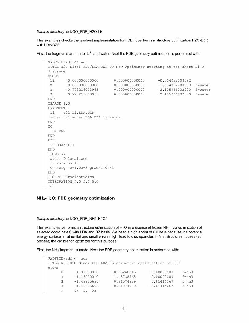
Sample directory: adf/GO_FDE_H2O-Li/
This examples checks the gradient implementation for FDE. It performs a structure optimization H2O-Li(+)with LDA/DZP.
First, the fragments are made, Li+, and water. Next the FDE geometry optimization is performed with:
$ADFBIN/adf << eorTITLE H2O-Li(+) FDE/LDA/DZP GO New Optimizer starting at too short Li-OdistanceATOMSLi 0.000000000000 0.000000000000 -0.054032208082O 0.000000000000 0.000000000000 -1.534032208080 f=waterH -0.778216093965 0.000000000000 -2.135966332900 f=waterH 0.778216093965 0.000000000000 -2.135966332900 f=water
ENDCHARGE 1.0FRAGMENTSLi t21.Li.LDA.DZPwater t21.water.LDA.DZP type=fde
ENDXCLDA VWN
ENDFDEThomasFermi
ENDGEOMETRYOptim Delocalizediterations 15Converge e=1.0e-3 grad=1.0e-3
ENDGEOSTEP GradientTermsINTEGRATION 5.0 5.0 5.0eor
NH3-H2O: FDE geometry optimization
Sample directory: adf/GO_FDE_NH3-H2O/
This examples performs a structure optimization of H2O in presence of frozen NH3 (via optimization ofselected coordinates) with LDA and DZ basis. We need a high accint of 6.0 here because the potentialenergy surface is rather flat and small errors might lead to discrepancies in final structures. It uses (atpresent) the old branch optimizer for this purpose.
First, the NH3 fragment is made. Next the FDE geometry optimization is performed with:
$ADFBIN/adf << eorTITLE NH3-H2O dimer FDE LDA DZ structure optimization of H2OATOMS
N -1.01393958 -0.15260815 0.00000000 f=nh3H -1.16290010 -1.15738765 0.00000000 f=nh3H -1.49925696 0.21074929 0.81414267 f=nh3H -1.49925696 0.21074929 -0.81414267 f=nh3O Ox Oy Oz
41

H H1x H1y H1zH H2x H2y H2z
ENDGEOVAROx 2.25288687Oy -0.00423586Oz 0.00000000H1x 1.28270504H1y 0.05211069H1z 0.00000000H2x 2.54788803H2y 0.90516678H2z 0.00000000
ENDFRAGMENTSO t21.O_LDA_DZH t21.H_LDA_DZnh3 t21.NH3_LDA_DZ type=fde
ENDFDETHOMASFERMI
ENDXCLDA VWN
ENDGEOMETRYBranch OldOptim SelectedIterations 100 ! (default is 30)
ENDINTEGRATION 6.0 6.0 6.0eor
Acetonitrile in water: FDE NMR shielding
Sample directory: adf/FDE_NMR_relax/
This examples demonstrates both the calculation of NMR shieldings using FDE, and how the approximateenvironment density can be improved by partial relaxation of individual solvent molecules. The test system isa cluster of acetonitrile and 12 solvent water molecules, of which for two the densities are relaxed, while forthe remaining 10 the frozen density of the isolated water is used. For details, see Refs.C. R. Jacob, J. Neugebauer, and L. Visscher, A flexible implementation of frozendensity embedding for usein multilevel simulation, submitted, 2007.R. E. Bulo, Ch. R. Jacob, and L. Visscher, NMR Solvent Shifts of Acetonitrile from Frozen-DensityEmbedding Calculation, to be submitted, 2007
First, the isolated solvent water molecule is prepared. Again, because this will be rotated and translatedafterwards, the option NOSYMFIT has to be included.
$ADFBIN/adf << eor
UNITSLength AngstromAngle Degree
42

END
ATOMSO -1.46800 2.60500 1.37700H -0.95200 3.29800 0.96500H -1.16100 1.79900 0.96100
END
FRAGMENTSH t21.H.DZPO t21.O.DZP
END
XCLDA
END
INTEGRATIONaccint 4.0
END
end inputeor
mv TAPE21 t21.h2o
Afterwards, the FDE calculation is performed. In addition to the nonfrozen acetonitrile molecule, threedifferent fragments are used for the solvent water molecules. The first two fragments frag1 and frag2 arerelaxed (in up to two freeze-and-thaw cycles), while the third fragment is used for the remaining 10 solventmolecules. Since a calculation of the shielding is performed afterwards, the option has to be included.
$ADFBIN/adf << eorTitle Input generated by PyADF
UNITSLength AngstromAngle Degree
END
ATOMSC 0.83000 0.66100 -0.44400N 0.00000 0.00000 0.00000C 1.87800 1.55900 -0.81900H 1.78500 2.40300 -0.13500H 1.76200 1.94900 -1.83000H 2.82900 1.12200 -0.51300O -1.46800 2.60500 1.37700 f=frag1/1H -0.95200 3.29800 0.96500 f=frag1/1H -1.16100 1.79900 0.96100 f=frag1/1O 2.40400 -2.51000 -0.36200 f=frag2/1H 2.70000 -3.41900 -0.40900 f=frag2/1H 1.77500 -2.50000 0.35900 f=frag2/1
...O -3.44400 2.36700 3.13700 f=frag3/10H -2.70200 2.29200 2.53700 f=frag3/10H -3.47300 3.29500 3.36800 f=frag3/10
END
43

FRAGMENTSH t21.H.DZPC t21.C.DZPN t21.N.DZPfrag1 t21.h2o type=FDE &
fdeoptions RELAXRELAXCYCLES 2
SubEndfrag2 t21.h2o type=FDE &
fdeoptions RELAXRELAXCYCLES 2
SubEndfrag3 t21.h2o type=FDE &
FDEDENSTYPE SCFexactSubEnd
END
XCGGA BP86
END
INTEGRATIONaccint 4.0
END
SAVE TAPE10
FDEPW91k
END
End Inputeor
Finally, the calculation of the NMR shielding of the nitrogen atom is performed using the NMR program.
$ADFBIN/adf << eorNMRout tens isonuc 3
ENDeor
Subsystem TDDFT, coupled FDE excitation energies
Sample directory: adf/SUBEXCI_dimer/
This is example for coupled FDE calculation of excitatione energies. The subsystem TDDFT code couplesthe monomer excitations to obtain the excited states of the total system (often denoted as coupled frozendensity embedding, FDEc).
44

First the isolated fragments are calculated, the TAPe21's of these fragments are t21.iso.rho1 andt21.iso.rho2. Next uncoupled FDE excitation energies are calculated in which one fragment is frozen and theother active. The key ALLOW PARTIALSUPERFRAGS is necessary to be able to use subsysteminformation for only one subsystem from a TAPE21 file of a previous FDE calculation.
$ADFBIN/adf << eorTitle Fragment no. 1; relaxedSYMMETRY NOSYMXC
GGA BECKE88 PERDEW86ENDEXCITATION
ONLYSINGLOWEST 20CDSPECTRUMANALYTICVELOCITY
ENDALLOW PARTIALSUPERFRAGSFRAGMENTS
rho1 t21.iso.rho1 subfrag=activerho2 t21.iso.rho2 subfrag=active type=fde
ENDATOMS
1 C 1.05754858422573 -1.70701086799077 -3.50 f=rho12 O 2.28164544472573 -1.70701086799077 -3.50 f=rho13 C 0.20221626882573 -0.49944933059077 -3.50 f=rho14 H 0.49106545372573 -2.67285236319077 -3.50 f=rho15 C -1.19491351307427 -0.64892031589077 -3.50 f=rho16 C 0.76942690052573 0.78743686120923 -3.50 f=rho17 C -2.02186702237427 0.47538393990923 -3.50 f=rho18 H -1.62606655117427 -1.65281003349077 -3.50 f=rho19 C -0.05719256647427 1.90851291410923 -3.50 f=rho1
10 H 1.85606600152573 0.87752625020923 -3.50 f=rho111 C -1.45186603427427 1.75322106580923 -3.50 f=rho112 H -3.10608163477427 0.35931991730923 -3.50 f=rho113 H 0.37787441672573 2.90894982040923 -3.50 f=rho114 H -2.09570824397427 2.63406412680923 -3.50 f=rho115 C 2.00708906832899 0.06235850568037 3.50 f=rho216 O 2.61913749857899 1.12245748356614 3.50 f=rho217 C 0.53364394260760 -0.07460023943380 3.50 f=rho218 H 2.56029077395134 -0.91115102374797 3.50 f=rho219 C -0.03547527794391 -1.35928561559301 3.50 f=rho220 C -0.29722687542061 1.06006167281502 3.50 f=rho221 C -1.42262807969967 -1.51329623449550 3.50 f=rho222 H 0.61834220104568 -2.23461995830645 3.50 f=rho223 C -1.68141695030640 0.90472624158027 3.50 f=rho224 H 0.16807297559397 2.04616343352651 3.50 f=rho225 C -2.24426699857796 -0.38074233566867 3.50 f=rho226 H -1.86422099386266 -2.51028564328820 3.50 f=rho227 H -2.33028723444571 1.78172375452933 3.50 f=rho228 H -3.32902057100121 -0.49790451479758 3.50 f=rho2
ENDFDE
PW91KENDEND INPUT
45

eormv TAPE21 t21.emb.rho1
$ADFBIN/adf << eorTitle Fragment no. 2; relaxedSYMMETRY NOSYMXC
GGA BECKE88 PERDEW86ENDEXCITATION
ONLYSINGLOWEST 20CDSPECTRUMANALYTICVELOCITY
ENDALLOW PARTIALSUPERFRAGSFRAGMENTS
rho1 t21.emb.rho1 subfrag=active type=fderho2 t21.iso.rho2 subfrag=active
ENDATOMS
1 C 1.05754858422573 -1.70701086799077 -3.50 f=rho12 O 2.28164544472573 -1.70701086799077 -3.50 f=rho13 C 0.20221626882573 -0.49944933059077 -3.50 f=rho14 H 0.49106545372573 -2.67285236319077 -3.50 f=rho15 C -1.19491351307427 -0.64892031589077 -3.50 f=rho16 C 0.76942690052573 0.78743686120923 -3.50 f=rho17 C -2.02186702237427 0.47538393990923 -3.50 f=rho18 H -1.62606655117427 -1.65281003349077 -3.50 f=rho19 C -0.05719256647427 1.90851291410923 -3.50 f=rho1
10 H 1.85606600152573 0.87752625020923 -3.50 f=rho111 C -1.45186603427427 1.75322106580923 -3.50 f=rho112 H -3.10608163477427 0.35931991730923 -3.50 f=rho113 H 0.37787441672573 2.90894982040923 -3.50 f=rho114 H -2.09570824397427 2.63406412680923 -3.50 f=rho115 C 2.00708906832899 0.06235850568037 3.50 f=rho216 O 2.61913749857899 1.12245748356614 3.50 f=rho217 C 0.53364394260760 -0.07460023943380 3.50 f=rho218 H 2.56029077395134 -0.91115102374797 3.50 f=rho219 C -0.03547527794391 -1.35928561559301 3.50 f=rho220 C -0.29722687542061 1.06006167281502 3.50 f=rho221 C -1.42262807969967 -1.51329623449550 3.50 f=rho222 H 0.61834220104568 -2.23461995830645 3.50 f=rho223 C -1.68141695030640 0.90472624158027 3.50 f=rho224 H 0.16807297559397 2.04616343352651 3.50 f=rho225 C -2.24426699857796 -0.38074233566867 3.50 f=rho226 H -1.86422099386266 -2.51028564328820 3.50 f=rho227 H -2.33028723444571 1.78172375452933 3.50 f=rho228 H -3.32902057100121 -0.49790451479758 3.50 f=rho2
ENDFDE
PW91KENDEND INPUTeor
46

mv TAPE21 t21.emb.rho2
Finally a calculation in which the excitation energies may couple, using the SUBEXCI block keyword.
$ADFBIN/adf << eorTitle COUPLED SUBSYSTEM EXCITATIONSSYMMETRY NOSYMXC
GGA BECKE88 PERDEW86ENDDIFFUSEALLOW PARTIALSUPERFRAGSFRAGMENTS
rho1 t21.emb.rho1 subfrag=activerho2 t21.emb.rho2 subfrag=active type=fde
ENDATOMS
1 C 1.05754858422573 -1.70701086799077 -3.50 f=rho12 O 2.28164544472573 -1.70701086799077 -3.50 f=rho13 C 0.20221626882573 -0.49944933059077 -3.50 f=rho14 H 0.49106545372573 -2.67285236319077 -3.50 f=rho15 C -1.19491351307427 -0.64892031589077 -3.50 f=rho16 C 0.76942690052573 0.78743686120923 -3.50 f=rho17 C -2.02186702237427 0.47538393990923 -3.50 f=rho18 H -1.62606655117427 -1.65281003349077 -3.50 f=rho19 C -0.05719256647427 1.90851291410923 -3.50 f=rho1
10 H 1.85606600152573 0.87752625020923 -3.50 f=rho111 C -1.45186603427427 1.75322106580923 -3.50 f=rho112 H -3.10608163477427 0.35931991730923 -3.50 f=rho113 H 0.37787441672573 2.90894982040923 -3.50 f=rho114 H -2.09570824397427 2.63406412680923 -3.50 f=rho115 C 2.00708906832899 0.06235850568037 3.50 f=rho216 O 2.61913749857899 1.12245748356614 3.50 f=rho217 C 0.53364394260760 -0.07460023943380 3.50 f=rho218 H 2.56029077395134 -0.91115102374797 3.50 f=rho219 C -0.03547527794391 -1.35928561559301 3.50 f=rho220 C -0.29722687542061 1.06006167281502 3.50 f=rho221 C -1.42262807969967 -1.51329623449550 3.50 f=rho222 H 0.61834220104568 -2.23461995830645 3.50 f=rho223 C -1.68141695030640 0.90472624158027 3.50 f=rho224 H 0.16807297559397 2.04616343352651 3.50 f=rho225 C -2.24426699857796 -0.38074233566867 3.50 f=rho226 H -1.86422099386266 -2.51028564328820 3.50 f=rho227 H -2.33028723444571 1.78172375452933 3.50 f=rho228 H -3.32902057100121 -0.49790451479758 3.50 f=rho2
ENDFDE
PW91KENDSUBEXCI
CTHRES 10000.00SFTHRES 0.00010000COUPLBLOCK
ENDEND INPUTeor
47

QM/MM calculations
pdb2adf: transforms a PDB file in a QM/MM adf-input file
Sample directory: adf/pdb2adf/
This example shows how to use the utiliy pdb2adf, which creates an ADF input file from a PDB file, for asubsequent QM/MM calculation using ADF. See also the Utilities document for more examples.
First create the PDB file that can be used in this example.
cat << eor > chymotrypsin.pdbHEADER COMPLEX (SERINE PROTEASE/INHIBITOR) 12-MAR-97 1AFQTITLE CRYSTAL STRUCTURE OF BOVINE GAMMA-CHYMOTRYPSIN COMPLEXEDTITLE 2 WITH A SYNTHETIC INHIBITORREMARKREMARK Adaptation of original PDB file by M. Swart, March 2005REMARK only coordinates of GAMMA-CHYMOTRYPSIN are kept;REMARK rest has been deleted.REMARKATOM 1 N CYS A 1 13.717 20.021 22.754 1.00 13.46 PROA NATOM 2 CA CYS A 1 14.211 18.932 23.617 1.00 13.34 PROA CATOM 3 C CYS A 1 13.597 19.033 25.005 1.00 13.34 PROA C...ATOM 68 CD2 LEU A 10 9.768 11.681 39.555 1.00 27.46 PROA CATOM 69 OXT LEU A 10 6.329 11.066 42.743 1.00 27.55 PROA OTER 70 LEU A 10ENDeor
Then run the pdf2adf program to create ADF inputfile
$ADFBIN/pdb2adf << eor
chymotrypsin.pdb
4 5c
Y1117.5eor
The program works interactively. The input described here are answers to the questions that were askedinteractively. In cases where the user agrees with the suggestion given by the program, the user can pressthe Enter key, which is shown here with an empty line.
The questions asked can be found in the output file, and are repeated here. The Enter key or empty line isindicated here with Enter.
Do you want a logfile to be written (Y/n) ?
Enter
Please give name of PDB-file
48

chymotrypsin.pdb
Found the following terminal amino acid residues : (C-term) 10(N-term) 1Do you want to use these as terminal residues (Y/n) ?
Enter
Multiple AMBER options for CYS :0 Decide every time differently1 CYS Cysteine (SH)2 CYM Deprotonated Cysteine (S-)3 CYX Cystine (S-S bridge)
Suggested option: 0
Enter
Multiple AMBER options for CYS 1 ( 1) :1 CYS Cysteine (SH)2 CYX Cystine (S-S bridge)Connections and Nearest Atoms for SG CYS 1 SG ( P2A # 8 PDB# 6 )
Dist P2A Nr PDB Nr Label Near Dist P2A Nr PDB Nr Label1 1.83 5 5 CB CYS 1 CB 1 5.58 19 0 H1 GLY 2
2 6.06 36 0 HC VAL 33 6.09 26 0 H VAL 34 6.47 25 11 N VAL 3 N5 7.15 35 17 CT VAL 3 CG2
Suggestion: 1
Enter
Option Molecule Option Molecule Option Molecule Option Molecule Option Molecule1: CYS 1 4: PRO 4 7: GLN 7 10: LEU 102: GLY 2 5: ALA 5 8: PRO 83: VAL 3 6: ILE 6 9: VAL 9
Give option number of molecules to be put in QM region (or 'c' to continue):Note: by specifying a negative number a molecule is removed from the QM region
4 5
Give option number of molecules to be put in QM region (or 'c' to continue):Note: by specifying a negative number a molecule is removed from the QM region
c
Make a choice for the QM/MM treatment of PRO 40: Put completely in QM region1: Cut off at C-alpha (put NH in QM region, CO in MM region)2: Cut off at C-alpha (put NH in MM region, CO in QM region)3: Cut off at C-alpha (put NH and CO in MM region)4: Cut off at C-alpha (put NH and CO in QM region, sidechain in MM region)5: Put only part of sidechain in QM region
Suggestion: 2...Give choice:
Enter
Make a choice for the QM/MM treatment of ALA 50: Put completely in QM region1: Cut off at C-alpha (put NH in QM region, CO in MM region)
49

2: Cut off at C-alpha (put NH in MM region, CO in QM region)3: Cut off at C-alpha (put NH and CO in MM region)4: Cut off at C-alpha (put NH and CO in QM region, sidechain in MM region)5: Put only part of sidechain in QM region
Suggestion: 1Give choice:
Enter
Do you want to add solvent to your system (Y/n) ?
Y
Solvent (box) available:1: HOH HOH Water molecule2: MOH MOH Methanol molecule3: CHL CHL Chloroform molecule
1
Make a choice:
1
Give boxsize (def.: 16.71 Angs)
17.5
QMMM_Butane: Basic QMMM Illustration
Sample directory: adf/QMMM_Butane/
This example is a simple illustration of the QMMM functionality: half of the butane molecule is treatedquantum-mechanically, the other half by molecular mechanics.
$ADFBIN/adf << eorTitle BUTANE in Z-matrix input
(Omitted in this printout: the usual specifications of fragments, symmetry, integration accuracy, -)
QMMMFORCEFIELD_FILE $ADFRESOURCES/ForceFields/amber95.ffRESTART_FILE mm.restartOUTPUT_LEVEL=2WARNING_LEVEL=2ELSTAT_COUPLING_MODEL=0
LINKS1 - 4 1.38000 H
SUBEND
MM_CONNECTION_TABLE1 CT QM 2 3 4 52 HC QM 1
50

3 HC QM 14 CT LI 1 9 13 145 CT QM 1 6 7 86 HC QM 57 HC QM 58 HC QM 59 CT MM 4 10 11 12
10 HC MM 911 HC MM 912 HC MM 913 HC MM 414 HC MM 4
SUBEND
End
Atoms InternalC 0 0 0 0 0 0H 1 0 0 B1 0 0H 1 2 0 B2 A1 0C 1 2 3 B3 A2 D1C 1 2 3 B4 A3 D2H 5 1 2 B5 A4 D3H 5 1 6 B6 A5 D4H 5 1 6 B7 A6 D5C 4 1 2 B8 A7 D6H 9 4 1 B9 A8 D7H 9 4 10 B10 A9 D8H 9 4 10 B11 A10 D9H 4 1 9 B12 A11 D10H 4 1 9 B13 A12 D11
End
GeoVar....
In the QMMM key block, the MM connection table identifies the atoms as belonging to either the QM(quantum mechanics) part, or the MM (molecular mechanics) part, or to the set of LI (link) atoms, whichdefine the connection between the QM and the MM regions. Order and numbering are one-to-one with thelist under the Atoms key.
The Link atom, part of the MM section of the system, is associated with a capping atom, in the QM part ofthe system. The Links subkey block specifies for each LI atom defined under the MM_Connection_Tablesubkey block the chemical type of the replacing capping atom (here: H). On the same line we find the ratioof the QM atom LI atom distance to the QM atom capping atom distance (here: 1.38), and the numbers (1and 4) of the involved QM atom and LI atom.
The other subkeys in the QM key block are simple subkeys. The specify the file with the force fieldparameters to be used in the MM subsystem, the (restart) file to write MM data to, print and warning levelsand a code for the electrostatic coupling model to use. See the QMMM manual for a detailed discussion ofall options.
The calculation is a simple geometry optimization (the Geometry key is not displayed here, but is containedin the full input). This consists of a repeated two-step process. At the first step, the MM system is keptfrozen, the SCF equations are solved for the QM system, where potentials resulting from the MM system areincluded, and gradients on the QM atoms are computed from the SCF solution. At the second step, the QMsystem's geometry is updated and then kept frozen while the MM system's geometry is optimized
51

(converged) for that particular QM configuration. And so on, until the whole combined system is self-consistently converged.
QMMM_CYT
Sample directory: adf/QMMM_CYT/
See the QMMM manual , where this case is used as a 'walk through' for the QMMM feature.
It is a more or less straightforward application of QMMM to geometry optimization (Cytocine). In the Atomsblock all atoms are listed (QM as well as MM). All QMMM aspects, such as which atoms belong to the QMcore and which are to be treated by the approximate MM method, are found in the QMMM key block, and itsvarious subkey blocks. The remainder of the input file is not different from what it would be in a non-QMMMrun.
The standard amber95 force field is used, which is located in the database of the ADF distribution.
$ADFBIN/adf << eorTitle CYT amber95 - Cartesian Geometry Optimization
FragmentsC t21.CH t21.H
End
Charge 0 0
Atoms Cartesian1 C 1.94807 3.58290 -0.581622 C 1.94191 3.61595 1.094483 H 1.69949 4.49893 -1.052734 H 2.99455 3.17964 -0.863045 C 0.94659 2.40054 -0.923646 N -1.74397 -3.46417 0.311787 C -1.00720 -2.20758 0.335368 C -1.66928 -1.00652 0.310019 C -0.92847 0.25653 0.34895
10 N 0.43971 0.26735 0.3823211 N 0.36409 -2.20477 0.2899212 C 1.09714 -0.95413 0.2246913 H -2.89781 -3.50815 0.3174614 H -1.21484 -4.49217 0.3172115 H -2.80940 -0.93497 0.3055016 H -1.55324 1.21497 0.3388517 C 1.23309 1.44017 0.3099418 O 2.58277 -1.01636 0.2391419 H 2.37276 1.25557 0.2998420 O 1.02358 2.43085 1.5088021 H 1.17136 1.95097 -1.8736722 H -0.10600 2.77333 -0.8034823 H 1.62170 4.54039 1.5139224 H 2.99608 3.28749 1.41345
End
52

QMMMFORCEFIELD_FILE $ADFRESOURCES/ForceFields/amber95.ffRESTART_FILE mm.restartOUTPUT_LEVEL=1WARNING_LEVEL=2ELSTAT_COUPLING_MODEL=1
LINK_BONDS1 - 5 1.38000 H1 - 2 1.38030 H
SUBEND
MM_CONNECTION_TABLE1 CT QM 2 3 4 52 CT LI 1 20 23 243 HC QM 14 HC QM 15 CT LI 1 17 21 226 N2 MM 7 13 147 CA MM 6 8 118 CM MM 7 9 159 CM MM 8 10 16
10 N* MM 9 12 1711 NC MM 7 1212 C MM 10 11 1813 H MM 614 H MM 615 HA MM 816 H4 MM 917 CT MM 5 10 19 2018 O MM 1219 H2 MM 1720 OS MM 2 1721 HC MM 522 HC MM 523 H1 MM 224 H1 MM 2
SUBEND
CHARGES1 0.0 CT2 0.0 CT3 0.0 HC4 0.0 HC5 0.0 CT6 -0.9530 N27 0.8185 CA8 -0.5215 CM9 0.0053 CM
10 -0.0484 N*11 -0.7584 NC12 0.7538 C13 0.4234 H14 0.4234 H15 0.1928 HA16 0.1958 H417 0.0066 CT
53

18 -0.6252 O19 0.2902 H220 -0.2033 OS21 0.0000 HC22 0.0000 HC23 0.0000 H124 0.0000 H1
SUBEND
END
GeometryIterations 20Converge E=1.0E-3 Grad=0.0005Step Rad=0.3 Angle=5.0
End
XCLDA VWNGGA PostSCF Becke Perdew
End
Integration 3.0
SCFIterations 60Converge 1.0E-06 1.0E-6Mixing 0.20DIIS N=10 OK=0.500 CX=5.00 CXX=25.00 BFAC=0.00
End
End Inputeor
QMMM_Surface: Ziegler-Natta catalysis
Sample directory: adf/QMMM_Surface/
This is an example of a Ziegler-Natta type catalytic system: a TiCl complex embedded in a MgCl surfacewith two organic substrates also attached to the surface. To make the computation faster, the QMMMapproach is applied. The QM part includes only the active site and a piece of the MgCl surface.
The computation is formally a geometry optimization, but to keep the sample doable in a reasonable timethe sample performs only one geometry update step. In the optimization, all of the MgCl surface atoms arefrozen.
The standard force field has been modified to accommodate this calculation. The modified force field file ispart of the sample run script. In this modified file, bonds are defined between Mg-Cl atoms in the MMconnection table. This results in some torsions where the atoms are collinear. To rectify this problem, thetorsional potentials for these atoms are set to potential type '0' (no potential).
There are no capping atoms mediating the bonds between the QM and MM regions because the boundarygoes through the MgCl surface, which is ionically bound.
54

cat << eor > champ_de_force.ffYBYL/TRIPOS FORCE FIELD FILE FOR ADF QM/MMMODIFIED WITH UFF1.01 FOR Si Mg Ti ClL. Petitjean 15.11.1999*************************************************************************
(Most of the contents of the modified force field file is omitted here. You quickly get the difference with thestandard sybyl force field file in the ADF database by running a UNIX diff on the two files.
====================================eor
$ADFBIN/adf << eorTitle ADF-QMMM in a surface studyNoPrint SFO, Frag, Functions
! keywords for calculation methods and optimizationXCGGA BLYP
End
GeometryOptim Cartesian SelectedIterations 1HessUpd BFGSConverge e=1e-4 grad=1e-3 rad=1e-2Step rad=0.15
END
The 'Iterations 1' subkey specification in the Geometry block specifies that only one step in the optimizationis carried out.
Integration 3.0 3.0
SCFIterations 250Converge 1E-6 1E-6Mixing 0.2DIIS N=10 OK=0.5 cyc=5 CX=5.0 BFAC=0
End
! keywords for molecule specificationCharge 0 0
Atoms Cartesian1 Mg x1 y1 z1
(all other atoms in the Atoms block omitted here)
End
GeoVarx1=.00000 F
55

y1=.00000 Fz1=.00000 Fx2=.00000 Fy2=1.72129 Fz2=1.82068 Fx3=.00000 Fy3=.00000 Fz3=-3.64100 Fx4=.00000 Fy4=-1.72130 Fz4=-1.82068 Fx5=.00000 Fy5=1.72130 Fz5=-1.82032 Fx6=.00000 Fy6=1.72130 Fz6=-5.46132 Fx7=2.53903y7=.03004z7=-3.50645x8=2.50628y8=-.07048z8=-.10022x9=2.63009y9=3.50093z9=-3.02634
...
Many of the coordinates have a 'F' after their initial value specification under Geovar, indicating that thesecoordinates will be kept frozen during optimization.
The remaining initial value specifications are omitted here.
ENDQMMM
OPTIMIZEMAX_STEPS 3000MAX_GRADIENT 0.01METHOD BFGSPRINT_CYCLES 100
SUBEND
FORCE_FIELD_FILE champ_de_force.ff
The local file 'champ_de_force.ff' is used as force field file. Of course, this is the file we've just set up in therun script.
OUTPUT_LEVEL=1WARNING_LEVEL=1ELSTAT_COUPLING_MODEL=1
MM_CONNECTION_TABLE1 Mg QM 2 4 5 8 58 60
...
Contents of the MM_Connection_Table block is omitted.
56

SUBENDCHARGES
1 .9572 -.6083 1.0174 -.4115 -.561
...
Initial charges are specified for (all) the atoms. Whether or not the charges on the QM (and LI) atoms areused depends on the type of electrostatic coupling between the QM and MM system. See the QMMMmanual for details.
SUBENDEND
FragmentsTi t21.TiCl t21.ClMg t21.MgC t21.CH t21.H
End
End Inputeor
57

Structure and Reactivity
Geometry Optimizations
H2O: Geometry Optimization
Sample directory: adf/GO_H2O/
Summary:
• geometry optimization in delocalized coordinates• geometry optimization in internal coordinates• start-up Hessian defined in the input file• geometry optimization in Cartesian coordinates
Geometry optimization of the water molecule, using the (default) local density functional approximation(LDA)
Fair quality basis set: triple zeta with polarization. Four equivalent computations are carried out. The firstoptimization is done in delocalized coordinates, which requires that atomic coordinates in the input areCartesian. In the three other optimizations the atomic coordinates are input in Z-matrix format. Theoptimization is carried out by optimization of the internal coordinates in the second and third calculations,and by optimizing the Cartesian coordinates in the fourth one. In calculation #3 the start-up Hessian isdefined in the input file; in #1,2, and 4 the default start-up Hessian (from a force-field approximation) isapplied.
As expected all final results are the same, within the range that might be expected from the convergencethresholds (here: the default values).
The '-n' flag, with value one (1) in the commands $ADFBIN/adf is used to control parallelization. 'adf' andother program names that you may find in $ADFBIN are not the executables themselves but (UNIX) scriptsto control running the corresponding programs. If a parallel version has been installed and the machineconfiguration is right, you can carry calculations out in parallel by supplying a suitable value to the -n flag.Omitting the -n flag invokes the default value, which is given by the environment variable $NSCM. Finally,depending on the type of parallel platform, a file $ADFBIN/nodeinfo may define an upper bound on theparallel execution. See the Installation manual for details on the parallel installation.
In all subsequent examples, the set-shell and remove-file commands will be omitted, as well as any -n flags.Also any inputs for create runs will not be shown in other examples except when a special feature isinvolved or when it may help to clarify the example at hand.
Optimization in delocalized coordinates
$ADFBIN/adf <<eorTitle WATER Geometry Optimization with Delocalized Coordinates
AtomsO 0.000000 0.000000 0.000000H 0.000000 -0.689440 -0.578509H 0.000000 0.689440 -0.578509
End
58

BasisType TZPCore Small
End
GeometryOptim Deloc
End
End Inputeor
A title is supplied. This title is printed in the output header. It is also written to any result files from thecalculation and will be printed out when such a file is attached to another calculation, for instance as afragment file. In addition, adf constructs a 'jobidentification' string that contains the adf release number andthe date and time. The jobidentification is also printed in the output header and dumped on any result files.
The atomic positions are given with the key atoms. The Cartesian atomic coordinates are in Angstrom. Thestructure used here does not necessary imply that the two HO bonds must remain equal in the optimization.The symmetry will keep them equal.
The key geometry must be supplied to let the program do an optimization: otherwise a single pointcalculation would be carried out. The geometry data block is empty here, meaning that no default values arereset for the options that are controlled with this key.
No symmetry is specified by a Schönfliess type symbol (key symmetry). The program will use the truesymmetry of the nuclear frame (accounting for any fields, if present). In this case that is C(2v). If suchsymmetry would not be acceptable for adf (not all pointgroups are supported!) or when you want to run in alower symmetry, the symmetry to be used must be specified.
The fragment files are defined implicitly with the Basis keyword. In this case (as well as in most othersamples) the fragment files reside in the local directory since they were created there in the same job. If theywould have been located elsewhere you could specify a full path for each of the files, or alternatively (if allfragmentfiles are in one single directory) write the directory after the keyword fragments (on the same line).
The precision of numerical integration, to evaluate Hamiltonian matrix elements etc., is not specified andattains therefore the default value (4.0 in an optimization run).
Z-matrix Optimization
$ADFBIN/adf <<eorTitle WATER Geometry Optimization with Internal Coordinates
Atoms Z-Matrix1. O 0 0 02. H 1 0 0 rOH3. H 1 2 0 rOH theta
End
BasisType TZPCore Small
End
GeoVarrOH=0.9
59

theta=100End
GeometryEnd
End Inputeor
The atomic positions are given with the key atoms. Bond lengths are in Angstrom and angles in degrees.The key geometry assigns numerical starting values to the two variables. We could also have writtennumerical values directly in the atoms block. The structure used here implies that the two HO bonds areequal and must remain equal: they are associated with the same variable; this constraint would not haveapplied if numerical data had been put in the atoms section, although the symmetry would have kept themequal anyway.
Definition of (diagonal) start-up Hessian
$ADFBIN/adf <<eorTitle WATER optimization with (partial) specification of Hessian
Atoms Z-Matrix1. O 0 0 02. H 1 0 0 rOH3. H 1 2 0 rOH theta
End
GeoVarrOH=0.9theta=100
End
HessDiag rad=1.0 ang=0.1
FragmentsH t21.HO t21.O
End
GeometryEnd
End Inputeor
All input is identical to the previous case, except for the key HessDiag. This defines here the start-upHessian to be diagonal with values 1.0 and 0.1 for the entries related to bondlengths and anglesrespectively.
Optimization in Cartesian coordinates
$ADFBIN/adf <<eorTitle WATER Geometry Optimization in Cartesians
Geometry
60
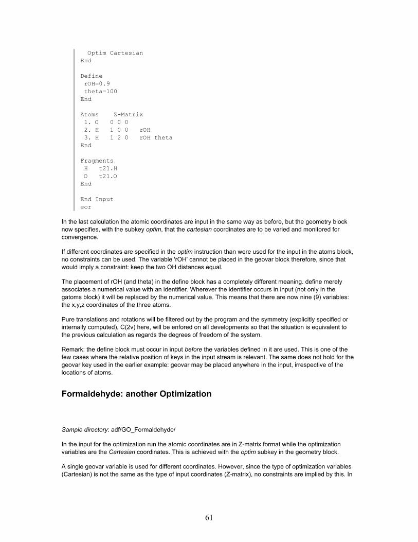
Optim CartesianEnd
DefinerOH=0.9theta=100
End
Atoms Z-Matrix1. O 0 0 02. H 1 0 0 rOH3. H 1 2 0 rOH theta
End
FragmentsH t21.HO t21.O
End
End Inputeor
In the last calculation the atomic coordinates are input in the same way as before, but the geometry blocknow specifies, with the subkey optim, that the cartesian coordinates are to be varied and monitored forconvergence.
If different coordinates are specified in the optim instruction than were used for the input in the atoms block,no constraints can be used. The variable 'rOH' cannot be placed in the geovar block therefore, since thatwould imply a constraint: keep the two OH distances equal.
The placement of rOH (and theta) in the define block has a completely different meaning. define merelyassociates a numerical value with an identifier. Wherever the identifier occurs in input (not only in thegatoms block) it will be replaced by the numerical value. This means that there are now nine (9) variables:the x,y,z coordinates of the three atoms.
Pure translations and rotations will be filtered out by the program and the symmetry (explicitly specified orinternally computed), C(2v) here, will be enfored on all developments so that the situation is equivalent tothe previous calculation as regards the degrees of freedom of the system.
Remark: the define block must occur in input before the variables defined in it are used. This is one of thefew cases where the relative position of keys in the input stream is relevant. The same does not hold for thegeovar key used in the earlier example: geovar may be placed anywhere in the input, irrespective of thelocations of atoms.
Formaldehyde: another Optimization
Sample directory: adf/GO_Formaldehyde/
In the input for the optimization run the atomic coordinates are in Z-matrix format while the optimizationvariables are the Cartesian coordinates. This is achieved with the optim subkey in the geometry block.
A single geovar variable is used for different coordinates. However, since the type of optimization variables(Cartesian) is not the same as the type of input coordinates (Z-matrix), no constraints are implied by this. In
61

fact, the related coordinates do remain equal, but this is because they are symmetry related and theprogram preserves symmetry anyway.
NonLocal gradient corrections (gga: Generalized Gradient Approximation) according to the approach knownas 'Becke' (for exchange) and 'Perdew' (correlation) are included self-consistently with the key xc.
$ADFBIN/adf << eorTitle formaldehyde
GeometryOptim cartes
End
XCGGA Becke Perdew
END
Symmetry C(2v)
Atoms Z-matrix1 O 0 0 0 0.0 0.0 0.02 C 1 0 0 r2 0.0 0.03 H 2 1 0 r3 a3 0.04 H 2 1 3 r3 a3 t4
End
FragmentsC t21.CO t21.OH t21.H
End
Geovarr2 1.94r3 0.95a3 120t4 -180
End
integration 4.5
End Inputeor
Aspirin: an optimization in delocalized coordinates
Sample directory: adf/DelocalGO_aspirin/
Geometry optimization of the aspirin molecule, using the delocalized coordinates.
$ADFBIN/adf <<eorTitle geometry optimization of aspirin in delocalized coordinates
Basis
62

Type DZEnd
GEOMETRYOPTIM DELOCAL
END
ATOMSC 0.000000 0.000000 0.000000C 1.402231 0.000000 0.000000C 2.091015 1.220378 0.000000C 1.373539 2.425321 0.004387C -0.034554 2.451759 0.016301C -0.711248 1.213529 0.005497O -0.709522 3.637718 0.019949C -2.141910 1.166077 -0.004384O -2.727881 2.161939 -0.690916C -0.730162 4.530447 1.037168C -0.066705 4.031914 2.307663H -0.531323 -0.967191 -0.007490H 1.959047 -0.952181 -0.004252H 3.194073 1.231720 -0.005862H 1.933090 3.376356 -0.002746O -2.795018 0.309504 0.548870H -2.174822 2.832497 -1.125018O -1.263773 5.613383 0.944221H -0.337334 4.693941 3.161150H 1.041646 4.053111 2.214199H -0.405932 3.005321 2.572927
END
END INPUT
AuH: Scalar-Relativistic Optimization
Sample directory: adf/RelGO_AuH/
A simple geometry optimization using the scalar relativistic option, implying that relativistic core potentialsmust be generated first (dirac).
$ADFBIN/dirac -n1 < $ADFRESOURCES/Dirac/H$ADFBIN/dirac -n1 < $ADFRESOURCES/Dirac/Au.4d
mv TAPE12 t12.rel
The optimization run is now straightforward (after having created the relativistic basic atoms, not shownhere).
$ADFBIN/adf << eortitle AuH relativistic optimization
integration 5.5
atoms Zmat
63

Au 0 0 0H 1 0 0 1.5end
fragmentsAu t21.AuH t21.Hend
xcGGA Becke Perdew
end
relativisticCorePotentials t12.rel &H 1Au 2end
geometryconvergence grad=1e-4end
end inputeor
The key COREPOTENTIALS is used as block key and it has an argument ('t12.rel'). Consequently thecontinuation character (&) is used. Note that the order of DIRAC runs, to create the relativistic corepotentialsfile TAPE12, determines that in the key block to the CorePotentials key, the H atom must relate to the firstsection on TAPE12 and the Gold atom to the second section.
H2O: restraint Geometry Optimization
Sample directory: adf/GO_restraint/
The restraint does not have to be satisfied at the start of the geometry optimization. An extra force is addedto restrain the bond length, angle, or dihedral angle to a certain value.
Example for angle restraint
$ADFBIN/adf << eortitle WATER geometry optimization with angle restraint
ATOMS1.O 0.001356 0.000999 0.0000002.H 0.994442 -0.037855 0.0000003.H -0.298554 0.948531 0.000000
END
BASISType DZP
END
INTEGRATION 4 4
64

RESTRAINTANGLE 3 1 2 125.0
END
GEOMETRYEND
endinputeor
Example for bond length restraint
$ADFBIN/adf << eortitle WATER Geometry Optimization with bond length restraint
ATOMS1.O 0.001356 0.000999 0.0000002.H 0.994442 -0.037855 0.0000003.H -0.298554 0.948531 0.000000
END
BASISType DZP
END
INTEGRATION 4 4
RESTRAINTDIST 1 2 1.03DIST 1 3 1.03
END
GEOMETRYEND
endinputeor
Example for dihedral angle restraint
$ADFBIN/adf << eorTitle Restraining dihedral of ethane
SYMMETRY NOSYM
ATOMS1.C -0.004115 -0.000021 0.0000232.C 1.535711 0.000022 0.0000083.H -0.399693 1.027812 -0.0000824.H -0.399745 -0.513934 0.8901395.H -0.399612 -0.513952 -0.8901566.H 1.931188 0.514066 0.8901407.H 1.931432 0.513819 -0.8901218.H 1.931281 -1.027824 0.000244
END
INTEGRATION 4 4
65

RESTRAINTDIHED 6 2 1 3 20.00
END
BASIStype DZP
END
GEOMETRYEND
endinputeor
H2O: constraint Geometry Optimization
Sample directory: adf/GO_constraints/
The key CONSTRAINTS can only be used in case of the New branch for optimization of coordinates. Theinput for this key is very similar to that of the RESTRAINT keyword. The key CONSTRAINTS can, however,also be used to constrain Cartesian coordinates. Note that the key RESTRAINT and freezing of coordinateswith the GEOVAR key can also be used in the New branch for optimization of coordinates. In ADF2007 theNew branch for optimization can only be used in geometry optimizations and transition state searches. Notethat the before ADF2008.01 the key CONSTRAINTS was called NEWCONSTRAINTS.
The constraints do not have to be satisfied at the start of the geometry optimization.
Example for angle restraint
$ADFBIN/adf << eortitle WATER geometry optimization with angle constraintATOMS
1.O 0.001356 0.000999 0.0000002.H 0.994442 -0.037855 0.0000003.H -0.298554 0.948531 0.000000
ENDBASISType DZP
ENDINTEGRATION 4 4CONSTRAINTS
ANGLE 3 1 2 125.0ENDGEOMETRY
OPTIM DELOCALENDendinputeor
Example for fixed-atom constraint. Note that the optimization should be done in Cartesian.
$ADFBIN/adf << eortitle WATER geometry optimization with fixed-atom constraint
66

ATOMS1.O 0.001356 0.000999 0.0000002.H 0.994442 -0.037855 0.0000003.H -0.298554 0.948531 0.000000
ENDBASISType DZP
ENDINTEGRATION 4 4SYMMETRY NOSYMCONSTRAINTS
ATOM 1 0.0 0.0 0.0ATOM 2 1.0 0.0 0.0
ENDGEOMETRY
OPTIM CARTESIANBRANCH NEW
ENDendinputeor
Example for bond length restraint.
$ADFBIN/adf << eortitle WATER Geometry Optimization with bond length constraintATOMS
1.O 0.001356 0.000999 0.0000002.H 0.994442 -0.037855 0.0000003.H -0.298554 0.948531 0.000000
ENDBASISType DZP
ENDINTEGRATION 4 4CONSTRAINTS
DIST 1 2 1.03DIST 1 3 1.03
ENDGEOMETRY
OPTIM CARTESIANBRANCH NEW
ENDendinputeor
Example for dihedral angle restraint
$ADFBIN/adf << eorTitle Constraining dihedral of ethaneSYMMETRY NOSYMATOMS
1.C -0.004115 -0.000021 0.0000232.C 1.535711 0.000022 0.0000083.H -0.399693 1.027812 -0.0000824.H -0.399745 -0.513934 0.8901395.H -0.399612 -0.513952 -0.8901566.H 1.931188 0.514066 0.8901407.H 1.931432 0.513819 -0.890121
67

8.H 1.931281 -1.027824 0.000244ENDINTEGRATION 4 4CONSTRAINTS
DIHED 6 2 1 3 20.00ENDBASIS
type DZPENDGEOMETRY
OPTIM DELOCALENDendinputeor
Example for Block constraint (with a dihedral constraint).
$ADFBIN/adf << eorTitle Block constraints (with a dihedral constraint)SYMMETRY NOSYMATOMS
1.C -0.004115 -0.000021 0.000023 b=b12.C 1.535711 0.000022 0.000008 b=b23.H -0.399693 1.027812 -0.000082 b=b14.H -0.399745 -0.513934 0.890139 b=b15.H -0.399612 -0.513952 -0.890156 b=b16.H 1.931188 0.514066 0.890140 b=b27.H 1.931432 0.513819 -0.890121 b=b28.H 1.931281 -1.027824 0.000244 b=b2
ENDINTEGRATION 4 4CONSTRAINTS
DIHED 6 2 1 3 20.00BLOCK b1BLOCK b2
ENDBASIS
type DZPENDGEOMETRY
OPTIM DELOCALENDendinputeor
LiF: optimization with an external electric field or point charges
Sample directory: adf/GO_LiF_Efield/
In the first example a geometry optimization is performed with an external homogeneous electric field. In thesecond example a geometry optimization is performed with an external point charges
68

Note that SYMMETRY NOSYM should be used. In case of point charges it is important to use the QPNEARsubkeyword of the INTEGRATION key with a large enough value that would include some of the pointcharges.
$ADFBIN/adf << eorTitle LiF Cartesian Geometry Optimization in the presence of electricfieldSymmetry NOSYMAtoms
F 0.000000 0.800000 0.000000Li 0.000000 -0.800000 0.000000
EndBasisType TZPCore Small
EndGeometry
Optim CartesianBranch NewConverge 0.0000001Iterations 100
EndEfield 0.0 0.0 0.01
End Inputeor$ADFBIN/adf << eorTitle LiF Cartesian Geometry Optimization in the presence of point chargesSymmetry NOSYMAtoms
F 0.000000 0.800000 0.000000Li 0.000000 -0.800000 0.000000
EndBasisType TZPCore Small
EndGeometry
Optim CartesianBranch NewConverge 0.001Iterations 100
EndEfield &0.0 0.0 5.3 0.50.0 0.0 -5.3 -0.5Endintegration
qpnear 20endEnd Inputeor
CH2O: excited state geometry optimization with a constraint
69

Sample directory: adf/EGO_CH2O_trip_constr/
Example for an excited triplet state geometry optimization with a constraint included.
Needed for such excited state optimizations are the key EXCITATIONS (to calculate excitation energies),the key GEOMETRY (to do a geometry optimization) and the key EXCITEDGO (to select for whichexcitation a geometryy optimization should be performed). In this case a Z-matrix input for the coordinates isused, and a constraint is used using the GEOVAR keyword.
$ADFBIN/adf <<eoratoms zmatrix
C 0 0 0 0.0 0.0 0.0O 1 0 0 R 0.0 0.0H 1 2 0 1.0 110.0 0.0H 1 2 3 1.0 110.0 170.0
end
XCEND
GEOVARR=1.2 F
END
GEOMETRYEND
BASISTYPE DZCORE NONEend
excitationsDAVIDSONLOWEST 5onlytripletend
EXCITEDGOSTATE A'' 1TRIPLETOUTPUT=2
end
SYMMETRY C(S)
eor
Transition States, Linear Transits, Intrinsic ReactionCoordinates
HCN: LT, Frequencies, TS, and IRC
70

Sample directory: adf/HCN/
Summary
• For a sequence of intermediates, each defined by a fixed angle H-C-N between the linearextremesHCN and CNH, the remaining geometrical parameters are optimized, giving a Linear Transitpoint-by-point scan of the energy curve of the Hydrogen atom travelling from one end of the CNfragment to the other. This is a useful way to get a reasonable first guess of the Transition State.
• At the approximate TS a Frequencies calculation is performed to obtain a fairly accurate Hessianfor the next calculation.
• A TS search is carried out, using the computed Hessian. As variation, the TS search is repeated,firstwith the automatic (internal) Hessian (based on force fields) and then also with a constraintapplied.
• A full IRC scan of the full path, starting from the TS, down to the two minima.
LT
The first calculation is a Linear Transit where the Hydrogen atom moves from one side of CN to the other bya parameterized step-by-step change of the angle H-C-N. The other coordinates of the system are optimizedalong the path.
In the atoms block, one coordinate value is represented by an identifier (th). In the geovar block this isasssigned two values, implying that it is a Linear Transit parameter. The initial and final values for theparameter are given.
Since the geometry block does not have OPTIM SELECTED, all other coordinates are optimized for each ofthe 10 Linear Transit points.
The subkey iterations in the geometry block carries two arguments: the first is the maximum number ofoptimization steps (per LT point). The second is the number of LT points to compute in this run: 4. Thisimplies that only a part of the 10-point path defined by the LT parameter(s) will be scanned. The remainderwill be done in a follow-up run to illustrate usage of the restart facility.
$ADFBIN/adf <<eorTitle HCN Linear Transit, first partNoPrint SFO, Frag, Functions, Computation
Atoms Internal1 C 0 0 0 0 0 02 N 1 0 0 1.3 0 03 H 1 2 0 1.0 th 0
End
BasisType DZP
End
Symmetry NOSYM
Integration 6.0 6.0
GeometryBranch Old
71

LinearTransit 10Iterations 30 4Converge Grad=3e-2, Rad=3e-2, Angle=2
END
Geovarth 180 0
End
End Inputeor
mv TAPE21 t21.LTrm logfile
The NoPRINT key turns off a lot of default output. There are several PRINT and NOPRINT options; see theUser's Guides for details.
Since the geometry changes from linear to planar (and finally back to linear again), the symmetry must begiven explicitly in the input file. Otherwise the program would find a C(lin) symmetry for the initial geometryand assume that this symmetry is preserved throughout. This would of course result in an error abort whenthe first LT step is carried out, breaking the linear symmetry.
The here specified symmetry (NOSYM: no symmetry at all) is not the true symmetry of the complete pathC(s) but a subgroup. It is always allowed to specify a lower symmetry than the actually present symmetry.Such may be necessary (for instance when the true symmetry cannot be handled by adf) or in special casesrequired for reasons of analysis. Generally speaking, however, we recommend to use the highest symmetrypossible (given the case at hand and taking into account the symmetries recognizable by ADF) to boostperformance.
Convergence thresholds in the geometry block are set less tight than the defaults: we need only areasonable estimate of the path, but no highly converged geometries.
At the end of the run the tape21 result file is saved and renamed t21.LT to serve as restart file for the follow-up calculation.
LT continuation
$ADFBIN/adf <<eorTitle HCN Linear TransitNoPrint SFO,Frag,Functions,Computation
Restart t21.LT
FragmentsN t21.NC t21.CH t21.H
End
Atoms Internal1 C 0 0 0 0 0 02 N 1 0 0 1.3 0 03 H 1 2 0 1.0 th 0
End
72

symmetry NOSYM
Integration 6.0 6.0
GeometryBranch OldLinearTransit 10Converge Grad=3e-2, Rad=3e-2, Angle=2
END
Geovarth 180 0
End
End Inputeor
rm TAPE21 logfile
From the restart file, supplied with the key restart, the program reads off that the first 4 points of the LT pathhave been done already and the scan is continued with LT point #5. The same path definition is suppliedagain, including the original starting values for the coordinates. The actual starting coordinates (for LT point#5) are read from the restart file. The input values, however, serve to define and verify consistency of thedefined LT path and must therefore be supplied correctly.
The key noprint is used to suppress major parts of standard output: all information pertaining to the sfoanalysis, all build-from-fragments information, and the lists of elementary functions in the basis sets and fitsets.
Frequencies at the estimated Transition State
From the results of the Linear Transit run we can sketch the energy barrier that H passes over when goingfrom one side of the molecule to the other. This yields a reasonable guess for the Transition State.
To check that the so-obtained estimate is adequate we compute the frequencies in that geometry: one ofthem should be imaginary.
Apart from serving as a check that the TS estimate is not too bad, the computed Hessian will also serve inthe follow-up calculation to obtain the true TS.
$ADFBIN/adf <<eorTitle HCN Frequencies in LT max (approx), moderate precisionNoPrint SFO,Frag,Functions,Computation
Integration 6.0 6.0
FragmentsN t21.NC t21.CH t21.H
End
Atoms Internal1 C 0 0 0 0 0 02 N 1 0 0 1.186 0 0
73

3 H 1 2 0 1.223 70 0End
GeometryFrequencies
End
End Inputeor
mv TAPE21 t21.Freq
Inspection of the output file shows that one of the frequencies is imaginary, as expected (printed asnegative), signalling the proximity of the Transition State.
The TAPE21 result file of the calculation is renamed and saved. Later we will use it as a 'restart' file for a TSsearch, namely to supply the computed Hessian as the initial 'guess' of the Hessian in the (TS) optimizationrun.
TS search
Now carry out the Transition State search, starting from the lt-derived guess.
In this first attempt to find the TS, no use is made of the tape21 result file from the Frequencies run. That willbe done in the next calculation.
$ADFBIN/adf <<eorTitle HCN Transition State, automatic initial HessianNoPrint SFO,Frag,Functions,Computation
Integration 6.0 6.0
Atoms Internal1 C 0 0 0 0 0 02 N 1 0 0 1.186 0 03 H 1 2 0 1.223 70 0
End
FragmentsN t21.NC t21.CH t21.H
End
GeometryTransitionState
End
End Inputeor
rm TAPE21 logfile
The TS-search run type is specified in the geometryblock.
No symmetry is specified; the program determines the symmetry to be C(s) and consequently carries out thets search in that symmetry.
74

TS search, using the Hessian from the Frequencies run
$ADFBIN/adf <<eorTitle HCN Transition State, initial Hessian from Freq runNoPrint SFO,Frag,Functions,Computation
Restart t21.FreqSave TAPE13
Integration 6.0 6.0
Atoms Internal1 C 0 0 0 0 0 02 N 1 0 0 1.186 0 03 H 1 2 0 1.223 70 0
End
FragmentsN t21.NC t21.CH t21.H
End
GeometryTransitionState
End
End Inputeor
mv TAPE13 t13.TSrm TAPE21 logfile
The CheckPoint file TAPE13, at normal termination automatically deleted by the program, is here saved,using the SAVE key. TAPE13 is as good a restart file as TAPE21 is, but it is a lot smaller. TAPE21 containsa large amount of information for analysis purposes, while TAPE13 contains essentially only restart-typedata.
The input is identical to the previous one, except for the restart file. This is used here to provide the Hessiancomputed in the Frequencies run as the start-up Hessian for the ts optimization. At the same time the atomiccoordinates are read off from the restart file and override the values in the input file. This latter aspect couldhave been suppressed; see the User's Guide for using the restart key.
Constrained TS search
Finally the ts search where one coordinate is kept frozen, to illustrate a constrained optimization.
$ADFBIN/adf <<eorTitle HCN constrained TS searchNoPrint SFO,Frag,Functions,Computation
Restart t21.Freq
Integration 6.0 6.0
Atoms Internal
75

1 C 0 0 0 0 0 02 N 1 0 0 rNC 0 03 H 1 2 0 1.223 70 0
End
GeoVarrNC=1.186 F
End
FragmentsN t21.NC t21.CH t21.H
End
GeometryTransitionState
End
End Inputeor
rm TAPE21 logfilerm t21.Freq
The geovar key specifies that the nc distance, rNC has the initial value 1.15 and remains frozen ('F').
The fact that the optimization is now carried out in a different subspace of atomic coordinates does notprevent us from using the t21.Freq restart file to supply the initial Hessian.
IRC scan of the reaction path
The IRC calculation is split in three steps, to illustrate the Restart facility applied to the IRC functionality.
In the first only a few points are computed, along one of the two paths leading from the TS to the adjacentminima. Since no explicit directives are given in the input to specify the direction of the first path, the so-called 'forward' path is taken. The definition of which is 'forward' and which is 'backward' is in fact quitearbitrary and is determined by the program. See the User's Guide for details.
The saved TAPE13 file from one of the TS calculations is used as restart file. This provides (a) the optimizedcoordinates of the TS as starting point, (b) the initial Hessian to guide the point-by-point optimizations alongthe IRC path, and (c) the eigenvector of the lowest Hessian eigenvalue to define the initial direction of theIRC path.
The TAPE13 file from this partial IRC scan is saved to serve as start-up file for the next calculations, whichwill continue the IRC scan.
In the Geometry key block, the run type is set to IRC and the 'Points' option is used to limit the number ofIRC points to compute.
$ADFBIN/adf << eorTitle HCN IRC partial path (forward)NoPrint SFO,Frag,Functions, Computation
Integration 6.0 6.0
76

Restart t13.TSSave TAPE13
Atoms Internal1 C 0 0 0 0 0 02 N 1 0 0 1.186 0 03 H 1 2 0 1.223 70 0
End
FragmentsN t21.NC t21.CH t21.H
End
GeometryIRC Points=5
End
End Inputeor
mv TAPE13 t13.IRC_1rm TAPE21 logfile
The IRC is continued in the next calculation, using the TAPE13 file from the previous one as restart file.From this file, the program reads the IRC path information computed sofar. By default, it would continue onthe 'forward' path, since that was not yet finished. However, in the Geometry key block, we now specify notonly that a limited number of points is to be computed in this run (5 again), but we instruct the program alsoto compute only points on the 'backward' path.
$ADFBIN/adf << eorTitle HCN IRC partial part (backward)NoPrint SFO,Frag,Functions, Computation
Restart t13.IRC_1Save TAPE13
Integration 6.0 6.0
Atoms Internal1 C 0 0 0 0 0 02 N 1 0 0 1.186 0 03 H 1 2 0 1.223 70 0
END
FragmentsN t21.NC t21.CH t21.H
End
GeometryIRC Points=5 Backward
End
End Input
77

eor
mv TAPE13 t13.IRC_2rm TAPE21 logfile
In the third IRC run, the IRC scan is finished. We start with the TAPE13 file from the previous run and set amaximum of 70 IRC points to compute (which turns out to be sufficient for the complete IRC scan). Theprogram starts on the forward path, continuing where the first (not the previous) had stopped after 5 points,completes the forward path, and then continues on the backward path, starting where the second IRC runhad stopped. Both paths are finished and a summary of the path characteristics is printed in the final part ofthe output.
$ADFBIN/adf << eorTitle HCN IRC completionNoPrint SFO,Frag,Functions, Computation
Restart t13.IRC_2
Integration 6.0 6.0
Atoms Internal1 C 0 0 0 0 0 02 N 1 0 0 1.186 0 03 H 1 2 0 1.223 70 0
End
FragmentsN t21.NC t21.CH t21.H
End
GeometryIRC Points=70
End
End Inputeor
HCN: transition state search with the CINEB method
Sample directory: adf/HCN_CINEB/
This example demonstrates the use of the Nudged Elastic Band method in ADF for finding a transition stateof the HCN isomerisation reaction. A shell script used to run the example calculation is shown below:
$ADFBIN/adf <<eorTITLE Test of the CI-NEB method
SYMMETRY C(S)
NOPRINT SCF SFOUNITS
length Angstrom
78

angle DegreeEND
ATOMS1.C 0.000000 0.000000 0.0000002.N XN 0.000000 0.0000003.H XH YH 0.000000
END
GEOVARXN 1.180 1.163XH 2.196 1.831 1.006 0.105 -0.718 -1.078YH 0.000 0.799 1.122 1.163 0.813 0.000END
BASISEND
GEOMETRYCINEB 9iterations 150OPTIM selectedconverge grad=0.001nebspring 1 0.06
END
integration 4.0
SCFConvergence 0.00000001
END
eor
A few important points to note:
• Symmetry is set to Cs explicitly because all images must have the same symmetry but symmetryof the reaction products is higher, C∞. Thus, it is necessary to lower the overall symmetry to matchthe lowest.
• In the GEOVAR section, there are six values specified for the coordinates of the hydrogen atom.Thisi is necessary in order to bring the initial guess for the reaction path closer to the final result.Moreover, if only two values for YH were specified (0.0 and 0.0) then the hydrogen atom would be"dragged" along the C-N bond leading to unrealistic geometries and, eventually, to a failure.
• In the GEOMETRY section of the input, the number of NEB images is set to 9; the convergencecriterion is lowered to 0.001; optimization of only the coordinates specified in the GEOVAR blockis requested;
• the NEB spring parameter is set to a constant (energy-independent) value of 0.06 a.u.. The choiceof the parameter depends on the stiffness of the bonds involved in the reaction and the value ofthe parameter should, in principle, be of about the same magnitude as the Hessian eigenvalue forthe coordinates participating in the reaction.
C2H6 internal rotation: TS search using partial Hessian
Sample directory: adf/TS_C2H6/
79

Frequently when searching for a transition state, one needs an accurate second derivatives matrix, aHessian. An exact Hessian may be obtained analytically but this may be very expensive for large molecules.In such cases it may be beneficial to calculate Hessian matrix elements only for atoms directly involved inthe reaction for which a transition state is sought for. The rest of the Hessian can then be approximatedusing a cheaper method.
In this example, a saddle point of the ethane internal rotation around C-C bond is found. In principle, onlyhydrogen atoms contribute to the normal mode we are interested in. Therefore we calculate a partialHessian matrix including hydrogen atoms only. For this purpose, the AnalyticalFreq block key is used. In thisblock, a NUC keyword is added specifying that the second derivatives are calculated for atom 3 (and itssymmetry-equivalents) only. Note that the Hessian matrix elements between symmetry-equivalent atoms, forexample between 3,H and 4.H are also calculated. The rest of the matrix is estimated using the defaultmethod.
$ADFBIN/adf <<eorTITLE Ethane transition state search using partial Hessian
ATOMS1 C 0.000000000000 0.000000000000 0.7676854650312 C 0.000000000000 0.000000000000 -0.7676854650313 H 0.964354016767 0.347635559279 1.1771282714504 H -0.181115782790 -1.008972856410 1.1771282714505 H -0.783238233981 0.661337297125 1.1771282714506 H -0.500471876676 0.894626767091 -1.1771282714507 H -0.524533568868 -0.880734742626 -1.1771282714508 H 1.025005445540 -0.013892024465 -1.177128271450END
BASIStype DZcore LargeEND
AnalyticalFreqNUC 3
End
INTEGRATION 5.0 5.0 5.0eor
After the Hessian is calculated, the resulting TAPE21 file is used for a subsequent transition state search:
mv TAPE21 ethane-frq.t21
$ADFBIN/adf <<eorTITLE Ethane transition state search using partial Hessian
ATOMS1 C 0.000000000000 0.000000000000 0.7676854650312 C 0.000000000000 0.000000000000 -0.7676854650313 H 0.964354016767 0.347635559279 1.1771282714504 H -0.181115782790 -1.008972856410 1.1771282714505 H -0.783238233981 0.661337297125 1.1771282714506 H -0.500471876676 0.894626767091 -1.1771282714507 H -0.524533568868 -0.880734742626 -1.1771282714508 H 1.025005445540 -0.013892024465 -1.177128271450END
80

FragmentsH t21.HC t21.C
END
GEOMETRYsmooth conservepointsTransitionState mode=1optim All Cartesianiterations 30step rad=0.15hessupd BOFILLconverge e=1.0e-4 grad=1.0e-3 rad=1.0e-3
END
RESTART ethane-frq.t21
INTEGRATION 5.0 5.0 5.0eor
Important note: care should be taken to specify correct mode in the TransitionState keyword. Because asignificant part of the Hessian will not be calculated exactly, it is possible that it will have more than onenegative eigenvalue, in which case the one we are interested in may not be the first one. In such a case,one needs to specify the correct mode number in the TransitionState keyword.
CH4+HgCl2⇔CH3HgCl+HCl: a TS search
Sample directory: adf/RelTS_CH4_HgCl2/
A Transition State calculation, including scalar relativistic terms in the Hamiltonian.
First the relativistic core potentials are generated.
$ADFBIN/dirac -n1 < $ADFRESOURCES/Dirac/Hg.4d$ADFBIN/dirac -n1 < $ADFRESOURCES/Dirac/Cl.2p$ADFBIN/dirac -n1 < $ADFRESOURCES/Dirac/C.1s$ADFBIN/dirac -n1 < $ADFRESOURCES/Dirac/H
mv TAPE12 t12.rel
Then the (relativistic) Create runs.
$ADFBIN/adf << eorcreate Hg $ADFRESOURCES/TZP/Hg.4drelativisticcorepotentials t12.rel &Hg 1endend inputeor
mv TAPE21 t21.Hg
81

$ADFBIN/adf << eorcreate Cl $ADFRESOURCES/TZP/Cl.2prelativisticcorepotentials t12.rel &Cl 2endend inputeor
mv TAPE21 t21.Cl
$ADFBIN/adf << eorcreate C $ADFRESOURCES/TZP/C.1srelativisticcorepotentials t12.rel &C 3endend inputeor
mv TAPE21 t21.C
$ADFBIN/adf << eorcreate H $ADFRESOURCES/TZP/Hrelativisticcorepotentials t12.rel &H 4endend inputeor
mv TAPE21 t21.H
In the first Create run (Hg) the CorePotentials key could have been used in its simple form, but in the second(and third and fourth, omitted here) the block form is required to identify the appropriate section on TAPE12for the atom at hand. In the first case we could have relied on the default: the first section on TAPE12 for thefirst (in this case: only) atom type.
Note that even for H, which obviously has no frozen core at all, we specify the TAPE12 corepotentials fileand indicate the appropriate section for H. The reason is that TAPE12 contains not only the (frozen) core,but also the total atomic (relativistic) potential.
Finally the TS run.
$ADFBIN/adf << eorTITLE Transition State: CH4 + HgCl2 ↔ CH3HgCl + HCl
noprint sfo,fragprint atdist
GEOMETRYTransitionState
END
82

relativisticcorepotentials t12.rel &C 3Hg 1Cl 2H 4end
XClda VWN StollEND
DEFINErHg = 2.30rX1 = 2.35rX2 = 2.90rH1 = 1.10rH2 = 1.10rH3 = 1.40
aX1 = 160aX2 = 70aH1 = 100aH2 = 140aH3 = 65
dH = 60END
ATOMS Z-Matrix1. C 0 0 0 0. 0. 0.2. Hg 1 0 0 rHg 0. 0.3. Cl 2 1 0 rX1 aX1 0.4. H 1 2 3 rH1 aH1 dH5. H 1 2 3 rH1 aH1 -dH6. H 1 2 3 rH2 aH2 180.7. H 1 2 3 rH3 aH3 180.8. Cl 2 1 3 rX2 aX2 180.
END
FRAGMENTSHg t21.HgC t21.CH t21.HCl t21.Cl
END
endinputeor
For the density-functional the Local Density approximation is used (no GGA corrections), with a correlationcorrection term due to Stoll (see the User's Guide).
At each geometry cycle the interatomic distance matrix is printed (print atdist).
83

The initial geometry is a reasonable but not very accuracte estimate of the Transition State. The programneeds quite a few cycles to converge, which is rather typical for ts searches: they are a lot more tricky andfail more often than a simple minimization.
F-+CH3Cl: TS reaction coordinate
Sample directory: adf/TSRC_SN2/
With the TSRC key one can specify a reaction coordinate along which the transition state is sought for. Thisfeature is especially useful when an accurate Hessian is not available.
This example tries to find the TS for the SN2 reaction of F- + CH3Cl ⇔ CH3F + Cl-
$ADFBIN/adf << eorTitle TransitionState search for Sn2 reaction of F- + CH3ClANALYTICALFREQENDXCLDA VWNGGA OPBE
ENDTSRC
dist 1 5 1.0dist 1 6 -1.0
ENDATOMS
C 0.000000 0.000000 0.000000H -0.530807 0.919384693 0.012892H -0.530807 -0.919384693 0.012892H 1.061614 0.000000 0.012892Cl 0.000000 0.000000 -2.124300F 0.000000 0.000000 2.019100
ENDGeometryTS
EndBASIStype TZ2Pcore NONEcreateoutput none
ENDINTEGRATION 6.0 6.0Charge -1endinputeor
H2O: constraint Linear Transit
Sample directory: adf/LT_constraint/
84

The LINEARCONSTRAINTS keyword allows geometry optimizations (old branch) with constraints definedby arbitrary linear combinations of (internal) coordinates. The constraint has to be satisfied at the start of thegeometry optimization. Note that the before ADF2008.01 the key LINEARCONSTRAINTS was calledCONSTRAINT.
Example for bond length constraint, where at the start of the linear transit rOH1=R1=1.0, and rOH2=R2=1.5,such that (-1.0)*R1+(1.0)*R2=0.5, and in the final geometry -R1+R2=0.0 (Reactcoord 0.5 0.0)
$ADFBIN/adf << eortitle constraint keywordXC
GGA Becke PerdewEND
GeometryBranch OldLinearTransit 6
End
Integration 5.0
Atoms InternalO 0 0 0H 1 0 0 R1H 1 2 0 R2 109.9End
GeoVarR1 =1.R2 =1.5
End
LinearConstraintsReactCoord 0.5 0.0R1 -1.0R2 1.0
SubEndEnd
BasisType DZP
End
end inputeor
H2O: (non-)Linear Transit
Sample directory: adf/Transit_H2O/
In ADF2008.01 a transit calculation option has been added in the new optimization branch. This is capableof performing both linear transits, and non-linear transits, and is the default when the LINEARTRANSIT orTRANSIT sub-block is included in the 'Geometry' block.
85

The new transit code works differently to the old: the transit is represented as a sequence of constrainedoptimizations. A 'Constraints' block is used to delineate the constraints applied at each stage of the transit.
Non-linear transits are possible, and can even be combined with linear transits in other coordinates. Toperform a non-linear transit in a particular coordinate, explicit values must be given.
$ADFBIN/adf << eorTitle WATER Transit (non-linear), with the new optimizer branchAtoms
O 0.000000 0.000000 0.000000H 0.000000 -0.689440 -0.578509H 0.000000 0.689440 -0.578509
EndSymmetry NOSYMConstraints
dist 1 2 0.8 1.0 1.25 1.5angle 2 1 3 start=100.0 end=120.0
EndBasisType SZCore Large
EndIntegration 4.0 2.0Geometry
Transit 4Optim DelocConverge 0.0001
EndEnd Input
In the example above, 4 values are given for the distance between atoms 1 and 2. This distance constraintwill be applied simultaneously with the linear transit constraints for the angle, with other degrees of freedomoptimized at each stage of the transit.
Finally, it should be pointed out that 'partial constraints' are used by default in the transit calculations. Theseconstraints are not required to be fully met at each intermediate geometry, but are fully met at the convergedgeometries. You can use fully converged constraints by supplying the FULLCONVERGE option to the'Constraints' subblock of the 'Geometry' block (not to be confused with the 'Constraints' block at root level).
Quild
CO: Quild B3LYP geometry optimization
Sample directory: quild/quild_b3lyp_opt/
This example shows how to use the program Quild for a B3LYP geometry optimization, where only the bondenergy of the ADF calculation is used.
B3LYP post-SCF
The subkey NUMGRAD of the block key QUILD is 1, which means that the ADF bond energy is read from thepost-SCF METAGGA scheme. The subkey SMETAGGA of the block key QUILD has as argument a string for
86

the functional (B3LYP(VWN5)), which should be exactly the same as is written on output if the METAGGAkeyword is used.
$ADFBIN/quild << eortitle Geometry optimizationEPRINTSFO NOEIG NOOVL
ENDXCGGA BLYP
ENDATOMSO .000000 .000000 .000000C .000000 .000000 1.128100ENDBASIStype DZcore NONE
ENDGEOMETRYENDSCFdiis ok=0.01converge 1.0e-5 1.0e-5
ENDQUILD
cvg_grd 1.0e-4numgrad 1SMETAGGA B3LYP(VWN5)
ENDMETAGGAHFEXCHANGEINTEGRATION 5.0 5.0endinputeor
B3LYP SCF
In the next calculation the optimization is done with B3LYP as SCF functional. The difference with theprevious calculation is is in blue. The subkey NUMGRAD of the block key QUILD is 2, which means that thestandard ADF bond energy is used.
$ADFBIN/quild << eortitle Geometry optimizationEPRINTSFO NOEIG NOOVL
ENDXCHYBRID B3LYP
ENDATOMSO .000000 .000000 .000000C .000000 .000000 1.128100ENDBASIStype DZ
87

core NONEENDGEOMETRYENDSCFdiis ok=0.01converge 1.0e-5 1.0e-5
ENDQUILD
cvg_grd 1.0e-4numgrad 2
ENDINTEGRATION 5.0 5.0endinputeor
H2O dimer: Quild QM/MM geometry optimization
Sample directory: quild/quild_qmmm_water2/
This example shows how to use the program Quild for a QM/MM geometry optimization of the water dimer.
$ADFBIN/quild << eorTITLE QM/MM calculation setup by pdb2adf: M.Swart, 2005
GEOMETRYEND
ATOMSO 0.0000 0.0000 0.0000H -0.5220 0.2660 -0.7570H -0.5220 0.2660 0.7570O 0.0000 -3.2000 0.0000H 0.0570 -2.2440 0.0000H 0.9110 -3.4950 0.0000END
QUILDNR_REGIONS=2
INTERACTIONSTOTAL description 1REPLACE region 1 description 3 for description 2
SUBEND
REGION 11-3
SUBENDREGION 2
4-6SUBEND
DESCRIPTION 1 NEWMMQMMM
88
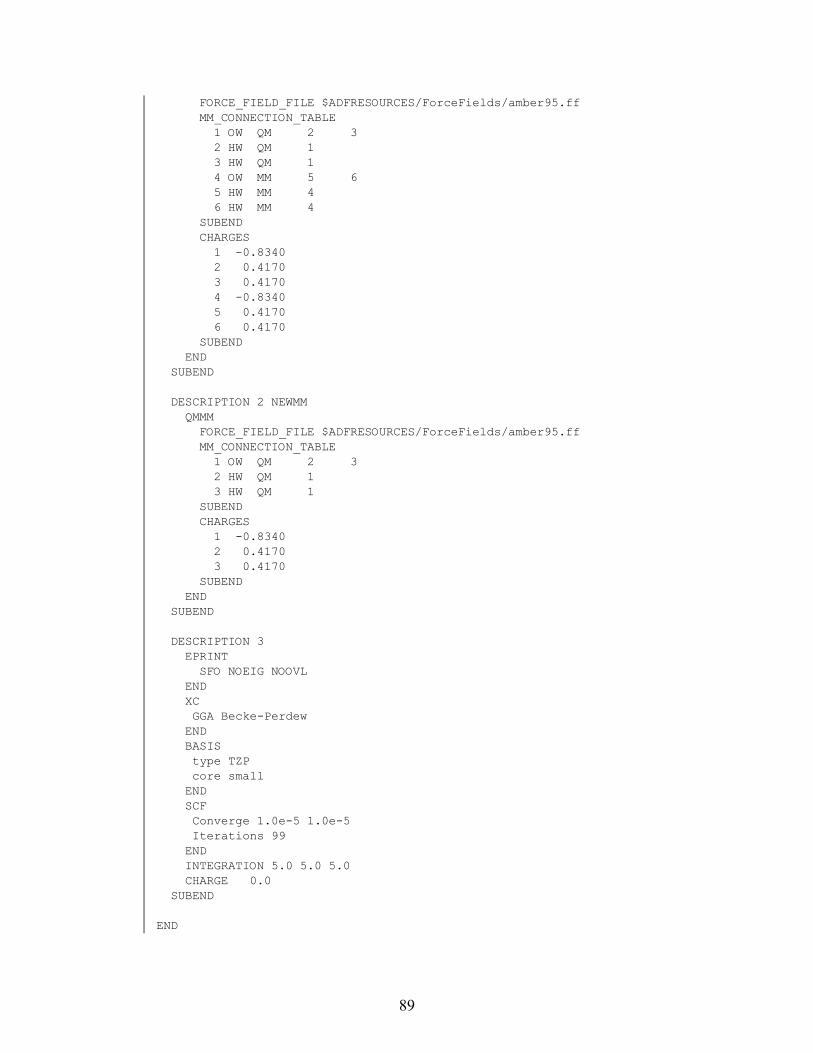
FORCE_FIELD_FILE $ADFRESOURCES/ForceFields/amber95.ffMM_CONNECTION_TABLE
1 OW QM 2 32 HW QM 13 HW QM 14 OW MM 5 65 HW MM 46 HW MM 4
SUBENDCHARGES
1 -0.83402 0.41703 0.41704 -0.83405 0.41706 0.4170
SUBENDEND
SUBEND
DESCRIPTION 2 NEWMMQMMM
FORCE_FIELD_FILE $ADFRESOURCES/ForceFields/amber95.ffMM_CONNECTION_TABLE
1 OW QM 2 32 HW QM 13 HW QM 1
SUBENDCHARGES
1 -0.83402 0.41703 0.4170
SUBENDEND
SUBEND
DESCRIPTION 3EPRINT
SFO NOEIG NOOVLENDXCGGA Becke-Perdew
ENDBASIStype TZPcore small
ENDSCFConverge 1.0e-5 1.0e-5Iterations 99
ENDINTEGRATION 5.0 5.0 5.0CHARGE 0.0
SUBEND
END
89

ENDINPUTeor
F- + CH3Cl: Quild transition state search
Sample directory: quild/quild_qmmm_water2/
This example shows how to use the program Quild for a transition state search of the SN2 reaction of F- +CH3Cl
$ADFBIN/quild << eorTitle TransitionState search for Sn2 reaction of F- + CH3ClANALYTICALFREQENDXCGGA OPBE
END
QUILDTSRC
dist 1 5dist 1 6
SUBENDEND
ATOMSC 0.000000 0.000000 0.000000H -0.530807 0.919384693 0.112892H -0.530807 -0.919384693 0.112892H 1.061614 0.000000 0.112892Cl 0.000000 0.000000 -2.124300F 0.000000 0.000000 2.019100
ENDGeometryTS
EndBASIStype TZ2Pcore NONE
ENDINTEGRATION 6.0 6.0SCFconverge 1.0e-6 1.0e-6diis ok=0.01iterations 99
ENDCharge -1EPRINTSFO noeig noovl
ENDendinputeor
90
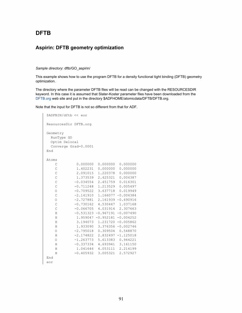
DFTB
Aspirin: DFTB geometry optimization
Sample directory: dftb/GO_aspirin/
This example shows how to use the program DFTB for a density functional tight binding (DFTB) geometryoptimization.
The directory where the parameter DFTB files will be read can be changed with the RESOURCESDIRkeyword. In this case it is assumed that Slater-Koster parameter files have been downloaded from theDFTB.org web site and put in the directory $ADFHOME/atomicdata/DFTB/DFTB.org.
Note that the input for DFTB is not so different from that for ADF.
$ADFBIN/dftb << eor
ResourcesDir DFTB.org
GeometryRunType GOOptim DelocalConverge Grad=0.0001
End
AtomsC 0.000000 0.000000 0.000000C 1.402231 0.000000 0.000000C 2.091015 1.220378 0.000000C 1.373539 2.425321 0.004387C -0.034554 2.451759 0.016301C -0.711248 1.213529 0.005497O -0.709522 3.637718 0.019949C -2.141910 1.166077 -0.004384O -2.727881 2.161939 -0.690916C -0.730162 4.530447 1.037168C -0.066705 4.031914 2.307663H -0.531323 -0.967191 -0.007490H 1.959047 -0.952181 -0.004252H 3.194073 1.231720 -0.005862H 1.933090 3.376356 -0.002746O -2.795018 0.309504 0.548870H -2.174822 2.832497 -1.125018O -1.263773 5.613383 0.944221H -0.337334 4.693941 3.161150H 1.041646 4.053111 2.214199H -0.405932 3.005321 2.572927
Endeor
91

CH3CN_3H2O: DFTB frequency calculation
Sample directory: dftb/DFTB_Freq_CH3CN_3H2O/
This example shows how to use the program DFTB for a density functional tight binding (DFTB) frequencycalculation.
The directory where the parameter DFTB files will be read can be changed with the RESOURCESDIRkeyword. In this case it is assumed that Slater-Koster parameter files have been downloaded from theDFTB.org web site and put in the directory $ADFHOME/atomicdata/DFTB/DFTB.org.
Note that the input for DFTB is not so different from that for ADF.
This example calculation is on a CH3CN molecule surrounded by 3 water molecules. The structure is notoptimized, thus there may be imaginary frequencies. In the output the imaginary frequencies have anegative sign.
$ADFBIN/dftb << eor
ResourcesDir DFTB.org
ATOMSC 1.11496173 0.31854733 0.53703775N 0.59792937 0.63879019 -0.43665677C 1.77005290 -0.09099876 1.76456883H 1.01869497 -0.35318808 2.52004768H 2.39216439 0.72757119 2.14786361H 2.40589405 -0.96472653 1.57420526O -2.09278652 1.16966361 -1.33023377H -1.59202088 1.50609280 -2.09426593H -1.43148181 0.79477801 -0.72038096O 0.90768880 -0.74489752 -3.05331980H 0.82923598 -0.51524973 -2.11150163H 0.68273250 0.06615005 -3.54260509H 0.64422673 1.90218300 -2.26586945O 0.02801757 1.96024309 -3.01706698H -0.85740391 1.75708207 -2.66132398
END
GeometryRunType Frequencies
Endeor
Total energy, Multiplet States, S2, Localized hole, CEBE
H2O: Total Energy calculation
Sample directory: adf/Energy_H2O/
92

If the TOTALENERGY is included the total energy will be calculated.
This example performs single point runs for H2O with PBE/DZP with frozen cores and all-electron andB3LYP/DZP with all-electron and HARTREEFOCK/DZP with all-electron The tests run in C(2v) symmetry.Integration accuracy is 6.0 which should give total energies accurate at least up to 10-4 atomic units. Thekey EXACTDENSITY is used for higher accuracy of the results.
First example:
$ADFBIN/adf <<eorTitle H2O PBE/DZP (frozen core) single point calculationATOMS
O 0.00000 0.00000 0.00000H 0.00000 -0.68944 -0.57851H 0.00000 0.68944 -0.57851
ENDBASIS
Type DZPCore Small
ENDXC
GGA PBEENDINTEGRATION 6.0EXACTDENSITYTOTALENERGYeor
Note that only energy difference comparisons are meaningful. These are the only energies that play a role inchemistry of course, and for this one does not need total energies.
[Cr(NH3)6]3+: Multiplet States
Sample directory: adf/SD_CrNH3_6/
The computation of multiplet states corresponding to an open-shell system can be carried out with ADF byfirst computing the 'Average-of-Configuration' (aoc) state, where all orbitals in the open shell are degenerateand equally occupied. This computation is spin-restricted and serves as a fragment file for the multiplet run,where then different occupation numbers are assigned to the various orbitals in the open shell. Thecorresponding energies are computed in the field of the aoc, which is achieved by not iterating the self-consistency equations to convergence but only computing the orbitals in the initial field.
Since ADF requires that all symmetry-partners in an irreducible representation (irrep) have equaloccupations, the multiplet calculation, where such orbitals are not equally occupied, must be carried out in aformally lower pointgroup symmetry. The pointgroup to select and the appropriate occupation numbers toapply must be worked out by the user 'on paper' in advance. An auxiliary program asf, developed by thegroup of Claude Daul in Fribourg can be used to determine which calculations are needed, and how tocompute the multiplet energies from the results. See the discussion of Multiplet energies in the Theorydocument.
The script starts with the 'creation' of the required basic atoms, N, H, Cr using a fair basis set quality.
The next step is the computation of the ammonia fragment NH3. This is not a crucial step here: the multipletstate computation can equally well be carried out by not using any intermediate compound fragments.
93

However, it illustrates once more how a bigger molecule can be built up from smaller, but not trivialfragments.
$ADFBIN/adf <<eortitle AMMONIANOPRINT sfo,frag,functions
definexH=0.95522523yH=xH*sqrt(3)/2zH=0.3711068end
atomsN 0 0 0H -xH 0 zHH xH/2 -yH zHH xH/2 yH zHend
BasisType TZPCore Small
End
symmetry C(3V)
endinputeor
mv TAPE21 t21.NH3
The input of the atomic coordinates uses expressions, in this case to enforce exact symmetry relations thatwould otherwise require 14-digit input values or some inaccuracy. The symmetry specification is redundant:the program would also find it by itself.
Average-of-Configuration
The next step is to compute the reference state, with respect to which we will later compute the multipletstates. The reference state is the so-called 'Average-of-configuration' (aoc) state. The result file (TAPE21) ofthis calculation will be used as a fragment file.
$ADFBIN/adf <<eortitle Cr(NH3)6 : Average-of-Configuration run
COMMENTusing NH3-fragmentsEND
symmetry D(3d)
scfiterations 25mix 0.15end
94

atomsCr 0.000000 0.000000 0.000000N 0.000000 1.714643 1.212436 f=NH3/1H 0.000000 1.466154 2.206635 f=NH3/1H -0.827250 2.293404 1.036727 f=NH3/1H 0.827250 2.293404 1.036727 f=NH3/1N -1.484924 -0.857321 1.212436 f=NH3/2H -1.269726 -0.733077 2.206635 f=NH3/2H -1.572521 -1.863121 1.036727 f=NH3/2H -2.399771 -0.430282 1.036727 f=NH3/2N 1.484924 -0.857321 1.212436 f=NH3/3H 1.269726 -0.733077 2.206635 f=NH3/3H 2.399771 -0.430282 1.036727 f=NH3/3H 1.572521 -1.863121 1.036727 f=NH3/3N 0.000000 -1.714643 -1.212436 f=NH3/4H 0.000000 -1.466154 -2.206635 f=NH3/4H 0.827250 -2.293404 -1.036727 f=NH3/4H -0.827250 -2.293404 -1.036727 f=NH3/4N 1.484924 0.857321 -1.212436 f=NH3/5H 1.269726 0.733077 -2.206635 f=NH3/5H 1.572521 1.863121 -1.036727 f=NH3/5H 2.399771 0.430282 -1.036727 f=NH3/5N -1.484924 0.857321 -1.212436 f=NH3/6H -1.269726 0.733077 -2.206635 f=NH3/6H -2.399771 0.430282 -1.036727 f=NH3/6H -1.572521 1.863121 -1.036727 f=NH3/6H -1.572521 1.863121 -1.036727 f=NH3/6
end
fragmentsCr t21.CrNH3 t21.NH3end
occupationsA1.G 8.75A2.G 2E1.G 16 1.5 0.75A1.U 2A2.U 8E1.U 20
END
end inputeor
mv TAPE21 t21.CrA6ES
Occupation numbers are specified, to make certain what the reference state is that we will start from in thesubsequent calculations. The result file TAPE21 is saved to serve as fragment file in the subsequentcalculations.
One-determinant states
Now, we proceed with the multiplet calculations. In the example they are combined in one single run, butthey could also be evaluated in separate runs. For each calculation it is required to:
95

a) Use the aoc TAPE21 file as fragment file
b) Choose which molecular orbitals in the open shell to occupy: select the appropriate pointgroup symmetryand the UnRestricted key if necessary and specify the occupation numbers, using the irreduciblerepresentations of the selected point group.
The results are one-determinant calculations, which must then, later, be combined analytically to obtain therequired multiplet energy values.
$ADFBIN/adf <<eortitle Cr(NH3)6 : SlaterDeterminants runNOPRINT frag
symmetry C(I) ! lower symmetry
scfiterations 0end
atomsCr 0.000000 0.000000 0.000000 f=CrA6N 0.000000 1.714643 1.212436 f=CrA6H 0.000000 1.466154 2.206635 f=CrA6H -0.827250 2.293404 1.036727 f=CrA6H 0.827250 2.293404 1.036727 f=CrA6N -1.484924 -0.857321 1.212436 f=CrA6H -1.269726 -0.733077 2.206635 f=CrA6H -1.572521 -1.863121 1.036727 f=CrA6H -2.399771 -0.430282 1.036727 f=CrA6N 1.484924 -0.857321 1.212436 f=CrA6H 1.269726 -0.733077 2.206635 f=CrA6H 2.399771 -0.430282 1.036727 f=CrA6H 1.572521 -1.863121 1.036727 f=CrA6N 0.000000 -1.714643 -1.212436 f=CrA6H 0.000000 -1.466154 -2.206635 f=CrA6H 0.827250 -2.293404 -1.036727 f=CrA6H -0.827250 -2.293404 -1.036727 f=CrA6N 1.484924 0.857321 -1.212436 f=CrA6H 1.269726 0.733077 -2.206635 f=CrA6H 1.572521 1.863121 -1.036727 f=CrA6H 2.399771 0.430282 -1.036727 f=CrA6N -1.484924 0.857321 -1.212436 f=CrA6H -1.269726 0.733077 -2.206635 f=CrA6H -2.399771 0.430282 -1.036727 f=CrA6H -1.572521 1.863121 -1.036727 f=CrA6
end
fragmentsCrA6 t21.CrA6ES
end
UnRestricted
SlaterDeterminantsCheck AOC
A1.g 4 0.375 // 4 0.375A2.g 1 // 1
96
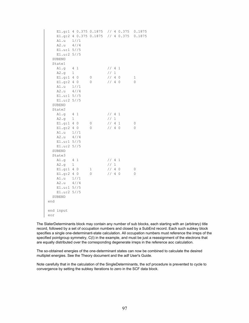
E1.g:1 4 0.375 0.1875 // 4 0.375 0.1875E1.g:2 4 0.375 0.1875 // 4 0.375 0.1875A1.u 1//1A2.u 4//4E1.u:1 5//5E1.u:2 5//5
SUBENDState1
A1.g 4 1 // 4 1A2.g 1 // 1E1.g:1 4 0 0 // 4 0 1E1.g:2 4 0 0 // 4 0 0A1.u 1//1A2.u 4//4E1.u:1 5//5E1.u:2 5//5
SUBENDState2
A1.g 4 1 // 4 1A2.g 1 // 1E1.g:1 4 0 0 // 4 1 0E1.g:2 4 0 0 // 4 0 0A1.u 1//1A2.u 4//4E1.u:1 5//5E1.u:2 5//5
SUBENDState3
A1.g 4 1 // 4 1A2.g 1 // 1E1.g:1 4 0 1 // 4 0 0E1.g:2 4 0 0 // 4 0 0A1.u 1//1A2.u 4//4E1.u:1 5//5E1.u:2 5//5
SUBENDend
end inputeor
The SlaterDeterminants block may contain any number of sub blocks, each starting with an (arbitrary) titlerecord, followed by a set of occupation numbers and closed by a SubEnd record. Each such subkey blockspecifies a single one-determinant-state calculation. All occupation numbers must reference the irreps of thespecified pointgroup symmetry, C(I) in the example, and must be just a reassignment of the electrons thatare equally distributed over the corresponding degenerate irreps in the reference aoc calculation.
The so-obtained energies of the one-determinant states can now be combined to calculate the desiredmultiplet energies. See the Theory document and the adf User's Guide.
Note carefully that in the calculation of the SingleDeterminants, the scf procedure is prevented to cycle toconvergence by setting the subkey Iterations to zero in the SCF data block.
97

CuH+: calculation of S2
Sample directory: adf/CuH+_S-squared/
Example calculates expectation value of S2 (< S2 >) of CuH+ in various symmetries, using unrestricteddensity functional theory. Last example in this example file calculates this value in the case there are morebeta electrons than alpha electrons.
$ADFBIN/adf << eorTitle calculate expectation value of S-squared
ATOMS Z-MatrixCu 0 0 0H 1 0 0 1.463
END
CHARGE 1.0 -1.0Unrestricted
FRAGMENTSH t21.HCu t21.CuEND
endinputeor
N2+: Localized Hole
Sample directory: adf/ModStPot_N2+/
This calculation illustrates:
• a) How to specify the net total charge on a molecule• b) How to enforce breaking the symmetry that is present in the start-up situation,
in this case to localize a hole in the electron density on one of the two equivalent atoms.• c) How to prevent the scf from oscillating back and forth between the two equivalent
situations or from even restoring the unwanted symmetry$ADFBIN/adf <<eortitle N2+ hole localization
atomsN 0 0 -2.0N 0 0 2.0end
BasisType DZPCore Small
End
98

symmetry C(lin) ! allow symmetry breaking
unrestricted
Occupations keeporbitals=3 &! keeporbitals: let the density relax a bit, then fix the MO occupssigma 3 // 1 0 1pi 2 // 2
end
CHARGE 1 1 ! this duplicates info from "OCCUPATIONS" (check)
modifystartpotential ! to break the symmetry in the start-up potentialN/1 0.5 0.5N/2 4 1end
end inputeor
The purpose of this run is to compute the N2+ ion, with the hole localized on one of the atoms. In a verysmall system like N2+ this is a tricky thing to do. The program has a tendency towards the symmetricsolution, with the hole delocalized. A few trial runs, just putting a net +1 charge into the system, will revealthat clearly.
To achieve the desired situation we apply the key modifystartpotential to break the symmetry of the initialpotential. A potential is generated as if the electronic cloud in the second N fragment is spin-polarized in aratio 4:1 (this precise value is not very relevant), which achieves that initially a non-symmetric solution isobtained. The symmetry must be specified, lest the program determine and use the higher symmetry fromthe nuclear frame. This would prevent any symmetry breaking altogether.
Next, in order to prevent that the system relaxes to the symmetric situation, we apply the keeporbitals optionof the occupations key. This fixes the occupied orbitals in the sense that in each scf cycle the program willtry to keep the electrons in orbitals that resemble the previously occupied orbitals as much as possible.
The key modifystartpotential here demonstrated has a more relevant and less unstable application in largersystems. See the User's Guide for references.
Fe4S4: broken spin-symmetry
Sample directory: adf/Fe4S4_BrokenSymm/
This calculation shows a spin-flip restart feature that allows to exchange alpha and beta fit coefficients forselected atoms upon restart. First the high spin configuration with 8 more α-electrons than beta-electrons iscalculated (Sz=4). Next the broken spin-symmetry configuration is calculated (Sz=0), using the subkeyspinflip in the restart key. In this case the spin will be flipped for iron atoms 1 and 2.
$ADFBIN/adf <<eorTITLE Fe4S4 High-spin configurationATOMSFe -0.000000000000 -1.256142548900 0.888226914500Fe 0.000000000000 1.256142548900 0.888226914500Fe -1.256142548900 0.000000000000 -0.888226914500Fe 1.256142548900 -0.000000000000 -0.888226914500
99

S -1.845393493800 0.000000000000 1.304890253400S 1.845393493800 -0.000000000000 1.304890253400S -0.000000000000 -1.845393493800 -1.304890253400S 0.000000000000 1.845393493800 -1.304890253400
END
Symmetry C(2v)
CHARGE 0.0 8.0UNRESTRICTED
BASIStype DZcore Largecreateoutput NoneEND
XCGGA OPBEENDend inputeor
mv TAPE21 Fe4S4-high-spin.t21
$ADFBIN/adf <<eorTITLE Fe4S4 LOW-spin configuration
Restart Fe4S4-high-spin.t21 &! Make sure atoms specified in the SpinFlip keyword aresymmetry-equivalent
SpinFlip 1 2End
ATOMSFe -0.000000000000 -1.256142548900 0.888226914500Fe 0.000000000000 1.256142548900 0.888226914500Fe -1.256142548900 0.000000000000 -0.888226914500Fe 1.256142548900 -0.000000000000 -0.888226914500S -1.845393493800 0.000000000000 1.304890253400S 1.845393493800 -0.000000000000 1.304890253400S -0.000000000000 -1.845393493800 -1.304890253400S 0.000000000000 1.845393493800 -1.304890253400
END
Symmetry C(2v)
CHARGE 0.0 0.0
UNRESTRICTED
BASIStype DZcore Largecreateoutput NoneEND
100
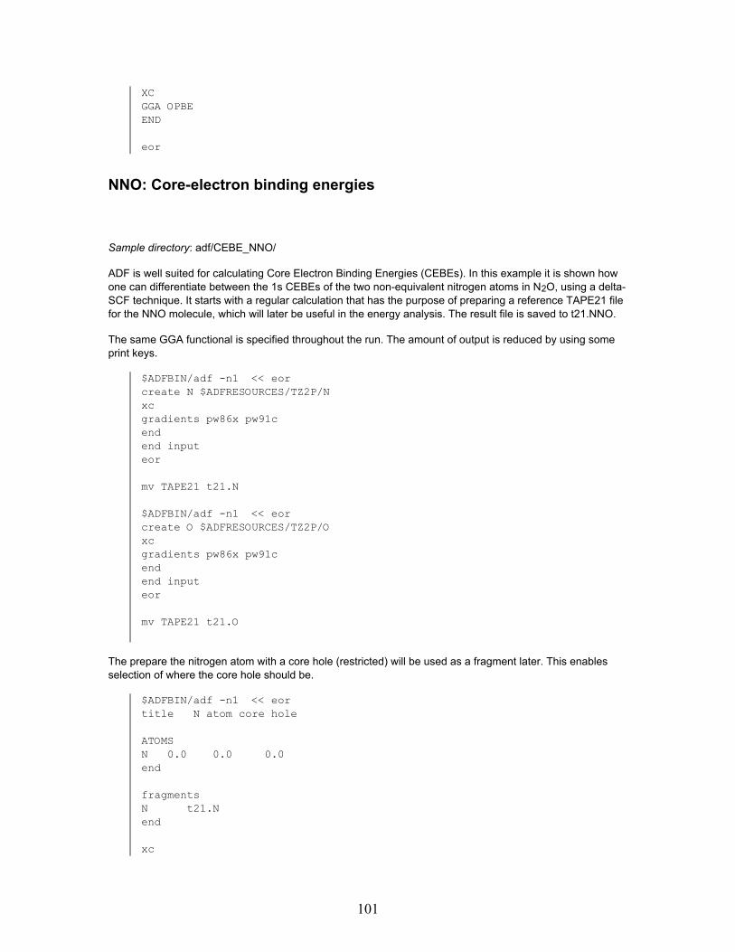
XCGGA OPBEEND
eor
NNO: Core-electron binding energies
Sample directory: adf/CEBE_NNO/
ADF is well suited for calculating Core Electron Binding Energies (CEBEs). In this example it is shown howone can differentiate between the 1s CEBEs of the two non-equivalent nitrogen atoms in N2O, using a delta-SCF technique. It starts with a regular calculation that has the purpose of preparing a reference TAPE21 filefor the NNO molecule, which will later be useful in the energy analysis. The result file is saved to t21.NNO.
The same GGA functional is specified throughout the run. The amount of output is reduced by using someprint keys.
$ADFBIN/adf -n1 << eorcreate N $ADFRESOURCES/TZ2P/Nxcgradients pw86x pw91cendend inputeor
mv TAPE21 t21.N
$ADFBIN/adf -n1 << eorcreate O $ADFRESOURCES/TZ2P/Oxcgradients pw86x pw91cendend inputeor
mv TAPE21 t21.O
The prepare the nitrogen atom with a core hole (restricted) will be used as a fragment later. This enablesselection of where the core hole should be.
$ADFBIN/adf -n1 << eortitle N atom core hole
ATOMSN 0.0 0.0 0.0end
fragmentsN t21.Nend
xc
101

gradients pw86x pw91cend
eprintSFO noeig noovlend
occupationss 1 2p 3end
end inputeor
mv TAPE21 t21.N_ch
Now perform the restricted ground state molecule for analysis later. The TAPE21 result file is saved.
$ADFBIN/adf << eortitle NNO
noprint sfofragpop fragsfo
xcgradients pw86x pw91cend
ATOMSN 0.0 0.0 -1.1284N 0.0 0.0 0.0O 0.0 0.0 1.1841end
fragmentsN t21.NO t21.Oend
eprintSFO noeig noovlend
end inputeor
mv TAPE21 t21.NNO
Next follow two sets of almost identical calculations in which a 1s electron is removed from one or the otherN atom (please note that the deepest s level is associated with the 1s of the oxygen atom). The molecularNNO result file is used as fragment. An unrestricted calculation is done and a positive charge is specified.The final result file for the molecule with the core hole is saved. Then another calculation is done toconveniently obtain the energy with respect to the normal molecule. This is repeated for a core hole on theother N atom.
$ADFBIN/adf <<eor
102

title NNO unrestricted core hole
noprint sfofragpop fragsfo
ATOMSN 0.0 0.0 -1.1284 f=N_chN 0.0 0.0 0.0 f=NO 0.0 0.0 1.1841 f=Oend
xcgradients pw86x pw91cend
fragmentsN_ch t21.N_chN t21.NO t21.Oend
eprintSFO noeig noovlend
unrestrictedcharge 1 1
occupationsigma 1 1 1 4 // 1 0 1 4pi 4 // 4end
end inputeor
mv TAPE21 t21.NNO.unr1
In the second calculation the result file of one of the unrestricted NNO calculations is used as restart file,which ensures that the hole stays at its place, because the starting density is already correct. The result filet21.NNO for the normal NNO calculation is specified as fragment to serve as an energy reference. The finalBonding Energy printed by ADF indicates what the CEBE is. However, please check Refs.[Chong, 2002#1239][Chong, 2002 #1238] for more detailed information on Core-Electron Binding Energies. Thesereferences also contain infomration on empirical corrections that may have to be made on the final numbers.
$ADFBIN/adf <<eortitle NNO unr. core hole
noprint sfofragpop fragsfo
xcgradients pw86x pw91cend
restart t21.NNO.unr1
ATOMSN 0.0 0.0 -1.1284 f=NNO
103

N 0.0 0.0 0.0 f=NNOO 0.0 0.0 1.1841 f=NNOend
eprintSFO noeig noovlend
fragmentsNNO t21.NNOend
unrestrictedcharge 1 1
occupationsigma 1 1 1 4 // 1 0 1 4pi 4 // 4
end
end inputeor
Similarly, one could easily have prepared an oxygen with a core hole and determined the CEBE of theoxygen 1s atom.
104

Spectroscopic Properties
IR Frequencies, (resonance) Raman, VROA, VCD, Franck-Condon factors
NH3: Numerical Frequencies
Sample directory: adf/Freq_NH3/
Summary:
• Frequencies with symmetric displacements• Frequencies with Cartesian displacements• Isotope effects in the frequencies
Frequencies with symmetric displacements
Computation of frequencies by symmetric displacements. The assumed equilibrium input structure shouldbe given in Cartesian coordinates.
The symmetry is determined automatically by the program as C(3v), from the input coordinates. During thecalculation first symmetric atomic displacements are constructed. The number of such displacements ineach irreducible representation corresponds to the number of frequencies with the corresponding symmetry.All displaced geometries within one representation have the same symmetry, which enables us to use it tospeed up the computation significantly. Another advantage of having the same symmetry is that thenumerical integration data can be reused efficiently (see SMOOTH option) thus reducing the level ofnumerical noise in gradients and force constant matrix.
$ADFBIN/adf <<eortitle NH3 frequencies in symmetric displacements
atomsN 0.0000 0.0000 0.0000H 0.4729 0.8190 0.3821H -0.9457 0.0000 0.3821H 0.4729 -0.8190 0.3821
end
BasisType TZPCore Small
End
geometryfrequencies Symm
end
thermo T=300,400
integration 5.0
105

end inputeor
Frequencies with Cartesian displacements
Computation of frequencies by Cartesian displacements. The assumed equilibrium input structure is given ininternal coordinates. A dummy atom is used for a convenient definition of the Z-matrix such that it reflectsthe pointgroup symmetry C(3v).
$ADFBIN/adf <<eortitle NH3 frequencies
definerNH=1.02theta=112phi=120
end
atoms Z-matrixXX 0 0 0N 1 0 0 1.0H 2 1 0 rNH thetaH 2 1 3 rNH theta phiH 2 1 4 rNH theta phi
end
BasisType TZPCore Small
End
geometryoptim cartesianfrequencies
end
thermo T=300,400
integration 5.0
end inputeor
The symmetry is determined automatically by the program as C(3v), from the input coordinates. In aFrequencies calculation the symmetry (specified on input or computed internally) is used for analysis and insome cases to speed up the calculation.
The equilibrium coordinate values are supplied as identifiers that are associated with values in the defineblock.
Unlike using the geovar key, applying the define key does not mean anything in the sense that the variouscoordinates that refer to the same identifier would be forced to remain equal; it is just a way to display (to thehuman reader) symmetry in the equilibrium values, to avoid typing errors and to allow an easy adjustment ofstarting coordinates for another calculation.
106

Since the atomic coordinates are input in Z-matrix format, the program would by default carry outdisplacements in internal coordinates to scan the energy surface and hence compute force constants andfrequencies. This is overriden by specifying in the geometry block optim cartesian: carry out cartesiandisplacements.
The key thermo addresses the thermodynamical analysis (only available in a Frequencies calculation,otherwise ignored). The specification 'T=300,400' means that the thermodynamic properties are printed forthe temperature range 300-400K, in steps of 10K (default) and for a pressure of 1.0 atmosphere (default).
Frequencies calculations suffer easily from numerical inaccuracies. Therefore, the default numericalintegration precision in a Frequencies calculation is much higher than in an ordinary single-point orminimization run. Here we specify the INTEGRATION level to be 5.0 (quite high, but the default forFrequencies is even 6.0).
Isotope effects in the frequencies
Rename the TAPE21 result file of the previous calculation so we can restart with other masses. Calculate adifferent isotope of H, in this case deuterium. It will differ from the original one only in the mass of thenucleus. Repeat the frequency calculation with different fragments. It is important to preserve symmetry atthis step so we replace fragment files for ALL H atoms. If you want to replace only one fragment then theoriginal calculation must be performed the same way, with different fragment names.
mv TAPE21 restart.t21
$ADFBIN/adf -n1 <<eorcreate H M=2.014101779 $ADFRESOURCES/TZP/Heor
mv TAPE21 t21.D
$ADFBIN/adf <<eortitle NH3 frequencies
definerNH=1.02theta=112phi=120
end
atoms Z-matrixXX 0 0 0N 1 0 0 1.0H 2 1 0 rNH thetaH 2 1 3 rNH theta phiH 2 1 4 rNH theta phi
end
FragmentsN t21.N
! The different isotope mass sits in the next line.H t21.D
End
geometryoptim cartesianfrequencies
107

end
! Restart the frequency calculation.! In fact ADF should perform only one geometry cyclerestart restart.t21
thermo T=300,400
integration 5.0
end inputeor
UF6: Numerical Frequencies, spin-orbit coupled ZORA
Sample directory: adf/Freq_UF6/
Calculation of spin-orbit coupled ZORA gradients for the LDA and GGA functionals is possible since theADF2007.01 version.Summary:
• Geometry optimization• Frequencies with symmetric displacements• Both for scalar relativistic ZORA and spin-orbit coupled ZORA
Geometry optimization
Here only the spin-orbit coupled input file for ADF is given (in the scalar relativistic case change "spinorbit" in"scalar"). The resulting TAPE21 is saved such that it can be used in the frequency calculation.
$ADFBIN/adf <<eorTitle UF6 geometry optimization: scalar ZORAintegration 5 5Geometryconv grad=1e-4
Endrelativistic spinorbit zoraBasisType TZP
endATOMS cartesian1 U .00000 .00000 .000002 F 2.00000 .00000 .000003 F -2.00000 .00000 .000004 F .00000 2.0000 .000005 F .00000 -2.0000 .000006 F .00000 .0000 2.000007 F .00000 .0000 -2.00000ENDend inputeormv TAPE21 UF6.t21
108

Frequencies with symmetric displacements
Computation of frequencies by symmetric displacements. The assumed equilibrium input structure shouldbe given in Cartesian coordinates. The calculation starts with the optimized structure read from UF6.t21(restart file). Again only the spin-orbit coupled input file for ADF is given.
The symmetry is determined automatically by the program as O(H), from the input coordinates. During thecalculation first symmetric atomic displacements are constructed. The number of such displacements ineach irreducible representation corresponds to the number of frequencies with the corresponding symmetry.All displaced geometries within one representation have the same symmetry, which enables us to use it tospeed up the computation significantly. Another advantage of having the same symmetry is that thenumerical integration data can be reused efficiently (see SMOOTH option) thus reducing the level ofnumerical noise in gradients and force constant matrix.
In case of spin-orbit coupling the frequencies can not (yet) be calculated with analytical second derivatives.
$ADFBIN/adf <<eorTitle UF6 frequencies and IR intensities: spinorbit ZORARestart UF6.t21Geometry
Frequencies SymmEndintegration 5 5relativistic spinorbit zoraFragmentsU t21.UF t21.F
endATOMS cartesian1 U .00000 .00000 .000002 F 2.00000 .00000 .000003 F -2.00000 .00000 .000004 F .00000 2.0000 .000005 F .00000 -2.0000 .000006 F .00000 .0000 2.000007 F .00000 .0000 -2.00000ENDend inputeor
H2O: Numerical Frequencies, accurate Hartree-Fock
Sample directory: adf/H2O_HF_freq/
Example shows a Hartree-Fock frequency calculation with an accurate basis set.
The 'DEPENDENCY' key is set to 1e-4. Note that for hybrids and Hartree-Fock the dependency key isalways set. The default value in that case is 4e-3. By explicitely setting the 'DEPENDENCY' key we can usea lower value, which is possible in this case. One should check that the results remain reliable if one uses asmaller value for the 'DEPENDENCY' key.
First a geometry optimization is performed.
109

$ADFBIN/adf << eortitle accurate HF geometry optimization with large QZ4P basis setbasistype QZ4Pcore None
endadddiffusefitdependency bas=1e-4ATOMS
O 0.000000 0.000000 -0.007124H 0.000000 0.751933 0.556531H 0.000000 -0.751933 0.556531
ENDintegration 6 6 6xchartreefock
endgeometryendend inputeormv TAPE21 t21
Next the frequency calculation is done. A restart is used to pick up the excited state geometry of theprevious calculation. The orbitals are not read from the restart file (subkey NoOrb in the restart key). Alsothe fit coefficients are not read from the restart file (subkey NoSCF in the restart key).
$ADFBIN/adf << eortitle accurate HF frequency calculation with large QZ4P basis setrestart t21 &noscfnoorb
endbasistype QZ4Pcore None
endadddiffusefitdependency bas=1e-4ATOMS
O 0.000000 0.000000 -0.007124H 0.000000 0.751933 0.556531H 0.000000 -0.751933 0.556531
ENDintegration 6 6 6xchartreefock
endgeometryfrequencies symm
endend inputeor
110

PH2: Numerical Frequencies of an excited state
Sample directory: adf/EGO_PH2/
Example for an excited state geometry optimization and frequency calculation.
Needed for such excited state optimizations are the key EXCITATIONS (to calculate excitation energies),the key GEOMETRY (to do a geometry optimization) and the key EXCITEDGO (to select for whichexcitation a geometryy optimization should be performed). The ground state and excited state are openshell.
$ADFBIN/adf <<eorTITLE PH2 Excited state geometryatoms
P 0.000000 0.000000 0.0H 0.7 0.0 0.7H -0.7 0.0 0.7
endXCGGA BP86
ENDUNRESTRICTEDCHARGE 0 1Integration 6.0 6.0 6.0GEOMETRYITERATIONS 50CONVERGENCE E=0.0001 grad=0.00001
ENDSCF
converge 1.0e-9ENDbasisTYPE DZCORE NONE
endexcitationsLOWEST 10onlysingletendEXCITEDGOSTATE B2 1OUTPUT=1
endeormv TAPE21 PH2.t21
Next the frequencies are calculated of the excited state. A restart is used to pick up the excited stategeometry of the previous calculation. Note that in a numerical FREQUENCIES calculation symmetry isturned off except to reduce the number of points calculated. Thus irrespective of the specified point groupsymmetry the symmetry label A of SYMMETRY NOSYM should be used to select the excited state. Careshould be taken to ensure that the correct state is chosen in this frequencies calculation as the excited statenumber can change when the point group is changed. In this case instead of 'B2 1' one needs to select 'A 1'.Accurate SCF convergence parameters are used.
111

$ADFBIN/adf <<eorTITLE PH2 Excited state frequenciesatomsP 0.000000 0.000000 0.002878H 1.258230 0.000000 0.655775H -1.258230 0.000000 0.655775endXCGGA BP86
ENDUNRESTRICTEDCHARGE 0 1Integration 6.0GEOMETRYFREQUENCIES
ENDSCF
converge 1.0e-9ENDbasisTYPE DZ
CORE NONEendexcitationsLOWEST 10onlysingletendEXCITEDGOSTATE A 1OUTPUT=2CPKS EPS=0.000001
endeor
CN: Analytic Frequencies
Sample directory: adf/CN_SecDeriv/
The ADF2002.01 version featured analytic second derivatives (SD) for the first time. This initialimplementation had severe limitations, both in terms of speed, as in terms of user-friendliness of the outputand the number of available options. As of ADF2006.01, the implementation has been significantlyimproved. More specifically:
• what was formerly a separate SD program is now part of the main ADF executable;• most current GGA's have been implemented, with the exeption of PW91;• the speed of the code, serial as well as parallel, has been improved;• full support for symmetry has been implemented, including linear molecules.
Calculation of analytical second derivatives is requested by specifying
AnalyticalFreqEnd
in the main ADF input.
112

A high accuracy is specified for the numerical integration to be sure of reliable results.i In general, it seemsadvisable to use high accuracy for heavy nuclei at the moment, whereas default integration accuracy isusually sufficient for light atoms. Further, high integration accuracy is more needed in the atomic spheresthan in the rest of the molecule. A cost-effective solution may therefore be to specify a higher integrationaccuracy in the spheres only (using the accsph subkey of the INTEGRATION keyword).
$ADFBIN/adf << eortitle CN
atomsN -1.3 0.0 0.0C 0.0 0.0 0.0
end
BasisType DZCore None
End
charge -1
XCLDA Xonly
End
integration 6.0
AnalyticalFreqEnd
End inputeor
After SCF is completed, the energy second derivatives matrix is calculated and analysed, which yields in thiscase one frequency.
CH4: Analytic Frequencies
Sample directory: adf/CH4_SecDeriv/
In this example, we use a new feature of adf2006.01: geometry optimization immediately followed bycalculation of frequencies. This is done by specifying the Geometry and AnalyticalFreq input blocks in onefile.
Note: when using this feature, one should generally set the integration accuracy to a value appropriate forthe frequencies calculation, which is about 5.0. In order to save time we neglect the recommendation in thisexample.
$ADFBIN/adf << eortitle CH4 LDA potential
DefineZERO = 0.0RCH = 1.0850
113

DCH = sqrt(3)*(RCH/3)End
AtomsC 0.0 0.0 0.0H DCH -DCH DCHH DCH DCH -DCHH -DCH DCH DCHH -DCH -DCH -DCH
End
BasisType TZPCore None
End
integration 4.0
GeometryOptim allconverge grad=0.0001
End
AnalyticalFreqEnd
End inputeor
HI: Analytic Frequencies, scalar ZORA
Sample directory: adf/HI_SecDer_ZORA/
The main difference of this example to the previous examples is that a ZORA Hessian is calculated in thisexample, through the line:
RELATIVISTIC scalar ZORA
Furthermore, the suggestion to use high integration accuracy in the atomic spheres only is shown explicitlyhere.
$ADFBIN/adf << eorTITLE HI scalar, ZORA,DEFINEZERO = 0.0R = 1.6090X1 = ZEROY1 = ZEROZ1 = RX2 = ZEROY2 = ZEROZ2 = ZERO
ENDATOMS
114

I X2 Y2 Z2H X1 Y1 Z1
ENDXCLDA Xonly
ENDRELATIVISTIC scalar ZORACOREPOTENTIALS t12.rel &H 1I 2
ENDFRAGMENTSH t21HI t21I
ENDintegration
accint 4.0accsph 6.0
end
AnalyticalFreqEnd
end inputeor
Ethanol: mobile block Hessian
Sample directory: adf/MBH_Ethanol/
A frequency calculation is performed using the mobile block Hessian (MBH) method. The coordinates in theATOMS section should be the partially optimized coordinates (or the fully optimized coordinates would worktoo). The next input for ADF shows how to perform a frequency calculation with MBH. The flag b=b1 in theATOMS section adds the label 'b1' to some of the atoms. Only the four atoms labeled 'b1' (CH3) will beconsidered as a block with fixed internal geometry.
$ADFBIN/adf <<eorTITLE ethanol: second derivatives with MBH approach. CH3 is treated as arigid block
ATOMS1 C -0.029587 -0.006554 0.008124 b=b12 H -0.087498 -0.025163 1.109913 b=b13 H 1.027473 -0.056237 -0.302751 b=b14 H -0.565305 -0.891154 -0.376242 b=b15 C -0.694908 1.238909 -0.501807 b=b26 H -0.670258 1.265092 -1.608847 b=b27 O -2.069894 1.175059 -0.0172518 H -0.182335 2.138977 -0.109315 b=b29 H -2.586972 1.972802 -0.317216END
SYMMETRY nosym
115

BASIStype DZcore LargeCreateOutput None
END
XCLDA SCF VWNEND
GEOMETRYfrequenciesmbh b1branch new
END
INTEGRATION 6.0End inputeor
For comparison in this example also a calculation is performed without any restrictions.
$ADFBIN/adf <<eorTITLE ethanol: complete vibrational spectrum, compare with MBH above
ATOMS1 C -0.029587 -0.006554 0.0081242 H -0.087498 -0.025163 1.1099133 H 1.027473 -0.056237 -0.3027514 H -0.565305 -0.891154 -0.3762425 C -0.694908 1.238909 -0.5018076 H -0.670258 1.265092 -1.6088477 O -2.069894 1.175059 -0.0172518 H -0.182335 2.138977 -0.1093159 H -2.586972 1.972802 -0.317216END
BASIStype DZcore LargeCreateOutput None
END
XCLDA SCF VWNEND
AnalyticalFreqEnd
INTEGRATION 5.0End inputeor
116

CH4: mobile block Hessian
Sample directory: adf/MBH_CH4/
A frequency calculation is performed using the mobile block Hessian (MBH)method. The coordinates in theATOMS section should be the partially optimized coordinates (or the fully optimized coordinates would worktoo).
Example input how to do a block constraint:
ATOMSC 0.000000 0.000000 0.000000 b=b1H 0.634671 0.634671 0.634671 b=b1H -0.634671 -0.634671 0.634671 b=b1H -0.634671 0.634671 -0.634671 b=b1H 0.634671 -0.634671 -0.634671
ENDCONSTRAINTSblock b1
END
Such geometry optimization will not be discussed here any further. The next input for ADF shows how toperform a frequency calculation with MBH.
$ADFBIN/adf <<eorTITLE Methane
BASISType DZCore None
END
ATOMSC 0.000000 0.000000 0.000000 b=b1H 0.634671 0.634671 0.634671 b=b1H -0.634671 -0.634671 0.634671 b=b1H -0.634671 0.634671 -0.634671 b=b1H 0.634671 -0.634671 -0.634671 b=b2
END
integration 8 8 8SYMMETRY nosym
GEOMETRYfrequencies disrad=0.001mbh b1branch new
ENDEnd inputeor
The flag b=b1 in the ATOMS section adds the label 'b1' to some of the atoms. The four atoms labeled 'b1'will be considered as a block with fixed internal geometry.
117

In the GEOMETRY section, a Mobile Block Hessian calculation is requested by using the FREQUENCIESand MBH keywords. Here the atoms with label 'b1' are selected to be in the same mobile block. Theposition/orientation of the block are supposed to be optimized in a preceding partial optimization run. In thevibrational analyis, the block 'b1' is only allowed to vibrate as a whole. The number of resulting modes/frequencies is 3 for the fifth atom plus 6 for the block 'b1' (3 position/3 orientation), resulting in 9 frequenciesin total. Since 6 of those frequencies are zero due to translational and rotational invariance of the system,one will find 3 non-zero characteristic frequencies in the output. In practice with ADF not exactly 6 zero's arefound, but they are close to zero.
The quality of the frequencies/modes depends largely on the block choice. Best results are obtained whengrouping atoms in a block if those atoms are known to form rather rigid structures. For instance, groupingthe 11 atoms of benzene side group into a block, will usually result in representative frequencies. In thisexample the block choice is only illustrative for the methodology.
NH3: Raman
Sample directory: adf/Freq_NH3_RAMAN/
Summary:
• Analytical frequencies with subsequent calculation of Raman intensities in a range• Numerical frequencies including all Raman intensities
Raman Intensities for Selected Frequencies
The RamanRange keyword (available since ADF2007.01) can be used to calculate Raman intensities for arange of frequencies only. Using this option is a fast alternative for the existing method of calculating Ramanintensities, which is described in the second part of this example.
Two values defining an interval of frequencies to calculate the Raman intensities for. The Raman intensitiesare calculated by numerical differentiation of the polatizability tensor. Only frequencies frequencies withingthe interval that are known to be Raman-active will be included.
$ADFBIN/adf <<eortitle NH3 frequencies and calculation of Raman intensities in the range0-2000 cm-1atoms
N 0.0000 0.0000 0.0000H 0.4729 0.8190 0.3821H -0.9457 0.0000 0.3821H 0.4729 -0.8190 0.3821
endBasisType TZPCore Small
EndAnalyticalFreqendthermo T=300,400integration 5.0end inputeor
118

mv TAPE21 NH3_freqs.t21
$ADFBIN/adf <<eortitle NH3 Raman intensities in the range 0-2000 cm-1atoms
N 0.0000 0.0000 0.0000H 0.4729 0.8190 0.3821H -0.9457 0.0000 0.3821H 0.4729 -0.8190 0.3821
endRestart NH3_freqs.t21FragmentsH t21.HN t21.N
EndRamanRange 0.0 2000.0thermo T=300,400integration 5.0end inputeor
Raman Intensities for All Frequencies
Raman scattering intensities and depolarization ratios for all molecular vibrations at a certain laser frequencycan be calculated in a single run. The run type must be Frequencies and the RESPONSE key is used tospecify that Raman intensities are computed.
In this example the static Raman scattering is calculated (ω = 0). This type of calculation is very similar to anIR intensity calculation. In fact, all IR output is automatically generated as well. At all distorted geometriesthe dipole polarizability tensor is calculated. This is very time-consuming and is only feasible for smallmolecules.
$ADFBIN/adf <<eortitle NH3 frequencies with Raman intensitiesatoms
N 0.0000 0.0000 0.0000H 0.4729 0.8190 0.3821H -0.9457 0.0000 0.3821H 0.4729 -0.8190 0.3821
endFragmentsH t21.HN t21.N
Endgeometry
frequenciesendresponse
ramanendthermo T=300,400integration 5.0end inputeor
119

HF: Resonance Raman, excited state finite lifetime
Sample directory: adf/HF_ResonanceRaman/
Example shows a calculation of the Resonance Raman spectrum (RRS) of HF. In this example the RRS iscalculated from the geometrical derivatives of the frequency-dependent polarizability, including a finitelifetime.
In the ADF input one then needs to include the subkey FREQUENCIES of the key GEOMETRY (numericalfrequencies) and include the subkeys RAMAN and LIFETIME of the key AORESPONSE.
$ADFBIN/adf << eortitle HF ao-raman
BASISF DZP/FH DZP/H
END
GEOMETRYFrequencies
END
Symmetry NOSYM
AtomsH 0.0000 0.0000 0.0000F 0.0000 0.0000 0.9170
End
aoresponsefrequency 1 0.52362 Hartreelifetime 0.0034raman
end
NOPRINT SFO
END INPUTeor
Note that used basis set is too small to get accurate results.
Uracil: Resonance Raman, excited state gradient
Sample directory: adf/Vibron_RR_uracil/
Example shows a calculation of the Resonance Raman spectrum (RRS) of uracil. In this example the RRSis calculated using the excited-state gradient.
120

A frequency restart file 'restart.freq' is used as input in the resonance Raman calculation. This restart file isthe TAPE21 of a frequency calculation of the runfile 'restart.freq.run'.
First the to ASCII dumped TAPE21 'restart.freq.ascii' is undumped again to make a binary file.
cp $ADFHOME/examples/Test/e_Vibron_RR_uracil/restart.freq.ascii .$ADFBIN/udmpkf < restart.freq.ascii restart.freq
Next the resonance Raman calculation is performed by setting the 'VIBRON' subkey in the 'GEOMETRY'block key, including both the 'EXCITATION' block key and the 'VIBRON' block key. These are the onlydifferences with the frequency run where only the 'FREQUENCIES' subkey was set in the 'GEOMETRY'block key., and the 'EXCITATION' and 'VIBRON' block key were not set.
$ADFBIN/adf << eorTitle Input generated by modcoEPRINT
SFO NOEIG NOOVL NOORBPOPSCF NOPOP
ENDNOPRINT BAS FUNCTIONSUNITS
length angstromangle degree
ENDATOMS
N -0.0147481688 -0.0251586720 0.0000000000C -0.0263429706 1.3809974655 0.0000000000N 1.2556533768 1.9305098959 0.0000000000C 2.5041083561 1.2440596334 0.0000000000C 2.3755611578 -0.2074475201 0.0000000000C 1.1446314693 -0.7882184482 0.0000000000H -0.9346804118 -0.4675883900 0.0000000000O -1.0845317554 2.0515533614 0.0000000000H 1.3029888073 2.9549419374 0.0000000000O 3.5819185026 1.8899458170 0.0000000000H 3.2859343437 -0.7987226158 0.0000000000H 0.9976482662 -1.8650665505 0.0000000000
ENDBASIS
type DZcore NONE
ENDXC
GGA Becke88 Perdew86ENDSYMMETRY tol=0.001GEOMETRY
VIBRONENDSCF
iterations 50converge 1.0e-6 1.0e-6mixing 0.2lshift 0.0diis n=10 ok=0.5 cyc=5 cx=5.0 cxx=10.0
ENDEXCITATION
ONLYSING
121

LOWEST 5ENDMBLOCKBIGVIBRON
NMTAPE restart.freqRESRAMANSTPSIZ 0.1DOMODES 11 13 16 17DSCHEME ELCHAR
ENDINTEGRATION 4.0 4.0END INPUT
Note that used basis set is too small to get accurate results.
H2O2: vibrational Raman optical activity (VROA)
Sample directory: adf/VROA/
Example shows a calculation of normal vibrational Raman optical activity.
In the ADF input one then needs to include the subkey FREQUENCIES of the key GEOMETRY (numericalfrequencies) and include the subkey VROA of the key AORESPONSE. A laser frequency need to be added.The other keys in AORESPONSE are recommende by the author of the implementation of VROA in ADF.For accuracy reasons 'INTEGRATION 6' and EXACTDENSITY are used.
$ADFBIN/adf << eortitle VROA TEST H2O2
basistype TZPcore None
end
ATOMS1.O -0.750254 -0.034490 0.0151332.O 0.750254 0.034490 0.0151333.H -0.943532 0.744006 0.5800404.H 0.943532 -0.744006 0.580040
END
xcgga BLYP
end
GEOMETRYfrequenciesENDexactdensity
INTEGRATION 6.0 6.0 6.0
aoresponseNEWPOLCODE
122

VROAscf converge 1d-6 iterations 100frequency 1 5145 AngstromALDAFitAOderivEL_DIPOLE_EL_DIPOLE VELOCITYEL_DIPOLE_EL_QUADRUPOLE VELOCITYEL_DIPOLE_MAG_DIPOLE VELOCITY
end
END INPUTeor
Note that used basis set is too small to get accurate results. Better is the use larger basis sets, like one ofthe even tempered basis sets (for example Type ET/ET-QZ3P-1DIFFUSE), or use augmented basis sets(for example Type AUG/ATZ2P).
H2O2: resonance VROA
Sample directory: adf/VROA_RESO/
Example shows a calculation of resonance vibrational Raman optical activity (resonance VROA).
In the ADF input one then needs to include the subkey FREQUENCIES of the key GEOMETRY (numericalfrequencies) and include the subkeys VROA and LIFETIME of the key AORESPONSE. A laser frequencyneed to be added. The other keys in AORESPONSE are recommende by the author of the implementationof VROA in ADF. For accuracy reasons 'INTEGRATION 6' and EXACTDENSITY are used.
$ADFBIN/adf << eortitle VROA TEST H2O2
basistype TZPcore None
end
ATOMS1.O -0.750254 -0.034490 0.0151332.O 0.750254 0.034490 0.0151333.H -0.943532 0.744006 0.5800404.H 0.943532 -0.744006 0.580040
END
xcgga BLYP
end
GEOMETRYfrequenciesENDexactdensity
INTEGRATION 6.0 6.0 6.0
123

aoresponseNEWPOLCODEVROAscf converge 1d-6 iterations 100frequency 1 5.15462 eVlifetime 0.0037ALDAFitAOderivEL_DIPOLE_EL_DIPOLE VELOCITYEL_DIPOLE_EL_QUADRUPOLE VELOCITYEL_DIPOLE_MAG_DIPOLE VELOCITY
end
END INPUTeor
Note that used basis set is too small to get accurate results. Better is the use larger basis sets, like one ofthe even tempered basis sets (for example Type ET/ET-QZ3P-1DIFFUSE), or use augmented basis sets(for example Type AUG/ATZ2P).
NHDT: Vibrational Circular Dichroism
Sample directory: adf/VCD_COG_NHDT/
Analytical frequencies with subsequent calculation of vibrational circular dichroism (VCD)
The VCD keyword (available since ADF2007.01) can be used to calculate VCD spectra. It is important tonote that the VCD keyword only works in combination with the keys AnalyticalFreq and symmetry NOSYM.
Recomended is use to use high accuracy for the geometry optimization which one needs to do before thefrequency calculation. This simple example is an NHDT molecule, which is NH3 where one hydrogen atom isreplaced with deuterium and another with tritium.
First the atoms are created, next the molecule is calculated.
$ADFBIN/adf -n1 <<eorcreate H q=1 m=2.014101778 file=$ADFRESOURCES/TZP/HXCgga Becke Perdew
endend inputeormv TAPE21 t21.D
$ADFBIN/adf -n1 <<eorcreate H q=1 m=3.01604927 file=$ADFRESOURCES/TZP/HXCgga Becke Perdew
endend inputeormv TAPE21 t21.T
$ADFBIN/adf -n1 <<eor
124

create N file=$ADFRESOURCES/TZP/NXCgga Becke Perdew
endend inputeormv TAPE21 t21.H
$ADFBIN/adf -n1 <<eorcreate N file=$ADFRESOURCES/TZP/NXCgga Becke Perdew
endend inputeormv TAPE21 t21.N
Next the molecule is calculated.
$ADFBIN/adf <<eorTitle Single Point calc.
AtomsN 0.000000 0.000000 0.010272H -0.471582 -0.816803 0.407861H.D 0.943163 0.000000 0.407861H.T -0.471582 0.816803 0.407861
End
Symmetry NOSYM
xcGGA BP86
end
FragmentsN t21.NH t21.HH.D t21.DH.T t21.TEnd
Integration 7.0
AnalyticalFreqEnd
VCD
end inputeor
NO2: Franck-Condon Factors
125

Sample directory: adf/FranckCondon_NO2/
As an example of a Franck-Condon calculation, lets look at the transition of NO2 to NO2-. NO2 is a smallmolecule with only three vibrational modes. Putting an extra electron on the molecule will cause a bigdisplacement, resulting in large electron-phonon couplings.
In general, the larger the molecule, the smaller the displacement and hence the electron-phonon couplingsand Franck-Condon factors. Moreover, larger molecules have more vibrational modes, meaning that thealready smaller displacement will generally be smeared out over more modes, resulting in an additionaldecrease in electron-phonon couplings. This is fortunate, since the number of Franck-Condon factorsincreases factorially with the number of vibrational modes, making it prohibitively expensive to take morethan a few vibrational quanta into account for most molecules.
In order to calculate the Franck-Condon factors for Nitrite and Nitrogen dioxide, the equilibrium positions ofthe nuclei and the vibrational modes have to be obtained (the geometry optimizations are not shown here):
$ADFBIN/adf << eor
TITLE Nitrogen dioxide
ATOMSN 0.000000 0.000000 -0.016179O 0.000000 1.098646 -0.492918O 0.000000 -1.098646 -0.492918
END
BASISCORE NONETYPE DZP
END
XCLDA SCF VWN
END
ANALYTICALFREQEND
eor
mv TAPE21 NO2.t21rm t21.* logfile
$ADFBIN/adf << eor
TITLE Nitrite
ATOMSN 0.000000 0.000000 0.093662O 0.000000 1.120366 -0.540999O 0.000000 -1.120366 -0.540999
END
CHARGE -1.0 1.0UNRESTRICTED
BASISCORE NONE
126

TYPE DZPEND
XCLDA SCF VWN
END
ANALYTICALFREQEND
eor
mv TAPE21 NO2-.t21rm t21.* logfile
This runscript produces two TAPE21 files containing the frequencies and the normal modes for both chargestates. Lets first look at the ground state to ground state overlap:
$ADFBIN/fcf << eor
STATES NO2.t21 NO2-.t21
QUANTA 0 0
TRANSLATEROTATE
eor
Here, zero vibrational quanta are specified for both charge states, which corresponds to the vibrationalground state. Looking at the standard output, we see for NO2:
Frequency (cm-1) λ (dimensionless)1072.490460 1.2161081434.990571 1.8739151875.876562 0.000000
And for NO2-:
Frequency (cm-1) λ (dimensionless)816.952242 0.5946431264.390562 2.0713191314.362101 0.000000
Both states have two vibrational modes with a significant electron-phonon coupling. The ground state toground state Franck-Condon factor is therefore expected to be quite small. And indeed, looking at theoutput, we see that it is 0.7944250686*10-2, less than one percent of the total.
Since NO2 has only three vibrational modes, many quanta can be included, and this indeed turns out to benecessary. Setting the maximum number of quanta at 20 results in 1771 permutations for both states and atotal of 3136441 Franck-Condon factors. Even with so many factors, the average sum is still only0.5196635779. Including one extra vibrational quanta results in an additional 960135 Franck-Condonfactors, but an average sum of only 0.5280010614, i.e. less than a percent more. This one percent issmeared out over so many factors that their individual contributions become negligible.
127

Time-dependent DFT applications
Au2: Response Properties
Sample directory: adf/Au2_Resp/
A calculation of response properties of the Au2 dimer, with ZORA relativistic corrections
$ADFBIN/adf << eorTitle Au2, Response Properties
XCGGA LB94
End
Relativistic Scalar ZORACorePotentials t12.Au
AtomsAu 0.0 0.0 1.236Au 0.0 0.0 -1.236
End
FragmentsAu t21.Au
End
Symmetry D(8h)
ExcitationsLowest 10TOLERANCE 1d-10
End
ResponseAllComponents
End
End Inputeor
In the response module infinite symmetries cannot be handled (see the User's Guide), so we specify a lowersubgroup in the input file, here D(8h).
In this sample run the LB94 potential is used. The implementation implies that the XC potential is evaluatedfrom the exact charge density, rather than the cheaper and faster fitted density (as is the case for other XCfunctionals). This means that the computation times are longer. In a small molecule like Au2 this hardlyshows, but in larger molecules the differences may be more significant.
Excitation energies are computed, in principle the lowest 10 in each irrep of the symmetry (see, however,the User's Guide).
128

CN: excitation energies open shell molecule
Sample directory: adf/CN_unr_exci/
Calculation of the excitation energies of the open shell molecule CN
$ADFBIN/adf << eorTitle excitation energies of CN
AtomsC .0000 .0000 .0000N .0000 .0000 1.1718
End
unrestrictedcharge 0 1
excitationslowest 20
end
BasisType AUG/ADZP
End
End inputeor
In this example, the lowest 20 excitation energies of CN are calculated in a spin-unrestricted TDDFTcalculation. In the MO → MO transitions part for the excitations of the output file, the spin of each molecularorbitals are also specified to help assign the spin state of the excited states. The transitions are always fromα spin-orbital to α spin-orbital or from β spin-orbital to β spin-orbital.
Next the same example for CN is given with the Tamm-Dancoff approximation (TDA) approximation(including TDA in the input). Due to this approximation the calculated excitation energies will not be exactlythe same as in the first example.
The third calculation is the calculation of spin-flip excitation energies for CN. Again these energies will not beexactly the same as in the first example. For open-shell molecules, spin-flip transition can result in transitionto the ground state with a different Sz value, while the symmetry of the transition density is A1 (Σ+ for linearmolecules). The excitation energy of this transition should be zero and this can be used to test the reliabilityof spin-flip TDDFT. Indeed the calculation of the spin-flip excition energies of CN shows one value which isclose to zero and has a transition density of Σ+ symmetry.
$ADFBIN/adf << eorTitle spin-flip excitation energies (TDA) of CN
AtomsC .0000 .0000 .0000N .0000 .0000 1.1718
End
unrestrictedcharge 0 1
129
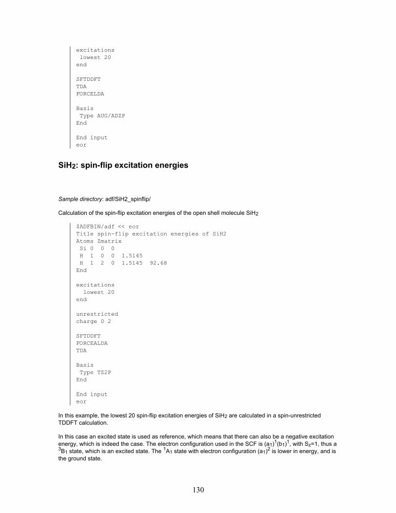
excitationslowest 20
end
SFTDDFTTDAFORCELDA
BasisType AUG/ADZP
End
End inputeor
SiH2: spin-flip excitation energies
Sample directory: adf/SiH2_spinflip/
Calculation of the spin-flip excitation energies of the open shell molecule SiH2
$ADFBIN/adf << eorTitle spin-flip excitation energies of SiH2Atoms ZmatrixSi 0 0 0H 1 0 0 1.5145H 1 2 0 1.5145 92.68
End
excitationslowest 20
end
unrestrictedcharge 0 2
SFTDDFTFORCEALDATDA
BasisType TZ2P
End
End inputeor
In this example, the lowest 20 spin-flip excitation energies of SiH2 are calculated in a spin-unrestrictedTDDFT calculation.
In this case an excited state is used as reference, which means that there can also be a negative excitationenergy, which is indeed the case. The electron configuration used in the SCF is (a1)1(b1)1, with Sz=1, thus a3B1 state, which is an excited state. The 1A1 state with electron configuration (a1)2 is lower in energy, and isthe ground state.
130

There is also an excited 1A1 state with electron configuration (b1)2. The transition from the ground 1A1 stateto the excited 1A1 state is an excitation from the electron configuration (a1)2 to (b1)2. This transition isactually a double excitation, which means that some double excitations can be reached using spin-flipTDDFT with carefully selected reference states.
In the MO → MO transitions part for the excitations of the output file, the spin of each molecular orbitals arealso specified to help assign the spin state of the excited states. Note that in these spin-flip calculations thetransitions are always from α spin-orbital to β or from β spin-orbital to α spin-orbital.
For open-shell molecules, spin-flip transition can result in transition to the ground state with a different Szvalue, while the symmetry of the transition density is A1. The excitation energy of this transition should bezero and this can be used to test the reliability of spin-flip TDDFT. Indeed the calculation of the spin-flipexcition energies of SiH2 shows one value which is close to zero and has a transition density of A1symmetry.
The 1A1 state with electron configuration (a1)2 can also be used in the calculation of the excitation energies.This is a closed shell configuration, in which case we do not need the spin-flip method.
$ADFBIN/adf << eorTitle excitation energies of SiH2Atoms ZmatrixSi 0 0 0H 1 0 0 1.5145H 1 2 0 1.5145 92.68
End
excitationslowest 20
end
BasisType TZ2P
End
End inputeor
The transition from the ground 1A1 state to the excited 1A1 state, which is an excitation from the electronconfiguration (a1)2 to (b1)2, can not be reached in this calculation, since it has mainly double excitationcharacter. Of course, other excited 1A1 states can be reached.
N2: TDHF excitation energies
Sample directory: adf/N2_TDHF/
Calculation of the excitation energies of N2 using time-dependent Hartree-Fock (TDHF). It also shows thepossibility to use the Tamm-Dancoff approximation (TDA). This examples consists of 4 calculations:
• non-relativistic TDHF• spin-orbit coupled TDHF• non-relativistic TDHF, TDA• spin-orbit coupled TDHF, TDA
The results will be inaccurate due to small basis set. The key ADDDIFFUSEFIT is required for a moreaccurate fit of the density.
131

$ADFBIN/adf << eorAtomsN 0 0 0N 0 0 1.0977End
XChartreefock
end
dependency bas=1e-4adddiffusefit
BasisType DZCore None
End
integration 10
excitationslowest 5
endEnd Inputeor
In case of spin-orbit coupling one needs to include the key RELATIVISTIC with argument ZORASPINORBIT. In practice one needs to calculate more excitations if one includes spin-orbit coupling, sincethe singlet-singlet and singlet-triplet excitations are not calculated separately, but will be treatedsimultaneously, since they may mix.
excitationslowest 20
endrelativistic spinorbit zora
The Tamm-Dancoff approximation (TDA) will be used if one includes the key TDA. The calculation is theneffectively a CIS calculation.
TDA
TiCl4: core excitation energies
Sample directory: adf/TiCl4_CoreExci/
Calculation of the 2p Ti and 2p Cl core excitation energies of TiCl4
$ADFBIN/adf << eorTitle TiCl4 TD-DFT scalar relativistic 2p Ti core excitations
UnitsLENGTH BOHR
End
132

AtomsTi 0. 0. 0.Cl 2.36754 2.36754 2.36754Cl -2.36754 -2.36754 2.36754Cl 2.36754 -2.36754 -2.36754Cl -2.36754 2.36754 -2.36754
EndSYMMETRY T(D)
EPRINTeigval 1000 1000
End
XCGGA LB94
End
relativistic scalar zora
ModifyExcitationUseOccupiedT2 2
SubEndUseScaledZORA
END
ExcitationONLYSINGDavidson &T2 12
SubEndEnd
BasisType DZCore None
End
end inputeor
In this example, the 12 lowest singlet-singlet excitation energies of T2 symmetry are calculated, the dipoleallowed excitations. This can also be achieved using the ALLOWED subkey in the key Excitation.
In this example only excitations from the 2t2-orbital are included (see the key MODIFYEXCITATION), analmost pure 2p core orbital of titanium. The orbital energies of the uninteresting other occupied orbitals areartificially changed to a large negative value (-1d6 hartree).
In the second example the 2p Cl core excitation energies of TiCl4 are calculated. The difference between thefirst example in this one is mainly the use of the key MODIFYEXCITATION:
ModifyExcitationUseOccRange -8.0 -6.0UseScaledZORA
END
In this example only excitations from occupied orbitals are considered which have orbital energies between-8 and -6 hartree, namely the 5a1, 1e, 1t1, 4t2, and 5t2 orbitals, which are almost pure 2p core orbitals of
133

chlorine. The orbital energies of the uninteresting other occupied orbitals are again artificially changed to alarge negative value (-1d6 hartree).
Ne: (core) excitation energies including spin-orbit coupling
Sample directories: adf/Ne_exciso/ and adf/Ne_CoreExci/
Calculation of the (core) excitation energies of Ne including spin-orbit coupling.
$ADFBIN/adf << eorTitle NeAtoms
Ne .0000 .0000 0.0000EndBasisType QZ4P
Endrelativistic scalar zorasymmetry d(8h)integration 6.0xcmodel SAOP
endExcitationslowest 10
End
ModifyExcitationUseOccupiedA1.g 1
SubEndUseScaledZORA
END
End inputeor
mv TAPE21 Frag.t21rm logfile TAPE21
$ADFBIN/adf << eorTitle Ne spin-orbitAtoms
Ne .0000 .0000 0.0000 f=FragEndrelativistic spinorbit zorasymmetry d(8h)xcmodel SAOP
endintegration 6.0Excitationslowest 12
End
134

ModifyExcitationUseOccupiedE1/2.g 1
SubEndUseScaledZORA
END
FragmentsFrag Frag.t21
EndSTCONTRIBEnd inputeor
The difference between the core excitation calculation and the standard excitation is the extra subkeyMODIFYEXCITATION in the core excitation calculation (in italic).
ADF can not handle ATOM and linear symmetries in excitation calculations. Therefore a subsymmetry isused, in this case symmetry d(8h).
A relatively large QZ4P basis set is used, which is still insufficient for excitations to Rydberg-like orbitals, oneneeds more diffuse functions.
The key STCONTRIB is used, which will give a composition of the spin-orbit coupled excitation in terms ofsinglet-singlet and singlet-triplet scalar relativistic excitations. In order to use the key STCONTRIB the scalarrelativistic fragment should be the complete molecule.
In this case the key MODIFYEXCITATION takes care that only excitations from the occupied 1s-orbital(spinor) are included. In symmetry d(8H) the 1s-orbital (spinor) is of A1.g (E1/2.g) symmetry.
AgI: excitation energies including spin-orbit coupling perturbatively
Sample directory: adf/AgI_asoexcit/
Calculation of the excitation energies of AgI including spin-orbit coupling in a perturbative way.
$ADFBIN/adf << eorTitle [AgI]AtomsAg .0000 .0000 2.5446I .0000 .0000 0.0000
Endrelativistic scalar zorasymmetry C(7v)integration 6.0Excitationslowest 60
EndSOPERTBasisType TZ2PCore None
135

Endeor
ADF can not handle ATOM and linear symmetries in excitation calculations. Therefore a subsymmetry isused, in this case symmetry C(7v).
A relatively small TZ2P basis set is used, which is not sufficient for excitations to Rydberg-like orbitals, oneneeds more diffuse functions.
The key SOPERT is included in scalar relativistic ZORA calculations of excitation energies. First scalarrelativistic TDDFT calculations are performed to determine the lowest 60 singlet-singlet and singlet-tripletexcited states and the spin-orbit coupling operator is applied to these single-group excited states to obtainthe excitation energies with spin-orbit coupling effects included.
N2: excited state geometry optimization
Sample directory: adf/EGO_N2/
Example for a singlet excited state geometry optimization, hybrid functional used.
Needed for such excited state optimizations are the key EXCITATIONS (to calculate excitation energies),the key GEOMETRY (to do a geometry optimization) and the key EXCITEDGO (to select for whichexcitation a geometryy optimization should be performed). In this case a hybrid functional B3LYP is used.
$ADFBIN/adf <<eorTITLE N2 Excited state geometryatoms
N 0.0 0.0 -0.7N 0.0 0.0 0.7
end
XCHYBRID B3LYP
END
Integration 5
GEOMETRYITERATIONS=30CONVERGE grad=0.0001
END
basisTYPE DZ
CORE NONEend
excitationsLOWEST 10onlysingletend
EXCITEDGOSTATE S-.u 1
136

OUTPUT=2end
ALLPOINTSeor
CH2: spin-flip excited state geometry optimization
Sample directory: adf/EGO_CH2_sf/
Example for a spin-flip excited state geometry optimization with a triplet reference, and a frequencycalculation afterwards.
Needed for such excited state optimizations are the key EXCITATIONS (to calculate excitation energies),the key GEOMETRY (to do a geometry optimization) and the key EXCITEDGO (to select for whichexcitation a geometryy optimization should be performed). In this case spin-flip excitations are calculated.
$ADFBIN/adf <<eorTITLE CH2 Excited state geometry with triplet reference and spin-flipexcitationatoms
C 0.000000 0.000000 0.0H 0.7 0.0 0.7H -0.7 0.0 0.7
endUNRESTRICTEDCHARGE 0 2GEOMETRYITERATIONS 50CONVERGENCE E=0.0001 grad=0.0001
ENDbasisTYPE DZP
CORE NONEendexcitationsLOWEST 10endTDASFTDDFTFORCEALDAEXCITEDGOSTATE B2 1OUTPUT=2
endSYMMETRY C(2V)eormv TAPE21 CH2.t21
Next the frequencies are calculated of the excited state. A restart is used to pick up the excited stategeometry of the previous calculation. Note that in a numerical FREQUENCIES calculation symmetry isturned off except to reduce the number of points calculated. Thus irrespective of the specified point groupsymmetry the symmetry label A of SYMMETRY NOSYM should be used to select the excited state. Care
137

should be taken to ensure that the correct state is chosen in this frequencies calculation as the excited statenumber can change when the point group is changed. In this case instead of 'B2 1' one needs to select 'A 2'.
$ADFBIN/adf <<eorTITLE CH2 Excited state frequencies with triplet reference and spin-flipexcitationatoms
C 0.000000 0.000000 0.0H 0.7 0.0 0.7H -0.7 0.0 0.7
endRESTART CH2.t21UNRESTRICTEDCHARGE 0 2GEOMETRYFREQUENCIES
ENDbasisTYPE DZP
CORE NONEendexcitationsLOWEST 10endTDASFTDDFTFORCEALDAEXCITEDGOSTATE A 2OUTPUT=2
endSYMMETRY C(2V)eor
Hyperpol: Hyperpolarizabilities of He and H2
Sample directory: adf/Hyperpol/
This sample illustrates the computation of (hyper) polarizability tensors for the He atom and the H2 molecule.
The symmetry is specified, because the Response module in ADF cannot yet handle the infinite symmetriesATOM, C(lin), D(lin).
$ADFBIN/adf <<EORTitle expt geometrie H2(VII),VWNnoprint sfo,frag,functions
Symmetry C(8v)
AtomsH 0 0 -0.37305H 0 0 0.37305
End
138

FragmentsH t21.H7
End
ResponseHyperPol 0.03DynaHypAllComponents
End
EField 0 0 0.001
end inputEOR
The Response data block specifies (AllComponents) that not only the (default) zz-dipole polarizability is tobe computed, but the complete tensor. The subkey HyperPol instructs the program to computehyperpolarizabilities and not only polarizabilities. The DynaHyp subkey implies that the frequency-dependent(hyper)polarizability is calculated. In that case the main laser frequency has to be specified, in hartree units,after the HyperPol subkey.
Only the first hyperpolarizability has been implemented in ADF. Some information on secondhyperpolarizabilities can be obtained from the calculation of the first one in a finite field (EFIELD).
In similar fashion the frequency-dependent hyperpolarizability is computed for He, but only the zzz-component because now the AllComponents subkey is omitted.
$ADFBIN/adf <<EORTitle hyperpolarizability He with the LB94 potentialnoprint sfo,frag,functions
AtomsHe 0 0 0
End
XCGGA LB94
END
FragmentsHe t21.He8
End
ResponseHyperPol 0.07DynaHyp
End
integration 5.0
EField 0 0 0.001
Symmetry C(8v)
end inputEOR
139

AgI: polarizabilities including spin-orbit coupling
Sample directory: adf/AgI_SO_Pol/
Example shows an frequency-dependent ZORA calculation of complex linear response of AgI including spin-orbit coupling.
The polarizability is calculated using the AORESPONSE key, in which spin-orbit coupling is taken intoaccount. In this case a spin-restricted calculation is required, but, unlike the rest of AORESPONSE, alsoNOSYM. In this example lifetime effects are included.
$ADFBIN/adf << eorTITLE AgI,SO-ZORAbasistype TZ2Pcore None
endATOMS
Ag 0.0 0.0 1.2723I 0.0 0.0 -1.2723
ENDsymmetry nosymintegration 6.0Relativistic zora spinorbitaoresponsescffrequency 1 0.085 HARTREElifetime 0.007ALDAEL_DIPOLE_EL_DIPOLE
endEND INPUTeor
HF: Dispersion Coefficients
Sample directory: adf/Disper_HF/
General dispersion coefficients (beyond de dipole-dipole C6 interaction coefficient) are computed with theauxiliary program DISPER. It uses two output files from previous ADF Response calculations. In theexample, the two ADF runs are one and the same and the relevant TENSOR output file is used twice.
$ADFBIN/adf <<EOR
title Van der Waals coefficients HF
atomsH 0 0 -0.8708056087F 0 0 0.04619439132end
140

BasisType DZPCore Small
End
symmetry C(8v)
RESPONSEMAXWAALS 8VANDERWAALS 7ALLTENSORALLCOMPONENTS
END
end inputEOR
Polarizabilities are computed at 7 (imaginary) frequencies between 0 and infinity. The program determinesinternally the actual frequency values in this range to use. The user only specifies the number of them,thereby determining the precision of, in fact, a numerical integration over the zero-infinity frequency range. Avalue of 7 is rather low.
MaxWaals determines that not only the C6 but also C7 and C8 coefficients are computed. A value higherthan 8 would not be recommended, because the available basis sets would be inadequate for highercoefficients.
In DISPER calculations the preparatory Response calculation must use the AllTensor and AllComponentssubkeys.
The calculation produces a file TENSOR. The subsequent DISPER run uses two such files. In this example,both are taken from the same ADF run, copying the TENSOR file to, respectively, tensorA and tensorB.These names are prescribed for a DISPER calculation.
cp TENSOR tensorAcp TENSOR tensorB
$ADFBIN/disper -n1 << eoreor
The DISPER program needs no other input than just the files tensorA and tensorB, which must both bepresent as local files. Note the '-n1' flag: this enforces that a single-node (non-parallel) run is performed. Thecurrent implementation does not support parallelization of DISPER, because the kid processes may nothave the (local to the master!) files tensorA and tensorB.
DMO: Circular Dichroism spectrum
Sample directory: adf/DMO_CD/
If the subkey CDSPECTRUM is included in the key EXCITATIONS, the rotatory strength is calculated for thecalculated excitations, in order to calculate the CD (Circular Dichroism) spectrum. Only useful for chiralmolecules.
With the VELOCITY keyword also the dipole-velocity representation of the rotatory strength is calculated.
141

Note: results will be physically meaningless due to small basis set. purpose of this job is to provide a testcase for the CD implementation
Do not use less strict convergence criteria than default, better to use tighter criteria. The approximations inthe evaluation of the integrals one makes with the linear scaling techniques are effectively switched off bysetting LINEARSCALING 100 (recommended to use this).
Usage:
$ADFBIN/adf <<eorTITLE dimethyloxirane excitations + CD
COMMENTresults will be physically meaningless due to small basis set.purpose of this job is to provide a test case for the CD implementation
END
XCgga becke perdew
END
BasisType DZPCore Small
End
ATOMSO 0.000129 1.141417 0.000023C -0.597040 -0.094320 0.428262C 0.596952 -0.094328 -0.428223H -0.442927 -0.302650 1.487698H 0.442944 -0.302474 -1.487720C -1.978779 -0.386617 -0.093924H -2.723275 0.220579 0.429114H -2.043506 -0.157697 -1.159810H -2.236045 -1.439970 0.055144C 1.978716 -0.386693 0.093893H 2.236030 -1.439985 -0.055498H 2.723156 0.220701 -0.429005H 2.043497 -0.158088 1.159845END
linearscaling 100excitationscdspectrumonlysingletvelocitylowest 10
end
END INPUTeor
Twisted Ethene: CD spectrum, hybrid functional
142

Sample directory: adf/Twist_Ethene_TDDFT/
If the subkey CDSPECTRUM is included in the key EXCITATIONS, the rotatory strength is calculated for thecalculated excitations, in order to calculate the CD (Circular Dichroism) spectrum. Only useful for chiralmolecules. A hybrid functional is used in this case.
With the VELOCITY keyword also the dipole-velocity representation of the rotatory strength is calculated.
Note: results will be physically meaningless due to small basis set. purpose of this job is to provide a testcase for the CD implementation
Do not use less strict convergence criteria than default, better to use tighter criteria. The approximations inthe evaluation of the integrals one makes with the linear scaling techniques are effectively switched off bysetting LINEARSCALING 100 (recommended to use this).
Usage:
$ADFBIN/adf <<eorTITLE twisted ethene
COMMENTpurpose of this job is to provide a test case for the CD implementationwith hybrid functionals, and to test the "velocity" keyword
END
XChybrid PBE0
END
BasisType TZ2PCore Small
End
ATOMSC 0.000000 0.000000 0.000000C -0.000000 -0.000000 1.350716H 0.565703 -0.745428 -0.540179H -0.565703 0.745428 -0.540179H 0.035837 -0.935093 1.890895H -0.035837 0.935093 1.890895END
linearscaling 99excitationscdspectrumonlysingletvelocitylowest 20
end
END INPUTeor
143
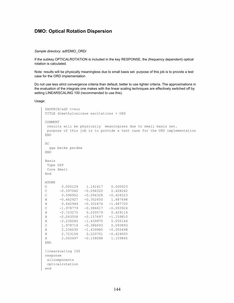
DMO: Optical Rotation Dispersion
Sample directory: adf/DMO_ORD/
If the subkey OPTICALROTATION is included in the key RESPONSE, the (frequency dependent) opticalrotation is calculated.
Note: results will be physically meaningless due to small basis set. purpose of this job is to provide a testcase for the ORD implementation
Do not use less strict convergence criteria than default, better to use tighter criteria. The approximations inthe evaluation of the integrals one makes with the linear scaling techniques are effectively switched off bysetting LINEARSCALING 100 (recommended to use this).
Usage:
$ADFBIN/adf <<eorTITLE dimethyloxirane excitations + ORD
COMMENTresults will be physically meaningless due to small basis set.purpose of this job is to provide a test case for the ORD implementation
END
XCgga becke perdew
END
BasisType DZPCore Small
End
ATOMSO 0.000129 1.141417 0.000023C -0.597040 -0.094320 0.428262C 0.596952 -0.094328 -0.428223H -0.442927 -0.302650 1.487698H 0.442944 -0.302474 -1.487720C -1.978779 -0.386617 -0.093924H -2.723275 0.220579 0.429114H -2.043506 -0.157697 -1.159810H -2.236045 -1.439970 0.055144C 1.978716 -0.386693 0.093893H 2.236030 -1.439985 -0.055498H 2.723156 0.220701 -0.429005H 2.043497 -0.158088 1.159845END
linearscaling 100responseallcomponentsopticalrotation
end
144

END INPUTeor
DMO: ORD, lifetime effects (key AORESPONSE)
Sample directory: adf/DMO_ORD_aoresponse/
If the subkey OPTICALROTATION is included in the key AORESPONSE, the (frequency dependent) opticalrotation is calculated. In this example lifetime effects are included. This test example consists of two ORDcalculations: one with and one without the velocity gauge.
Note: results will be physically meaningless due to small basis set. purpose of this job is to provide a testcase for the ORD implementation
Usage:
$ADFBIN/adf <<eorTITLE dimethyloxirane, ORDCOMMENTresults will be physically meaningless due to small basis set.purpose of this job is to provide a test case for the ORD implementation
ENDXC
gga becke perdewENDBasisType DZPCore Small
EndATOMSO 0.000129 1.141417 0.000023C -0.597040 -0.094320 0.428262C 0.596952 -0.094328 -0.428223H -0.442927 -0.302650 1.487698H 0.442944 -0.302474 -1.487720C -1.978779 -0.386617 -0.093924H -2.723275 0.220579 0.429114H -2.043506 -0.157697 -1.159810H -2.236045 -1.439970 0.055144C 1.978716 -0.386693 0.093893H 2.236030 -1.439985 -0.055498H 2.723156 0.220701 -0.429005H 2.043497 -0.158088 1.159845ENDallpointsaoresponseALDAopticalrotationfrequency 1 5893 angstromscf iter 20lifetime 0.007
endEND INPUTeor
145

In the second example the subkey OPTICALROTATION of the key AORESPONSE is changed intoVELOCIYORD:
aoresponseALDAVelocityORDfrequency 1 5893 angstromscf iter 20lifetime 0.007
end
Propene: damped Verdet constants
Sample directory: adf/DampedVerdet/
Specify the subkey MAGOPTROT in the AORESPONSE key to calculate the Verdet constant. Here it isspecified together with the LIFETIME key, such that the real and imaginary part of the damped Verdetconstant will be calculated.
$ADFBIN/adf <<eortitle Propene
ATOMSC 0.867000 1.441800 3.000000C 0.849400 2.777300 3.000000C 2.115500 0.591200 3.000000H -0.088300 0.909000 3.000000H -0.085900 3.336500 3.000000H 1.772400 3.363200 3.000000H 2.737100 0.793300 2.115200H 1.876900 -0.479100 3.000000H 2.737100 0.793300 3.884800END
basistype DZPcore None
end
SCFiterations 50converge 1.0e-6 1.0e-3mixing 0.2lshift 0.0diis n=10 ok=0.5 cyc=5 cx=5.0 cxx=10.0END
symmetry nosymallpoints
INTEGRATION 5.0linearscaling 9
XC
146

Model SAOPEND
noprint sfo
aoresponsescf converge 1d-5 iterations 25frequency 1 0.2 HartreeALDAgiaomagoptrotlifetime 0.007
end
end inputeor
H2O: Verdet constants
Sample directory: adf/H2O_Verdet/
Specify the subkey MAGOPTROT in the AORESPONSE key to calculate the Verdet constant.
$ADFBIN/adf <<eortitle water
basistype TZPcore None
end
atomsO 0.000000 0.134692 0.000000H 0.869763 -0.538741 0.000000H -0.869763 -0.538794 0.000000end
symmetry nosymallpoints
integration 6.0linearscaling 99
xclda vwngga revPBE
end
aoresponsescf converge 1d-6 iterations 25frequency 1 0.088558 HartreeALDAgiaomagoptrot
147

end
end inputeor
H2O: MCD
Sample directory: adf/H2O_MCD/
Example for the calculation of magnetic circular dichroism (MCD). If the subkey MCD is included in the keyEXCITATIONS the MCD parameters of the calculated excitations are calculated (A and B terms). The keysRELATIVISTIC ZORA and SOMCD are required for a calculation of temperature-dependent C terms. Thekey ALLPOINTS is required for an MCD calculation (if the molecule has symmetry).
$ADFBIN/adf <<eortitle water MCD
atomsO 0 0 0H 0 0 1H 0 1 0end
BASISTYPE DZPend
ALLPOINTS
SOMCD
UNRESTRICTED
CHARGE 1 1
RELATIVISTIC ZORA
excitationslowest 20onlysingletmcd NMCDTERM=5end
end inputeor
H2O: static magnetizability
Sample directory: adf/H2O_magnet/
Basic example for a magnetizability calculation.
148
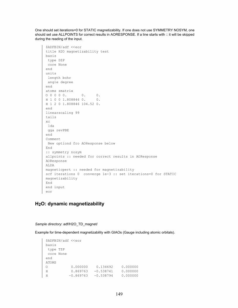
One should set iterations=0 for STATIC magnetizability. If one does not use SYMMETRY NOSYM, oneshould set use ALLPOINTS for correct results in AORESPONSE. If a line starts with :: it will be skippedduring the reading of the input.
$ADFBIN/adf <<eortitle H2O magnetizability testbasistype DZPcore None
endunitslength bohrangle degree
endatoms zmatrixO 0 0 0 0. 0. 0.H 1 0 0 1.808846 0. 0.H 1 2 0 1.808846 104.52 0.endlinearscaling 99tailsxcldagga revPBE
endCommentNew optiond fro AOResponse below
End:: symmetry nosymallpoints :: needed for correct results in AOResponseAOResponseALDAmagneticpert :: needed for magnetizabilityscf iterations 0 converge 1e-3 :: set iterations=0 for STATICmagnetizabilityEndend inputeor
H2O: dynamic magnetizability
Sample directory: adf/H2O_TD_magnet/
Example for time-dependent magnetizability with GIAOs (Gauge including atomic orbitals).
$ADFBIN/adf <<eorbasistype TZPcore None
endATOMSO 0.000000 0.134692 0.000000H 0.869763 -0.538741 0.000000H -0.869763 -0.538794 0.000000
149

ENDsymmetry nosymallpointsintegration 6.0linearscaling 99xclda vwngga revPBE
endaoresponsescf conv 1d-6 iter 25frequency 1 5893 AngstromgiaoALDAmagneticpertFitAOderiv
endEND INPUTeor
C2H4: Time-dependent current-density-functional theory
Sample directory: adf/C2H4_TDCDFT/
Calculation of excitation energies and response properties of C2H4, with the VK functional, thus using time-dependent current-density-functional theory.
$ADFBIN/adf << eortitle C2H4 excitation energy calculation with the VK functional
ATOMS1. C 0.000000 0.000000 0.6663182. C 0.000000 0.000000 -0.6663183. H 0.000000 0.928431 1.2393884. H 0.000000 -0.928431 1.2393885. H 0.000000 0.928431 -1.2393886. H 0.000000 -0.928431 -1.239388END
BASISC $ADFHOME/atomicdata/ET/ET-pVQZ/CH $ADFHOME/atomicdata/ET/ET-pVQZ/HEND
EXCITATIONSEND
CURRENTRESPONSEEND
endinputeor$ADFBIN/adf << eortitle C2H4 response calculation with the VK functional
150

ATOMS1. C 0.000000 0.000000 0.6663182. C 0.000000 0.000000 -0.6663183. H 0.000000 0.928431 1.2393884. H 0.000000 -0.928431 1.2393885. H 0.000000 0.928431 -1.2393886. H 0.000000 -0.928431 -1.239388END
BASISTYPE TZ2PEND
RESPONSEALLCOMPONENTSEND
CURRENTRESPONSEEND
endinputeor
NMR chemical shifts and spin-spin coupling constants
HBr: NMR Chemical Shifts
Sample directories: adf/HBr/ and adf/HBr_SO/
Computation of the NMR chemical shifts for HBr. The second sample uses spin-orbit relativistic corrections.
$ADFBIN/adf << eorTITLE HBr non-relativistic
ATOMS1. H .0000 .0000 .00002. Br .0000 .0000 1.4140
End
BasisType DZCore Large
End
XCGGA Becke Perdew
End
End inputeor
The TAPE21 result file of ADF must be present under that name for the NMR calculation
151

mv t21.nmr TAPE21
The NMR program uses only one input (block) key NMR, currently. The subkeys specify what output isproduced (OUT) and for which Nuclei the NMR data are computed and printed (NUC). See the User's Guideand the Utilities document for more details.
$ADFBIN/nmr << eorNMR
Out TENSNuc 1 2
Endeor
The second run is like the first, except that it uses relativistic corrections, including Spin-Orbit terms. Thisimplies that NOSYM symmetry must be used in the ADF calculation: the NMR program cannot handlesymmetry calculations in combination with spin-orbit terms and will stop with an error message if you try todo so.
$ADFBIN/adf << eorTITLE HBr relativistic spinorbit Pauli
Atoms1. H .0000 .0000 .00002. Br .0000 .0000 1.4140
End
BasisType DZCore Large
End
Symmetry NoSYM
XCGGA Becke Perdew
End
Relativistic SpinOrbit Pauli
End inputeor
rm t12.rel
$ADFBIN/nmr << eorNMR
OUT TENSNUC 1 2
Endeor
HgMeBr: NMR Chemical Shifts
152

Sample directories: adf/HgMeBr_pnr/ (non-relativistic), adf/HgMeBr_psc/ (Pauli scalar relativistic), adf/HgMeBr_zso/ (ZORA relativistic and Spin-Orbit terms included)
NMR data are computed for the 1st and 3rd nucleus only. The UIK subkey is used to indicate that certainterms are to be included in the 'U-matrix', which goes into the first-order change of the MO's due to theapplied magnetic field. See the documentation (Utilities) for more information.
The 'BEST' specification means that the mass-velocity and Darwin terms are included for a scalar relativisticcalculation. In a non-relativistic run it has no meaning. In a spin-orbit run it would include the Fermi-contactterm for the Pauli formalism, and the ZORA Spin-Orbit terms for a ZORA calculation.
$ADFBIN/nmr << eorNMR
U1K BESTNUC 1 3
ENDeor
The other two calculations are similar, apart from the specification of the applicable relativistic features.
CH4: NMR Chemical Shifts, SAOP potential
Sample directory: adf/CH4_SAOP/
Computation of the NMR chemical shifts for CH4, with the model potential SAOP.
Important: use SAVE TAPE10. This is necessary for SAOP, since the nmr program does not know aboutSAOP or other model potentials. On TAPE10 the SCF potential is written, which is read in by the nmrprogram.
Note: For SAOP one needs an all-electron basis set
$ADFBIN/adf << eorxcmodel saop
end
DefineRCH = 1.085XCH = sqrt(3)*(RCH/3)
End
AtomsC 0 0 0H XCH XCH XCHH XCH -XCH -XCHH -XCH XCH -XCHH -XCH -XCH XCH
End
BasisType TZ2PCore None
End
153

save TAPE10End Inputeor
$ADFBIN/nmr << eorNMR
Out TENSNuc 1 2
Endeor
CO: NMR Chemical Shifts, SIC-VWN potential
Sample directory: adf/CO_fc_SICVWN/
Computation of the NMR chemical shifts for CO, with the SIC-VWN potential.
Important: use SAVE TAPE10. This is necessary for SIC-VWN or SAOP, since the epr or nmr program doesnot know about SIC-VWN or other model potentials. On TAPE10 the SCF potential is written, which is readin by the epr or nmr program.
Note: adf with the SIC-VWN only runs serial correctly, and symmetry NOSYM is required.
Note: Both epr and nmr change TAPE10, TAPE21. Therefore use original TAPEs from adf.
$ADFBIN/adf -n1 << eorTITLE CO, SIC-VWN, Basis set TZ2PBasisType TZ2PCore Small
EndRELATIVISTIC Scalar PauliSYMMETRY NOSYMATOMS Z-mat
1 C 0 0 02 O 1 0 0 RCO
ENDGEOVAR
RCO 1.139719ENDINTEGRATION 6.0XC
LDA VWNENDSICOEP
IPRINT 1SELF 35
ENDSAVE TAPE10END INPUTeor
cp TAPE21 t21cp TAPE10 t10
154

$ADFBIN/epr -n1 << eorNMRSHIELDING
NUCLEI ALLOUTPUT
SIZE LARGESUBEND
ENDSICOEP
IPRINT 1ENDeor
rm TAPE10 TAPE15 TAPE21cp t21 TAPE21cp t10 TAPE10
$ADFBIN/nmr << eorNMR
U1K BESTENDeor
PF3: NMR Properties, Nucleus-independent chemical shifts
Sample directory: adf/Nmr_PF3/
Both the NMR program and the EPR/NMR program enables the calculation of so-called nucleus-independent chemical shifts. More details are available in the Properties Programs User's Guide.
In the ADF run, the Efield key is used to define points charges with zero charge. The GHOSTS key in thenmr or epr program then basically copies this block. For the interpretation of the results we refer to theliterature.
...Efield
3.0 4.0 5.0 0.01.0 2.0 3.0 0.0
End...eor
Example input for the EPR/NMR program.
$ADFBIN/epr -n1 << eorCLGEPR
NUCLEI ALLGHOSTS
3.0 4.0 5.01.0 2.0 3.0
SUBENDOUTPUT
SIZE LARGESUBEND
155

END
END INPUTeor
Example input for the NMR program.
$ADFBIN/nmr << eorNMR
Out Iso TensGHOSTS
3.0 4.0 5.01.0 2.0 3.0
SUBENDENDEND INPUTeor
PF3: Comparison of NMR with EPR/NMR
Sample directory: adf/PF3_nmr/
This example uses both the NMR program and the EPR/NMR program, which is somewhat different fromthe NMR program used in the examples above. Please check the Property Programs User's Guide for adiscussion on the advantages and disadvantages of the two implementations. This example explicitlycompares the two.
$ADFBIN/nmr << eorNMR
U1K BESTENDeor
The NMR program can currently formally be run in parallel. Due to certain single-CPU bottlenecks, this ishardly noticeable at the moment though. For this reason, there is currently limited advantage in using morethan one CPU for the nmr program. Most other property programs can currently not be run in parallel at alland require the -n1 flag.
The output of the two NMR calculations should be virtually identical.
$ADFBIN/epr -n1 << eorCLGEPR
NUCLEI ALLOUTPUT
SIZE LARGESUBEND
END
END INPUTeor
156

PF3: NMR with B3LYP
Sample directory: adf/NMR_B3LYP/
This example shows how to do hybrid calculation of NMR chemical shifts.
One needs of course a hybrid functional in the XC block key in ADF. One should also SAVE TAPE10, suchthat it is an input file in the nmr module.
$ADFBIN/adf << eortitle PF3-NMR-B3LYPbasistype DZPcore None
endDefine
RPF = 1.641314AXPF = 119.702107
EndAtomsP 0.00000000 0.00000000 1.00000000F -0.71283358 1.23466398 1.81325568F -0.71283358 -1.23466398 1.81325568F 1.42566716 0.00000000 1.81325568Endintegration 6.0noprint sfoxchybrid B3LYP
endsave TAPE10end inputeorrm logfile
$ADFBIN/nmr << eorNMR
Out TENSNuc 1 2SCF 1.d-4
Endeor
Next the same calculation is performed with the scalar relativistic ZORA Hamiltonian. In that case oneshould include in the ADF calculation.
RELATIVISTIC SCALAR ZORA
In the last example spin-orbit coupling is included. Symmetry should be NOSYM.
symmetry nosymRELATIVISTIC SPINORBIT ZORA
In the input for the nmr module one can add the key ZSOAO2007 to approximate the effect of spin on thenucleus in the spin-orbit coupled calculations.
157

VOCl3: NMR Chemical shifts
Sample directory: adf/Nmr_VOCl3/
After a scalar relativistic Pauli calculation in ADF, using NOSYM, the EPR/NMR program is invoked.TheEPR/NMR program does not support ZORA at the moment.
$ADFBIN/adf << eorTITLE VOCl3
CHARGE 0
ATOMS Z-mat1 V 0 0 02 O 1 0 0 RVO3 Cl 1 2 0 RVCl AOVCl4 Cl 1 2 3 RVCl AOVCl 120.5 Cl 1 2 3 RVCl AOVCl -120.
END
INTEGRATION 5.0 5.0
GEOVARRVO 1.584452RVCl 2.164767AOVCl 108.614124
END
SYMMETRY NOSYM
RELATIVISTIC Scalar Pauli
XCLDA VWN
END
FRAGMENTSV t21.VO t21.OCl t21.Cl
END
COREPOTENTIALS t12.rel &V 1Cl 2O 3
END
END INPUTeor
The NUCLEI key now specifies that all atoms are to be treated for NMR. Much output is demanded.
$ADFBIN/epr -n1 << eorCLGEPR
158

NUCLEI ALLOUTPUT
SIZE LARGESUBEND
ENDEND INPUTeor
C2H2: NMR Spin-spin coupling constants
Sample directory adf/CPL_C2H2
Nonrelativistic calculation
A calculation of NMR nuclear spin-spin coupling constants (NSCCs).
As explained in the 'ADF Properties Programs' documentation, the quality of a calculation for spin-spincoupling constants, using the program 'CPL', depends largely on the preceding ADF calculation, whichproduces the Kohn-Sham orbitals and orbital energies, used as a starting point.
One of the quality-determining factors is the chosen basis set. It should be sufficiently flexible near thenucleus. Although the all-electron basis TZ2P is chosen in this example, it is recommendable to add morefunctions to the basis and fit sets near the nucleus in case of heavy elements. One could start from a ZORA/QZ basis for example.
The integration accuracy in the ADF calculation is chosen such that the region near the nuclei is describedrelatively more accurately than the rest of the molecule.
INTEGRATIONaccint 5accsph 6end
The NOSYM symmetry currently needs to be specified in ADF to enable the CPL program to work correctly.
The first call to cpl is as follows:
$ADFBIN/cpl <<eornmrcouplingdsopsosdscf convergence 1e-7nuclei 1 2 3 4nuclei 3 4endendinputeor
The CPL program can run in parallel.
The specification of what needs to be calculated is given in the nmrcoupling block key.
159

In this first example, the SD subkey is left out, as this would lead to a very strong increase in the requiredCPU time. The SD subkey is included in the second CPL run. That subkey controls the calculation of the so-called spin-dipole term.
The subkeys dso and pso specify that, respectively, the diamagnetic and paramagnetic orbital terms will becalculated. The often dominant Fermi contact term (FC) is calculated by default and therefore does not haveto be specified explicitly.
The scf convergence subkey, in this context, refers to the convergence for the solution of the coupled-perturbed Kohn-sham equations which need to be solved to obtain to spin-spin couplings.
The lines
nuclei 1 2 3 4nuclei 3 4
that one coupled-perturbed Kohn-Sham calculation is performed where nucleus number 1 (according to theordering in the ADF output) is the perturbing nucleus, and nuclei 2, 3, and 4 are the perturbed nuclei, andanother coupled-perturbed Kohn-Sham calculation is performed where nucleus 3 is the perturbing nucleusand nucleus 4 is the perturbed nucleus.
The second CPL run also includes the spin-dipole (SD) term, through the SD subkey.
The output of the CPL program first contains a lot of general information, a summary of the specified input,and then produces the desired numbers:
It prints separately the different contributions (FC, DSO, PSO, SD) if specified in input and sums them up toa total number. Experimental NSCCs between two nuclei A and B are usually reported as J(A,B) in Hertz.From a computational point of view, the so-called reduced NSCCs K(A,B) are more convenient forcomparisons. CPL outputs both. In this example, the Fermi-contact term is indeed dominant.
The first part of the output refers to the line
nuclei 1 2 3 4
then the same thing is done for the second similar line where nucleus 3 is the perturbing nucleus.
The output for the second CPL run looks very similar, but now the SD term is added to the Fermi contactterm, resulting in much longer execution times.
Scalar relativistic and spin-orbit calculations
The CPL program also enables calculations using scalar relativistic effects (ZORA) and/or spin-orbit effects.
Schematically, this requires the following changes to the input file with respect to a regular spin-orbitcalculation and a nonrelativistic CPL calculation:
• steep (1s) functions may need to be added to the standard basis sets.• the full-potential option for ZORA is needed in the create runs and all further runs:
relativistic zora scalar full• the molecular ADF calculation should contain the line
relativistic zora full spinorbit• the CPL input is unmodified with respect to the example given here. Please check the 'ADF
Property Programs' document for details on relativistic input options.
160

HF: NMR Spin-spin coupling constants, hybrid PBE0
Sample directory adf/CPL_HF_hybrid
A calculation of NMR nuclear spin-spin coupling constants (NSCCs) for the hybrid PBE0.
The hybrid PBE0 is chosen as exchange-correlation potential in the ADF calculation. The key 'usespcode' isrequired for consistency reasons of the PBE0 implementation in ADF and the kernel that is used in the 'CPL'program, that calculates NMR spin-spin coupling constants. Symmetry should be NOSYM. The basis setsused are specially optimized all-electron basis sets for NMR spin-spin coupling calculations (in the directory$ADFHOME/atomicdata/ZORA/jcpl), which have extra tight functions, compared to a default ADF basis set.The integration accuracy is extra high in the core region.
$ADFBIN/adf <<eorUNITS
length Angstromangle Degree
END:: experimental bond lengthATOMSF 0.0000 0.0000 0.0000H 0.0000 0.0000 0.9170ENDBASISType ZORA/jcplCore NoneENDusespcodeXChybrid PBE0
ENDSYMMETRY nosymSCFconverge 1.0e-8 1.0e-6ENDINTEGRATIONaccint 6.0accsph 7.5
endscfconverge 1e-8 1e-7
endend inputeor
The first call to cpl is as follows:
$ADFBIN/cpl <<eorgganmrcouplingdsopsoscf convergence 1e-6 iterations 20nuclei 1 2
end
161

endinputeor
The key 'gga' is included to use the first-order GGA potential instead of the first-order VWN potential. TheHartree-Fock part of the kernel is included automatically if a hybrid potential is used in the ADF calculation.
The second CPL run also includes the spin-dipole (SD) term, through the SD subkey, which is much moretime-consuming.
sd
PbH4: NMR Spin-spin coupling constants, finite nucleus
Sample directory: adf/PbH4_finitenuc/
Example for a finite nucleus calculation and the calculation of NMR spin-spin coupling constants.
One of the quality-determining factors for the calculation of NMR coupling constants is the chosen basis set,especially one needs enough tight s functions. If one has a large enough basis set in the core region onecan see an effect of using a finite size of the nucleus instead of a point nucleus, especially for heavy nuclei.Such large basis sets can be found for some elements in $ADFRESOURCES/ZORA/jcpl, which are basissets especially designed for NMR spin-spin coupling calculations. In this example first a basis set for Pb ismade which has many tight s functions.
cat < eor > $PWD/PbPb Basis TZ2P - all steep, plus high exponent fcts.
BASIS1s 39358.23035822071s 20080.72977460241s 10245.27029316451s 5227.178721002291s 2666.927918878721s 1360.677509632001s 694.2232192000001s 354.1955200000001s 180.7120000000002p 39358.23035822072p 20080.72977460242p 10245.27029316452p 5227.178721002292p 2666.927918878722p 1360.677509632002p 694.2232192000002p 354.1955200000002p 180.712000000000
1S 92.2002S 106.0002S 40.2003S 51.1503S 21.8504S 13.4004S 9.5505S 7.650
162
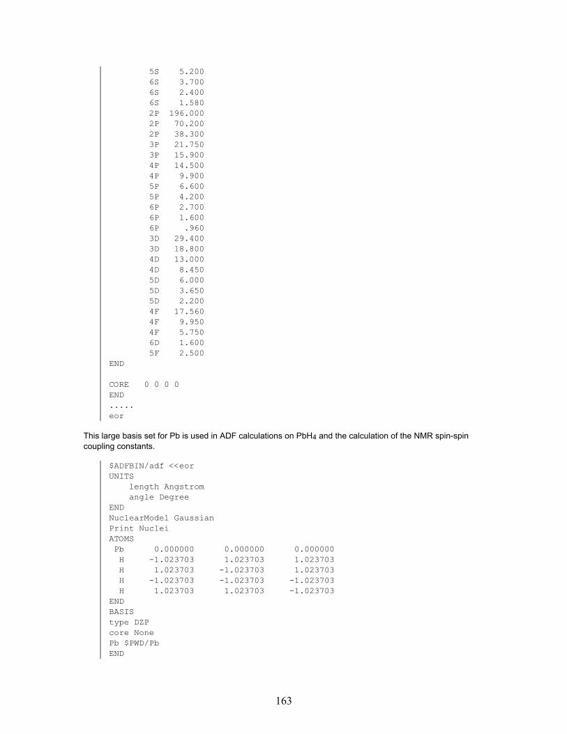
5S 5.2006S 3.7006S 2.4006S 1.5802P 196.0002P 70.2002P 38.3003P 21.7503P 15.9004P 14.5004P 9.9005P 6.6005P 4.2006P 2.7006P 1.6006P .9603D 29.4003D 18.8004D 13.0004D 8.4505D 6.0005D 3.6505D 2.2004F 17.5604F 9.9504F 5.7506D 1.6005F 2.500
END
CORE 0 0 0 0END.....eor
This large basis set for Pb is used in ADF calculations on PbH4 and the calculation of the NMR spin-spincoupling constants.
$ADFBIN/adf <<eorUNITS
length Angstromangle Degree
ENDNuclearModel GaussianPrint NucleiATOMSPb 0.000000 0.000000 0.000000H -1.023703 1.023703 1.023703H 1.023703 -1.023703 1.023703H -1.023703 -1.023703 -1.023703H 1.023703 1.023703 -1.023703
ENDBASIStype DZPcore NonePb $PWD/PbEND
163

XCgga PBE
ENDusespcodeSCFiterations 100converge 1.0e-8 1.0e-6ENDINTEGRATIONaccint 5.0accsph 10.0
endrelativistic scalar zoraend inputeor
$ADFBIN/cpl <<eorggaPrint Nucleinmrcouplingscf convergence 1e-5 iterations 25nuclei 1 2
endendinputeor
ESR / EPR properties
TiF3: ESR g-tensor, A-tensor, Q-tensor
Sample directory: adf/ESR_TiF3/
You calculate Electron Spin Resonance properties with the keywords ESR and QTENS. ESR is a block-typekey and is used to compute the G-tensor or the Nuclear Magnetic Dipole Hyperfine interaction. QTENS is asimple key and invokes the computation of the Nuclear Electric Quadrupole Hyperfine interaction.
Proper usage of the key ESR requires that you do one of the following:
(a) A Spin-Orbit calculation, spin-restricted, with exactly one unpaired electron, or(b) A Spin-Orbit calculation, spin-unrestricted in the collinear approximation, or(c) No Spin-Orbit terms and spin-unrestricted.
In case (a) and (b) you obtain the G-tensor. In case (b) and (c) you get the Magnetic Dipole Hyperfineinteraction.
Note: in case (a) the program also prints a Magnetic Dipole Hyperfine interaction data, but these have thenbeen computed without the terms from the spin-density at the nucleus.Note: in case (b) and (c) one can have more than one unpaired electron.Note: in case (b) one has to use symmetry NOSYM.
Five calculations are performed:
• Scalar relativistic spin-unrestricted
164

• Spin-Orbit relativistic spin-restricted• Scalar relativistic spin-restricted• Scalar relativistic open shell spin-restricted• Spin-Orbit relativistic spin-unrestricted collinear
After the preliminary calculations (DIRAC, to get the relativistic TAPE12 file with relativistic potentials, andthe Create runs), we first calculate the Dipole Hyperfine interaction: a spin-unrestricted calculation withoutSpin-Orbit coupling.
$ADFBIN/adf << eortitle TiF3 relativistic open shell unrestrictednoprint sfo,frag,functions
DEFINERTIF = 1.780RY = RTIF*SQRT(3)/2
END
esrend
qtens
atomsTi 0 0 0F RTIF 0 0F -RTIF/2 RY 0F -RTIF/2 -RY 0
end
fragmentsTi t21.tiF t21.f
end
xcGGA Becke Perdew
end
charge 0 1unrestricted
relativistic scalar zoraCorepotentials t12.rel &
Ti 1F 2
end
end inputeor
Then, for the same molecule, we compute the G-tensor in a Spin-Orbit run (spin-restricted).
The here-computed and printed Dipole Hyperfine interaction misses the terms from the spin-density at thenucleus: compare with the outcomes from the first calculation.
In each of the calculations, the QTENS key invokes the computation of the Electric Quadrupole Hyperfineinteraction.
165

Note that an all-electron calculation is carried out. This is relevant for the computation of the A-tensor, thenuclear magnetic dipole hyperfine interaction, where an accurate value of the spin-polarization density at thenucleus is important. For the G-tensor (and also for the Q-tensor) this plays a minor role, but for reasons ofconsistency both calculations use the same basis set and (absence of) frozen core.
$ADFBIN/adf << eortitle TiF3 relativistic spinorbit open shell restrictednoprint sfo,frag,functions
DEFINERTIF = 1.780RY = RTIF*SQRT(3)/2
END
esrend
qtens
atomsTi 0 0 0F RTIF 0 0F -RTIF/2 RY 0F -RTIF/2 -RY 0
end
fragmentsTi t21.tiF t21.f
end
xcGGA Becke Perdew
end
relativistic spinorbit zoraCorepotentials t12.rel &
Ti 1F 2
end
end inputeor
Next a scalar relativistic spin-restricted calculation is performed. The TAPE21 of this calculation is saved asa fragment in the next spin-unrestricted calculation, using only 1 SCF iteration, which is a way to get thescalar relativistic spin-restricted open shell result for the magnetic dipole hyperfine interaction.
$ADFBIN/adf << eortitle TiF3 scalar relativistic restrictednoprint sfo,frag,functions
DEFINERTIF = 1.780RY = RTIF*SQRT(3)/2
END
166

atomsTi 0 0 0F RTIF 0 0F -RTIF/2 RY 0F -RTIF/2 -RY 0
end
fragmentsTi t21.tiF t21.f
end
xcGGA Becke Perdew
end
relativistic scalar zoraCorepotentials t12.rel &
Ti 1F 2
end
end inputeor
mv TAPE21 t21.TiF3rm logfile
$ADFBIN/adf << eortitle TiF3 scalar relativistic open shell restrictednoprint sfo,frag,functions
DEFINERTIF = 1.780RY = RTIF*SQRT(3)/2
END
esrend
qtens
atomsTi 0 0 0 f=TiF3F RTIF 0 0 f=TiF3F -RTIF/2 RY 0 f=TiF3F -RTIF/2 -RY 0 f=TiF3
end
fragmentsTiF3 t21.TiF3
end
xcGGA Becke Perdew
end
167

charge 0 1unrestricted
scfiter 0
end
relativistic scalar zoraCorepotentials t12.rel &
Ti 1F 2
end
end inputeor
Finally a spin-orbit coupled spin-unrestricted calculation is performed using the collinear approximation. Notethat symmetry NOSYM is used.
$ADFBIN/adf << eortitle TiF3 relativistic spinorbit open shell unrestricted collinearnoprint sfo,frag,functions
DEFINERTIF = 1.780RY = RTIF*SQRT(3)/2
END
esrend
qtens
symmetry nosymunrestrictedcollinear
atomsTi 0 0 0F RTIF 0 0F -RTIF/2 RY 0F -RTIF/2 -RY 0
end
fragmentsTi t21.tiF t21.f
end
xcGGA Becke Perdew
end
relativistic spinorbit zoraCorepotentials t12.rel &
Ti 1F 2
168

end
end inputeor
VO: collinear approximation, ESR g-tensor, A-tensor, Q-tensor
Sample directory: adf/VO_collinear/
The ESR parameters of VO are calculated with the collinear approximation for unrestricted Spin-Orbitcoupled calculations. In this example the VO-molecule has three unpaired electrons.
You calculate Electron Spin Resonance properties with the keywords ESR and QTENS. ESR is a block-typekey and is used to compute the G-tensor or the Nuclear Magnetic Dipole Hyperfine interaction. QTENS is asimple key and invokes the computation of the Nuclear Electric Quadrupole Hyperfine interaction.
Proper usage of the key ESR requires that you do one of the following:
(a) A Spin-Orbit calculation, spin-restricted, with exactly one unpaired electron, or(b) A Spin-Orbit calculation, spin-unrestricted in the collinear approximation, or(c) No Spin-Orbit terms and spin-unrestricted.
In case (a) and (b) you obtain the G-tensor. In case (b) and (c) you get the Magnetic Dipole Hyperfineinteraction.
Note: in case (a) the program also prints a Magnetic Dipole Hyperfine interaction data, but these have thenbeen computed without the terms from the spin-density at the nucleus.Note: in case (b) and (c) one can have more than one unpaired electron.Note: in case (b) one has to use symmetry NOSYM.
Two calculations are performed:
• Scalar relativistic spin-unrestricted• Spin-Orbit relativistic spin-unrestricted collinear
After the preliminary calculations (DIRAC, to get the relativistic TAPE12 file with relativistic potentials, andthe Create runs), we first calculate the Dipole Hyperfine interaction: a spin-unrestricted calculation withoutSpin-Orbit coupling.
Note that one has to use ALLPOINTS in the calculation for a linear molecule to get results for the nuclearmagnetic dipole hyperfine interaction.
$ADFBIN/adf << eorAtomsV 0 0 0O 0 0 1.589
End
XCGGA Becke Perdew
End
esrendqtens
169

allpointsunrestrictedcharge 0 3
Relativistic Scalar ZORACorePotentials t12.rel &V 1O 2
End
integration 5
FragmentsV t21.VO t21.O
EndEnd inputeor
Then a spin-orbit coupled spin-unrestricted calculation is performed using the collinear approximation. Notethat symmetry NOSYM is used.
$ADFBIN/adf << eorAtomsV 0 0 0O 0 0 1.589
End
XCGGA Becke Perdew
End
esrendqtens
symmetry nosymunrestrictedcollinear
Relativistic Spinorbit ZORACorePotentials t12.rel &V 1O 2
End
integration 5
FragmentsV t21.VO t21.O
EndEnd inputeor
170

Ge+ and H2+: ESR g-tensor (epr program)
Sample directories: adf/Epr_Ge2+ and adf/Epr_H2+
The NMR/EPR program gives functionality that partially overlaps and partially differs from the ESR keywordinside ADF. Please check the ADF and Property Programs User's Guides for details.
In this example a scalar relativistic Pauli calculation is performed (ZORA is not implemented in thisprogram).
The preparatory ADF calculation can run parallel, the EPR module should run serial. The ADF calculationshould not use symmetry. It uses a high numerical integration accuracy. The revised PBE functional isinvoked. The implementation allows spin-unrestricted high-spin inputs and as does the ESR implementationwithin ADF itself.
The H2+ example is very similar and in fact a but simpler, so it will not be discussed separately here.
$ADFBIN/adf << eor
TITLE Ge2+, scf
SYMMETRY NOSYM
UNRESTRICTED
CHARGE +1 3
ATOMS Cart1 Ge 0.0000 0.0000 -1.23442 Ge 0.0000 0.0000 1.2344
END
INTEGRATION 6.0
FRAGMENTSGe t21.Ge
END
COREPOTENTIALS t12.rel &Ge 1
END
XCGGA revPBE
END
RELATIVISTIC Scalar Pauli
END INPUTeor
The EPR calculation itself then has a fairly simple input. It uses the TAPE21 file generated by ADF. The fullEPR G-tensor is printed, including an extensive analysis for the contribution of different terms.
The input line
171

NUCLEI NONE
implies that no NMR calculation is requested.
$ADFBIN/epr -n1 << eorCLGEPR
EPRGTSUBENDNUCLEI NONEOUTPUT
EPRSIZE LARGESUBEND
ENDEND INPUTeor
NF2: spin-other-orbit contribution g-tensor
Sample directory: adf/EPR_SOO
In this example the spin-other-orbit contribution to the g-tensor G(SOO) is calculated with the EPR module.
The NMR/EPR program gives functionality that partially overlaps and partially differs from the ESR keywordinside ADF. Please check the ADF and Property Programs User's Guides for details. The spin-other-orbitcontribution to the g-tensor is not something that can be calculated with the ESR option inside ADF.
The preparatory ADF calculation can run parallel, the EPR module should run serial. The ADF calculationshould use symmetry NOSYM, and an all electron basis set is required for the calculation of the G(SOO)term. TAPE10 is saved, which is necessary if special XC-potentials are used, like SIC or SAOP.
$ADFBIN/adf << eorUnrestrictedCharge 0 1Atoms
N 0.000000 0.000000 0.611280F 0.000000 -1.090100 -0.237720F 0.000000 1.090100 -0.237720
ENDXC
GGA Becke PerdewENDBasisType DZCore None
EndSymmetry NOSYMSAVE TAPE10, TAPE15eor
The EPR calculation itself then has a fairly simple input. It uses the TAPE21, TAPE10, and TAPE15 filesgenerated by ADF. The full EPR G-tensor is printed, including an extensive analysis for the contribution ofdifferent terms, including the (small) spin-other-orbit contribution to the g-tensor G(SOO).
172

The spin-other-orbit contribution to the g-tensor G(SOO) is calculated by including the subsubkey SOO inthe subkey EPRGT of the key CLGEPR. Note that the calculation can take very long, if one uses a largerbasis set, and a better integration grid. Both are in fact necessary for reliable results.
$ADFBIN/epr -n1 << eorCLGEPR
EPRGTSOO
SUBENDNUCLEI NONEOUTPUT
EPRSIZE LARGESUBEND
ENDEND INPUTeor
EFG, Mössbauer
Ferrocene: Mössbauer spectroscopy
Sample directory: adf/Mossbauer/
By default in ADF the electron density at the nuclei is calculated, no input key is required. The electrondensity at the nuclei could be used for the interpretation of isomer shifts in Mössbauer spectroscopy. Theabsolute electron density at a nucleus heavily depends on the accuracy of the basis set in the core region ofthis nucleus, especially if relativistic effects are included. Important is to use the same basis set, sameexchange correlation functional, same integration accuracy, if electron densities at nuclei in differentmolecules are compared. For the calculation of Mössbauer quadrupole splittings the key QTENS is required.For 57Fe quadrupole splittings will be written in units of mm/s, used in Mössbauer spectroscopy Exampleshows a calculation on ferrocene with a non-relativistic, and two with a scalar relativistic ZORA Hamiltonianusing a different all electron basis set.
First a non-relativistic calculation.
$ADFBIN/adf << eortitle ferrocene
AtomsFE 0.000000 0.000000 0.000000C 1.215650 0.000000 1.600813C 0.375656 -1.156152 1.600813C -0.983481 -0.714541 1.600813C -0.983481 0.714541 1.600813C 0.375656 1.156152 1.600813C 1.215650 0.000000 -1.600813C 0.375656 1.156152 -1.600813C -0.983481 0.714541 -1.600813C -0.983481 -0.714541 -1.600813C 0.375656 -1.156152 -1.600813H 2.310827 0.000000 1.629796H 0.714085 -2.197727 1.629796H -1.869498 -1.358270 1.629796
173

H -1.869498 1.358270 1.629796H 0.714085 2.197727 1.629796H 2.310827 0.000000 -1.629796H 0.714085 2.197727 -1.629796H -1.869498 1.358270 -1.629796H -1.869498 -1.358270 -1.629796H 0.714085 -2.197727 -1.629796
End
xcgga blyp
end
BasisType TZPCore none
End
qtens
Integration 6exactdensity
End Inputeor
Next the scalar relativistic ZORA calculations. ADF will also calculate the quadrupole splittings including thesmall component density, also called SR ZORA-4. The only difference is the RELATIVISTIC keyword:
relativistic scalar zora
Next a scalar relativistic calculation is performed with a much larger basis set (QZ4P) in the core region.Changing the basis set will have a large effect on the electron density at the nucleus and a noticeable effecton the calculated quadrupole splittings.
BasisType QZ4PCore none
Endrelativistic scalar zora
174

Analysis
Fragment orbitals and bond energy decomposition
Ni(CO)4: Compound Fragments
Sample directory: adf/Frags_NiCO4/
An illustration of the fragment feature of adf
A transition metal complex is built from a Nickel atom and four CO fragments. The outcomes allows for ananalysis (of molecular orbitals and the Bonding energy) in terms of the fragment properties. It is a SinglePoint calculation. Geometry optimization would not have been possible in this set-up because anoptimization requires that only single-atom fragments are used.
The three atoms are created first: C, O, and Ni. For Carbon and Oxygen a type-DZ basis set is used(double-zeta) using the Basis key, while Ni gets a type-TZP basis (triple-zeta plus polarization).
CO
The CO molecule, to serve as a fragment template in Ni(CO)4, is computed from the atomic fragments Cand O. The coordinate values (atoms) are in bohr, rather than in Angstrom because the unit-of-length isredefined by the key units with subkey length.
The key scf is used to specify a somewhat tighter convergence criterion than the default, just to illustratehow to do this (normal settings are quite adequate).
The TAPE21 result file is renamed t21.CO.
$ADFBIN/adf <<eortitle CO (as fragment for NiCO4)
SCFconverge 1e-8end
EPRINTSFO eig ovlEND
unitslength bohrend
atomsC 0 0 0O 0 0 2.15617844end
BasisType DZ
175

Core SmallEnd
endinputeor
mv TAPE21 t21.CO
Starting from ADF2008.01 one needs to include the subkey SFO of the key EPRINT with arguments eig andovl in order to get the SFO MO coefficients and SFO overlap matrix printed on standard output.
Main calculation
Apart from the title, the input contains comment. This does not specify computational parameters but is onlyechoed in the output header, similar to the title. Contrary to the title, however, such comments are notpreserved, apart from their echo in output and they are not written to TAPE21 or any other result file.
The atomic coordinates (atoms) are given in bohr (Units). To supply the numerical values use is made ofuser-defined constants (define): xyzC and xyzOx. This is convenient and it prevents typing errors whenseveral coordinate values are identical, in particular when they carry a lot of decimal places.
The Atoms records contain also a specification of the fragments to which the respective atoms belong: fourdifferent CO fragments. No fragment is specified for the Ni atom, which implies that it is a fragment on itsown.
The numbers at the very left of the records (1 through 9, with (optionally) a period after them), have norelevance. You can set them for ease of reference or counting.
$ADFBIN/adf <<eortitle Ni(CO)4, from fragments Ni and CO
COMMENTNo geometry optimization possible, because not all fragmentsare single atomsEND
unitslength bohr
end
EPRINTSFO eig ovlEND
DEFINExyzC=2.0053211xyzOx=3.2501913END
atoms1. Ni 0 0 02. C xyzC xyzC xyzC f=CO/13. C -xyzC -xyzC xyzC f=CO/24. C xyzC -xyzC -xyzC f=CO/35. C -xyzC xyzC -xyzC f=CO/46. O xyzOx xyzOx xyzOx f=CO/1
176

7. O -xyzOx -xyzOx xyzOx f=CO/28. O xyzOx -xyzOx -xyzOx f=CO/39. O -xyzOx xyzOx -xyzOx f=CO/4end
fragmentsCO t21.CONi t21.Niend
endinputeor
PtCl4H22-: Fragments again
Sample directory: adf/Frags_PtCl4H2
The (scalar) relativistic option (Pauli formalism) is used because of the presence of the relativistic Pt atom.The complex is built from fragments H2 and PtCl42-.
Dirac: relativistic core potentials
The program dirac is applied to generate the corepotentials file for all involved atom types, includingHydrogen. The latter has no frozen core, let alone a relativistic one, but the corepotentials file also containsthe total (relativistic) atomic potential. The (relativistic) atomic total potential is used in some types ofrelativistic options only, but it is a good idea to simply always run DIRAC for all the atoms whenever you doa relativistic calculation.
$ADFBIN/dirac <$adfresources/Dirac/Cl.2p$ADFBIN/dirac <$adfresources/Dirac/Pt.4d$ADFBIN/dirac <$adfresources/Dirac/H
mv TAPE12 t12.rel
The script above generates one TAPE12 file. The second and third dirac runs recognize the presence of theTAPE12 file (with the standard name 'TAPE12') that resulted from the earlier ones and they write theirresulting data to the tail of it.
Basic atoms, non-default settings
$ADFBIN/adf <<eorCreate H file=$ADFRESOURCES/DZP/HXC
LDA vwnGGA becke perdew
End
Relativistic ScalarCorePotentials t12.rel &
H 3EndEnd Input
177

eor
mv TAPE21 t21H
The final calculations of the molecule and larger fragments are performed with gga ('NonLocal') xccorrections. Although it is not necessary to use the same settings in the Create runs, applying them looks'nicer' and gives a better approximation of the bond energy of the molecule with respect to the basic atoms.Here it serves to show that also in a Create run various options can be used.
$ADFBIN/adf <<eorcreate Cl file=$ADFRESOURCES/DZP/Cl.2pxc
lda vwnGGA becke perdew
end
relativistic scalarcorepotentials t12.rel &
Cl 1end
end inputeor
mv TAPE21 t21Cl
$ADFBIN/adf <<eorCreate Pt file=$ADFRESOURCES/DZ/Pt.4dXC
lda vwnGGA becke perdew
End
Relativistic scalarCorePotentials t12.rel &
Pt 2End
End Inputeor
mv TAPE21 t21Pt
It is important to use the relativistic option in the creation of the fragments if the final molecule will use it aswell. The corepotentials file is attached and the input indicates that the section on that file for Cl is #1, whilethe Pt data are in section #2.
Fragments H2 and PtCl42-
Now, all basic atoms have been generated. We go on to generate the two larger fragments H2 and PtCl42-
from which we are going to build the final complex.
$ADFBIN/adf <<eorTitle H2 R=1.68a.u.NoPrint sfo,frag,functions
178

Unitslength bohr
End
AtomsH 0.0 0.0 0.84H 0.0 0.0 -0.84End
FragmentsH t21HEnd
XClda vwnGGA becke perdew
End
Relativistic ScalarCorePotentials t12.rel &
H 3End
End Inputeor
mv TAPE21 t21H2
The result file TAPE21 is renamed and saved to serve as fragment file.
$adf <<eor
title PtCl4 (2-)noprint sfo,frag,functions
unitslength bohrend
ATOMSPt 0 0 0Cl 4.361580 0.000000 0Cl 0.000000 4.361580 0Cl -4.361580 0.000000 0Cl 0.000000 -4.361580 0end
fragmentsPt t21PtCl t21Clend
xclda vwn
GGA becke perdewend
179

relativistic scalarcorepotentials t12.rel &Cl 1Pt 2end
charge -2
end inputeor
mv TAPE21 t21PtCl4
The key charge is used to specify the net total charge. The default for the net total charge is the sum-of-fragment-charges. The fragments (Pt and Cl atoms) have been computed neutrally, but we want to calculatethe PtCl4 complex as a 2- ion.
Main calculation
Finally we compute PtCl4H22- from the fragments PtCl42- and H2.
$ADFBIN/adf <<eortitle PtCl4 H2
unitslength bohrend
EPRINTSFO eig ovlEND
integration 4.0
xclda vwn
GGA becke perdewend
relativistic scalarcorepotentials t12.rel &H 3Cl 1Pt 2end
ATOMSPt 0 0 0 f=PtCl4Cl 4.361580 0.000000 0.00000000 f=PtCl4Cl 0.000000 4.361580 0.00000000 f=PtCl4Cl -4.361580 0.000000 0.00000000 f=PtCl4Cl 0.000000 -4.361580 0.00000000 f=PtCl4H 0.0 0.0 5.58 f=H2H 0.0 0.0 7.26 f=H2end
180

fragmentsPtCl4 t21PtCl4H2 t21H2end
end inputeor
Note that, although the key charge is not supplied, the molecule is not neutral: the default charge (that is,omitting the keys charge, occupations) is the sum-of-fragments: the fragments here are H2 and PtCl42-,yielding a net charge for the molecule of minus two.
Note the f= fragment specification in the Atoms block. No fragment-numbering suffix (/n) is required becausethere is only one fragment of each fragment type.
H2: Spin-unrestricted Fragments
Sample directory: adf/UnrFrag_H2
This is a small but important example to illustrate what goes into an accurate calculation of the 'true' bondenergy of a molecule. The (ADF-specific) problem is that in a straightforward molecular calculation, the bondenergy is computed as the energy difference between at the one hand the molecule, and at the other handthe isolated spherically symmetric spin-restricted atoms. The italic-typed features imply that the reference(comparison) state is usually not the physical ground state of the reference system (isolated atoms) andhence the computed energy difference has no direct relation to experimental data. To account for the trueatomic ground states, one has to add correction terms. Study this sample carefully to make sure that youfully understand the steps to take and consult the User's Guide for details. See also the Theory document fora discussion of multiplet states.
See also the example, SD_Cr(NH3)6.
The H2 case consists of a sequence of simple calculations to demonstrate the Unrestricted Fragmentsoption. The energy difference between an unrestricted fragment as it is used in adf and a self-consistentunrestricted fragment is also computed. This turns out to be quite small, confirming that the adf approach,although not formally exact, is adequate for practical purposes.
$ADFBIN/adf <<eorcreate H file=$ADFRESOURCES/DZP/Hend inputeor
mv TAPE21 t21H
$ADFBIN/adf <<eortitle H unrestr., not self-consistent (as used in unr.frag. calcs)
scfiterations 0 ! prohibit relaxationend
unrestrictedcharge 0 1 ! if not specified up and down electrons! will both get 0.5 electron: in fact restricted
181

fragmentsH t21Hend
atomsH 0 0 0end
endinputeor
rm TAPE21 logfile
By setting the scf iterations to zero (a value of one (1) would give the same result) we prevent cycling to self-consistency. The energy of the 'final' one-electron orbitals is consequently computed in the start-uppotential, i.e. the field of the restricted (basic) atom, where spin-α and spin-β are equally occupied, in thiscase by 0.5 electron each. The not-self-consistent, unrestricted H atom is precisely the 'unrestricted'fragment as it can be used in an adf calculation with unrestricted fragments. The fragment file must be theTAPE21 result file from a restricted run, but at start-up you can specify that the Fragment Orbitals are, forpurposes of reference and comparison, occupied in an unrestricted way in the final molecule.
A calculation that uses restricted fragments right away computes the bonding energy relative to therestricted fragments. The difference between using restricted and unrestriced fragments is the 'bonding'energy computed in the run above.
$ADFBIN/adf <<eortitle H unr. self-consistent from unr.0
unrestrictedcharge 0 1
fragoccupationsHs 1 // 0subendend
AtomsH 0 0 0end
fragmentsH t21Hend
end inputeor
rm TAPE21 logfile
Here we start with the unrestricted fragment and relax to self-consistency. The 'bonding energy', i.e. therelaxation energy, is very small, demonstrating that using non-self-consistent unrestricted fragmentsinvolves only a small error (which, moreover, can be computed as shown here).
The key UnRestricted sets the spin-unrestricted mode. The key Charge is used to specify a net total chargeof zero and a net total spin polarization by an excess of 1.0 spin-α electrons over spin-β.
182
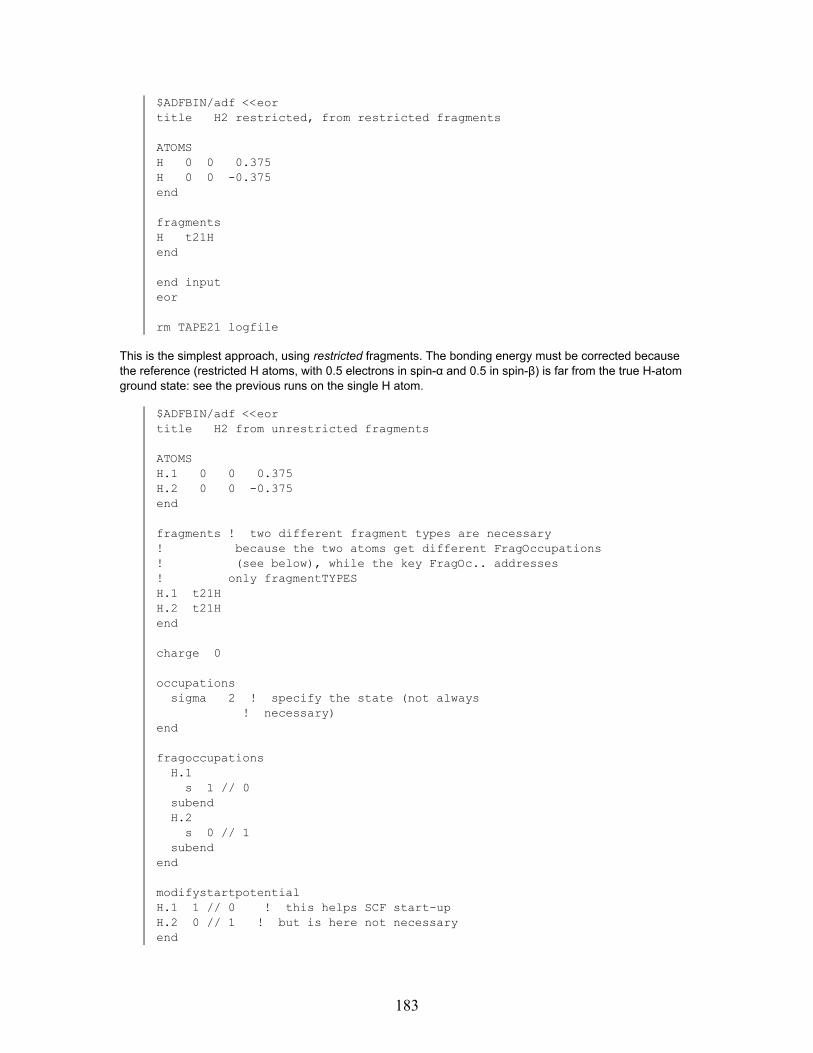
$ADFBIN/adf <<eortitle H2 restricted, from restricted fragments
ATOMSH 0 0 0.375H 0 0 -0.375end
fragmentsH t21Hend
end inputeor
rm TAPE21 logfile
This is the simplest approach, using restricted fragments. The bonding energy must be corrected becausethe reference (restricted H atoms, with 0.5 electrons in spin-α and 0.5 in spin-β) is far from the true H-atomground state: see the previous runs on the single H atom.
$ADFBIN/adf <<eortitle H2 from unrestricted fragments
ATOMSH.1 0 0 0.375H.2 0 0 -0.375end
fragments ! two different fragment types are necessary! because the two atoms get different FragOccupations! (see below), while the key FragOc.. addresses! only fragmentTYPESH.1 t21HH.2 t21Hend
charge 0
occupationssigma 2 ! specify the state (not always
! necessary)end
fragoccupationsH.1
s 1 // 0subendH.2
s 0 // 1subend
end
modifystartpotentialH.1 1 // 0 ! this helps SCF start-upH.2 0 // 1 ! but is here not necessaryend
183

end inputeor
rm TAPE21 logfile
This should be a fair approximation (in the lda model) to the bonding energy of H2 with respect to theunrestricted H atoms. The difference between the bonding energies of this and the previous run should bevery close to the energy of the not-self-consistent unrestricted H-atom with respect to the restricted basicatom (calculation #2).
Excited state
$ADFBIN/adf <<eortitle H2 excited
ATOMSH 0 .0 0.375H 0 .0 -0.375end
fragmentsH t21Hend
fragoccupationsHs 1 // 0subendend
unrestricted
charge 0 2
occupationssigma.g 1 // 0sigma.u 1 // 0end
end inputeor
Finally the calculation of an excited state, with respect to unrestricted fragments. The excitation energy isobtained by comparing the energy with the energy of the ground state calculation. This difference comparesreasonably, but not accurately, to the difference in one-electron ground state energies of the involvedorbitals (Koopman's theorem).
Note that excitation energies can also be calculated with Time-Dependent DFT, using the RESPONSEmodule of ADF. See related sample runs.
PCCP: Bond Energy analysis open-shell fragments
184

Sample directory: adf/PCCP_Unr_BondEnergy/
This example illustrates advanced usage of the bond energy decomposition scheme used in ADF.
A proper decomposition of an electron-pair bond energy requires specifying opposite spins for the unpairedelectrons of the respective radical fragments, which can be done with the input key FragOccupations. Thespecified alpha- and beta-spin configurations of the radical fragments are shown in the output section B U IL D.
Please note that if one neglects explicitly specifying opposite spins for the unpaired electrons of thefragments, each of them is treated as being half an alpha and half a beta electron and consequently, theyenter into a spurious Pauli repulsive interaction. This results, amongst others, into the Pauli repulsion termbeing too repulsive and the orbital interaction term being too much stabilizing.
The example consists of an analysis of the C-C single bond between two CP radicals in the four-atomicmolecule PCCP. The CP fragment calculations used to provide the TAPE21 for the overall PCCP calculationmust be done, for technical reasons, in the restricted mode ("cp_fpccp_asr"). The proper spins are thenspecified in the calculation of the overall molecule using the FragOccupations key ("pccp_fa1_as"). Note thatthis implies a slight approximation because the bond energy computed in this way refers to the energydifference between closed-shell PCCP and two CP radicals that are described by orbitals from a spin-restricted SCF calculation, which have been given an unrestricted occupation. In other words, the set ofalpha- and beta-spin orbitals are identical and the effect of spin polarization is missing. In practice, this leadsto minor energy differences with respect to the correct bond energy, that is, the energy difference betweenclosed-shell PCCP and two CP radicals treated in the unrestricted mode, i.e., for which the set of alpha- andbeta-spin orbitals are allowed to relax toward different solutions in the SCF procedure. This correction termcan be computed directly by carrying out
An unrestricted computation of the CP radical ("cp_fpccp_asu") using the restricted CP radical("cp_fpccp_asr") as a fragment.
$ADFBIN/adf<<eorTITLE cp_fpccp_asr
EPRINTSFO eig ovlEND
XCGRADIENTS BECKE PERDEWEND
ATOMSC .0000 .0000 .6681P .0000 .0000 2.2555
END
FRAGMENTSC t21.CP t21.PEND
integration 5.0
END INPUTeor
mv TAPE21 t21cp_fpccp
185

$ADFBIN/adf<<eorTITLE cp_fpccp_asu
EPRINTSFO eig ovlEND
XCGRADIENTS BECKE PERDEWEND
ATOMSC .0000 .0000 .6681 f=CPP .0000 .0000 2.2555 f=CP
END
FRAGMENTSCP t21cp_fpccpEND
UNRESTRICTEDCHARGE 0 1
integration 5.0
END INPUTeor
rm TAPE21 logfile
$ADFBIN/adf<<eorTITLE pccp_fa1_as
EPRINTSFO eig ovlORBPOP 20 20SUBENDEND
XCGRADIENTS BECKE PERDEWEND
ATOMSP .0000 .0000 2.2555 f=CP_AC .0000 .0000 .6681 f=CP_AC .0000 .0000 -.6681 f=CP_BP .0000 .0000 -2.2555 f=CP_B
END
integration 5.0
FRAGMENTSCP_A t21cp_fpccpCP_B t21cp_fpccpEND
186

SYMMETRY C(LIN)
FRAGOCCUPATIONSCP_A
SIGMA 3//2PI 2//2
SUBENDCP_B
SIGMA 2//3PI 2//2
SUBENDEND
END INPUTeor
TlH: Spin-Orbit SFO analysis
Sample directory: adf/TlH_SO_analysis/
Application of the Spin-Orbit relativistic option (using double-group symmetry) to TlH with a detailed analysisof the spinors in terms of SFOs (Symmetrized Fragment Orbitals).
In order to get the population analysis, one should have one scalar relativistic fragment, which is the wholemolecule. The SFOs in this case are the scalar relativistic orbitals, which are already orthonormal, becauseone has only one fragment which is the whole molecule.
First the relativistic fragment is made, including the create of the atoms:
$ADFBIN/dirac -n1 < $ADFRESOURCES/Dirac/Tl$ADFBIN/dirac -n1 < $ADFRESOURCES/Dirac/Hmv TAPE12 t12.rel
$ADFBIN/adf <<eorcreate Tl file=$ADFRESOURCES/ZORA/TZ2P/Tlxc
LDA vwnGGA becke perdew
endrelativistic scalar zoracorepotentials t12.rel &Tl 1H 2endend inputeormv TAPE21 t21.Tl
$ADFBIN/adf <<eorcreate H file=$ADFRESOURCES/ZORA/TZ2P/Hxc
LDA vwnGGA becke perdew
187

endrelativistic scalar zoracorepotentials t12.rel &Tl 1H 2endend inputeormv TAPE21 t21.H
$ADFBIN/adf <<eortitle TlH, scalar relativistic zora
integration 6.0
relativistic scalar zoracorepotentials t12.rel &Tl 1H 2end
ATOMSTl 0.0 0.0 0.0H 0.0 0.0 1.870end
fragmentsTl t21.TlH t21.Hend
xcLDA vwnGGA becke perdew
end
EPRINTSFO eig ovlEND
end inputeor
mv TAPE21 t21.TlH
In order to get the population analysis, one should have one scalar relativistic fragment, which is the wholemolecule, which is TlH in this case.
$ADFBIN/adf <<eortitle TlH from fragment TlH, with SpinOrbit coupling
integration 6.0
relativistic spinorbit zoracorepotentials t12.rel &Tl 1
188

H 2end
ATOMSTl 0.0 0.0 0.0 f=TlHH 0.0 0.0 1.870 f=TlHend
fragmentsTlH t21.TlHend
xcLDA vwnGGA becke perdew
end
EPRINTSFO eig ovlEND
end inputeor
The output gives something like:
=======================Double group symmetry : *** J1/2 ***=======================
=== J1/2:1 ===
Spinors expanded in SFOs....Spinor: 21 22 23 24occup: 1.00 1.00 1.00 0.00------ ---- ---- ---- ----SFO SIGMA
13.alpha: 0.7614+0.0000i 0.0096+0.0000i 0.0052+0.0000i-0.0006+0.0000i
14.alpha: 0.0154+0.0000i -0.9996+0.0000i 0.0208+0.0000i-0.0077+0.0000i
15.alpha: -0.0146+0.0000i 0.0185+0.0000i 0.9849+0.0000i0.1625+0.0000iSFO PI:x
8.beta : 0.4578+0.0000i 0.0091+0.0000i 0.0112+0.0000i0.0030+0.0000i
9.beta : 0.0005+0.0000i -0.0074+0.0000i -0.1119+0.0000i0.6910+0.0000iSFO PI:y
8.beta : 0.0000+0.4578i 0.0000+0.0091i 0.0000+0.0112i0.0000+0.0030i
9.beta : 0.0000+0.0005i 0.0000-0.0074i 0.0000-0.1119i0.0000+0.6910i....
189

Left out are a lot of small numbers. The meaning is that a spinor of J_z=1/2 symmetry can have SIGMA andPI character, for example, the 21st spinor with occupation number 1.0, is approximately(21 J_z=1/2) = 0.76 (13 SIGMA alpha) + 0.46 (8 PI:x beta) + i 0.46 (8 PI:y beta)
Next in the SFO contributions per spinor the real and imaginary spin alpha part and real and imaginary spinbeta part are all summed together to give a percentage of a certain SFO. are summed. For example the 21stspinor has almost 60% (13 SIGMA) character.
SFO contributions (%) per spinorSpinor: 21 22 23 24occup: 1.00 1.00 1.00 0.00------ ---- ---- ---- ----SFO SIGMA
13: 57.97 0.01 0.00 0.0014: 0.02 99.92 0.04 0.0115: 0.02 0.03 97.01 2.64
SFO PI:x8: 20.96 0.01 0.01 0.009: 0.00 0.01 1.25 47.75
SFO PI:y8: 20.96 0.01 0.01 0.009: 0.00 0.01 1.25 47.75
Bader Analysis (AIM)
Sample directory: adf/Bader/
Starting from the ADF2008.01 version in ADF one calculate Bader atomic charges using a grid basedmethod. This is described in this example. Another possibility for Bader's analysis is to use the adf2aimutility such that a third party program Xaim can be used.
With the BADER input key the ADF program will calculate Bader charges (AIM charges) using a grid basedmethod.
$ADFBIN/adf <<eorTitle Calculate Bader analysis for water
AtomsO 0.000000 0.000000 -0.001658H -0.769048 0.000000 0.595209H 0.769048 0.000000 0.595209
End
BasisType TZPCore none
End
BaderEnd Input
eor
Next a similar calculation for ferrocene is given, which is not repeated here.
190

Bond Orders
Sample directory: adf/BondOrder/
With the key BONDORDER a bond order analysis is performed based on SFOs. Note that symmetry used inthe calculation should be NOSYM. Shown here is only the example for benzene, where the bond orderscalculated are with respect to the atomic fragments.
$ADFBIN/adf <<eortitle benzene BP/SZ bondorders tol=0.05definecc=1.38476576ccc=120.0dih=0.0hc=1.07212846hcc= 120.0dih2=180.0
endatoms Z-matrixC 0 0 0C 1 0 0 ccC 2 1 0 cc cccC 3 2 1 cc ccc dihC 4 3 2 cc ccc dihC 5 4 3 cc ccc dihH 2 1 3 hc hcc dih2H 3 2 4 hc hcc dih2H 4 3 5 hc hcc dih2H 5 4 3 hc hcc dih2H 6 5 4 hc hcc dih2H 1 2 3 hc hcc dih2
endbasisType SZCore None
endsymmetry NOSYMxc
gga becke perdewendbondorder tol=0.05 printallnoprint sfoeor
NOCV: ethylene -- Ni-diimina & H+ -- CO
Sample directories: adf/Diimina_NOCV/ and adf/Hplus_CO_etsnocv
Example for calculation of ETS-NOCV for spin-restricted fragments. ETS-NOCV: energy analysis using theNatural Orbitals for Chemical Valence. The ethylene molecule and a Ni-diimina form a complex together.
191

This example will be discussed first. The other example is H+ and CO form together HCO+, this example issimilar to the discussed example. All electron basis sets are required.
First the two fragments are calculated.
$ADFBIN/adf << eorTitle: et-----Ni-diimina: ethylene runatoms cartesianC -0.430177075 -1.815433265 0.860288229C -0.363705637 -1.910722338 -0.515633302H 0.533109934 -2.284970854 -1.016904201H -1.279922499 -1.884673940 -1.115144723H -1.389295819 -1.753589602 1.377541080H 0.440296224 -2.041861443 1.484489314endbasisType DZPCore Small
endsymmetry NOSYMxcgga scf becke perdew
endendinputeormv TAPE21 t21.etfrag
$ADFBIN/adf << eorTitle: et-----Ni-diimina: Ni-diimina runatoms cartesianNi 0.022615419 0.037783871 0.025751533N 0.386170317 1.871072585 0.306265538C 1.612863056 2.248007643 0.148716016C 2.540686607 1.163409862 -0.183603690N 1.976290003 0.008161589 -0.301176178H -0.288333328 2.609667211 0.546869047H 1.942601454 3.283060847 0.269249237H 3.613259273 1.338293482 -0.302134814H 2.621707427 -0.766258151 -0.517479818H -1.351756655 0.253389698 0.386197419endcharge 1basisType DZPCore Small
endsymmetry NOSYMxc
gga scf becke perdewendendinputeormv TAPE21 t21.Nifrag
Next these fragments are used in the calculation of the full complex. The keys ETSNOCV and 'PRINTetslowdin' are needed in this case to to analyze the bonding in the molecule with respect to the fragments.The symmetry must be NOSYM.
192

$ADFBIN/adf << eorTitle: et-----Ni-diimina runatomsNi 0.022615419 0.037783871 0.025751533 f=kN 0.386170317 1.871072585 0.306265538 f=kC 1.612863056 2.248007643 0.148716016 f=kC 2.540686607 1.163409862 -0.183603690 f=kN 1.976290003 0.008161589 -0.301176178 f=kH -0.288333328 2.609667211 0.546869047 f=kH 1.942601454 3.283060847 0.269249237 f=kH 3.613259273 1.338293482 -0.302134814 f=kH 2.621707427 -0.766258151 -0.517479818 f=kH -1.351756655 0.253389698 0.386197419 f=kC -0.430177075 -1.815433265 0.860288229 f=mC -0.363705637 -1.910722338 -0.515633302 f=mH 0.533109934 -2.284970854 -1.016904201 f=mH -1.279922499 -1.884673940 -1.115144723 f=mH -1.389295819 -1.753589602 1.377541080 f=mH 0.440296224 -2.041861443 1.484489314 f=mendcharge 1fragmentsm t21.etfragk t21.Nifragendsymmetry NOSYMxcgga scf becke perdew
endETSNOCVprint etslowdinendinputeor
Next one could do densf calculations, to view the natural orbitals in this method, see also the thedocumentation for the densf analysis program and the ADF-GUI. Input is the TAPE21 of the molecularcalculation.
$ADFBIN/densf << eorGRID MEDIUMNOCV
THRESH 0.01ENDEND INPUTeormv TAPE41 nocv2.t41
$ADFBIN/densf << eorGRID MEDIUMNOCV
ALLENDEND INPUTeormv TAPE41 nocv3.t41
193

NOCV: CH2 -- Cr(CO)5
Sample directory: adf/NOCV_CrCO5-CH2/
Example for calculation of ETS-NOCV for spin-restricted fragments. ETS-NOCV: energy analysis using theNatural Orbitals for Chemical Valence. The CH2 molecule and Cr(CO)5 are the fragments, which formCr(CO)5CH2 molecule.
First the two fragments are calculated.
$ADFBIN/adf -n1 << eorTitle CrCO5--[CH2] run from CrCO5 and CH2 closed shell fragments,FULLelectron calc.!atoms cartesian
C -0.429104 1.732058 -0.225052H 0.407023 2.440417 -0.352323H -1.385325 2.281354 -0.254124
endbasisType DZPCore None
endsymmetry NOSYMxc
gga becke perdewendendinputeormv TAPE21 t21.CH2
$ADFBIN/adf -n1 << eorTitle [CrCO5] runatoms cartesian
Cr -0.248053 -0.169062 0.005810C -0.072963 -2.080685 0.229583O 0.030811 -3.223220 0.361925C -0.182894 0.049840 1.909128O -0.142780 0.212309 3.050403C -0.299940 -0.409118 -1.894730O -0.331795 -0.521589 -3.042336C -2.138631 -0.242152 0.075713O -3.295036 -0.249916 0.115045C 1.624487 0.092244 -0.083118O 2.763411 0.288575 -0.140976
endbasisType DZPCore NoneCr $ADFRESOURCES/TZP/Cr
endsymmetry NOSYMxc
gga becke perdew
194

endendinputeormv TAPE21 t21.Crfragment
Next these fragments are used in the calculation of the full complex. The keys ETSNOCV and 'PRINTetslowdin' are needed in this case to to analyze the bonding in the molecule with respect to the fragments.The symmetry must be NOSYM. Note the '-n1' flag for adf: this enforces that a single-node (non-parallel) runis performed.
$ADFBIN/adf -n1 << eorTitle:CrCO5--[CH2], etsnocv activated by etsnocv and print etslowdinatoms
C -0.429104 1.732058 -0.225052 f=f1Cr -0.248053 -0.169062 0.005810 f=f2C -0.072963 -2.080685 0.229583 f=f2O 0.030811 -3.223220 0.361925 f=f2C -0.182894 0.049840 1.909128 f=f2O -0.142780 0.212309 3.050403 f=f2C -0.299940 -0.409118 -1.894730 f=f2O -0.331795 -0.521589 -3.042336 f=f2C -2.138631 -0.242152 0.075713 f=f2O -3.295036 -0.249916 0.115045 f=f2C 1.624487 0.092244 -0.083118 f=f2O 2.763411 0.288575 -0.140976 f=f2H 0.407023 2.440417 -0.352323 f=f1H -1.385325 2.281354 -0.254124 f=f1
endfragmentsf1 t21.CH2f2 t21.Crfragmentendsymmetry NOSYMxc
gga becke perdewendETSNOCV RHOKMIN=1.e-3 EKMIN=1.5 ENOCV=0.05print etslowdinendinputeor
NOCV: CH3 -- CH3
Sample directory: adf/CH3_CH3_etsnocv/
Example for calculation of ETS-NOCV for unrestricted fragments. ETS-NOCV: energy analysis using theNatural Orbitals for Chemical Valence. The ethane molecule is built from two methyl radicals
First the two methyl fragments are calculated. The fragments should be spin-restricted.
$ADFBIN/adf << eorTitle CH3-CH3 built from CH3 radicals, FULL electron calc.!atoms cartesian
C 0.019664 -0.034069 0.009101
195

H 0.039672 -0.069395 1.109620H 1.063205 -0.065727 -0.341092H -0.474230 -0.953693 -0.341621
endbasisH $ADFRESOURCES/DZP/HC $ADFRESOURCES/DZP/Cendsymmetry NOSYMSCF
Iterations 2500Converge 1E-6
endxc
gga scf becke perdewendendinputmv TAPE21 t21.frag1
$ADFBIN/adf << eorTitle CH3 radicalatoms cartesian
C -0.703210 1.217999 -0.497874H -0.723753 1.252869 -1.598316H -1.746567 1.250049 -0.147169H -0.208833 2.137544 -0.147653
endbasisH $ADFRESOURCES/DZP/HC $ADFRESOURCES/DZP/Cendsymmetry NOSYMSCF
Iterations 2500Converge 1E-6
endxc
gga scf becke perdewendendinputeormv TAPE21 t21.frag2
Next these fragments are used in the calculation of the molecule ethane, using the keyFRAGOCCUPATIONS to use an unrestricted fragment occupation for the methyl radicals, such that they areprepared for bonding. In the one fragment the singly occupied orbital will be an α-orbital, and in the otherfragment the singly occupied orbital will be a β-orbital, such that the calculated Pauli repulsion between thefragments will be small.
The keys ETSNOCV and 'PRINT etslowdin-unrestricted' are needed in this case to to analyze the bonding ina molecule with unpaired electrons in the fragments. The symmetry must be NOSYM.
$ADFBIN/adf << eorTitle: final [CH3]-[CH3], etsnocv activated by etsnocv andetslowdin-unrestrictedatoms
C 0.019664 -0.034069 0.009101 f=f1
196

H 0.039672 -0.069395 1.109620 f=f1H 1.063205 -0.065727 -0.341092 f=f1H -0.474230 -0.953693 -0.341621 f=f1C -0.703210 1.217999 -0.497874 f=f2H -0.723753 1.252869 -1.598316 f=f2H -1.746567 1.250049 -0.147169 f=f2H -0.208833 2.137544 -0.147653 f=f2
endfragmentsf1 t21.frag1f2 t21.frag2
endfragoccupationsf1A 5 // 4
subendf2A 4 // 5
subendendsymmetry NOSYMSCF
Iterations 800Converge 1E-6
endxc
gga scf becke perdewendETSNOCV RHOKMIN=1.e-3 EKMIN=1.5 ENOCV=0.05PRINT etslowdin-unrestrictedend inputeor
Next 2 densf calculations, to view the natural orbitals in this method, see also the the documentation for thedensf analysis program and the ADF-GUI. Input is the TAPE21 of the molecular calculation.
$ADFBIN/densf << eorGRID MEDIUMNOCVAlpha125960
Beta125960
ENDEND INPUTeormv TAPE41 nocv1.t41$ADFBIN/densf << eorGRID MEDIUMNOCV
THRESH 0.01
197

ENDEND INPUTeormv TAPE41 nocv2.t41eor
Post-ADF analysis utilities
NO2: Contour Plots using Densf and Cntrs
Sample directory: adf/Cntrs_NO2/
This example illustrates using the utility programs cntrs and densf. See the Utilities document for details.
$ADFBIN/adf << eortitle NO2
atomsN 0 0 0O 1.009356 0 0.464189O -1.009356 0 0.464189end
BasisType DZCore Small
End
unrestrictedcharge 0 1
endinputeor
After the normal ADF calculation on NO2 has been completed, the utility program densf is executed togenerate a TAPE41 file with user-specified items evaluated in a regular, user-specified grid.
The TAPE21 on which densf operates must be present as a local file with name TAPE21.
$ADFBIN/densf << eordensity scf ortho fragfitdensity scf ortho fragorbitals scfalphaa1 1 2a2 1b1 2betaa2 1b1 1 2b2 1endcoulpot frag ortho scf
198

grid-7.5 -7.5 0.0
51 511.0 0.0 0.0 15.000.0 1.0 0.0 15.00endend inputeor
The charge density values in the grid are requested for all available types of density: exact and fitted, for theinitial (sum-of-fragments), intermediate (orthogonalized fragments, see the ADF User's Guide) and final(SCF) situation.
Several SCF molecular orbitals are computed by specifying their indices in the energy-ordered list (aseparate list for each symmetry subspecies).
The coulomb potentials (again: for sum-of-fragments, orthogonalized fragments, and SCF) are generated.
The grid is defined by an 'origin', the numbers of points in all independent grid directions and the directionvectors with the total grid size in each direction separately.
Since there are only two 'numbers-of-points' (51 each) a 2-dimensional grid is generated. 1D and 3D gridsare also possible. See the Utilities document for a more detailed survey of the available options.
The result of the densf run is a file tape41 (binary, KF). This contains all computed data. tape41 can be usedby cntrs to generate plot data.
$ADFBIN/cntrs << eorscan0.02 0.05 0.10 0.2 0.5 0.0 -.02 -.05 -.10 -.2 -.5enddash 0.2file cont.dSCF%Density_ASCF%Density_Bendinputeor
In this example eleven (11) scan values are defined to draw contours for, with a dash length of 0.2 bohr.
An ascii file cont.d will be opened by cntrs on which the specified items (SCF-densities for spin-up and spin-down) will be combined (by default: simply added) into one quantity.
For this quantity the contour lines that correspond to the specified scan values are stored. See the Utilitiesdocument for precise specifications and options.
gnuplot << eor
set term dumb 100 80set output "outplot"plot "cont.d" using 1:2 with lineseor
cat outplot
The public domain software gnuplot (not included in the adf package) is applied here to display the resultfrom cntrs. The resulting picture on your screen (if you have gnuplot available) looks like
199

10 *+** ************************ ***** ****** ** ************ *** ** ********* ******** ********** *** ** ** *********** **** ********** ** ** * ***** *** **** **** ** * * * ********** ********** **** *
8 *+ * * * ** ******* * * *** * * * ** ** * * ** * * * * * **** * * * ** * * * * ** * * * * *** ** ** * * * * * **** * * * ** ** ** ** * ** * * ** * * * ** ******* * * ** ** * * ********** ********** **** *
* * ** *** ********* ****** *** ** ** ********* ********* ** *
6 *+ ** *********** ****** ********** *** *** ********** **** ********** *********** ***********
C2H2: Localization of Molecular Orbitals
Sample directory: adf/Cntrs.LocOrb_C2H2/
An illustration of the computation of localized molecular orbitals in C2H2.
The delocalized molecular orbitals as they result from the scf are localized in two different ways. In the firstthe three σ bonds are recombined only among themselves (no π bonds are mixed in), yielding twoequivalent localized CH σ bonds and one localized σ bond. In a second step the localization of theremaining bond (the two π's) is performed, but this produces nothing new since no combination of the twoπ's is more localized then they are already by themselves.
$ADFBIN/adf << eortitle C2H2, localization Sigma and Pi separately
AtomsC 0 0 .63C 0 0 -.63H 0 0 1.63H 0 0 -1.63END
BasisType TZPCore Small
End
LocOrbalfa 4 5alfa 1 2 3
200

END
integration 4.0
end inputeor
In the first localization cycle the π-orbitals are left out: #4 and #5 in the list of all occupied valence MOs: first3 MOs of the first irreducible representation (s), then the 2 from the second irrep (π). In the secondlocalization step the first three (meanwhile localized) orbitals are kept aside.
With densf the local orbitals can be computed in a user-defined grid (for plotting purposes). densf requires afile with name TAPE21.
$ADFBIN/densf << eor
Grid0. -5. -5.100 1000. 0. 1. 10.0. 1. 0. 10.
End
Orbitals Local1 2 3 4 5
End
END INPUTeor
The program cntrs is applied to process the densf result file TAPE41.
$ADFBIN/cntrs << eor
SCAN0.01 0.02 0.04 0.08 0.16 0.32 0.64 1.28-0.01 -0.02 -0.04 -0.08 -0.16 -0.32 -0.64 -1.28
END
file ctr.a1LocOrb%1 1.00
file ctr.a2LocOrb%2 1.00
file ctr.a3LocOrb%3 1.00
file ctr.a4LocOrb%4 1.00
file ctr.a5LocOrb%5 1.00
END INPUTeor
Again, gnuplot may be used to display the result on your screen.
201

$gnuplot << eorset term dumb 100 80set output "outplot"plot "ctr.a1" using 1:2 with linesplot "ctr.a2" using 1:2 with linesplot "ctr.a3" using 1:2 with linesplot "ctr.a4" using 1:2 with linesplot "ctr.a5" using 1:2 with lineseor
cat outplot
This results in 5 pictures, the first one looking like:
******************** ****
*** ***** ***** ***** **
** *** *** **** *** *** **
** ** ********** *** ** **** **** **
** * *** *** * *** ** ** ** ** ** * *** ********** *** * ** * * *** *** * * ** * ** ** ** ** * *
***** * * * * * * * *** ** * * * * ******** * * * *
* ** * * * ** **** **** ** * * ** * *** * * *** *** * * ***
** **** * ***** * ** ** * ****** *** **** ** **** * * * * **** *
** ** ****** ****** * * ****** ****** * * *********** ************ *************
** * ** ********* ** ** *********** * ** *** ** ******** * * ******** *** ** * ** ** * ********* ********* * ** ** * * *** ** *** ***** ****** ** * *** * * *** * * ******* ****** ** ** *** * * * ** * ********* ********* * ** ** * ** *** ** ******** * * ******** **** * ** ********** ** ** *********** * ************ ************ *************** ** ***** ****** * * ****** ******
* ***** * ***** * ** ** * ***** *** ** *** * * *** *** * * ***
* ** * * * ** **** **** ** * * **** ** * * * * ******** * * * *
***** * * * * * * * ** * ** ** ** ** * ** * * *** *** * * ** * *** ********** *** * ** ** ** ** ** *** * *** *** * **
202

* ** **** **** ** *** ** ********** ** **** *** *** **** *** *** **** ***** ***** **
** ********** ***** ***
**** ********************
The second illustration of the computation of localized molecular orbitals in C2H2 combines directly all MOs(σ and π). This yields 3 equivalent 'banana' bonds, mixtures of σ and π, and two equivalent pure σ bonds.
$ADFBIN/adf << eortitle C2H2 localization without frozen orbitals
AtomsC 0 0 .63C 0 0 -.63H 0 0 1.63H 0 0 -1.63end
fragmentsC t21.CH t21.Hend
integration 4.0
locorbend
end inputeor
Cu4CO: Density of States
Sample directory: adf/DOS_Cu4CO/
This sample illustrates the DOS property program to compute density-of-states data, for energy-dependentanalysis.
First, the Cu4CO molecule is calculated (ADF), using single-atom fragments.
$ADFBIN/adf <<eortitle Cu4CO (3,1) from atoms
unitslength bohrend
203
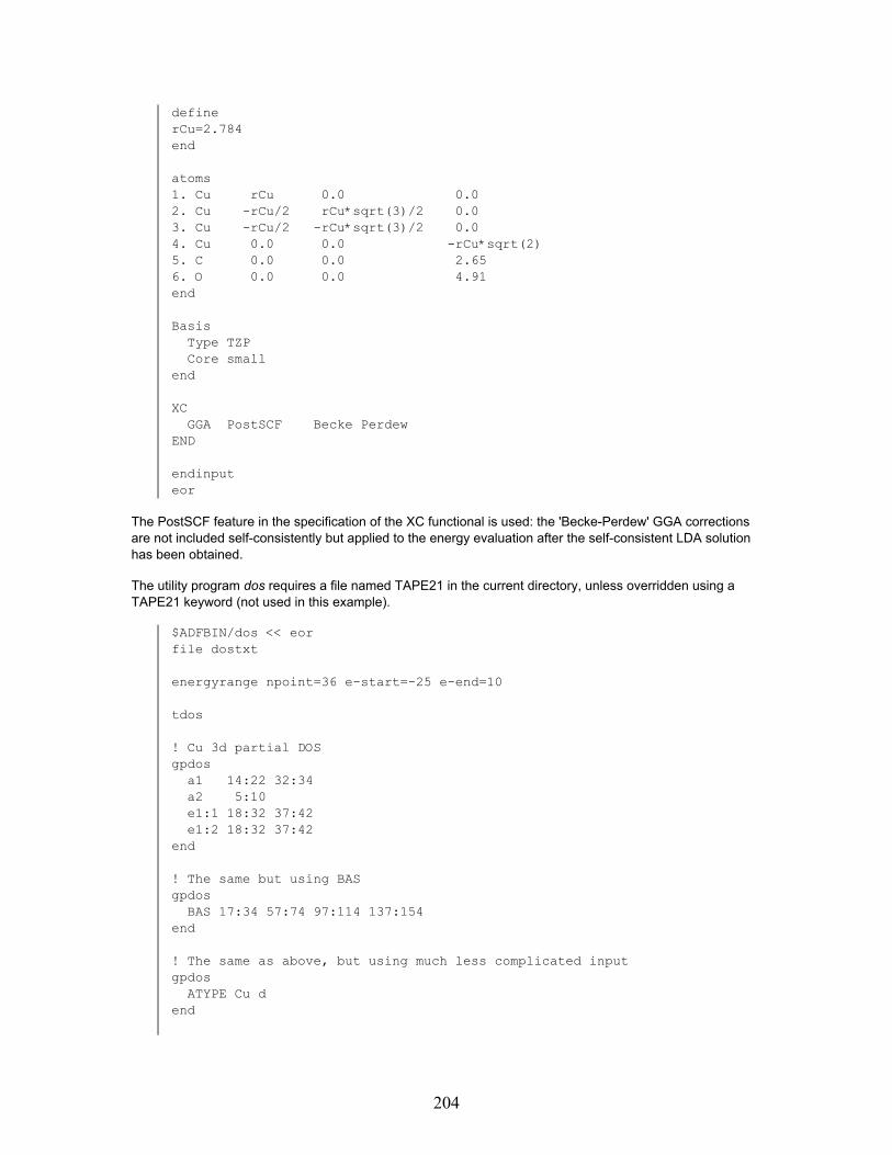
definerCu=2.784end
atoms1. Cu rCu 0.0 0.02. Cu -rCu/2 rCu*sqrt(3)/2 0.03. Cu -rCu/2 -rCu*sqrt(3)/2 0.04. Cu 0.0 0.0 -rCu*sqrt(2)5. C 0.0 0.0 2.656. O 0.0 0.0 4.91end
BasisType TZPCore small
end
XCGGA PostSCF Becke Perdew
END
endinputeor
The PostSCF feature in the specification of the XC functional is used: the 'Becke-Perdew' GGA correctionsare not included self-consistently but applied to the energy evaluation after the self-consistent LDA solutionhas been obtained.
The utility program dos requires a file named TAPE21 in the current directory, unless overridden using aTAPE21 keyword (not used in this example).
$ADFBIN/dos << eorfile dostxt
energyrange npoint=36 e-start=-25 e-end=10
tdos
! Cu 3d partial DOSgpdos
a1 14:22 32:34a2 5:10e1:1 18:32 37:42e1:2 18:32 37:42
end
! The same but using BASgpdos
BAS 17:34 57:74 97:114 137:154end
! The same as above, but using much less complicated inputgpdos
ATYPE Cu dend
204

! Overlap PDOS between Cu 3d and CO 2popdos
ATYPE Cu 3dSUBEND
ATOM 5 2pATOM 6 2p
end
end inputeor
Here, the total density of states, as well as various partial densities of states, are computed. You may feedthe results found in the dostxt file into a plotting program such as gnuplot. The result is not displayed here.See the Utilities document for more detailed info about the dos program.
Charge transfer integrals (transport properties)
AT base pair: Charge transfer integrals
Sample directory: adf/AT_transferintegrals/
ADF can can calculate charge transfer integrals, that are needed in approximate methods that model chargetransport properties. The molecular system typically should be build from 2 fragments. In this examplecharge transfer integrals are calculated between Adenine and Thymine. First these two molecules arecalculated. In the fragment calculation full symmetry can be used.
$ADFBIN/adf <<eorTITLE Adenine fragmentATOMS1 N 0.000000000000 0.656191000000 4.4734500000002 C 0.000000000000 1.850911000000 5.0988500000003 N 0.000000000000 2.094911000000 6.4110700000004 C 0.000000000000 0.951291000000 7.1150100000005 C 0.000000000000 -0.355699000000 6.6117400000006 C 0.000000000000 -0.487619000000 5.2033300000007 N 0.000000000000 0.791131000000 8.4843500000008 C 0.000000000000 -0.567649000000 8.7292900000009 N 0.000000000000 -1.292469000000 7.63145000000010 N 0.000000000000 -1.672349000000 4.57261000000011 H 0.000000000000 2.715551000000 4.43392000000012 H 0.000000000000 1.540301000000 9.16615000000013 H 0.000000000000 -0.961519000000 9.73982000000014 H 0.000000000000 -2.515699000000 5.12990000000015 H 0.000000000000 -1.718459000000 3.541030000000ENDBASIStype DZcore NoneENDeormv TAPE21 Adenine.t21
$ADFBIN/adf <<eor
205

TITLE Thymine fragmentATOMS1 N 0.000000000000 0.617991000000 1.6660400000002 C 0.000000000000 1.851251000000 1.0462600000003 N 0.000000000000 1.768641000000 -0.3473800000004 C 0.000000000000 0.582611000000 -1.0421600000005 C 0.000000000000 -0.621999000000 -0.4170400000006 C 0.000000000000 -0.627269000000 1.0458800000007 O 0.000000000000 -1.670479000000 1.7207800000008 O 0.000000000000 2.924531000000 1.6366000000009 C 0.000000000000 -1.937039000000 -1.13813000000010 H 0.000000000000 0.635221000000 2.73338000000011 H 0.000000000000 2.660141000000 -0.83010000000012 H 0.000000000000 0.676731000000 -2.12710000000013 H 0.880180000000 -2.533409000000 -0.86065000000014 H 0.000000000000 -1.793509000000 -2.22578000000015 H -0.880180000000 -2.533409000000 -0.860650000000ENDBASIStype DZcore NoneENDeormv TAPE21 Thymine.t21
Next the the base pair is calculated that consists of Adenine and Thymine. To calculate the charge transferintegrals, spatial overlap integrals and site energies, include the key TRANSFERINTEGRALS in the input forADF. Symmetry NOSYM should be used.
$ADFBIN/adf <<eorTITLE ATATOMS1 N 0.000000000000 0.656191000000 4.473450000000f=Adenine2 C 0.000000000000 1.850911000000 5.098850000000f=Adenine3 N 0.000000000000 2.094911000000 6.411070000000f=Adenine4 C 0.000000000000 0.951291000000 7.115010000000f=Adenine5 C 0.000000000000 -0.355699000000 6.611740000000f=Adenine6 C 0.000000000000 -0.487619000000 5.203330000000f=Adenine7 N 0.000000000000 0.791131000000 8.484350000000f=Adenine8 C 0.000000000000 -0.567649000000 8.729290000000f=Adenine9 N 0.000000000000 -1.292469000000 7.631450000000f=Adenine10 N 0.000000000000 -1.672349000000 4.572610000000f=Adenine11 H 0.000000000000 2.715551000000 4.433920000000f=Adenine12 H 0.000000000000 1.540301000000 9.166150000000f=Adenine13 H 0.000000000000 -0.961519000000 9.739820000000
206

f=Adenine14 H 0.000000000000 -2.515699000000 5.129900000000f=Adenine15 H 0.000000000000 -1.718459000000 3.541030000000f=Adenine16 N 0.000000000000 0.617991000000 1.666040000000f=Thymine17 C 0.000000000000 1.851251000000 1.046260000000f=Thymine18 N 0.000000000000 1.768641000000 -0.347380000000f=Thymine19 C 0.000000000000 0.582611000000 -1.042160000000f=Thymine20 C 0.000000000000 -0.621999000000 -0.417040000000f=Thymine21 C 0.000000000000 -0.627269000000 1.045880000000f=Thymine22 O 0.000000000000 -1.670479000000 1.720780000000f=Thymine23 O 0.000000000000 2.924531000000 1.636600000000f=Thymine24 C 0.000000000000 -1.937039000000 -1.138130000000f=Thymine25 H 0.000000000000 0.635221000000 2.733380000000f=Thymine26 H 0.000000000000 2.660141000000 -0.830100000000f=Thymine27 H 0.000000000000 0.676731000000 -2.127100000000f=Thymine28 H 0.880180000000 -2.533409000000 -0.860650000000f=Thymine29 H 0.000000000000 -1.793509000000 -2.225780000000f=Thymine30 H -0.880180000000 -2.533409000000 -0.860650000000f=ThymineENDFragments
Adenine Adenine.t21Thymine Thymine.t21
endSYMMETRY NOSYMTRANSFERINTEGRALSeor
After the calculation has finished in the output one will find the charge transfer (overlap integrals and siteenergies) that are needed to calculate hole mobility or electron mobility calculations.
Overlap integral (hole) HOMO fragment 1 - HOMO fragment 2: 0.00000Site energy (hole) HOMO fragment 1 (eV): -6.89282Site energy (hole) HOMO fragment 2 (eV): -6.49009Charge transfer integral (hole) HOMO fragment 1 - HOMO fragment 2
(eV): 0.00000
Overlap integral (electron) LUMO fragment 1 - LUMO fragment 2:0.00396Site energy (electron) LUMO fragment 1 (eV): -2.23423Site energy (electron) LUMO fragment 2 (eV): -2.64264
207

Charge transfer integral (electron) LUMO fragment 1 - LUMO fragment 2(eV): -0.04543
Third party analysis software
adf2aim: convert an ADF TAPE21 to WFN format (for Bader analysis)
Sample directory: adf/AIM_HF/
Starting from the ADF2008.01 version in ADF one calculate Bader atomic charges using a grid basedmethod. Another possibility for Bader's analysis, an example is described here, is to use the adf2aim utilitysuch that a third party program Xaim can be used.
ADF utility adf2aim (original name rdt21) developed by Xavi López, Engelber Sans and Carles Bo (seehttp://www.quimica.urv.es/ADF_UTIL):rdt21: convert an ADF TAPE21 to WFN format (for Bader analysis)This program rdt21 is now called adf2aim and is part of the ADF package, starting from ADF2004.01.
The WFN file is an input file for the third party program Xaim (see http://www.quimica.urv.es/XAIM fordetails), which is a graphical user interface to programs that can perform the Bader analysis.
Usage of adf2aim:
$ADFBIN/adf <<eorTITLE HF
ATOMS1. H .0000 .0000 .00002. F .0000 .0000 0.917
End
BasisEnd
End inputeor
$ADFBIN/adf2aim TAPE21echo 'Contents of rdt21.res:'cat rdt21.resecho 'Contents of WFN:'cat WFN
NBO analysis: adfnbo, gennbo
Sample directory: adf/H2O_ADFNBO/
Dr. Autschbach, SCM, and Prof. Weinhold have collaborated to prepare a simple in put file generator, calledadfnbo, for the GENNBO program of Prof. Weinholds Natural Bond Orbital (NBO) 5.0 package:http://www.chem.wisc.edu/~nbo5
208

The GENNBO executable is included in the ADF distribution and can be enabled via the license file for allthose who buy an NBO manual from either the NBO authors or from SCM ([email protected]).
Usage:
$ADFBIN/adf <<eorTitle simple NBO example for water
Atoms Z-MatrixO 0 0 0H 1 0 0 0.9H 1 2 0 0.9 100End
BasisCORE NONETYPE DZEnd
FULLFOCKAOMAT2FILESAVE TAPE15SYMMETRY NOSYM
End Inputeor
$ADFBIN/adfnbo <<eorwritefocksphericalend inputeor
$ADFBIN/gennbo < FILE47
Note added: recommended is to use the key 'spherical' in the adfnbo input.
A File named FILE47 is generated by adfnbo which is an input file for the general NBO program gennbo.ADF needs to write some data to file, which is done by including these keywords in the adf input file:
FULLFOCKAOMAT2FILESAVE TAPE15SYMMETRY NOSYM
GENNBO
This section contains a brief summary of the capabilities of GENNBO, made available by Prof. Weinhold.
GENNBO implements most capabilities of the full NBO 5.0 program suite as described on the NBO website:http://www.chem.wisc.edu/~nbo5These include determination of natural atomic orbitals (NAOs), bond orbitals (NBOs), and localized MOs(NLMOs), as well as the associated NPA (atomic charges and orbital populations) and NRT (resonancestructures, weightings, bond orders) valence descriptors, for a wide variety of uncorrelated and correlated(variational, perturbative, or density functional) theoretical levels. GENNBO-supported options include all
209

keywords except those explicitly requiring interactive communication with the host electronic structuresystem (viz., $DEL deletions, NEDA, NCS, NJC). The GENNBO program typically sits conveniently on thePC desktop, ready to analyze (or re-analyze at will, with altered options) the final results of a complex ADFcalculation performed on a remote cluster.
GENNBO "communicates" with the original ADF calculation through an archive file (JOB.47 file, preservingall necessary details of the final density) that is initially generated by ADF and subsequently becomes theinput file for GENNBO. The .47 file contains a standard $NBO ... $END keylist that can be edited with astandard word processor or text editor to include chosen NBO keyword options, just as though they mighthave appeared in the original input stream of an interactive ADFNBO run. The stand-alone GENNBOprogram therefore allows many alternative NBO analysis options to be explored at leisure, without costly re-calculation of the wavefunction.
NBO analysis: EFG
Sample directory: adf/AlCl3_efgnbo/
Example shows an NBO analysis of an EFG calculation for AlCl3.
In the ADF input one then needs to include the QTENS (EFG calculation) and include the subkey EFG of thekey AORESPONSE. A higher integration accuracy in the core region is used (subkey ACCSPH of the keyINTEGRATION). Other keywords are necessary because of the NBO analysis afterwards. Note that ADF,ADFNBO, and GENNBO have to run several times.
$ADFBIN/adf << eorTitle AlCl3atomsAl 0.000000 0.000000 -0.237368Cl 1.808813 0.000000 0.807083Cl 0.000000 0.000000 -2.326083Cl -1.808813 0.000000 0.807083
Endxclda vwngga revPBE
endSymmetry NOSYMIntegrationaccint 4.5accsph 5.5
EndAoresponseefg 1 nbo
endqtenssave TAPE15FULLFOCKAOMAT2FILEEND INPUTeor
$ADFBIN/adfnbo << eorwritespherical
210

fockTESTJOBend inputeor
rm -f adfnbo.37 adfnbo.39 adfnbo.49 adfnbo.48
$ADFBIN/gennbo < FILE47
$ADFBIN/adfnbo << eorcopysphericalfock
TESTJOBend inputeor
$ADFBIN/adfnbo << eorreadsphericalfock
TESTJOBend inputeor
rm -f adfnbo.37 adfnbo.39 adfnbo.49 adfnbo.48
rm -f TAPE21 TAPE13 TAPE15
$ADFBIN/adf << eorTitle AlCl3atomsAl 0.000000 0.000000 -0.237368Cl 1.808813 0.000000 0.807083Cl 0.000000 0.000000 -2.326083Cl -1.808813 0.000000 0.807083
Endxclda vwngga revPBE
endSymmetry NOSYMIntegrationaccint 4.5accsph 5.5
EndBasisType TZPCore none
EndAoresponseefg 1 nbo
endqtensEnd Inputeor
211

NBO analysis: NMR chemical shift
Sample directory: adf/CH4_nmrnbo/
Example shows an NBO analysis of an NMR shielding calculation for CH4.
Some keywords are necessary because of the NBO analysis afterwards. A higher integration accuracy inthe core region is used (subkey ACCSPH of the key INTEGRATION). First the scalar relativistic calculationis performed and the scalar relativistic localized orbitals are made. Next the spin-orbit coupled ADFcalculation is done, and a calculation of NMR shielding constants is performed with an analyisis in scalarrelativistic localized orbitals.
$ADFBIN/adf << eorATOMSC 0.0000 0.0000 0.0000H 0.6316 0.6316 0.6316H 0.6316 -0.6316 -0.6316H -0.6316 0.6316 -0.6316H -0.6316 -0.6316 0.6316
ENDsave TAPE15FULLFOCKAOMAT2FILEBASIStype DZPcore None
ENDINTEGRATIONaccint 4.5accsph 5.5
endrelativistic scalar zoraeor
$ADFBIN/adfnbo << eorwritesphericalfockTESTJOBend inputeor
rm adfnbo.37 adfnbo.39 adfnbo.49 adfnbo.48
$ADFBIN/gennbo < FILE47
$ADFBIN/adfnbo << eorcopysphericalfock
end inputeor
rm adfnbo.37 adfnbo.39 adfnbo.49 adfnbo.48
212

rm TAPE15 TAPE21 logfile
$ADFBIN/adf << eorATOMSC 0.0000 0.0000 0.0000H 0.6316 0.6316 0.6316H 0.6316 -0.6316 -0.6316H -0.6316 0.6316 -0.6316H -0.6316 -0.6316 0.6316
ENDBASIStype DZPcore None
ENDSYMMETRY nosymINTEGRATIONaccint 4.5accsph 5.5
endrelativistic spinorbit zoraend inputeor
rm TAPE15 TAPE10 logfile SINFO IINFO
$ADFBIN/nmr << eornoscale
nmratoms 2 1u1k bestcalc all :: nosclout iso tens
endanalysisprint 0.01canonicalnbocomponents
endend inputeor
NBO analysis: NMR spin-spin coupling
Sample directory: adf/CPL_CH3OH_NBO/
Example shows an NBO analysis of an NMR spin-spin coupling constants calculation for CH3OH.
Some keywords are necessary because of the NBO analysis afterwards. A higher integration accuracy inthe core region is used (subkey ACCSPH of the key INTEGRATION). First the scalar relativistic calculationis performed and the scalar relativistic localized orbitals are made, and a calculation of NMR spin-spincoupling constants is performed with an analyisis in scalar relativistic localized orbitals. Next the spin-orbit
213

coupled ADF calculation is done, and a calculation of NMR spin-spin coupling constants is performed withan analyisis in scalar relativistic localized orbitals.
$ADFBIN/adf << eorATOMS1 O 0.151078120000 -0.158942890000 -0.1843820100002 H 0.762854510000 0.480823600000 0.1878678300003 C 0.654254930000 -1.481762230000 0.0263436300004 H 1.616760580000 -1.581906770000 -0.4556708000005 H -0.035909520000 -2.200223490000 -0.3934339600006 H 0.761359880000 -1.661537720000 1.087000640000
ENDsave TAPE15FULLFOCKAOMAT2FILEBASIStype DZPcore None
ENDSCFconverge 1.0e-8
ENDSYMMETRY nosymINTEGRATIONaccint 4.5accsph 5.5
endrelativistic scalar zoraend inputeor
$ADFBIN/adfnbo << eorwritesphericalfockTESTJOBend inputeor
rm adfnbo.37 adfnbo.39 adfnbo.49 adfnbo.48
$ADFBIN/gennbo < FILE47
$ADFBIN/adfnbo << eorcopysphericalfock
end inputeor
$ADFBIN/adfnbo << eorsphericalfockread
end inputeor
214

rm adfnbo.37 adfnbo.39 adfnbo.49 adfnbo.48rm TAPE15 TAPE21 TAPE13 logfile
$ADFBIN/cpl << eornmrcouplingxalphadsopsosdscf convergence 1e-5 iterations 10contributions 1e19 nbonuclei 3 5 6
endendinputeor
rm TAPE15 TAPE21 TAPE13 logfile
$ADFBIN/adf << eorATOMS1 O 0.151078120000 -0.158942890000 -0.1843820100002 H 0.762854510000 0.480823600000 0.1878678300003 C 0.654254930000 -1.481762230000 0.0263436300004 H 1.616760580000 -1.581906770000 -0.4556708000005 H -0.035909520000 -2.200223490000 -0.3934339600006 H 0.761359880000 -1.661537720000 1.087000640000
ENDBASIStype DZPcore None
ENDSYMMETRY nosymSCFconverge 1.0e-8
ENDINTEGRATIONaccint 4.5accsph 5.5
endrelativistic spinorbit zoraend inputeor
rm TAPE15
$ADFBIN/cpl << eornmrcouplingxalphadsopsosdscf convergence 1e-5 iterations 10contributions 1e19 nbonuclei 3 5 6
endend inputeor
215

Accuracy
BSSE, SCF convergence, Frequencies
Cr(CO)5+CO: Basis Set Superposition Error
Sample directory: adf/BSSE_CrCO6/
A study of the Basis Set Superposition Error (BSSE) in the formation of Cr(CO)6. from CO and Cr(CO)5.
The basis set superposition error (BSSE) can be calculated with the help of the option to create AlternativeChemical Elements. or Ghost atoms.
An alternative chemical element is an element with a special feature, not corresponding to one of thepredefined chemical elements. It may have, for instance, a different effective nuclear charge or a 'special'atomic mass.
For the BSSE calculation special chemical elements must be created to describe the 'ghost' atoms, whichhave zero nuclear charge and mass. They do have basis functions (and fit functions), however, and they areused to calculate the lowering of the energy of the system to which the ghost atoms are added, due to theenlargement of the basis by the ghost basis. The ghost atom has the same basis and fit set as the normalelement but no nuclear charge and no frozen core (there must be no core description in the Create data filefor the ghost atom!).
The following calculations are carried out:
• 1. CO from C and O. This yields the bond energy of CO with respect to the (restricted) basicatoms.
• 2. CO from the fragments CO (as calculated in 1) and the ghost atom Cr and 5 Carbonand 5 Oxygen ghost atoms. The ghost atomic fragments provide basisand fit functions but do not contribute charge or potential to the molecule.The bond energy of this calculation is the energy lowering of CO due to the additional basisfunctions.This is the BSSE for CO.
• 3. Cr(CO)5 from Cr and 5 CO's.This yields the ('normal') bond energy with respect to the given fragments.
• 4. Cr(CO)5 from Cr(CO)5 as fragment (as calculated in 3)but with the CO basis functions added on the position of the 6th CO ('ghost' CO).The bond energy is the BSSE for Cr(CO)5.
• 5. Cr(CO)6 with Cr(CO)5 and CO as fragments.The bond energy is the one without BSSE. This bond energy can now be corrected bythe sum of superposition contributions of calculations 2 and 4.
This series of calculations is carried out with basis set DZ.
Next, the two BSSE runs (#2 and #4 in the list above) are repeated, but now with the core orthogonalizationfunctions omitted from the ghost bases. One may argue about whether these functions should be included inthe ghost basis sets, but since they are very contracted around the ghost nuclei they are not expected tocontribute significantly anyway and may then just as well be omitted. This is explicitly verified in the currentexample by demonstrating that the BSSE is not significantly affected by omitting these functions.
Finally, the whole thing might be redone with basis set TZP, to show that the BSSE decreases with largerbasis.
216

The calculations for the type DZ basis are contained in the sample script (with input- and output files). Thosefor type TZP bases can be set up easily and may be done as an exercise.
For the first series of calculations, with basis type DZ, the input files are discussed below and the relevantparts are echoed from the output files where the energy decomposition and the total bond energy areprinted.
For the other series, using type TZP basis sets, only a summary of the results is given.
Computational details
The calculations in this example all use:
• 1. Frozen core level for the Chromium atom: 2p (for Carbon and Oxygen: 1s);• 2. Numerical integration precision 4.0 (in Create runs 10.0, the default);• 3. Default settings for model parameters such as density functional (key XC)
and for the remaining computational settings
Basis DZ, including Core Functions
Creation of ghost atoms
Ghost atoms must be created like normal chemical elements. The adf database does not provide the ghostdatabase files. They are easily constructed from the normal database file of the pertaining chemical element:only the frozen core references have to be adapted such that the ghost atom will not have a frozen core.This affects the sections 'core' and 'description' in the database file (see the User's Guide).
For the creation of the Carbon ghost atom with basis DZ the database file is:
Carbon (II, ghost)
BASIS1S 5.40
2S 1.242S 1.982P 0.962P 2.20END
CORE 0 0 0 0END
DESCRIPTIONEND
FIT1S 10.802S 11.592S 7.592S 4.973S 4.793S 3.353S 2.34
217

3S 1.642P 8.342P 5.143P 4.673P 3.103P 2.063D 5.883D 3.843D 2.513D 1.644F 5.404F 3.555G 4.50
END
FITCOEFFICIENTS/END
Observe that there are four integers zero after the keyword core, indicating that there are no s-, p-, d-, or f-type frozen core shells. Specification of any frozen core shells would imply the insertion of (core) electronsaround the ghost atoms in the calculation.
Consequently, the data block directly below core is empty: no Slater-type functions are required to describeany frozen core orbitals.
Finally, the description data block is empty: no expansion coefficients that would describe the frozen coreorbitals in terms of the Slater-type expansion functions.
All other data (apart from the title, which is just a label) in the Create data file are unchanged. The ghost filehas the same Basis set, the same Fit set as for a normal atom. The values of the fit coefficients areirrelevant and could as well be put zero altogether: in the scf part of the create run on the ghost atom the fitcoefficients will be set to zero after the first cycle since there is no charge density to be fitted.
Then the corresponding Create run is carried out.
$ADFBIN/adf -n1 << eorCreate Gh.C q=0 m=0 file=in.ghostend inputeor
mv TAPE21 t21.C_ghost
The options 'q=' and 'm=' specify the nuclear charge and atomic mass respectively. Both are zero for a ghostatom: it is not a physical object, only the center for a set of functions.
In the same fashion the Oxygen and Chromium ghost atoms are created. The inputs for these are not shownhere.
For the BSSE calculations we first do the 'normal' calculations of CO and Cr(CO)5, yielding the fragmentfiles t21.CO and t21.CrCO5. The input files for these calculations are not shown here.
BSSE for CO
For the CO BSSE calculation the standard CO must have been computed first. In the BSSE run a Cr(CO)5ghost fragment basis set is then added to the 'normal' CO input. The energy change (the printed 'bondenergy' in the output) is the BSSE.
218

The input file for the CO-BSSE run is:
title BSSE for CO due to Cr(CO)5 ghostnoprint sfo,frag,functions
atomsGh.Cr 0 0 0Gh.C -1.86 0 0Gh.C 1.86 0 0Gh.C 0 1.86 0Gh.C 0 -1.86 0Gh.C 0 0 -1.86Gh.O 3.03 0 0Gh.O -3.03 0 0Gh.O 0 3.03 0Gh.O 0 -3.03 0Gh.O 0 0 -3.03
C 0 0 1.86 f=COO 0 0 3.03 f=CO
end
fragmentsGh.Cr t21.Cr_ghostGh.C t21.C_ghostGh.O t21.O_ghostCO t21.CO
end
symmetry C(4V)integration 4
endinput
In the output we find in the Bond Energy section:
hartree eV kcal/mol kJ/mol-------------------- -------- ------- --------
Pauli RepulsionKinetic (Delta T^0): 0.000000000000025 0.0000 0.00 0.00Delta V^Pauli Coulomb: -0.000000000000021 0.0000 0.00 0.00Delta V^Pauli LDA-XC: -0.000000000000007 0.0000 0.00 0.00
-------------------- -------- ------- --------Total Pauli Repulsion: -0.000000000000004 0.0000 0.00 0.00
(Total Pauli Repulsion =Delta E^Pauli in BB paper)
Steric InteractionPauli Repulsion (Delta E^Pauli): -0.000000000000004 0.0000 0.00 0.00Electrostatic Interaction: 0.000000000000057 0.0000 0.00 0.00
(Electrostatic Interaction =Delta V_elstat in the BB paper)
-------------------- -------- ------- --------Total Steric Interaction: 0.000000000000054 0.0000 0.00 0.00
(Total Steric Interaction =Delta E^0 in the BB paper)
Orbital InteractionsA1: -0.001838637105191 -0.0500 -1.15 -4.83A2: 0.000000000000000 0.0000 0.00 0.00B1: 0.000000000000000 0.0000 0.00 0.00B2: 0.000000000000000 0.0000 0.00 0.00E1: -0.002025936206895 -0.0551 -1.27 -5.32
-------------------- -------- ------- --------Total Orbital Interactions: -0.003864573312086 -0.1052 -2.43 -10.15
Alternative Decomposition Orb.Int.Kinetic: -0.056036607909737 -1.5248 -35.16 -147.12Coulomb: 0.048666200804427 1.3243 30.54 127.77
219

XC: 0.003505833793224 0.0954 2.20 9.20-------------------- -------- ------- --------
Total Orbital Interactions: -0.003864573312086 -0.1052 -2.43 -10.15Residu (E=Steric+OrbInt+Res): -0.000000000000002 0.0000 0.00 0.00
Total Bonding Energy: -0.003864573312034 -0.1052 -2.43 -10.15
Summary of Bonding Energy (energy terms are taken from the energy decomposition above)======================================================================================
Electrostatic Energy: 0.000000000000057 0.0000 0.00 0.00Kinetic Energy: -0.056036607909712 -1.5248 -35.16 -147.12Coulomb (Steric+OrbInt) Energy: 0.048666200804404 1.3243 30.54 127.77XC Energy: 0.003505833793217 0.0954 2.20 9.20
-------------------- -------- ------- --------Total Bonding Energy: -0.003864573312034 -0.1052 -2.43 -10.15
The BSSE for CO is computed as 2.42 kcal/mole
BSSE for Cr(CO)5
In similar fashion the BSSE is computed for Cr(CO)5. In the BSSE run a ghost CO is added to the normalCr(CO)5 input:
title BSSE for Cr(CO)5 due to CO ghostnoprint sfo,frag,functions
atomsCr 0 0 0 f=CrCO5C 1.86 0 0 f=CrCO5C -1.86 0 0 f=CrCO5C 0 1.86 0 f=CrCO5C 0 -1.86 0 f=CrCO5C 0 0 -1.86 f=CrCO5O 3.03 0 0 f=CrCO5O -3.03 0 0 f=CrCO5O 0 3.03 0 f=CrCO5O 0 -3.03 0 f=CrCO5O 0 0 -3.03 f=CrCO5Gh.C 0 0 1.86Gh.O 0 0 3.03
end
fragmentsCrCO5 t21.CrCO5Gh.C t21.C_ghostGh.O t21.O_ghost
end
symmetry C(4v)integration 4
endinput
The Bond Energy result yields 1.93 kcal/mole for the BSSE.
220

Bond Energy calculation with BSSE correction
The bonding of CO to Cr(CO)5 is computed in the normal way (not included in the sample): from fragmentsCO and Cr(CO)5. The obtained value for the bond energy is then simply corrected for the two BSSE terms,4.35 kcal/mole together.
Relevance of Core Functions
The whole procedure explained above is repeated with now the Core Functions (the functions in the valencebasis set that serve only for core-orthogonalization, for instance the 1s 5.40 in the Carbon basis set)removed from the Create data files used for the creation of the ghost atoms.
This yields as BSSE values for CO and Cr(CO)5 respectively 2.33 and 1.88 kcal/mole (compare 2.42 and1.93 kcal/mole for the case with Core Functions included). The net total effect of including/removing theCore Functions is therefore (2.42-2.33)+(1.93-1.88)=0.14 kcal/mole. This is an order of magnitude smallerthan the BSSE effect itself.
In the last calculation a PRINT instruction is inserted in the input file to let the program output the symmetrygroup representations, character table and multiplication table. This information is printed after the lists ofbasis and fit sets.
BSSE and the size of the basis set
BSSE effects should diminish with larger bases and disappear in the limit of a perfect basis. This can bestudied by comparing the BSSE for basis DZ, see above, with the BSSE for basis TZP. The procedure iscompletely similar to the one above and yields:
For the BSSE terms, using basis sets with Core Functions included: 0.7 kcal/mole for CO (compare: 2.4kcal/mole for basis DZ), and 0.6 kcal/mole for Cr(CO)5 (1.9 for basis DZ)
Without Core Functions the numbers are similar.
The total BSSE drops from 4.3 kcal/mole in basis DZ to 1.3 in basis TZP (if Core Functions are included inthe Create runs for the ghosts), and changes very slightly when the Core Functions are omitted.
Create runs for the ghosts), and changes very slightly when the Core Functions are omitted.
A systematic study with adf of the BSSE in metal-carbonyl complexes can be found inRosa, A., et al., Basis Set Effects in Density Functional Calculations on the Metal-Ligand and Metal-MetalBonds of Cr(CO)5-CO and (CO)5. Journal of Physical Chemistry, 1996, 100: p. 5690-5696
Ti2O4: troubleshooting SCF convergence
Sample directory: adf/SCF_Ti2O4/
One can run into SCF convergence problems when calculating certain types of systems. Some of thenotorious examples are transition metal oxides and lantanide compounds. Below, several approaches tosolving the SCF convergence problem are demonstrated.
NewDIIS keyword
221

The first approach is to try a new DIIS algorithm, which will probably become default in a future version. Thenew algorithm is switched on by using the keyword NewDIIS anywhere in the input file:
$ADFBIN/adf << eorTitle Ti2O4 SCF aid test (NewDIIS)Atoms
Ti 1.730 0.000 0.000Ti -1.730 0.000 0.000O 0.000 1.224 0.000O 0.000 -1.224 0.000O 3.850 0.000 0.000O -3.850 0.000 0.000
EndXCGGA Becke Perdew
EndBasisType DZCore Small
End
SCFIterations 300
End
NewDIIS
End inputeor
Multi-step smearing
Second approach is an extension to the so-called "electron smearing" method. In this method, the electronsare distributed among orbitals around Fermi-level using a pseudo-thermal distribution function. Although theresult with fractional occupation number has no physical sense, the method can be used to achieve integeroccupation numbers by reducing the smearing parameter step-wise. In the example above, replace theNewDIIS keyword with the following line of text:
Occupations Smear=0.2,0.1,0.07,0.05,0.03,0.02,0.01,0.007,0.005,0.001
A few notes:
• You can specify up to ten comma-delimited values after Smear= (no spaces are allowed).ADF will start from the first value and try to converge SCF using it. If it succeeds,the next value will be picked and so on.
• Because the whole process may require many cycles to converge it is important to setthe number of SCF cycles to a large value to avoid a premature termination.
Steepest descent method
The third example demonstrates the use of the Occupations Steep= option (see the User's Guide fordetails). There are two differences from the previous example shown below:
SCFIterations 300Mixing 0.05DIIS N=0
222

End
Occupations Steep=0.5,0.3
One difference is, obviously, in the Occupations keyword. The other difference is more subtle. For stableconvergence, it is often essential to switch off DIIS and set the mixing parameter to a low value. Of course, itwill make convergence quite (sometimes very) slow. Ultimately you should get either an aufbauconfiguration or a configuration with exactly degenerate HOMO. In this example, the result is an aufbausolution.
Both methods should, in principle, give the same result, which is the case in this example.
Energy-DIIS
The fourth example uses the so called Energy-DIIS method. Please note that similar to ARH and unlike thestandard SCF procedure in ADF this method requires energy evaluation at each SCF cycle, which makes itsignificantly slower compared to energy-free SCF.
SCFIterations 300Mixing 0.05EDIIS
End
Augmented Roothaan-Hall
The fifth example uses the Augmented Roothaan-Hall (ARH) method. The basic idea of this method is thatthe density matrix is optimized directly to minimize the total energy. Important: the ARH method can be usedwith SYMMETRY NOSYM only.
Symmetry NSOYMSCFIterations 300Mixing 0.05EDIIS
End
NH3: rescan frequencies
Sample directory: adf/Freq_NH3_Scan/
Sometimes spurious imaginary frequencies are calculated where one would expect a very low (nearly zero)frequency. Most frequently this happens when there is a barrier-free rotation of, for example, methyl groups.The SCANFREQ keyword allows one to rescan calculated frequencies in order to find out if they wrecalculated accurately.
In this example analytical frequencies are calculated. Next recalculation of certain NH3 frequencies areperformed by scanning along normal modes from a restart file. In this calculation the frequencies arecalculated numerically with finite displacements using symmetry.
$ADFBIN/adf <<eortitle NH3 analytic frequenciesatoms
223

N 0.0000 0.0000 0.0000H 0.4729 0.8190 0.3821H -0.9457 0.0000 0.3821H 0.4729 -0.8190 0.3821
endBasisType TZPCore Small
EndAnalyticalFreqEndintegration 5.0end inputeor
mv TAPE21 NH3_anl.t21
$ADFBIN/adf <<eortitle Re-calculate NH3 frequencies by scanning along normal modes from arestart fileatoms
N 0.0000 0.0000 0.0000H 0.4729 0.8190 0.3821H -0.9457 0.0000 0.3821H 0.4729 -0.8190 0.3821
endFragments
N t21.NH t21.H
EndScanFreq 0 4000Restart NH3_anl.t21integration 5.0end inputeor
224

Scripting
Prepare an ADF job and generate a report
Bakerset: GO optimization for multiple xyz files
Sample directory: adf/BakersetSP/
In this example you will find how to use adfprep to run a particular job (a single point calculation in this case)for all molecules in the Baker set. The molecules are simply xyz files and contain no ADF specificinformation. adfreport is used to collect the resulting bonding energies.
rm -f runsetfor f in $ADFHOME/examples/adf/BakersetSP/Bakerset/*.xyzdo
"$ADFBIN/adfprep" -t SP -i 2.5 -b DZ -c Large -m "$f" -j `basename $f.xyz`>> runsetdone
chmod +x runset./runset
echo Resultsls -t -1 *.t21 | while read fdo
"$ADFBIN/adfreport" "$f" BondingEnergydoneecho Ready
Methane: basis set and integration accuracy convergence test
Sample directory: adf/ConvergenceTestCH4/
In this example you will find how to use adfprep to test convergence of the bonding energy with respect tobasis set and integration accuracy. adfreport is used to collect the resulting bonding energies.
rm -f runsetfor b in SZ DZ DZP TZP TZ2P QZ4Pdo
"$ADFBIN/adfprep" -t "$ADFHOME/examples/adf/ConvergenceTestCH4/methane.adf" \
-b $b -j methane.$b >> runsetdone
chmod +x runset./runset
echo Resultsecho Basis set convergence of Bonding Energy, SZ DZ DZP TZP TZ2P QZ4P
225

for b in SZ DZ DZP TZP TZ2P QZ4Pdo
"$ADFBIN/adfreport" "methane.$b.t21" BondingEnergydone
rm -f runsetfor i in 2 3 4 5do
"$ADFBIN/adfprep" -t "$ADFHOME/examples/adf/ConvergenceTestCH4/methane.adf" \
-b DZP -i $i -j methane.$i >> runsetdone
chmod +x runset./runset
echo Integration convergence of Bonding Energy, 2 3 4 5for i in 2 3 4 5do
"$ADFBIN/adfreport" "methane.$i.t21" BondingEnergydone
echo Ready
226

List of examples
3DRISM-Glycine 27 Epr_Ge2+ 171 MBH_CH4 117AgI_asoexcit 135 Epr_H2+ 171 MBH_Ethanol 115AgI_SO_Pol 140 Epr_SOO 172 MM_Dispersion 14AIM_HF 208 ESR_TiF3 164 ModStPot_N2+ 98AlCl3_efgnbo 210 FDE_Energy_H2O-Ne_unrestricted 39 Mossbauer 173AT_transferintegrals 205 FDE_Energy_NH3-H2O 37 N2_TDHF 131Au2_Resp 128 FDE_H2O_128 31 Ne_CoreExci 134Au2_ZORA 17 FDE_HeCO2_freezeandthaw 33 Ne_exciso 134AuH_analyse_exciso 24 FDE_NMR_relax 42 NMR_B3LYP 157Bader 190 Fe4S4_BrokenSymm 99 Nmr_PF3 155BakersetSP 225 Field.PtCO 29 Nmr_VOCl3 158BondOrder 191 Frags_NiCO4 175 NOCV_CrCO5-CH2 194BSSE_CrCO6 216 Frags_PtCl4H2 177 OH_MetaGGA 9C2H4_TDCDFT 150 FranckCondon_NO2 125 PbH4_finitenuc 162CEBE_NNO 101 Freq_NH3 105 PCCP_Unr_BondEnergy 184CH3_CH3_etsnocv 195 Freq_NH3_RAMAN 118 pdb2adf 48CH4_nmrnbo 212 Freq_NH3_Scan 223 PF3_nmr 156CH4_SAOP 153 Freq_UF6 108 QMMM_Butane 50CH4_SecDeriv 113 GO_constraints 66 QMMM_CYT 52CN_SecDeriv 112 GO_FDE_H2O-Li 40 QMMM_Surface 54CN_unr_exci 129 GO_FDE_NH3-H2O 41 quild_b3lyp_opt 86Cntrs.LocOrb_C2H2 200 GO_Formaldehyde 61 quild_qmmm_water2 88Cntrs_NO2 198 GO_H2O 58 quild_sn2_ts 90CO_fc_SICVWN 154 GO_LiF_Efield 68 RelGO_AuH 63CO_model 8 GO_restraint 64 RelTS_CH4_HgCl2 81ConvergenceTestCH4 225 H2O_ADFNBO 208 SCF_Ti2O4 221CPL_C2H2 159 H2O_HF_freq 109 SD_CrNH3_6 93CPL_CH3OH_NBO 213 H2O_magnet 148 SiH2_spinflip 130CPL_HF_hybrid 161 H2O_MCD 148 SO_Bi2 19CuH+_S-squared 98 H2O_TD_magnet 149 Solv_HCl 26DampedVerdet 146 H2O_Verdet 147 SUBEXCI_dimer 44DelocalGO_aspirin 62 H2PO_B3LYP 13 TiCl4_CoreExci 132DFTB_Freq_CH3CN_3H2O 92 H_SICVWN 11 Tl_noncollinear 24DFTB_GO_aspirin 91 HBr 151 TlH_SO_analysis 187Diimina_NOCV 191 HBr_SO 151 Transit_H2O 85Disper_HF 140 HCN 70 TS_C2H6 79DMO_CD 141 HCN_CINEB 78 TSRC_SN2 84DMO_ORD 144 HF_ResonanceRaman 120 Twist_Ethene_TDDFT 142DMO_ORD_aoresponse 145 HgMeBr_pnr 152 UnrFrag_H2 181DOS_Cu4CO 203 HgMeBr_psc 152 VCD_COG_NHDT 124Efield.PntQ_N2 29 HgMeBr_zso 152 Vibron_RR_uracil 120EGO_CH2_sf 137 HI_EFG 11 VO_collinear 169EGO_CH2O_trip_constr 69 HI_SecDer_ZORA 114 VROA 122EGO_N2 136 Hplus_CO_etsnocv 191 VROA_RESO 123EGO_PH2 111 Hyperpol 138Energy_H2O 92 LT_constraint 84
227