SAMPLE FORMAL REPORT A Chemical Engineering 4903 and 4905

The following sample laboratory formal report is not intended to represent the

scope and depth of the projects assigned to students. It is an edited student report and

contains some incorrect statements and formatting, and describes questionable

experimental procedures. The report is intended to illustrate the organization and

elements of an acceptable report as discussed in class, in the grading rubric, and in the lab

handbook.

The comments in the margins of the report are intended to call the attention of the

student to required report content. A student's report should not contain such comments

in the margin.

The report is normally bound in some kind of report cover, and the cover letter is

attached to the formal report by a paper clip. However, to simplify handling, bind the

letter of transmittal inside the report front cover, ahead of the title page.

325 South 10th East

Salt Lake City, UT 84102

September 28, 1985

Dr. J. D. Seader

Beehive State Engineers

Salt Lake City, UT 84112

Dear Dr. Seader:

On September 3, 1985, you asked the team of A. L. Hewitt, R. A. MacDonald, and me to

experimentally measure orifice-meter coefficients for the flow of water through a square-edged,

0.299-inch orifice with corner taps, located in a Schedule 40 one-inch steel pipe. Our project is

described in detail in the attached report entitled “Calibration of an Orifice Meter."

For pipe Reynolds numbers ranging from approximately 5,000 to 16,000, our measured

coefficients varied with pipe Reynolds numbers and ranged from 0.572 to 0.631. Compared to a

literature correlation reported in an NACA memo, our values are 3 to 5 percent low for pipe

Reynolds numbers less than 10,000 and 2 to 5 percent high for pipe Reynolds numbers greater

than 10,000. The discrepancies are generally within the estimated uncertainties (95% confidence

level). New and clean, square-edged orifices are considered accurate to within 1 to 2 percent. In

our case, the orifice inlet edges may not have been as sharp as required and the flow may not

have been fully developed prior to the orifice entrance.

The deviations from expected results may be a consequence of inadequate compliance with the

rather severe ASME (1971) standards. We recommend that the project be repeated in strict

compliance with ASME standards.

Sincerely,

David F. Scott

Comment [GS1]: Cover letter. Note that it should have no page number.

Comment [T2]: Return address.

Comment [GS3]: Name and address of the project supervisor.

Comment [GS4]: Salutation.

Comment [GS5]: Assignment, date and team members, report title.

Comment [T6]: State all project objectives.

Comment [GS7]: One paragraph summary of the report, including principal quantitative findings.

Comment [T8]: Give indication of certainty in reported data.

Comment [T9]: Summarize findings.

Comment [GS10]: Conclusions and recommendations.

Comment [GS11]: Signature and typed name.

CALIBRATION OF AN ORIFICE METER

by

David F. Scott

Project No. 9F

Special Topics

Assigned: September 30, 1985

Due: October 28, 1985

Submitted: October 28, 1985

Project Team Members for Group F:

Andrew L. Hewitt, Group Leader

Robin A. MacDonald

David F. Scott

_______________________________

David F. Scott

Comment [T12]: No page number on the title page, but this would be Page i.

Comment [GS13]: Title.

Comment [GS14]: Author.

Comment [GS15]: Project number.

Comment [GS16]: Project category.

Comment [T17]: Relevant dates.

Comment [GS18]: Team members and group leader.

Comment [GS19]: Signature and printed name.

ii

SUMMARY

Calibration of an Orifice Meter, Project 9F

Group F:

D. F. Scott (report author), A. L. Hewitt, R. A. MacDonald

Report Date: October 28, 1985

Coefficients for a square-edged, 0.299-inch diameter orifice meter with corner taps were

determined experimentally for the horizontal flow of water in a Schedule-40 one-inch steel pipe

over a range of pipe Reynolds numbers of approximately 5,000 to 16,000. Compared to a

literature correlation, our measured coefficients, ranging from 0.572 to 0.631, are 3 to 5 percent

low for pipe Reynolds numbers below 13,000 and 2 to 5 percent high for higher pipe Reynolds

numbers. The discrepancies can be explained by the uncertainties in experimental

measurements. In addition, the flow may not have been fully developed prior to the orifice and

the orifice may not have had a sufficiently sharp, 90° entrance.

It is recommended that the project be repeated with a square edge orifice with flange taps that are

designed and located according to ASME standards. We also recommend a sufficient length of

pipe upstream of the orifice to insure fully developed flow prior to the orifice.

Comment [T20]: Summary. Page number in lowercase roman numerals. Summary is Page ii.

Comment [T21]: Header repeats much of the information on the title page.

Comment [T22]: Summary will contain much of the same information as the Executive Summary, though it is not written as a letter to any one specific person. It is written for a more general audience.

Comment [GS23]: What was done.

Comment [GS24]: Findings.

Comment [GS25]: Conclusions.

Comment [GS26]: Recommendations.

iii

TABLE OF CONTENTS

SUMMARY ii

I. INTRODUCTION 1

II. THEORY. 1

III. APPARATUS AND PROCEDURE 6

IV. RESULTS AND DISCUSSION OF RESULTS 9

V. CONCLUSIONS AND RECOMMENDATIONS

13

NOMENCLATURE 14

REFERENCES 16

APPENDICES

A. RAW DATA 17

B. SAMPLE CALCULATIONS 18

C. ROTAMETER CALIBRATION 21

D. MAJOR ITEMS OF EQUIPMENT 22

E. UNCERTAINTY ANALYSIS 23

LIST OF FIGURES

No. Title Page

1. Orifice Meter 3

2. Literature Correlation for Orifice Coefficient 6

3. Flow Diagram of Experimental System 8

4. Schematic Diagram of Orifice Meter and Manometer 9

5. Comparison of Measured and Reported Orifice Coefficients 11

C-1. Rotameter Calibration Curve 21

Comment [T27]: List all major sections and the page number on which they begin, with the introduction beginning on the 1st page. All headings should be identical to those found in the text.

Comment [T28]: Be consistent; there should not be a period here if there isn’t one on the other headings, or they should all have periods.

Comment [T29]: This page number should be justified to the right, like all the others. Proofread your document thoroughly to catch such simple errors of formatting.

Comment [T30]: List figure number, title and page. The titles should be sufficiently descriptive and identical to those in the text.

Comment [T31]: Be consistent with the format of tables of reference. This example shows a different format for the Table of Content than the Table of Figures.

iv

LIST OF TABLES

No. Title Page

1 Summary of Results 11

A-1 Raw Experimental Data 17

D-1 Specifications and Dimensions of Major Items of Equipment 22

E-l Uncertainties for Calculated Results 25

Comment [T32]: List table numbers, titles and pages. The titles should be sufficiently descriptive and identical to those in the text.

1

I. INTRODUCTION

According to de Nevers (1970), the orifice meter is used widely as a device for measuring the

flow rate of a fluid in a pipeline. Compared with other head meters, such as the venturi meter

and the nozzle, the orifice meter is less expensive to fabricate and install; however, the

permanent energy loss is relatively high.

According to Sakiadis (1984), the orifice plate can have a square edged or sharp-edged hole. For

measurement of the pressure drop across the orifice, the pressure taps can be at corner, radius,

pipe, flange, or vena contracta locations. The direction of flow through the orifice can be

horizontal, vertical, or inclined. The measured pressure drop across the orifice is related to the

flow rate by means of an orifice coefficient, which accounts for friction, as defined in the next

section of this report. Extensive research on and development of orifice meters has resulted in a

standard orifice-meter design and standard correlations for the orifice coefficient, as reported in a

booklet by the ASME Research Committee on Fluid Meters (1971). By proper application of the

ASME standards, flow rates can be determined reproducibly to within 1 to 2 percent from

measurements of orifice-meter pressure drop.

Nevertheless, it is common practice to calibrate an orifice meter before it is actually used in

research, development, or production. The purpose of this project was to calibrate a sharp-edged

orifice meter provided with corner taps for water flow in a Schedule 40 one-inch steel pipe and

to compare the measured orifice coefficients with literature values. A calibrated rotameter was

used to measure the actual water flow rate, which was varied over more than a three-fold range.

II. THEORY

The theory for flow through an orifice meter is presented in several textbooks and handbooks.

The following development is similar to the treatment given by de Nevers (1970).

An orifice meter of the type used in this project is shown schematically in Fig. 1. If steady-state,

incompressible, frictionless, steady flow is assumed between Station 1, located upstream from

Comment [GS33]: Background.

Comment [T34]: This example report does not reference material appropriately. There are, however, a couple acceptable methods of referencing that you may encounter in published works: 1. References may be in the form of (Author, Year). For example: “According to de Nevers (de Nevers, 1970), the orifice…” 2. References may be given as a number corresponding to the order in which the reference appears in the text. If reference numbers are used, they should appear in square brackets: For example: “According to de Nevers [1], the orifice..” While there are several possible reference styles, the style used should be consistent throughout the report and chosen according to the style guide of your target audience (e.g. employer, journal, government agency). For this course, either of the above options will be appropriate, as long you remain consistent throughout your report.

Comment [T35]: Establish the importance of the research. Demonstrate you have studied the background of the topic.

Comment [GS36]: Key literature and references.

Comment [GS37]: Reference to problem statement.

Comment [GS38]: Short description of procedures.

Comment [GS39]: Literature reference to source of the theory used.

Comment [T40]: Note that “Figure” is capitalized when it is used as a title for a specific figure.

Comment [T41]: Assumptions made in the work are clearly stated.

2

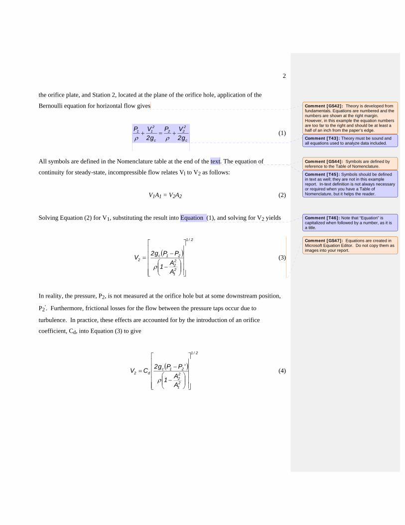
the orifice plate, and Station 2, located at the plane of the orifice hole, application of the

Bernoulli equation for horizontal flow gives

c

222

c

211

g2

VP

g2

VP

(1)

All symbols are defined in the Nomenclature table at the end of the text. The equation of

continuity for steady-state, incompressible flow relates Vl to V2 as follows:

V1A1 = V2A2 (2)

Solving Equation (2) for V1, substituting the result into Equation (1), and solving for V2 yields

2/1

21

22

21c2

AA

1

PPg2V

(3)

In reality, the pressure, P2, is not measured at the orifice hole but at some downstream position,

P2'. Furthermore, frictional losses for the flow between the pressure taps occur due to

turbulence. In practice, these effects are accounted for by the introduction of an orifice

coefficient, Cd, into Equation (3) to give

2/1

21

22

21cd2

AA

1

'PPg2CV

(4)

Comment [GS42]: Theory is developed from fundamentals. Equations are numbered and the numbers are shown at the right margin. However, in this example the equation numbers are too far to the right and should be at least a half of an inch from the paper’s edge.

Comment [T43]: Theory must be sound and all equations used to analyze data included.

Comment [GS44]: Symbols are defined by reference to the Table of Nomenclature.

Comment [T45]: Symbols should be defined in text as well; they are not in this example report. In-text definition is not always necessary or required when you have a Table of Nomenclature, but it helps the reader.

Comment [T46]: Note that “Equation” is capitalized when followed by a number, as it is a title.

Comment [GS47]: Equations are created in Microsoft Equation Editor. Do not copy them as images into your report.

3

Figure 1 Sharp-edged orifice meter with corner taps, copied from Crane (1957).

Finally, it is common to incorporate the area-ratio factor into a modified orifice coefficient, C,

defined as

1/ 22221

1

dCC

AA

(5)

Equation (4) is then simplified to

Comment [GS48]: This figure was prepared by scanning the original.

Comment [T49]: The figure here is a bit too large for the purpose. Efficient use of space should be considered, as some reports and papers may have a page limit. However, when you do shrink existing figures or create new figures, be sure to avoid compression artifacts and fonts that are too small to read. You should not go below 9pt for your smallest text in a figure, and some audiences will require even larger fonts. To remove compression artifacts, save images in higher resolutions before they are imported into your document. Most journals will not accept figures with a resolution less than 300 dpi (dots per inch) and often require much more. In this class and to keep file size down, screen resolution will be sufficient for figures (at 100% magnification, compression artifacts should not be obvious). Also, keep image file format in mind. For example, gif images are best for plots, line drawings, and text, but jpg images may be best for photographs.

Comment [T50]: As is done here, make sure you reference figures you did not create. It is also good practice to explicitly state in the caption that the figure was copied or adapted from another author. Although and again, this is not an appropriate way to reference. Also note that the title and caption are at the bottom of the figure, as they should be. However, the figure title in the Table of Figures is different than the one shown here, which could potentially confuse the reader. A better, and consistent caption would be: “Figure 1: Orifice Meter. Sharp-edged orifice meter with corner taps, copied from Crane [2].”

4

1/ 2

1

2g PV C

(6)

where (-P) = P1 - P2'.

More conveniently, Equation (6) may be written in terms of the mass-flow rate where

22AVm (7)

Substitution of Equation (7) into Equation (6) produces

2/1c2 Pg2CAm (8)

Alternatively, for an incompressible fluid, a volumetric-flow form of Equation (8) can be

derived. Since

Q = V2A2 (9)

Equation (6) may be written as

(10)

Equation (10) was used to compute the orifice coefficient C from experimental data.

As discussed in detail by the ASME Research Committee on Fluid Meters (1971), the orifice

coefficient, C, depends mainly on the type of orifice hole, the area ratio, A2/A1, the location of

the pressure taps, and the pipe Reynolds number given by

Q CA 2

2gc (P)

1/ 2Comment [GS51]: We finally arrive at the working equation.

5

(11)

Alternatively, the Reynolds number can be written in terms of the volumetric flow rate as

(12)

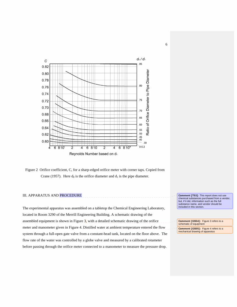
In this study, a square-edged orifice meter with corner taps was used. This type of orifice meter

is mentioned but not discussed in detail in the ASME (1971) work. It is considered in NACA

TM 952 (1940), which presents the orifice coefficient correlation redrawn in Crane T.P. 410

(1957) and shown in Figure 2. As would be expected from friction considerations, the orifice

coefficient is seen to decrease with decreasing ratio of orifice diameter to pipe diameter.

However, in no case is the orifice coefficient less than 0.59. Above a pipe Reynolds number of

200,000, depending on the ratio D2/D1, the orifice coefficient is independent of Reynolds

number. The experimentally derived values of C from this study were compared with the

correlation of Figure 2.

It should be noted that the use of the orifice discharge coefficient, Cd, is more common than the

use of the orifice coefficient, C, because the value of Cd asymptotically approaches a constant

value of approximately 0.61 at high values of the pipe Reynolds numbers. The orifice

coefficient, C, was used in this study so as to be consistent with the literature correlation of

Fig.2.

N Re1

D1V1

N Re1

4QD1

Comment [GS52]: Comparison with correlation from the literature.

6

Figure 2 Orifice coefficient, C, for a sharp-edged orifice meter with corner taps. Copied from

Crane (1957). Here d0 is the orifice diameter and d1 is the pipe diameter.

III. APPARATUS AND PROCEDURE

The experimental apparatus was assembled on a tabletop the Chemical Engineering Laboratory,

located in Room 3290 of the Merrill Engineering Building. A schematic drawing of the

assembled equipment is shown in Figure 3, with a detailed schematic drawing of the orifice

meter and manometer given in Figure 4. Distilled water at ambient temperature entered the flow

system through a full-open gate valve from a constant-head tank, located on the floor above. The

flow rate of the water was controlled by a globe valve and measured by a calibrated rotameter

before passing through the orifice meter connected to a manometer to measure the pressure drop.

Comment [T53]: This report does not use chemical substances purchased from a vendor, but, if it did, information such as the full substance name, and vendor should be included in this section.

Comment [GS54]: Figure 3 refers to a schematic of equipment

Comment [GS55]: Figure 4 refers to a mechanical drawing of apparatus

7

The water was discharged to a floor drain. The flow system used one-inch Schedule 40 steel pipe

throughout and was designed to operate in a continuous, steady-state, steady-flow mode.

Detailed specifications and dimensions of the major items of equipment in the flow system are

listed in Table E-l in Appendix E. The rotameter was rated for a nominal full-scale flow capacity

of 20 gpm of water at 20°C. The manufacturer's calibration curve is included as Fig. C-l in

Appendix C and was not verified in this study. The diameter of the orifice as measured with

inside calipers and a micrometer was 0.299 inches, giving an orifice-diameter-to-inside-pipe

diameter ratio, Do/Dp, of 0.285.

The operating procedure included the following steps.

1. The constant-head water tank was checked to be sure it was functioning properly.

2. The manometer was checked for the absence of air bubbles in the water legs above the

mercury and for identical levels for Hl and H2.

3. The globe valve was closed.

4. The gate valve was fully opened.

5. The globe valve was slowly opened until a desire and steady reading on the rotameter was

observed.

6. The mercury levels in the manometer were observed. If oscillation was occurring, the

manometer valves were used to dampen the oscillations so as to obtain constant mercury

levels.

7. The following readings were taken:

a) Location of the bob float in the rotameter. The float was read at the location shown

by the arrow in Fig. D-l.

b) Location of the mercury-water interface levels on both sides of the manometer. The

tops of the meniscuses were read.

c) Temperature of the water in the constant-head tank using a mercury-in-glass

thermometer.

8. Steps 4 through 6 were repeated for a new rotameter setting.

Comment [T56]: The description of the experimental procedure should be detailed enough so that a chemical engineering student at another university could repeat the same experiments years later.

Comment [GS57]: Detailed specifications

Comment [GS58]: Operating procedure

Comment [T59]: Unless you are writing a SOP, it would be best to write this procedure in a more compact, paragraph form, instead of a numbered list. Furthermore, you only need enough information so that someone else can repeat your work. Opening the gate valve, for example, is a given.

8

Figure 3 Flow diagram of experimental system.

The density and viscosity of water over a small ambient-temperature range were required for

correlating the data. Based on data in Liley, Reid and Buck (1984), the density of water was

taken to be constant at 62.3 lb/ft3, and the viscosity of water was estimated by use of the chart on

page 3-252 of this reference.

Comment [GS60]: This is a flow diagram. It shows the functional relationships and flow directions for the important pieces of equipment. It is not intended to be a picture of the apparatus. A photograph can be included in addition to the flow diagram if it is needed. Flow diagrams are generally more informative than photographs.

Comment [T61]: Figures must be neat and informative. They should be created with computer software of your preference.

Comment [GS62]: Physical properties.

9

Figure 4 Schematic of orifice meter and manometer.

IV. RESULTS AND DISCUSSION OF RESULTS

The experimental raw data are listed in Table A-l of Appendix A. Six runs were made, each at a

different flow rate. As shown, the rotameter reading varied over a 3.6 fold range from 7.5

percent to a maximum of 28.5 percent of full scale, corresponding to a water flow rate range of

approximately 1.6 to 5.7 gpm. The water temperature varied from 17.5 to 22°C.

Comment [GS63]: This is a mechanical drawing that shows, more or less to scale, the physical relationships of the parts of the orifice meter-manometer system.

Comment [GS64]: Raw data.

10

The manometer readings H2 and H1, shown in Figure 4, were converted to pressure drop by the

following equation based on the principles of fluid statics:

cO2HHg12 g

gHHP (13)

The rotameter readings were converted to volumetric flow rates with the calibration curve given

in Appendix D. The orifice area, A2, was computed from the orifice diameter, D2, to be 0.0702

in2 or 0.000488 ft2. The orifice coefficient and accompanying Reynolds number were computed

for each run from Equations (10) and (12), respectively. Sample calculations are given in

Appendix B.

The calculated results for all six runs are listed in Table 1 and plotted in Figure 5, where it is

seen that the orifice coefficients varied in a random fashion from 0.572 to 0.631 for a 3.4-fold

pipe-Reynolds-number range of from almost 5,000 to more than 16,000. Included in Figure 5 is

a literature curve from the previously mentioned NACA (1940) report showing an almost

constant value of 0.60 for the orifice coefficient. In general, our experimental data straddle the

literature curve with data below the curve for pipe Reynolds numbers in the transition region

(2,100 < NRe, < 10,000) and data above the curve for turbulent-flow Reynolds numbers. In this

latter region, our average measured orifice coefficient is 0.623, which is almost 4 percent higher

than the literature value. In the transition region, our measured coefficients are from 3 to 5

percent lower than the literature values.

According to Sakiadis (1984), a new and clean square-edged orifice is considered to be accurate

to within 1 to 2 percent when used with published correlations for the orifice coefficient. Our

experimental data were not within that range of accuracy. There are several possible reasons for

lack of accuracy:

1. The use of a sharp-edged (conical-edge) orifice. According to ASME (1971), research on

square-edged orifices has shown that measured coefficients are subject to installation and

inlet conditions. This may be particularly true for the transition region of flow, where our

first two runs were made. The ASME does not recommend sharp-edged orifices.

Comment [T65]: Symbols should be in italics and identically formatted throughout the report. Note that in the equations in this example report the symbols are in italics and in the text they are not. Generally, it is best to use italics for symbols throughout; they make your symbols easy to spot in the text and match the formatting of most equation authoring software.

Comment [T66]: Specific equations from the Theory section are used and referenced in this section.

Comment [GS67]: Calculated results.

Comment [T68]: Data are reported and discussed.

Comment [GS69]: Accuracy.

11

Table 1

Calculated results.

Run Flow

Rate, Q,

ft3/s

Orifice

Temp.,

F

Orifice

(-P),

lbf/ft2

Orifice

Coefficient

Pipe

Reynolds

Number

1 0.00343 71.6 146 0.57 4,900

2 0.00571 70.7 391 0.58 8,000

3 0.00822 70.7 694 0.63 11,600

4 0.01050 68.0 1,124 0.63 14,200

5 0.01164 65.3 1460 0.61 15,000

6 0.01301 63.5 1790 0.62 16,300

Figure 5 Comparison of measured orifice coefficients to reported values. The indicated

uncertainties are at the 95 % confidence level and are summarized in Table E-1.

Literature curve (NACA TM 952)

0.4

0.45

0.5

0.55

0.6

0.65

0.7

4000 6000 8000 10000 12000 14000 16000 18000

Pipe Reynolds Number

Literature curve (NACA TM 952)

0.4

0.45

0.5

0.55

0.6

0.65

0.7

4000 6000 8000 10000 12000 14000 16000 18000

Pipe Reynolds Number

Comment [GS70]: A simple table presents the experimental findings in a compact form. More detailed tables appear in the appendices, as needed.

Comment [T71]: Note that the title should be at the top of the table, unlike figures.

Comment [T72]: Units are given.

Comment [GS73]: This figure was prepared in Excel and modified in PowerPoint.

Comment [T74]: Error bars are given and the method for their determination is described.

12

2. The use of corner taps. Although no reason is given, ASME (1971) omits any

recommendation or correlation for orifice meters with corner taps.

3. Lack of sufficient length of straight pipe upstream of the orifice plate, particularly for runs

where the pipe Reynolds number was in the transition region. For accuracy and

reproducibility, the flow should be fully developed before reaching the orifice. In our

apparatus, only 10 diameters of straight pipe were provided upstream of the orifice. ASME

(1971) recommends 13 diameters for our piping configuration.

4. Location of the globe valve used to control the flow rate of water. For the location shown in

Figure 3, the pressure drop across the valve could have caused a release of dissolved air in

the form of bubbles downstream of the valve. The presence of bubbles in the water flowing

through the rotameter could have caused an error in the flow rate measurement; however, the

presence of bubbles was not observed.

5. Uncertainties in measurements (95% confidence level). Assuming that the calibration curve

for the rotameter and the physical properties of the fluids were known with certainty, the

uncertainties, with a 95% confidence level, were estimated to be as follows:

a) Rotameter reading, ± 0.5 (for a scale of 0 to 100)

b) Manometer levels, ± 0.05 inch

c) Thermometer reading, + 0.25°C

d) Orifice diameter, + 0.001 inches.

In addition, based on information in Sakiadis (1984), it was assumed that the uncertainty in

the standard inside-pipe diameter of 1.049 inches was ± 0.02 inches.

The propagation of the above uncertainties into the equations used to process the data is

presented in detail in Appendix F. The resulting uncertainty in the calculated orifice coefficients

ranges from ± 0.07 at the lowest NRe1 down to ±0.01 at the highest NRe1. The corresponding

uncertainty in NRe1 ranges from ± 340 to ± 440. The uncertainty in , the ratio of orifice diameter

to pipe inside diameter, is ± 0.006.

Comment [GS75]: Uncertainties should always be given with the specified confidence level.

13

The uncertainties are depicted in Figure 5 by including horizontal and vertical extensions on the

six experimental data points. Figure 5 shows that, after the uncertainties are taken into account,

the experimental data are generally in agreement with the literature correlation.

V. CONCLUSIONS AND RECOMMENDATIONS

Orifice coefficients were determined experimentally for the flow of water at pipe Reynolds

numbers from approximately 5,000 to 16,000 through a sharp-edged, 0.299-inch diameter orifice

installed in a Schedule 40 one-inch steel pipe and provided with corner taps. The coefficients

varied irregularly with pipe Reynolds number from a low of 0.57 in the transition region to a

high of 0.63 under turbulent-flow conditions.

Compared to a literature correlation, our orifice coefficients are 3 to 5 percent lower at pipe

Reynolds numbers in the transition region below 10,000. For turbulent-flow Reynolds numbers,

our coefficients are 2 to 5 percent higher than the literature correlation. Thus, our values are not

within the 1 to 2 percent deviation range claimed by ASME (1971) for a well-designed orifice

meter. The discrepancies were explained by experimental uncertainties, based on our best

judgment of the uncertainty for each of our measurements.

An additional explanation for the deviation of our results is the unreliability of a square-edged

orifice with corner taps, particularly when it is operated in the transition region without a suitable

inlet length that will guarantee that fully developed flow occurs before the flow reaches the

orifice plate.

It is recommended that a carefully machined square-edged orifice plate, between flanges with

carefully machined flange taps, be installed, following the recommendations of the ASME

Research Committee on Fluid Meters (1971). Extensive studies show that this type of orifice

meter gives results that are reproducible to within 1 to 2 percent. Furthermore, it is recommended

that the location of the globe valve be changed from upstream to downstream of the rotameter

and that the inlet length of straight pipe just upstream of the orifice meter be increased to at least

13 pipe diameters.

Comment [GS76]: Conclusions.

Comment [T77]: Concisely recap. Restate the objectives, what was done, and the results.

Comment [GS78]: Recommendations.

14

NOMENCLATURE

Symbol Definition Units

A1 Inside cross sectional area for the pipe ft2

A2 Cross sectional area for the orifice hole ft2

C Orifice coefficient -

Cd Orifice discharge coefficient -

Dp Inside pipe diameter ft

Do Orifice hole diameter ft

g Acceleration due to gravity ft/s2

gc Universal constant, 32.2 lb-s2/lbf-ft

H1 Lower manometer-fluid level ft

H2 Higher manometer-fluid level ft

m. Mass flow rate lb/s

NRe1 Pipe Reynolds number -

P1 Pressure in pipe upstream of orifice lbf/ft2

P2 Pressure at plane of orifice hole lbf/ft2

P2' Pressure in pipe downstream of orifice lbf/ft2

Q Volumetric flow rate ft3/s

RR Rotameter reading % of full scale

T Temperature °C or °F

V1 Fluid velocity in pipe ft/s

V2 Fluid velocity in orifice hole ft/s

Greek

Ratio of orifice-hole diameter to pipe ID -

-P Pressure drop across the orifice, P1- P'2 lbf/ft2

i Uncertainty in measurement (depends on i)

Comment [GS79]: Every symbol that appears in the text must appear in this table and be defined. The dimension of each must be given. If a quantity is dimensionless, a hyphen is used to so indicate.

Comment [T80]: Symbols are listed alphabetically, with Greek letters in a separate section, to make it easier for the reader to find a symbol of interest.

15

Fluid density lb/ft3

Fluid viscosity lb/ft-s

16

REFERENCES

ASME, Fluid Meters: Their Theory and Application", Sixth Ed., Bean, H. S. Ed., ASME

Research Committee on Fluid Meters, New York, NY, p 58-60, 73, 179-208, 211-215, (1971)

Crane, "Flow of Fluids Through Valves and Fittings," Crane Technical Paper 410, Crane

Company, Chicago, Ill. p A19, (1957)

de Nevers, N., Fluid Mechanics, Addison-Wesley, Reading, MA , p 131, 139, and 144, (1970)

Liley, P.E., R.C. Reid and Evan Buck, "Physical and Chemical Data", in Perry's Chemical

Engineers' Handbook, Sixth Ed., D. Green and J. O. Maloney, Eds., McGraw-Hill, New York,

NY, p 3-75, ( 1984)

NACA, "Standards for Discharge Measurement With Standardized Nozzles and Orifices", NACA

Technical Memorandum 952, NASA, Washington, D.C., p 4, 24; Data sheet 1; Figure IV, (Sept.

1940).

Sakiadis, B.C., "Fluid and Particle Mechanics", in Perry's, op cit." p 3-251, 5-14 to 5-16 and 6-

42. (1984).

Silcox, G. D., "Basic Analysis of Data," unpublished printed notes, Univ. of Utah, Salt Lake

City, Utah (1999).

Comment [GS81]: Every document referred to in the text is listed in the References. The style chosen here lists them alphabetically. While this method is acceptable in some publications, for this course, you should list references in a numbered list by order of their appearance in the text. Therefore these references should be reordered and numbered: For example: 1. de Nevers, N., Fluid Mechanics, Addison-Wesley, Reading, MA , p 131, 139, and 144, (1970) 2. Sakiadis, B.C., "Fluid and Particle Mechanics", in Perry's, op cit." p 3-251, 5-14 to 5-16 and 6-42. (1984). 3. ASME, Fluid Meters: Their Theory and Application", Sixth Ed., Bean, H. S. Ed., ASME Research Committee on Fluid Meters, New York, NY, p 58-60, 73, 179-208, 211-215, (1971) And so on…

17

APPENDICES

APPENDIX A

RAW DATA

Table A-l

Raw experimental data obtained October 16, 1985.

Run Rotameter

Reading, % Full

Scale

Manometer

Height, H2,

inches

Manometer

Height, H1,

inches

Water

Temp., °C

1 7.5 1.30 -0.95 22.0

2 12.5 3.20 -2.80 21.5

3 18.0 5.55 -5.10 21.5

4 23.0 8.85 -8.40 20.0

5 25.5 11.40 -11.00 18.5

6 28.5 13.95 -13.50 17.5

Comment [T82]: The data collected. If you have extensive amounts of raw data, it may be more appropriate to hand in a CD or DVD with your report. Note that units are always given. There should be some indication of uncertainty.

18

APPENDIX B

SAMPLE CALCULATIONS

The following sample calculations use the raw data from Run 1 of Table A-l in Appendix A.

Constants

Hg = (13.55)(62.3) = 844.2 lb/ft3

H20 = 62.3 lb/ft3

g = 32.2 ft/s2

gc = 32.2 lb-s2/lbf-ft

D1 = inside pipe diameter = 1.049 in = 0.0874 ft

D2 = orifice diameter = 0.299 in = 0.0249 ft

A2 = orifice cross sectional area = 0.0702 in2 = 0.000488 ft2

= D2/Dl = 0.285

Run data

Rotameter reading = 7.5 % of full scale

H2 = 1.30 in = 0.108 ft

H1 = - 0.95 in = -0.079 ft

T = 22.0°C = 71.6°F

Calculation of Flow Rate

From Appendix C, the correlating equation for the manufacturer's rotameter calibration is

RR = 0.0775 Q (B-l)

where RR = rotameter reading, % of full scale, Q is the Volumetric flow rate of water at 20°C in

cm3/s. If the effects of water temperatures in the range of 17.5 to 22°C are neglected, the

rotameter calibration equation for flow rates in ft3/s becomes

Comment [GS83]: Detailed sample calculations with all data sources.

Comment [GS84]: Explanation of how the calculation is made. This should be similar in style and detail to what appears in most textbooks.

19

(B-2)

where Q is in ft3/s. Then

Calculation of (-P)

From Equation (13),

2

cO2HHg12

ft/lbf146

2.32

2.323.622.844079.0108.0

g

gHHP

Calculation of Orifice Coefficient

From Equation (10),

and

2/1

c1

Pg2A

QC

(B -3)

572.0

3.621462.322

000488.0

00343.02/1

Q

RR

2190

Q

7.5

2190 0.00343

ft

s

Q CA 2

2gc (P)

1/ 2

20

Calculation of the Pipe Reynolds Number

We used linear interpolation for the water-viscosity data in the section “Apparatus and

Procedure."

Viscosity of water at 71.6°F =

From Equation (12)

The above-calculated results for Run 1 are listed in Table 1.

0.978 (0.978 0.953)71.6 70

72 70

0.958 cp 0.000644lb

ft s

N Re1

4QD1

(4)(0.00343)(62.3)

(3.14)(0.0874)(0.000644)

4840

21

APPENDIX C

ROTAMETER CALIBRATION

Figure C-1 Rotameter calibration curve, copied from the report of JWS.

Comment [T85]: This section should contain enough information that the reader may judge the precision of your calibrated equipment. In this example, a linear fit seems to be adequate, but some indication of the goodness of fit should be given.

Comment [GS86]: Note that the author is using a calibration prepared by JWS (a student from the previous year) without giving a reference in the Reference Section. This is unacceptable.

22

APPENDIX D

MAJOR ITEMS OF EQUIPMENT

Table D-l

Specifications and dimensions of major items of equipment.

1. Rotameter:

Fisher and Porter Company, Model l0A3665A with FP-1-60-P-8 tube guide and NSVP-622 bob

float. Manufacturer's calibration curve is given in Fig. C-l of Appendix C.

2. Orifice Meter and Piping:

Sharp-edged orifice with corner taps located in one-inch Schedule 40 steel pipe.

Measured orifice diameter = D2 = 0.299 in.

Inside pipe diameter D1 = 1.049 in.

(from page 6-42 of Sakiadis (1984)).

D2/D1 = 0.285

Length of orifice cylindrical section: 0.02 inches

Angle of chamfer: 45°

Length of pipe between ell and orifice plate: 10.5 inches.

3. Manometer:

Dwyer model 36-W/M glass, U-tube manometer, with valves to dampen oscillation, and using

mercury (s.g. = 13.55) as the manometer fluid.

Comment [T87]: Sufficient detail is given so that another researcher could obtain the equipment and repeat the same experiments. If chemicals were used in this project, they would be listed here with their manufacturing information (manufacturer, purity, lot number…).

23

APPENDIX E

UNCERTAINTY ANALYSIS

The following uncertainties (95% confidence level) were estimated for the experimental

measurements:

RR = ± 0.5

H1 =H2 = 0.05 in. = 0.00417 ft

T = ± 0.25°C

D1 = ± 0.02 in. = ± 0.00167 ft

D2 = ± 0.001 in. = ± 0.0000833 ft

Uncertainty in the Orifice Coefficient:

Combining Equations B-2, 13, and B-3 with the relation, A2 = D22/4, gives

5.0

O2H

O2HHg1222

g))(HH(2

4D

2190

RRC

(E-1)

or

5.012

22 )HH(D48900

RRC

(E-2)

The uncertainties were propagated using a spreadsheet and the procedure discussed by Silcox

(1999). The results are summarized in Table E-1.

Comment [GS88]: The uncertainty analysis has no meaning unless the confidence level is specified.

Comment [T89]: The uncertainties in all physical measurements are given.

Comment [T90]: This example report should contain more information on how these uncertainties were calculated. A copy of the Excel worksheet may be an appropriate addition. Also, discussion of the sensitivity factors should be included in this section, so that the reader may understand how best to improve the experiments.

24

Uncertainty in the Pipe Reynolds Number

Combining Equations B-2 and 12, and using a polynomial to represent the viscosity of water as a

function of temperature, give the Reynolds number:

)10x201.1T*10x371.3T*10x664.3(D61.27

RRN

35271

Re (E-3)

The uncertainties were propagated using a spreadsheet and the procedure discussed by Silcox

(1999). The results are summarized in Table E-1.

Uncertainty in D2/D1 ratio

The ratio of diameters is

1

2

D

D (E-4)

The uncertainties were propagated using a spreadsheet and the procedure discussed by Silcox

(1999). The results are summarized in Table E-1.

Summary of Estimates in Uncertainty for All Six Runs

The estimated uncertainties are given in Table E-1. These uncertainties were incorporated in

Figure 5.

25

Table E-1

Uncertainties in calculated results (95% confidence level).

Run C NRe1

1 ±0.07 ±340

2 ±0.04 ±360

3 ±0.03 ±400

4 ±0.02 ±420

5 ±0.02 ±430

6 ±0.01 ±440

= ±0.006