Example 13.2Quarterly Sales of Johnson & Johnson

Regression-Based Trend Models

13.1 | 13.1a | 13.3 | 13.4 | 13.5 | 13.6 | 13.6a | 13.6b | 13.7 | 13.7a | 13.7b

Objective

To fit a linear trend line to Johnson & Johnson’s quarterly sales and examine its residuals for randomness.

13.1 | 13.1a | 13.3 | 13.4 | 13.5 | 13.6 | 13.6a | 13.6b | 13.7 | 13.7a | 13.7b

JOHNSON&JOHNSON.XLS

This file contains quarterly sales data for Johnson & Johnson from second quarter 1991 through first quarter 2001.

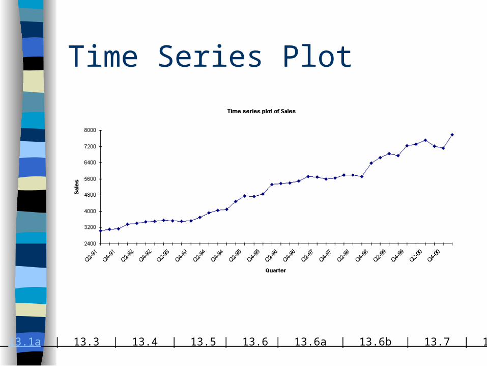
The time series plot of these data appears on the next slide.

Sales increase from $3031 million in the initial quarter to $7791 million in the final quarter.

How well does a linear trend fit these data? Are the residuals from this fit random?

13.1 | 13.1a | 13.3 | 13.4 | 13.5 | 13.6 | 13.6a | 13.6b | 13.7 | 13.7a | 13.7b

Time Series Plot

13.1 | 13.1a | 13.3 | 13.4 | 13.5 | 13.6 | 13.6a | 13.6b | 13.7 | 13.7a | 13.7b

Linear Trend

A linear trend means that the time series variable changes by a constant amount each time period.

The relevant equation is Yt = a + bt + Et where a is the intercept, b is the slope and Et is an error term.

If b is positive the trend is upward, if b is negative then the trend is downward.

The graph of the time series is a good place to start. It indicates whether a linear trend model is likely to provide a good fit.

13.1 | 13.1a | 13.3 | 13.4 | 13.5 | 13.6 | 13.6a | 13.6b | 13.7 | 13.7a | 13.7b

Solution The plot indicates a clear upward trend with little or

no curvature.

Therefore, a linear trend is certainly plausible.

To estimate it with regression, we first need a numeric time variable – labels such as Q2-91 will not do.

We construct this time variable in column C of the data set, using consecutive values 1 through 40. This is shown in the table on the next slide.

13.1 | 13.1a | 13.3 | 13.4 | 13.5 | 13.6 | 13.6a | 13.6b | 13.7 | 13.7a | 13.7b

Regression Output for Linear Trend

13.1 | 13.1a | 13.3 | 13.4 | 13.5 | 13.6 | 13.6a | 13.6b | 13.7 | 13.7a | 13.7b

Solution -- continued We then run a simple regression of Sales versus Times,

with the results shown.

The estimated linear trend line isForecasted Sales = 2585 +122.77Time

This equation implies tat we expect sales to increase by $122.77 million per quarter.

To use this equation to forecast future sales, we start with the final sales figure, 7791 in Q1 of 2001, and add 122.77 times the number of quarters in the future being forecasted.

13.1 | 13.1a | 13.3 | 13.4 | 13.5 | 13.6 | 13.6a | 13.6b | 13.7 | 13.7a | 13.7b

Solution -- continued Excel supplies an easier way to obtain this trend line.

Once the plot is constructed, we can use the Chart/Add Trendline menu item. This gives us several types of trend lines to choose from, and we select the linear option for this example.

We can also click on the Options tab in the Add Trendline dialog box and select the options to show the regression equation and its R2 value on the chart, as we have done on the plot on the next slide. This superimposed trend line indicates a reasonably good fit.

13.1 | 13.1a | 13.3 | 13.4 | 13.5 | 13.6 | 13.6a | 13.6b | 13.7 | 13.7a | 13.7b

Time Series Plot with Linear Trend Superimposed

13.1 | 13.1a | 13.3 | 13.4 | 13.5 | 13.6 | 13.6a | 13.6b | 13.7 | 13.7a | 13.7b

Solution -- continued However, the fit is not perfect, as the plot of the residuals

shows on the next slide.

These residuals tend to “meander,” staying positive for a while, then negative, then positive, and so on.

You can check that the runs test for these residuals produces a z-value of –3.204, with a corresponding p-value of 0.001.

In short, these residuals are not random noise, and they could be modeled further. However, we do not have the tools to do so in this book.

13.1 | 13.1a | 13.3 | 13.4 | 13.5 | 13.6 | 13.6a | 13.6b | 13.7 | 13.7a | 13.7b

Time Series Plot of Residuals