examination of residuals - project...
TRANSCRIPT

EXAMINATION OF RESIDUALSF. J. ANSCOMBE
PRINCETON UNIVERSITY AND THE UNIVERSITY OF CHICAGO
1. Introduction
1.1. Suppose that n given observations, yi, Y2, * , y., are claimed to be inde-pendent determinations, having equal weight, of means pA, A2, * *X, n, such that(1) Ai= E ai,Or,
where A = (air) is a matrix of given coefficients and (Or) is a vector of unknownparameters. In this paper the suffix i (and later the suffixes j, k, 1) will alwaysrun over the values 1, 2, * , n, and the suffix r will run from 1 up to the num-ber of parameters (t1r).
Let (#r) denote estimates of (Or) obtained by the method of least squares,let (Yi) denote the fitted values,
(2) Y= Eai,
and let (zt) denote the residuals,(3) Zi =Yi - Yi.If A stands for the linear space spanned by (ail), (a,2), *-- , that is, by thecolumns of A, and if X is the complement of A, consisting of all n-componentvectors orthogonal to A, then (Yi) is the projection of (yt) on A and (zi) is theprojection of (yi) on Z. Let Q = (qij) be the idempotent positive-semidefinitesymmetric matrix taking (y1) into (zi), that is,
(4) Zi= qtj,yj.
If A has dimension n - v (where v > 0), X is of dimension v and Q has rank v.Given A, we can choose a parameter set (0,), where r = 1, 2, * , n -v, suchthat the columns of A are linearly independent, and then if V-1 = A'A andif I stands for the n X n identity matrix (6ti), we have
(5) Q =I-AVA'.The trace of Q is
(6) qii = v.
Research carried out at Princeton University and in part at the Department of Statistics,University of Chicago, under sponsorship of the Logistics and Mathematical Statistics Branch,Office of Naval Research.

2 FOURTH BERKELEY SYMPOSIUM: ANSCOMBE
The least-squares method of estimating the parameters (Or) is unquestionablysatisfactory under the following
Ideal statistical conditions. The (yi) are realizations of independent chance vari-ables, such that the (yi- js,) have a common normal distribution with zero mean.That is to say, given the ideal conditions, the least-squares estimates of the
parameters, together with the residual sum of squares, constitute a set of suf-ficient statistics, and all statements or decisions resulting from the analysis willproperly depend on them. They may also depend on a prior probability or losssystem, and estimates eventually quoted may therefore differ from the least-squares estimates, as C. M. Stein has shown.We shall refer to the differences (yi-,i') by the conventional name of "er-
rors," and denote the variance of the error distribution by o.2. Under the idealconditions, QO2 is the variance matrix of the residuals (zi), which have a multi-variate normal chance distribution over N. We shall denote by 82 the residualmean square, (1z2)/v, which under the ideal conditions is an unbiased estimateof a2.
1.2. The object of this paper is to present some methods of examining theobserved residuals (z;), in order to obtain information on how close the idealconditions come to being satisfied. We shall first (section 2) consider the residualsin aggregate, that is, their empirical distribution, and then (section 3) considerthe dependence of the residuals on the fitted values, that is, the regression rela-tions of the pairs (Yi, zi). In each connection we shall propose two statistics,which can be taken as measures of departure from the ideal conditions and canbe used as criteria for conventional-type significance tests, the ideal conditionsbeing regarded as a composite null hypothesis. Section 4 will be concerned withjustifying the statistics proposed, and section 5 with examples of their use.The problem of examining how closely the ideal conditions are satisfied is very
broad. Despite the immense use of the least-squares methods for well over acentury, the problem has received no comprehensive treatment. Particular as-pects have been considered by many authors, usually on a practical rather thantheoretical level. This paper, too, is concerned with particular aspects, except fora little general discussion in section 6. The reader will appreciate that it is notalways appropriate to base an investigation of departures from the ideal condi-tions on an examination of residuals. This will be illustrated below (section 5.5).And if residuals are examined, many other types of examination are possiblebesides those presented here. For example, when the observations have beenmade serially in time, and time is not among the parameters (Or), interestinginformation may possibly be obtained by plotting the residuals against time, asTerry [17] has pointed out. There are circumstances in which the error variancemay be expected to be different for different levels of some factor, as for exam-ple in a plant-breeding experiment when the lines compared differ markedly ingenetic purity. The ways in which the ideal conditions can fail to obtain are ofcourse countless.The material of this paper has been developed from7two sources: first, some
EXAMINATION OF RESIDUALS 3
unpublished work relating primarily to the analysis of data in a row-columncross-classification, done jointly with John W. Tukey [1], [4]-to him is duethe idea of considering simple functions of the residuals, of the type here pre-sented, as test criteria; second, a study of correlations between residuals, inconnection with an investigation of rejection rules for outliers [3]. Familiaritywith the latter is not assumed, but overlap has been kept to a minimum, withthe thought that a reader interested in this paper will read [3] also.
1.3. The methods developed below appear not to have any sweeping optimumproperties. They are easiest to apply, and possibly more particularly appropri-ate, if the following two conditions are satisfied.
Design condition 1. A contains the unit vector, or (in other words) the param-eter set (Or) can be so chosen that one parameter is a general mean and the correspond-ing column of A consists entirely of 1's.
Design condition 2. The diagonal elements of Q are all equal, thus qji = v/n(for all i).
These are labeled "design conditions" because they are conditions on A. If theobservations come from a factorial experiment, A depends on the design of theexperiment, in the usual sense, and also on the choice of effects (interactions,and so forth) to be estimated, so the name is not entirely happy, but will beused nevertheless.
Condition 1 is, one supposes, almost always satisfied in practice. If it were not,and if the residuals were to be examined, the first idea that would occur wouldbe to examine the mean of the residuals, and that would be equivalent to intro-ducing the general mean as an extra parameter, after which condition 1 wouldbe satisfied. So this condition is not much of a restriction. A consequence of thecondition is that every row (or column) of Q sums to zero, that is, E qi; = 0 foreach i. Hence if p denotes the average correlation coefficient between all pairs(zi, z,), where i Fd j, we have
(7) 1 + (n -l)p = O.
The residuals themselves sum to zero, and so their average z = 0.Condition 2 is satisfied for a broad class of factorial and other randomized
experimental designs, provided that the effects estimated do not depend for theirdefinition on any quantitative relation between the levels of the factors. Inother circumstances we shall expect condition 2 not to be satisfied exactly. Aconsequence of condition 2 and the idempotency of Q is that the sum of squaresof entries in any row (or column) of Q is the same, namely
(8) E (qij)2 = qii -nVnHence if p2 is the average squared correlation coefficient between all pairs (zi, zi),where i $P j, we have
(9) 1 + (n-l)p2 = vii

4 FOURTH BERKELEY SYMPOSIUM: ANSCOMBE
Condition 2 was imposed in the study of outliers [3], in order to avoid any ques-tion as to the correct weighting of the residuals. Ferguson [10] has consideredoutliers when condition 2 is not satisfied.
In the next two sections we shall proceed first without reference to conditions1 and 2, and then we shall see how the expressions obtained reduce when condi-tions 1 and 2 are introduced.
2. Empirical distribution of residuals
2.1. Skewness. Let us suppose-that--theideal statistical conditions obtain, asin the above enunciation, wxcet that we delete the word "normal." Let yiand Y2 be the first two scale-invariant shapehce ste) of theerror distribution, measuring skewness and kurtosis, defined as
(10) ' =I E[(yi - Ai)3], Y2 = -4 IE[(yi- Ai)4] - 3a'}.
We shall study estimates g1 and 92 of ay and 72, based on the statistics s2, ,iz3_iz4, analogous to Fisher's statistics [13] for a simple homogeneous sample.Since we suppose the errors (yi -ui) to be independent with zero means, we
have at once(11) E(E z3) = E_ (qij)3,y1a3.
t ij
Provided _ij(qii)3 i 0, we can define gi by3zi
(12) E (qxi)3s3ij
We now consider the sampling distribution of g1 under the full ideal condi-tions, so that yi = 0. The distribution of (zi) has spherical symmetry in X, andthe radius vector s is independent of the direction. Hence gi, being a homogeneousfunction of (zi) of degree zero, is independent of s, and we have
E[(F Z3)2](13) E(gl) = 0, Var (g1) =
ii
It is well known that E(s6) = (v + 2)(v + 4)a6/v2. As for the numerator, wehave E[(F_z3)2] = F_iE(z'z.J). Now, whether i and j are the same or different, z;and z; have a joint normal distribution with variance matrix
(14) o.2 (qii qij)qii qjj
It follows that E(Atz3j) is the coefficient of t'ti/(3!)2 in the expansion of themoment-generating function exp [(l/2)o-2(qiit21 + 2q,jtlt2 + q 2t2)]. We obtaineasily

EXAMINATION OF RESIDUALS 5
(15) E(z3z) = {6(qij)3 + 9qijqiiqjj} af.Hence
[6 E, (qj,)3 + 9 E qijqiiqjj]v2(16) Var (gi) = ji
[E (qij)3]2(P + 2)(v + 4)ii
Because Q is positive-semidefinite, the expression _ijqijqiiqjj is nonnegative.It vanishes under design conditions 1 and 2, or (more generally) if the vector(qii) lies in A. Then (16) reduces to
6v2(17) Var (Ui) = (v + 2)(v + 4) E (qij)3
ii
If p3 denotes the average cubed correlation coefficient between pairs (zi, zj),where i F6 j, (17) can be expressed under condition 2 as
6n2(18) Var (gi) =(18) ~~~v(v +2)(v +4){1 + (n -l)p3}
Under condition 2 g9 itself can be expressed as
n2 EZ3(19) 9 {1 + (n-2)32
For the simple homogeneous sample, v = n - 1 and p3 -1/iV3, and (18)reduces to Fisher's result,
(20) Var (g1) - 6n(n - 1)(n-2)(n + 1)(n + 3)
For a row-column cross-classification with k rows and 1 columns, n = kl andv = (k - 1)(1 - 1), and we find
(21) 1 + (n-1)p3 n(k -2)(1 -2).
Hence (18) gives, provided k and 1 both exceed 2,
(22) Var (g1) =6n(v + 2)(v + 4)(k-2)(1-2)
If n and v are both large, it is commonly (but not invariably) the case that1 + (n - 1)p is very close to 1, and then the right side of (18) is roughly6n2/v3, about the same as the variance of g9 for a homogeneous sample of sizev(v/n)2.
In principle it is possible by the same method to find higher moments of thesampling distribution of g1, under the full ideal conditions. It is easy to see thatthe odd moments vanish. The fourth moment is as follows.

6 FOURT'H BERKELEY SYMPOSIUM: ANSCOMBE
(23) E(gfi) =108yv (qij)3]2(v + 2)(v + 4)(v + 6)(v + 8)(v + 10)[, (qij)3]4 {[.ijij
+ 18 E (qij)2(qkz)2qikqjI + 12 E qijqikqilqjkcjlqklijkl iij/d
+ 36 Ei qijQjkqjl(qkl)2qii + 18 E qikqjl(qk ) 9i.Qjjijkd ijid
+ 6 E qilqjlqklqiiqjjqkk + 3 E qijqiiqjj E(1kl)ijkl ij kl
+9 (E qi,iiqjj)2q)4ij
Under conditions 1 and 2 the last five of the eight terms inside the braces vanish,leaving only the first three. Unfortunately the second and third terms are for-midable to evaluate, in general. By way of considering a relatively simplespecial case, let us impose the further design condition that all the off-diagonalelements of Q are equal, barring sign. (Such designs are illustrated below insection 5.4; they include the simple homogeneous sample.) Then if we write cfor v/n, the elements in every row of Q consist of c in the diagonal andi[c(l - c)/(n -1)]1/2 everywhere else, the number of minus signs exceedingthe number of plus signs (in these off-diagonal elements) by [c(n - 1)/(1-c)]1/2-which must of course be an integer. Writing C for c2 - c(I - c)/(n - 1), wefind easily that
(24) E (q,1)3 = vC,ij
and because _I(q,k)2qjl = Cqjk we have also
(25) (qjj)2(qkl)2qikqjl = C E (qij)3 = vC2.
I have been unable to evaluate completely the third term, 2ijklqijqikqilqjkqjlqkz,except for the simple sample, having v = n - 1 and C = (n - 2)/n, when itcan easily be shown to be (n - 1) (n - 2) (n - 3)/n2. On substitution into (23)we then verify Fisher's formula for E(gt) ([12], p. 22). For other designs havingequal-magnitude correlations, we can say that
(26) E qi,qikqilqjkqjlqkl = PC 4vc4(1 - c)ijkd n-i
+ 3vc3(1- C)2 _ 6v(n -2)c3(1 -c)2 + R,-~~~~ ~ ~n-1 (n -1)2
where the successive terms on the right side are the contributions to the totalsum from sets of suffixes (i, j, k, 1) that are (respectively) all equal, all but oneequal, equal in two different pairs, different except for one pair, and finallyR stands for the balance from sets of wholly unequal suffixes. R consists ofthe sum of n(n - 1)(n - 2)(n - 3) terms each equal to i[c(l - c)/(n - 1)]3.Now if n is large and c not very close to 0 or 1, positive and negative values areroughly equally frequent among the elements of Q, and it seems highly plausible

EXAMINATION OF RESIDUALS 7
that the terms of R almost cancel each other, so that R = o(n). Assuming this,we find, for n large and c constant,
(27) E(gt) ci91.{1 _(1c)}, E(g2)6 {1 -
Hence the kurtosis coefficient of the distribution of g1 is asymptotically 36/n,the same as for the simple sample of size n. Thus although the variance of giexceeds that for a simple sample of the same size n by a factor of (n/v)3 roughly,the shape of the distribution is apparently roughly the same. It is tempting tosurmise that the similarity of shape may hold true fairly generally for complexdesigns such that all the off-diagonal elements of Q are small.
2.2. Kurtosis. Consider now the estimation of the kurtosis coefficient 'Y2 ofthe error distribution, as posed at the outset of section 2. We find easily(28) E(_ zi) = E (q,)4o2a4 + 3 E (qii)2o4,
i ij i
(29) A2E(s4) = E[(FZ_)2] = E (qii)2 Y24 + v(v + 2)af.* t
We can therefore define g2 by the following expression, provided the divisor Ddoes not vanish,
(30) 92 = D-1,-i+2 D'where
3[E (qi.)2]2(31) D = (q,)4- v
ij pv(v+ 2)Under the full ideal statistical conditions, we have E(g2) = 0 and
(3v_E (qjj)2 \2 ZE[(Z4) 2](32) D2 Var (g2) + 1 v+2 ) E(s8)Proceeding as before we find
(33)E[( z4)2] = E(z4z) = {24 E (qi,)I + 72 E (qj,)2qjjqjj + 9[X (qij)2]2}o8
t ii ii ii t
and hence(34) ~~~~~~~(24D+ 72F)v,'(34) Var (g2) = D2(V + 2)(v + 4)(v + 6)
where
(35) F = E (qi,)2qiiqj,- v-'[ (qi)2]2.ii i
Under condition 2, F vanishes and we have
(36) 92 = s _ A%+ -_1,v(v + 2) fl + (n - lPpI- 3n v EZ,)2 n

8 FOURTH BERKELEY SYMPOSIUM: ANSCOMBE
(37) Var (92) =24n'[v(v + 2){1 + (n - 1);} - 3n](v + 4)(v + 6)
For the simple sample we obtain Fisher's result,
(38) Var (92) =24n(n-1)2(n-3)(n - 2)(n + 3)(n + 5)For the cross-classification with k rows and 1 columns we have
(39) Var (92) = ~~~~24n2p2[(v + 2)(k2 - 3k + 3)(12 - 31 + 3) - 3p2](p + 4)(v + 6)
If n and v are both large and 1 + (n - 1)p is close to 1, the right side of (37)is roughly 24n3/v4, about the same as the variance of g2 for a simple sample ofsize v(v/n)3.
It is possible to write down a general expression for E(g23), under the ideal con-ditions. We quote here only the reduced form under condition 2.
1728v {,E(q.,)2(q(k)2(qk)2 - 34(p + 8) - 6v D}(40) E(g2) =jk (n(v + 2)2 + 2)
(v + 2)(v + 4)(v + 6)(v + 8)(v + 10)D3For a design with equal-magnitude correlations, we find easily
E (qi.)2(qik)2(qik)2 = nC6 + 3nc4(1-c2+ n(n--2)c3(1-c)3cijk ~~~~~n-1n-)
(41) nc2(1 - c)2 3vc2D =nc4+ n -i
When n is large, that is, as n -x 00, with c > a positive bound, these give
(42) E(g2) -1728 Var (92) , 24
and the skewness coefficient of the distribution of 92 is asymptotically 6(6/n) 1/2the same as for a simple sample of size n.
3. Relation of residuals with fitted values
3.1. Heteroscedasticity. Let us suppose that a weakened form of the idealstatistical conditions obtains, namely: the (yi) are realizations of independentchance variables, such that y, - Ai has a1n_rmal distribution with zero mean andvariance proportional to exp (x,u,), where x is a constant. Denoting the varianceof yi by a2, we suppose that at oc exp (XMi), so that E(y; - Ai)2 has a regressionon Ai. If x is small, the regression is nearly linear. We shall study an estimate hof x, for x assumed small, based on the statistics 82 and tyz!Yi, that is, on an
empirical linear regression of (z2) on (Yi).Let F = v-lFiqiiYi, and let (r12) be the matrix taking (y,) into (Y,- 7),
that is,

EXAMINATION OF RESIDUALS 9
(43) Y - Y = ri,j, rij = bij - qij - V (qjj - E QjkQkk)-k
It is easy to show that Firijqjk = 0 for all i and k. Under the assumed conditions,z and Yfo(for any i) have a bivariate normal distribution, and(44)
E(zi) = 0, E[z1(Y - r)] = E qijrjj, Var (Yi- F) = E (rji)20,.Now suppose that x is small, so that(45) q2 = o2[1 + X(L, -u) + O(x2)],where p = v-1_iqjjjj. Then(46) E[zj(Y - _)]= qijrjj(,4j - )x2 + O(x2).
Thus (except in the degenerate case when rij = 0 for all j) the regression co-efficient of zi on Y,- is O(x). Hence the (quadratic) regression coefficientof Z2 on y- F is O(x2), that is,(47) E(zZ2 Y,- F) = E(z2) + O(x2).It follows that(48) E[E zt(Y - E)]= E(z)E(Yi-F) + O(X2)
= E (qij)2a2.(A j- ) + O(X2)ii
= E {qi,i2 + E (qij)2(jAs - P)xa2} (,A-A) + O(X2)i 3
= E (qj)2(, - pa)(Gj - a)xo2 + O(x2).
This result suggests the estimate h of x,E Z2i(y,-
(49) h (qij)2(Y, - )(Y, - FY)s2
Naturally, if the matrix ((qjj)2) is such that the denominator of (49) vanishesidentically, or if all the (Yi) are equal, we must consider that h does not exist.Failing that, the estimate h has a large-sample bias towards 0, since the denom-inator tends to be too large. In fact, when x is small, s2 is almost independent ofthe rest of the denominator, and we have(50) E[ (q1j)2(y, - F))(Yj - F)S2] = F (q,j)2(%, - p)(jA - a2
ij ii
+ 2 (q,j)2 CoV (Y- F, yj - Y)a2 + O(X2),and
(51) L (qxj)2 Cov (Y- Y, - F) = 2 (qij)2rikrjko2 + O(X)= [V i i (qii)2-E(2ijk
= 1 ~ (q11)2 - (q~i), + qi)qi,qjjl cr2 + O(X).ii 1' ijJ

10 FOURTH BERKELEY SYMPOSIUM: ANSCOMBE
as we see after some reduction. Thus the following might be regarded as a moresatisfactory estimate of x:
EZ2(y,-(52) h*=
(52)jj)2(yj h*+Y 2- (qtj)2rikrjks2 ]s2
Actually we shall consider h rather than h*, because it is simpler. The differencebetween h and h* is likely to be negligible whenever there is enough dispersionamong the (Y1) to permit good estimation of x.We now consider the sampling distribution of h under the full ideal conditions,
so that x = 0. The (zi) and (Yi) are completely independent. Let us considerthe conditional distribution of h, given (Yi). We find E[hj(Yj)] = 0 and
E[z2tz2(Y -_ )(Yj- F)I(Y)](53) Var [hj(Y)] =
[E (q2j)2(Y, - F7)(Yj F)]'E(s4)ii
2v(v + 2) E (q,j)2(Y -Y)(Yj-Y)
ij
8v2 E_ q3jqikqjk(Yi - Y)(Yj - F)(Yk - Y)(54) i[3(~) jk
(v + 2)(v + 4)[E (qij)2(Y - F)(Y, - )]Iii
Let us see how these results simplify under special design conditions. Underconditions 1 and 2 we have Y = y, the simple average of the observations; andapropos of h*, we have
(55) E (qij)2rikrk P= V - (p)2 [1 + (n -1)P3],ijkicor roughly vc(1- c). Usually _j,(qi,)2(Y1- y)(Y1 -y) can be expressed interms of the sums of squares appearing in an analysis of variance table, forwhich we use the notation SS( ). For example, for data in a one-way classifica-tion, I sets of k observations each, with a separate mean estimated for each set,so that n = kl, v = (k - 1)1, we find
(56) E (q11)2(Yj - Y)(Y, -Y) = k SS(means),ij
where SS(means) stands for the sum of squares for differences between means,namely kE,(gr - g)2, where y, is the mean of the rth set. For a cross-classificationhaving k rows and 1 columns, n = kl, v = (k - 1)(1 - 1), we find
(57) E (qij)2(Yi- Y)(Y - )ii=(k-2)(1-1) SS(rows) +(k 1)(- 2) SS(columns).n n
For a k X k Latin square, with n = k2, v = (k - 1)(k - 2), we find
EXAMINATION OF RESIDUALS 11
(58) E (qj)(Y- -)(Yi-)ii
(k - 2) (k 3) SS(rows, columns, and letters).n
For a design having equal-magnitude correlations between the residuals, we find
(59) E (q1j)2(Y, - Y)(Yj-Y) = n( _ (Y - )2
If n and v are large and the correlations are close to being equal in magnitude,we may expect that as v decreases with n fixed Var [hi (Yi)] will increase roughlyin proportion to v-2, provided E j(Y - )2 stays nearly constant-a more modestrate of increase than those of Var (gi) and Var (92).As for the third moment of h, the right side of (54) is an odd function of (Yi),
and is some measure of asymmetry of the set of fitted values. For a designsatisfying conditions 1 and 2 and having equal-magnitude correlations, we find
(60) E q1jqikq,k(Yi - 9)(Y, - 1)(Yk -)ijk
= [C 3C2(l-C)] E (Yi-)3 + R,
where R is the contribution to the sum from wholly unequal suffixes (i, j, k),consisting of n(n - 1) (n - 2) terms each of which has the following form:i[c( - c)/(n -1)]3I2(Y, -y)(Yj - y)(Yk-y). On the plausible assumptionthat R is unimportant when n is large, we find that the skewness coefficient ofthe conditional distribution of h is approximately
2A/2 E (Yi - 1)3(61)
and this will be small if the fitted values have a large spread and/or a thirdmoment close to 0. This qualitative finding is no doubt true fairly generally.
If the evidence points to a value of x somewhat different from 0, we may con-sider transforming the observations to reduce the heteroscedasticity. If all theobseTvations are positive, a simple power transformation, say the pth power,could led-We find that the variance of yA is roughly t2M(Pl) Var (yi),-andthis is roughly constant if p = 1 - p/2. So an estimate of the power requiredto make the error variance constant is
(62) p = 1 -h-2
The zeroth power, p = 0, is to be interpreted as the logarithmic transformation.(See Tukey [20] for a general discussion of such transformations.)
3.2. Nonadditivity. Tukey [18], [16], [19] has proposed a test which he hascalled "one degree of freedom for nonadditivity," designed to detect the follow-ing sort of departure from the ideal statistical conditions: the observed variable y

12 FOURTH BERKELEY SYMPOSIUM: ANSCOMBE
is a function of another variable x, such that the ideal conditions apply to (xi).If we can determine what function y is of x, then by taking the inverse functionof the observations (yi) we shall obtain transformed readings satisfying the idealconditions.What functions shall we consider? If y were just a (nonzero constant) multi-
ple of x, then in the absence of prior knowledge concerning the values of theparameters (0,.) and the error variance q2 it would be impossible to say that thegoodness of fit of the (xi) to the hypothetical ideal conditions was any differentfrom that of the untransformed (yi). The same would be true if y differed from xonly by an added constant, provided design condition 1 was satisfied; and if itwere not, the effect of changing the origin of the y-scale could be investigatedby introducing a general mean among the parameters (9r), after which condi-tion 1 would be satisfied.
Supposing then condition 1 to be satisfied, we see that if y is a linear functionof x, the (yi) satisfy the ideal conditions as well as the (xi). Only a nonlinearfunction is of any interest, and so let us suppose that y = x + sp(x - go) 2,where so is a constant close to zero and Mo is some convenient central value. Weare going to assume that the (xi) are realizations of independent chance vari-ables, such that xi has the normal distribution N(Ai, o2), where Ai = Etair,, thematrix A being given.
Let Q be defined as before in terms of A, and let (zi) denote, as before, theresiduals when the least-squares method is applied to (yi), as though sp werezero. We have
(63) zi= qijyj = qijj + so E qi(xj - o)2.
Hence, remembering condition 1, we have(64) E(zi) = sE qij[(i.j- Ao)2 + a2] = sp q,jA'J.
j j
Provided Q is not such that the right side vanishes identically, we can say thatthe (zi) have a linear regression on (jqijg.>), and we shall therefore study thestatistic
(65) E ziqiY = L iYii
LetAi = E qij(xj- Mo), Bi = E qi,(xi - Ao)2,
(66)Ci = pij(xj- O), Di = pPj(X - Mo)2,
where pij = i - qij. Then
(67) E z1Yt = L zi(Y1-Mo)2 = L (Ai + (pB,)(Ci + poDi)2
= E [AiCt + p(2AiCiDi + BiCj)] + 0(,p2).

EXAMINATION OF RESIDUALS 13
The moment-generating function of the joint distribution of Ai, Bi, Ci, Di canbe written down without difficulty, in view of the independent normality of the(xi -p0). We find E(AiC't) = 0,(68) E(AiCiDi) = 24 qij(pij)2 + 2a2'i E_ qipijpii
and an expression for E(BiC2) which leads to(69) E(_ z,Y't) = sp[_ q13,.4 + _2E qijpii 4 + 8of2 E qijpijjipj
s ii ijsj
+ 6a4 E qij(pij)2] + 0(,p2).ii
Provided always that Q does not annihilate the vector (pf), the first term insidethe brackets is more important than the others when the (ui) are substantiallydifferent from each other. (The second term vanishes under condition 2.) Thefollowing rough estimate of p is therefore suggested:
E2ziY2tij(70) -
= q1;Y2tY2,It would be possible to define an estimate f* with modified denominator,
analogous to the h* defined by (52), but we refrain.Given an estimate f of po, if all the observations are positive, we might con-
sider transforming the (yi) by taking their pth powers, in order to approachcloser to the ideal conditions. The power required would be estimated roughly at
(71) p = 1 - 2fY.Formulas (62) and (71) should be regarded as no more than an aid to approxi-mation. If we are lucky, both will point in the same direction.
In order to make a significance test of the deviation of f from 0, it is onlynecessary to note that, when so = 0, (zi) is independent of (Yi) and so of(,_qiY2j). The latter is a vector in X, and, provided it is not null, we may project(zi) onto it. We see that
(E z,Y2.)2(72) E qY2Ycan be taken out of the residual sum of squares, , t, as a one-degree-of-freedomcomponent, leaving an independent remainder of v- 1 degrees of freedom, withwhich it can be compared. This is Tukey's exact test for nonadditivity.Computation of the denominator of (70) or (72) does not offer special dif-
ficulty, since it is just the residual sum of squares that is obtained by the usualanalysis of variance procedure when the observations (ye) are replaced by (YD).For the row-column cross-classification we find
(73) E 2 Zi (row total) (column total),
14 FOURTH BERKELEY SYMPOSIUM: ANSCOMBE
meaninig that each residual is multiplied by the total of the row and tle total ofthe column in which it occurs in the cross-classification, and
4(74) E SS(rows) SS(columns).
4. Justification of the criteria
4.1. The sample moments or k-statistics of a simple homogeneous sample areuniquely determined by the conditions that they are symmetric functions ofthe observations (demonstrably a desirable property) and are unbiased estimatesfor arbitrary parent distributions. No such simple argument seems to be avail-able for the statistics proposed above.
Consider the estimation of the skewness coefficient yi, or of the third momenty19-3, of the error distribution (assumed common). Why should we take theunweighted sum of cubes, _iz3, as our basic statistic, rather than some otherhomogeneous cubic polynomial in (zi)? If it happens that condition 2 is satisfiedand in addition every row of Q is a permutation of every other row, the residualsare all equally informative concerning the shape of the error distribution, and aconsiderable amount of symmetry may be expected to appear in an optimumtest criterion. Otherwise, it is not obvious that much symmetry can be expected.
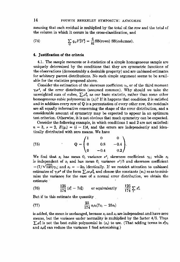
Consider the following example, in which conditions 1 and 2 are not satisfied:n = 3, v = 2, E(y,) = (i - 1)0, and the errors are independently and iden-tically distributed with zero means. We have
1 0 0
(75) Q = 0 0.8 -0.4 .\° -0.4 0.2
We find that z1 has mean 0, variance a2, skewness coefficient -yl; while z3is independent of z1 and has mean 0, variance a2/5 and skewness coefficient- (7/'V125),y; and Z2 =-2z3 identically. If we restrict attention to unbiasedestimates of yiel of the form w,,zvz and choose the constants (wi) so as to mini-mize the variance for the case of a normal error distribution, we obtain theestimate
(76) -(1 7z3) or equivalently 1725 z3
But if to this estimate the quantity25
(77) 174 zlz3(7z,-25Qis added, the mean is unchanged, because z1 and z3 are independent and have zeromeans, but the variance under normality is multiplied by the factor 4/5. ThusEiz3 is not the best cubic polynomial in (zi) to use. (That adding terms in z'1z3and Z1z3 can reduce the variance I find astonishing.)

EXAMINATION OF RESIDUALS 15
If we modify the example by adding a fourth observation, so that n = 4,v = 3, and we still have E(y,) = (i - 1)0, we obtain the following results. Theunbiased estimate of the third moment of the error distribution, based on theunweighted sum _iz3, is (approximately) 0.493_iz3, of which the variance if theerror distribution is normal is 6.590.6. The variance under normality of an un-biased estimate of the form ExwAzt is minimized for the estimate(78) 0.365z3 + 0.57342 + 1.0153 + 2.404z4,of which the variance if the error distribution is normal is 5.48a6. I have notdetermined the cubic polynomial estimate with minimum variance.
Consider now data having a one-way classification, that is, consisting of severalhomogeneous samples of possibly unequal size, from each of which we estimate amean. Condition 1 is satisfied but not condition 2, in general. Let the rth samplebe of size n7, so that Y27n, = n and F_,(n, - 1) = v. Let Fi(.) denote a summa-tion over the values of i for the rth sample. From each sample separately wecan estimate yjal by the sample moment
2~ 3
(79) (rn, - l) (nr - 2)of which the variance under normality is 6nraO6/(nr- 1)(nr - 2). The linearcombination of these estimates that has minimum variance under normality isimmediately seen to be a constant multiplied by the unweighted sum E Z3, whichis thus the best estimate of the form ,,wiz3, and is indeed the best cubic poly-nomial estimate (as can be shown without difficulty).More generally, it is easy to show that the unweighted sum ,$3 is the best
statistic (in the above sense of minimum variance) from the class of weightedsums 1wjz'f, provided that the vector (qii) lies in A, which it does when condi-tions 1 and 2 hold.The statistic 2Yz3 can be derived by a likelihood function argument, as follows.
Express the common error distribution by a Gram-Charlier-Edgeworth expan-sion, differentiate the logarithm of the likelihood function with respect to Yjand then set -y and all other shape coefficients zero, and replace the parameters(Or) and a2 by their maximum likelihood estimates. The resulting expression con-tains _iz32 as well as the lower moments Yizi and Fiz2. Thus _iZ3 is suggestedas a suitable criterion for testing whether ey = 0. But the suggestion does notcarry much weight unless the likelihood function is closely proportional to anormal density function, which may be expected to be the case only when thereis a large amount of information about every parameter Or, so that v/n is closeto 1 and qjj is close to bij for all i and j. The residuals then have nearly equalvariance and are nearly uncorrelated.
4.2. It is-not true that all possible information about the shape of the errordistribution is contained in the residuals. This is illustrated by the case of a row-column cross-classification with k(>2) rows and only 2 columns. The distribu-tion of each residual is symmetrical, the sum of cubes of residuals vanishes
16 FOURTH BERKETEY SYMPOSIUM: ANSCOMBE
identically, and it would seem that no estimate of -yi can be obtained from theresiduals. Let the observations be denoted by yuv, where u = 1, 2, * , k, andv = 1, 2. Then the following.expression(80)
3(k-l)(k-2) E [(Yul - )3 -+ (Yu2 - Y2)3- (Yu1 + Yu2 - 1 - 2)
where g, = k-lEuyu., is an unbiased estimate of yala whose variance depends onthe differences between row means. It is analogous to the variance estimatesgiven by Grubbs [15] and Ehrenberg [8], for the assumption that the errors arenormally distributed with unequal variances in the two columns.
4.3. By analogy with a simple homogeneous sample, one might expect that aneasier test of skewness than the g9 statistic could be obtained by comparing thenumber of positive and negative signs among the residuals. But the followingargument suggests that such a test would be ineffectual. For typical factorialdesigns, if n is large and v somewhat less than n, it seems that the numbers ofpositive and negative coefficients in any column of Q are roughly equal, whereasfor a homogeneous sample they are extremely unequal. A particular and im-portant case of skewness occurs when one error is very much larger in magnitudethan all the others. For the factorial experiment this state of affairs will not berevealed by a sharp inequality in the number of positive and negative signs ofthe residuals.
4.4. The above discussion has concentrated on skewness and the gi statistic,because that topic is conceptually easiest. For the one-way classification, asdefined above, we can establish the optimality of a fictitious statistic close to h,as an estimate of the heteroscedasticity parameter x. From each sample thevariance is best estimated by Fi(,)z2/(nt- 1), and if we assume that this has alinear regression on (,ur - p)a2, fictitiously supposed known, it is easy to showthat the minimum variance estimate of x is
,_ (,. _- a) , z2(81) ir
() (nr - 1) (,Ur. - )2'r
and we obtain h when we replace the quantities that are in fact unknown in thisexpression by their obvious estimates. For the one-way classification, the g2statistic is more difficult to investigate than the g1 statistic, and the f statisticfor nonadditivity is not defined.
5. Examples
5.1. A typical factorial experiment. Yates [21] illustrated the procedure ofanalysis of variance by analyzing some observations from a factorial experimenton sugar beet. All combinations of three sowing dates (D), three spacings ofrows (S) and three levels of application of sulphate of ammonia (N) were tested

EXAMINATION OF RESIDUALS 17
in two replications. The plots were arranged in six randomized blocks, a part ofthe three-factor interaction being partially confounded. The design and yieldsof sugar (in cwt. per acre) are shown in table I, except that the arrangementwithin blocks has been derandomized. (Yates gives the original plan.) Blocks1 to 3 form one replication, blocks 4 to 6 the other; n = 54.
If we are to examine the residuals from such an experiment to check on theappropriateness of the least-squares analysis, we must decide how many effectsto estimate. From Yates' analysis, it appears that the largest effect present is thedifferences between blocks. All three factors, D, S, N, have "significant" maineffects, but their interactions appear to be small. The gross mean square of allthe observations about their mean is 56.19. If just the six block means areestimated, we have v = 48 and the residual mean square = 21.43. When themain effects of the factors are estimated in addition to the block means, wehave v = 42 and the residual mean square = 16.08. If all the two-factor inter-actions are also estimated, we have v = 30 and the residual square = 14.46.When, finally, the three-factor interaction is also estimated, we obtain v = 22and the residual mean square = 13.42, this being the mean square used byYates for gauging the estimated treatment effects.Suppose we stop short at estimating the block means and the treatment main
effects. Then any nonzero interaction effects that occur will contaminate theresiduals. One may surmise that such contamination, if small, will have littleeffect on outliers and less still on the 91, g2 and h statistics, and because of thesharp drop in informativeness of the residuals when v is decreased it would bewise to err on the side of estimating few rather than many treatment effects.A very "objective" method of deciding what effects to estimate for the purposeof calculating residuals would be to decide the matter on the basis of priorexpectation, before any analysis of the data. Another method would be to per-form a full conventional analysis of variance, as Yates does, and then select onlythose effects whose estimates were substantially larger than the residual meansquare, for example, those that were "significant" at the 5 per cent level.Whether this is a good rule I do not know, but it appears not unreasonable.Perhaps for the simpler factorial designs, not highly fractionated or "saturated,"a good compromise procedure would be to estimate the block means and treat-ment main effects in any case, and in addition any substantial or "significant"interactions revealed by the usual analysis of variance.
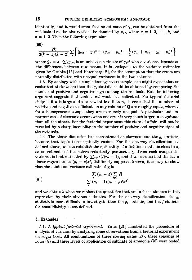
In table I are shown fitted values and residuals for two analyses: (a) onlyblock means estimated, (b) block means and main effects estimated. For (b)these are also shown graphically in figure 1. Analysis (b) is what is indicatedby the above compromise procedure. Consideration is also given below to athird analysis: (c) block means, main effects and two-factor interactions esti-mated. But it has not seemed worthwhile to calculate the residuals for (c). Foranalysis (a), the residuals are contaminated by the main effects of the treat-ments, which seem to be appreciable, and it is noteworthy that the largestresidual, -12.1 in block 1, shrinks to the much less conspicuous value -5.9

18 FOURTH BERKELEY SYMPOSIUM: ANSCOMBE
TABLE I
YIELDS AND RESIDUAL8 OF A FACTORIAL EXPERIMENT
Analysis (a) Analysis (b)
Fitted FittedBlock Treatments Yield Value Residual Value Residual
D S N (yi) (Yi --) (zi) (Yi-y) (zi)
1 0 0 2 50.5 7.3 3.2 10.8 -0.31 0 0 47.8 0.5 6.5 1.22 0 1 46.0 -1.3 7.5 -1.50 1 0 44.6 -2.7 7.1 -2.61 1 1 52.7 5.4 9.9 2.72 1 2 52.2 4.9 7.7 4.40 2 1 51.4 4.1 7.5 3.81 2 2 45.4 -1.9 7.2 -1.82 2 0 35.2 -12.1 1.1 -5.9
2 0 0 0 47.8 8.8 -1.1 8.7 - 1.01 0 1 52.5 3.6 11.5 1.02 0 2 44.1 -4.8 9.3 -5.20 1 1 49.7 0.8 12.1 -2.41 1 2 49.3 0.4 11.7 -2.52 1 0 47.1 -1.8 5.6 1.40 2 2 56.0 7.1 9.4 6.61 2 0 47.2 -1.7 5.1 2.12 2 1 46.2 -2.7 6.1 0.1
3 0 0 1 45.7 -0.2 5.8 3.1 2.51 0 2 43.0 3.1 2.8 0.22 0 0 38.0 -1.9 -3.3 1.30 1 2 50.9 11.0 3.4 7.51 1 0 37.1 -2.8 -0.9 -2.02 1 1 38.2 -1.7 0.1 -1.90 2 0 35.4 -4.5 -3.3 -1.41 2 1 36.5 -3.4 -0.5 -3.12 2 2 34.2 -5.7 -2.7 -3.2
4 0 0 1 39.4 -6.1 5.5 -2.8 2.21 0 0 36.4 2.5 -6.8 3.22 0 2 29.9 -4.0 -5.6 -4.50 1 0 33.3 -0.6 -6.2 -0.51 1 2 33.6 -0.3 -3.2 -3.32 1 1 35.3 1.4 -5.9 1.10 2 2 31.9 -2.0 -5.6 -2.61 2 1 34.4 0.5 -6.4 0.82 2 0 31.3 -2.6 -12.3 3.5
5 0 0 2 33.6 -5.1 -1.3 -1.6 -4.81 0 1 41.8 6.9 -2.5 4.22 0 0 33.2 -1.7 -8.3 1.50 1 1 36.6 1.7 -1.8 -1.61 1 0 33.0 -1.9 -5.9 -1.22 1 2 41.4 6.5 -4.7 6.00 2 0 25.7 -9.2 -8.2 -6.11 2 2 31.4 -3.5 -5.2 -3.42 2 1 37.6 2.7 -7.9 5.5

EXAMINATION OF RESIDUALS 19
TABLE I (Continued)
Analysis (a) Analysis (b)
Fitted FittedBlock Treatments Yield Value Residual Value Residual
D S N (yi) (Y, -Y) (zi) (Y,-) (zj)
6 0 0 0 39.4 -4.7 4.1 -4.9 4.21 0 2 43.1 7.8 -1.8 4.92 0 1 26.6 -8.7 -4.5 -8.90 1 2 36.0 0.7 -1.2 -2.81 1 1 34.2 -1.1 -2.1 -3.82 1 0 33.5 -1.8 -7.9 1.40 2 1 34.9 -0.4 -4.5 -0.71 2 0 32.4 -2.9 -8.5 0.82 2 2 37.7 2.4 -7.3 4.9
under analysis (b). The second largest residual under analysis (a), 11.0 in block 3,becomes the second largest residual, 7.5, under analysis (b). Had there been agross error in one of the observations, it would have been expected to appear asan outlier in both analyses.
Outlier rejection criteria can be calculated from the approximate formula(11.3) of [3], which expresses the premium charged by the rule. For a 2 per centpremium and no prior information about a2, we obtain for analysis (a) the follow-
ZL 10
.15-1 -* * : b 1t
* 0 0*~ ~0
.0
0 0
-15 -IO .-5. 0 5 * 10- ISYl*
0* 0
.0 *@ .
0 ** 0 5
0 *
*~~~~~~~*0l
FIGURE 1
Fitted values and residuals from table I, analysis (b).
20 FOURTH BERKELEY SYMPOSIUM: ANSCOMBE
ing critical value for maxi Izil: 2.86s = 13.2. For analysis (b) the critical valueis 2.69s = 10.8. No rejections are indicated.
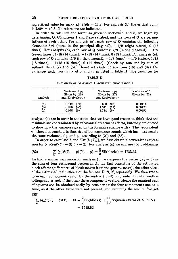
In order to calculate the formulas given in sections 2 and 3, we begin bydetermining Q. Conditions 1 and 2 are satisfied, and the rows of Q are permu-tations of each other. For analysis (a), each row of Q contains the followingelements: 8/9 (once, in the principal diagonal), -1/9 (eight times), 0 (45times). For analysis (b), each row of Q contains: 7/9 (in the diagonal), -1/9(seven times), 1/18 (14 times), -1/18 (14 times), 0 (18 times). For analysis (c),each row of Q contains: 5/9 (in the diagonal), - 1/3 (once), -1/9 (twice), 1/18(18 times), -1/18 (18 times), 0 (14 times). [Check by sum and by sum ofsquares, using (7) and (8).] Hence we easily obtain from (18) and (37) thevariances under normality of g9 and 92, as listed in table II. The variances for
TABLE II
VARIANCES OF STATISTICS CALCULATED FROM TABLE I
Variance of gi Variance of g2 Variance of hGiven by (18) Given by (37) Given by (53)
Analysis and Equivalent n and Equivalent n
(a) 0.142 (39) 0.600 (35) 0.00111(b) 0.210 (26) 1.011 (19) 0.00126(c) 0.698 (6) 3.324 (6) 0.00259
analysis (a) are in error in the sense that we have good reason to think that theresiduals are contaminated by substantial treatment effects, but they are quotedto show how the variances given by the formulas change with v. The "equivalentn" shown in brackets is that size of homogeneous sample which has most nearlythe same variance of g1 and 92, according to (20) and (38).
In order to calculate h and Var [hl(Yi)], we first obtain a convenient expres-sion for _ij(qi,)2(Y, - p)(Yj- y). For analysis (a) we can use (56), obtaining
(82) E(q,,)2(Y - 9)(Y, -) = 8 SS(blocks) = 1733.67.ij ~~~~~~9
To find a similar expression for analysis (b), we express the vector (Yi -y) asthe sum of four orthogonal vectors in A, the first consisting of the estimatedblock effects (differences of block means from the general mean), the other threeof the estimated main effects of the factors, D, S, N, separately. We then trans-form each component vector by the matrix ((qij)2), and note that the result isorthogonal to each of the other three component vectors. Hence the required sumof squares can be obtained easily by considering the four components one at atime, as if the other three were not present, and summing the results. We get(83)
E (qtj)2(Y, -_ )(yj y) = 2 SS(blocks) + 11 SS(main effects of D, S, N)ii 3 18
= 1515.62.
EXAMINATION OF RESIDUALS 21
The same method, a little less easily, yields for analysis (c)(84)
E (q-j) 2( = 3 SS(blocks)-- SS(replications)
+ 23 SS(main effects of D, S, N)
+ 7- SS(two-factor interactions of D, S, N)
= 724.58.
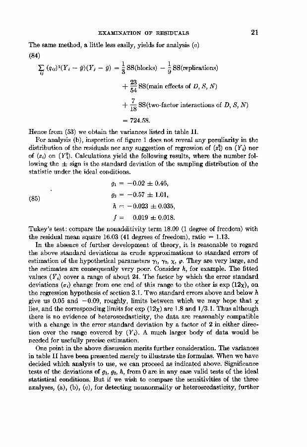
Hence from (53) we obtain the variances listed in table II.For analysis (b), inspection of figure 1 does not reveal any peculiarity in the
distribution of the residuals nor any suggestion of regression of (z2) on (Y1) norof (zi) on (Y2). Calculations yield the following results, where the number fol-lowing the i sign is the standard deviation of the sampling distribution of thestatistic under the ideal conditions.
g = -0.02 i 0.46,
(85) 92 =-0.57 i 1.01,h =-0.023 + 0.035,
f = 0.019 4± 0.018.
Tukey's test: compare the nonadditivity term 18.09 (1 degree of freedom) withthe residual mean square 16.03 (41 degrees of freedom), ratio = 1.13.
In the absence of further development of theory, it is reasonable to regardthe above standard deviations as crude approximations to standard errors ofestimation of the hypothetical parameters yi, 72, X, p. They are very large, andthe estimates are consequently very poor. Consider h, for example. The fittedvalues (Yi) cover a range of about 24. The factor by which the error standarddeviations (aj) change from one end of this range to the other is exp (12x), onthe regression hypothesis of section 3.1. Two standard errors above and below hgive us 0.05 and -0.09, roughly, limits between which we may hope that xlies, and the corresponding limits for exp (12x) are 1.8 and 1/3.1. Thus althoughthere is no evidence of heteroscedasticity, the data are reasonably compatiblewith a change in the error standard deviation by a factor of 2 in either direc-tion over the range covered by (Yr). A much larger body of data would beneeded for usefully precise estimation.One point in the above discussion merits further consideration. The variances
in table II have been presented merely to illustrate the formulas. When we havedecided which analysis to use, we can proceed as indicated above. Significancetests of the deviations of gi, 92, h, from 0 are in any case valid tests of the idealstatistical conditions. But if we wish to compare the sensitivities of the threeanalyses, (a), (b), (c), for detecting nonnormality or heteroscedasticity, further
22 FOURTH BERKELEY SYMPOSIUM: ANSCOMBE
thought is needed) because what each statistic, gi, 92, h, estimates differs for eachanalysis, in accordance with the difference in the implied ideal conditions.
Consider the h statistic. Let us suppose, for the purpose of comparison, thatin fact the (psi) are linear combinations of block means, main effects and two-factor interactions of the factors, but there is no three-factor interaction nor anyother effects on the means; and suppose further that there is a small regressionof error variance on the mean, with parameter x. Then for analysis (c), we obtain(to the best of our knowledge) a nearly unbiased estimate of x by calculating h*,which turns out to be 1.202 h,. (We use the suffices a, b, c here to distinguish be-tween analyses.) But in analyses (a) and (b), some real treatment effects areleft in the apparent error variation, and the result of this seems to be roughly,on the average, to increase the apparent residual variance by a constant amount,independent of the mean; and therefore to diminish the apparent magnitude of x.Hence the following roughly unbiased estimates of x are suggested:
(86) 8sa h* = 1.565 ha s2h* = 1.197 hb.SC c
The variance of each estimate is presumably roughly found by multiplying the
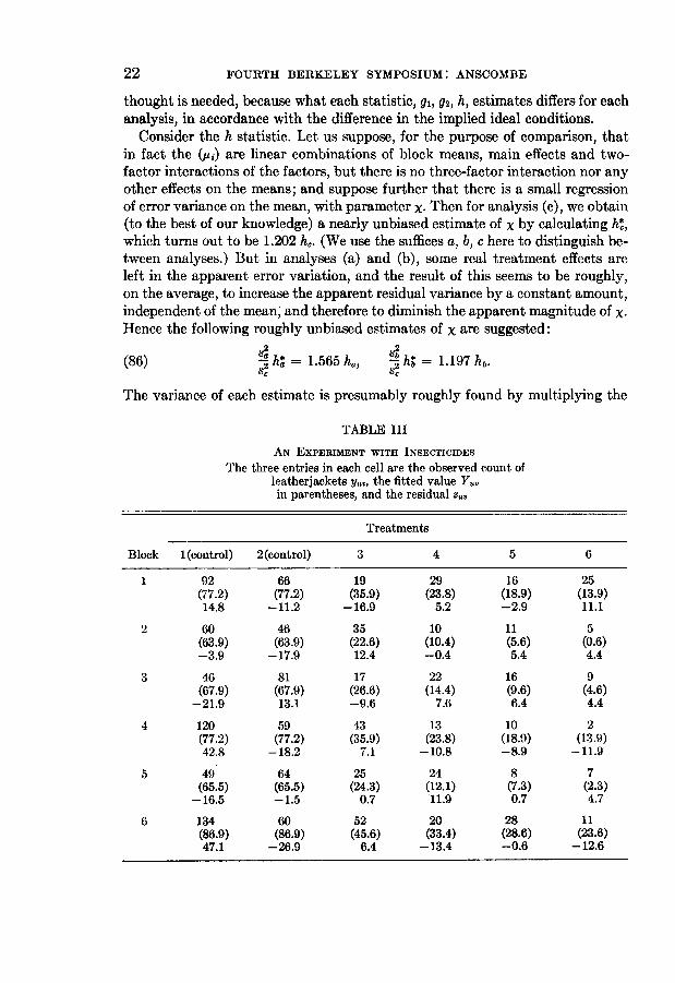
TABLE III
AN EXPERIMENT WITH INSECTICIDESThe three entries in each cell are the observed count of
leatherjackets y.,, the fitted value Y.,in parentheses, and the residual z_
Treatments
Block l(control) 2(control) 3 4 5 6
1 92 66 19 29 16 25(77.2) (77.2) (35.9) (23.8) (18.9) (13.9)14.8 -11.2 -16.9 5.2 -2.9 11.1
2 60 46 35 10 11 5(63.9) (63.9) (22.6) (10.4) (5.6) (0.6)-3.9 -17.9 12.4 -0.4 5.4 4.4
3 46 81 17 22 16 9(67.9) (67.9) (26.6) (14.4) (9.6) (4.6)
-21.9 13.1 -9.6 7.6 6.4 4.4
4 120 59 43 13 10 2(77.2) (77.2) (35.9) (23.8) (18.9) (13.9)42.8 -18.2 7.1 -10.8 -8.9 -11.9
5 49 64 25 24 8 7(65.5) (65.5) (24.3) (12.1) (7.3) (2.3)
-16.5 -1.5 0.7 11.9 0.7 4.7
6 134 60 52 20 28 11(86.9) (86.9) (45.6) (33.4) (28.6) (23.6)47.1 -26.9 6.4 -13.4 -0.6 -12.6

EXAMINATION OF RESIDUALS 23
corresponding entry in table II by the square of the multiplier of h. We obtain(87) (a) 0.0027, (b) 0.0018, (c) 0.0037.While these estimated variances are crude, they are no doubt correct in indicat-ing that analysis (b) is the most sensitive, and analysis (c) the least, for detectinga departure of x from 0.
5.2. Insect counts. To demonstrate that with even a small body of data themethods of this paper are capable of revealing a gross enough violation of theideal conditions, let us consider some leatherjacket counts which Bartlett [5]quoted as an example to illustrate the use of a transformation of the data inreducing heteroscedasticity. In each of six randomized blocks (replications) therewere six plots, four treated by various toxic emulsions and two untreated ascontrols. In table III are shown the total counts of leatherjackets recovered oneach plot, together with the fitted values and residuals when treatment meansand block means are estimated. Let the observation in the uth row and vthcolumn of table III be denoted by yuv, with u, v = 1, 2, * , 6. Then the fittedvalues are given by
Y0 = 62y=.uv + 1XL (Yu1 + Yu2) -(88)
Y = E yuv + 6 E Y. , v _ 3.
The analysis of variance goes as shown in table IV.TABLE IV
ANALYSIS OF VARIANCE FOR EXPERIMENT WITH INSECTICIDES
Degrees of Freedom Sums of Squaxes Mean Squares
Blocks 5 2358.22 471.64Treatments 4 24963.14 6240.78Residual 26 8502.53 327.02
Because there are twice as many control plots as of each type of treated plot)condition 2 is violated. Twelve rows of Q contain the elements: 7/9 (in thediagonal), -2/9 (once), -5/36 (four times), -1/18 (10 times), 1/36 (20 times).The other 24 rows of Q contain: 25/36 (in the diagonal), -5/36 (10 times),1/36 (25 times). It is straightforward to calculate the various functions on Qthat are needed.
E (q*,)2 = 18.833, E (qi,)3 = 12.778,S ~~~~~~~~ii
D = 8.649, F = 0.034,(89)
E (qt,)2(Y ;- Y)(Yj- F) = y8 SS(blocks) +5
SS(treatments)
+ 25 [ 1 E (Yui + Y.2) -
24 FOURTH BERKELEY SYMPOSIUM: ANSCOMBE
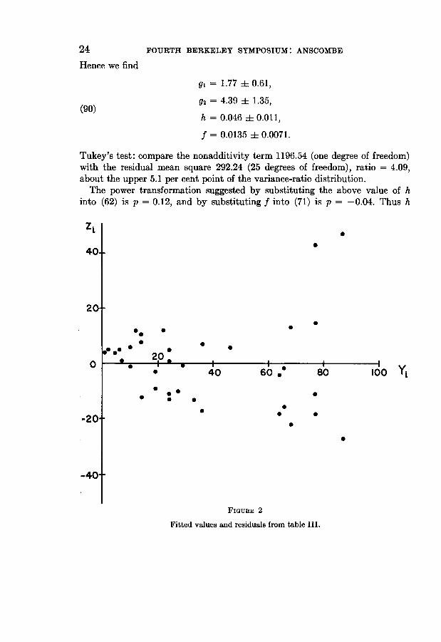
Hence we find
gi = 1.77 -t 0.61,
(90) 92 = 4.39 i 1.35,
h = 0.046 4i 0.011,
f = 0.0135 i 0.0071.
Tukey's test: compare the nonadditivity term 1196.54 (one degree of freedom)with the residual mean square 292.24 (25 degrees of freedom), ratio = 4.09,about the upper 5.1 per cent point of the variance-ratio distribution.The power transformation suggested by substituting the above value of h
into (62) is p 0.12, and by substituting f into (71) is p = -0.04. Thus h
Zlzt 0~~~~~~~~~~~~40.
20-.
20S0~~~_S
0.0
0 * 40 60 80 IOO Y4
-20- *. * 0
-40-.
FIGURE 2
Fitted values and residuals from table III.
EXAMINATION OF RESIDUALS 25
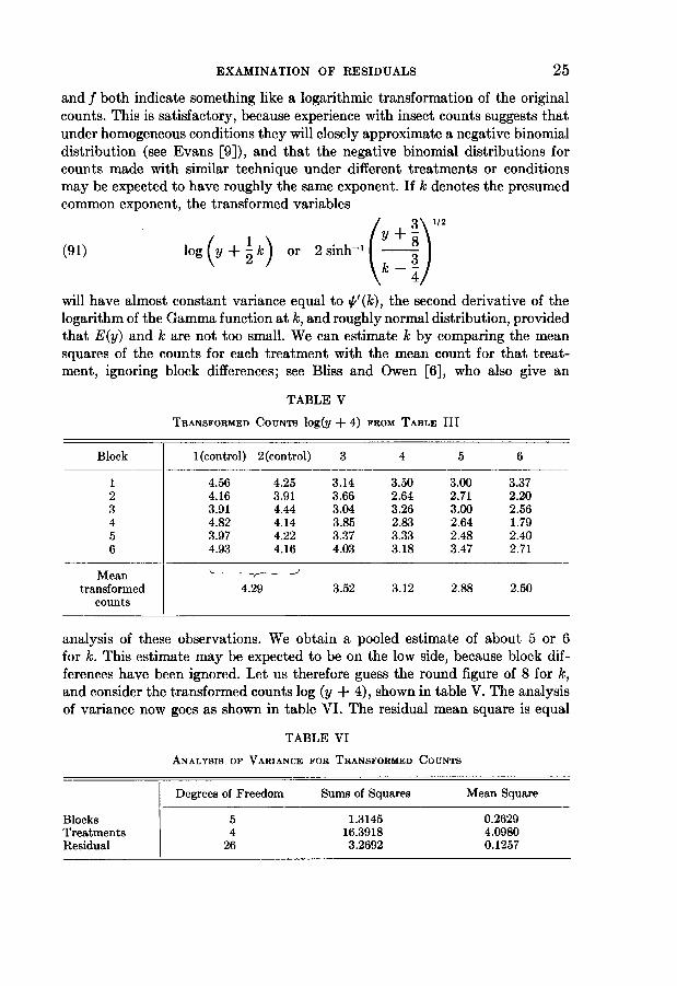
and f both indicate something like a logarithmic transformation of the originalcounts. This is satisfactory, because experience with insect counts suggests thatunder homogeneous conditions they will closely approximate a negative binomialdistribution (see Evans [9]), and that the negative binomial distributions forcounts made with similar technique under different treatments or conditionsmay be expected to have roughly the same exponent. If k denotes the presumedcommon exponent, the transformed variables
(91) log y +I k) or 2 sinh- 8)
will have almost constant variance equal to ik'(k), the second derivative of thelogarithm of the Gamma function at k, and roughly normal distribution, providedthat E(y) and k are not too small. We can estimate k by comparing the meansquares of the counts for each treatment with the mean count for that treat-ment, ignoring block differences; see Bliss and Owen [6], who also give an
TABLE V
TRANSFORMED COUINTS log(y + 4) FROM TABLE III
Block l(control) 2(control) 3 4 5 6
1 4.56 4.25 3.14 3.50 3.00 3.372 4.16 3.91 3.66 2.64 2.71 2.203 3.91 4.44 3.04 3.26 3.00 2.564 4.82 4.14 3.85 2.83 2.64 1.795 3.97 4.22 3.37 3.33 2.48 2.406 4.93 4.16 4.03 3.18 3.47 2.71
Meantransformed 4.29 3.52 3.12 2.88 2.50
counts
analysis of these observations. We obtain a pooled estimate of about 5 or 6for k. This estimate may be expected to be on the low side, because block dif-ferences have been ignored. Let us therefore guess the round figure of 8 for k,and consider the transformed counts log (y + 4), shown in table V. The analysisof variance now goes as shown in table VI. The residual mean square is equal
TABLE VI
ANALYSIS OF VARIANCE FOR TRANSFORMED COUNTS
Degrees of Freedom Sums of Squares Mean Square
Blocks 5 1.3145 0.2629Treatments 4 16.3918 4.0980Residual 26 3.2692 0.1257
26 FOURTH BERKELEY SYMPOSIUM: ANSCOMBE
to 4t'(8.44) approximately, or about 94 per cent of 4'(8), so the guessed valuefor k has been quite well confirmed. The residuals after fitting block and treat-ment means to the entries in table V do not show any interesting phenomena,which is what one would expect with so few observations; and they are not re-produced here. One may conclude that the scale of log (y + 4) is satisfactoryfor viewing the counts through the simple row-column least-squares analysis.(Bliss and Owen recommend for these counts the transformation log (y + 12.6),for reasons that do not entirely convince. Of course, almost any logarithmictransformation will lead to apparently well-behaved residuals, with so few obser-vations.)
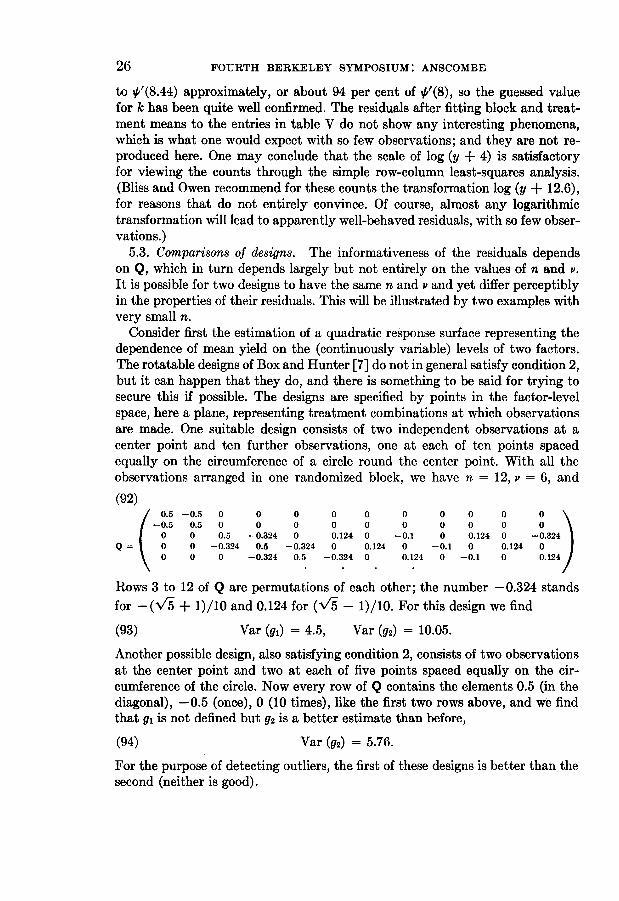
5.3. Comparisons of designs. The informativeness of the residuals dependson Q, which in turn depends largely but not entirely on the values of n and v.It is possible for two designs to have the same n and v and yet differ perceptiblyin the properties of their residuals. This will be illustrated by two examples withvery small n.
Consider first the estimation of a quadratic response surface representing thedependence of mean yield on the (continuously variable) levels of two factors.The rotatable designs of Box and Hunter [7] do not in general satisfy condition 2,but it can happen that they do, and there is something to be said for trying tosecure this if possible. The designs are specified by points in the factor-levelspace, here a plane, representing treatment combinations at which observationsare made. One suitable design consists of two independent observations at acenter point and ten further observations, one at each of ten points spacedequally on the circumference of a circle round the center point. With all theobservations arranged in one randomized block, we have n = 12, v = 6, and(92)
0.5 -0.5 0 0 0 0 0 0 0 0 0 0-0.5 0.5 0 0 0 0 0 0 0 0 0 0 \0 0 0.5 -0.324 0 0.124 0 -0.1 0 0.124 0 -0.324
Q= 0 0 -0.324 0.5 -0.324 0 0.124 0 -0.1 0 0.124 00 0 0 -0.324 0.5 -0.324 0 0.124 0 -0.1 0 0.124
Rows 3 to 12 of Q are permutations of each other; the number -0.324 standsfor -(vK5 + 1)/10 and 0.124 for (V5 - 1)/10. For this design we find
(93) Var (ga) = 4.5, Var (92) = 10.05.
Another possible design, also satisfying condition 2, consists of two observationsat the center point and two at each of five points spaced equally on the cir-cumference of the circle. Now every row of Q contains the elements 0.5 (in thediagonal), -0.5 (once), 0 (10 times), like the first two rows above, and we findthat g1 is not defined but 92 is a better estimate than before,
(94) Var (92) = 5.76.
For the purpose of detecting outliers, the first of these designs is better than thesecond (neither is good).
EXAMINATION OF RESIDUALS 27
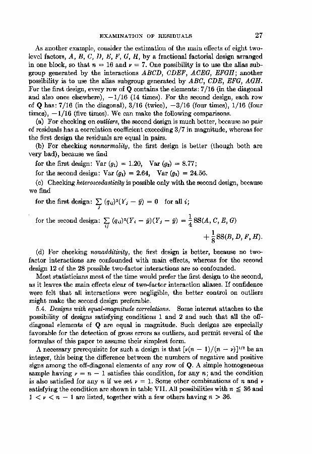
As another example, consider the estimation of the main effects of eight two-level factors, A, B, C, D, E, F, G, H, by a fractional factorial design arrangedin one block, so that n = 16 and v = 7. One possibility is to use the alias sub-group generated by the interactions ABCD, CDEF, ACEG, EFGH; anotherpossibility is to use the alias subgroup generated by ABC, CDE, EFG, AGH.For the first design, every row of Q contains the elements: 7/16 (in the diagonaland also once elsewhere), - 1/16 (14 times). For the second design, each rowof Q has: 7/16 (in the diagonal), 3/16 (twice), -3/16 (four times), 1/16 (fourtimes), - 1/16 (five times). We can make the following comparisons.
(a) For checking on outliers, the second design is much better, because no pairof residuals has a correlation coefficient exceeding 3/7 in magnitude, whereas forthe first design the residuals are equal in pairs.
(b) For checking nonnormality, the first design is better (though both arevery bad), because we find
for the first design: Var (gi) = 1.20, Var (g2) = 8.77;for the second design: Var (gi) = 2.64, Var (g2) = 24.56.(c) Checking heteroscedasticity is possible only with the second design, because
we findfor the first design: E (q.3)2(Y,-9) =0 for all i;
1for the second design: L (qt,)2(Y,- )(Yj-9) = -SS(A, C, E, G)
+ 8 SS(B, D, F, H).
(d) For checking nonadditivity, the first design is better, because no two-factor interactions are confounded with main effects, whereas for the seconddesign 12 of the 28 possible two-factor interactions are so confounded.Most statisticians most of the time would prefer the first design to the second,
as it leaves the main effects clear of two-factor interaction aliases. If confidencewere felt that all interactions were negligible, the better control on outliersmight make the second design preferable.
5.4. Designs with equal-magnitude correlations. Some interest attaches to thepossibility of designs satisfying conditions 1 and 2 and such that all the off-diagonal elements of Q are equal in magnitude. Such designs are especiallyfavorable for the detection of gross errors as outliers, and permit several of theformulas of this paper to assume their simplest form.A necessary prerequisite for such a design is that [v(n - 1)/(n - p)]1/2 be an
integer, this being the difference between the numbers of negative and positivesigns among the off-diagonal elements of any row of Q. A simple homogeneoussample having v = n - 1 satisfies this condition, for any n; and the conditionis also satisfied for any n if we set v = 1. Some other combinations of n and vsatisfying the condition are shown in table VII. All possibilities with n _ 36 and1 < v < n - 1 are listed, together with a few others having n > 36.

28 FOURTH BERKELEY SYMPOSIUM: ANSCOMBE
TABLE VII
POSSIBILITIES FOR DESIGNS WITHEQUAL-MAGNITUDE CORRELATIONS
n vn
9 3, 6 33 11,22,25,2710 5, 8 35 1815 8 36 16,2116 6*, 10* -21 16 49 21, 2825 10, 15 64 8, 28*, 36, 50, 5626 13 81 36, 4528 7, 16, 21, 25 100 45*, 55
It would seem that for most of the listed combinations of n and v thereis no actual design with equal-magnitude correlations. Any ordinary type oforthogonal design has the property that every element of Q is an integermultiple of 1/n. If the design has equal-magnitude correlations, we see that[v(n - )/(n- 1)]112 must be an integer. Possibilities in table VII satisfying thiscondition are shown with the value of v in italics. The asterisk indicates knownsolutions. Solutions for n = 16 were given in [3]. The possibility n = 64 andv = 28 is realizable as a hyper-Graeco-Latin square, formed by superimposingthree orthogonal 8 X 8 Latin squares. The possibility n = 100 and v = 45 issimilarly realizable by superimposing four orthogonal 10 X 10 Latin squares, ofwhich the existence has been demonstrated by R. C. Bose. There is an unlimitedsequence of such Latin square designs having equal-magnitude correlations. Inparticular, they exist whenever n is a power of 4. One may conjecture that thepossibility n = 64 and v = 36, may be realizable by a 26 factorial experimentwith a suitable selection of interactions estimated.
5.5. A counterexample. Not every kind of departure from the ideal statisticalconditions can be seen clearly by examining the residuals (quite apart from theimprecision arising from large sampling errors). A good example of the possibleunhelpfulness of looking at residuals is provided by some data (apparentlyslightly faked) quoted by Graybill [14], showing the yields of four varieties ofwheat grown at 13 locations in the state of Oklahoma. If the residuals from rowand column means are calculated, they seem to have different mean squares inthe four columns, and we might be led to modify the least-squares analysis bypostulating a different error variance for each variety. But if the original observa-tions (not these residuals) are examined more closely, it will appear that thelocations do not have a simple additive effect, but rather the varieties seem torespond with different sensitivity to different locations. Variety number 3 hasnearly the same yield at all locations, whereas the other varieties show pro-nounced differences, on the whole similar in sign but varying in magnitude. Itis primarily the additive assumption about rows and columns which is inap-propriate here, and needs to be modified. A more plausible assumption would

EXAMINATION OF RESIDUALS 29
be the following. The observation y,, in the uth row and vth column, whereu = 1, 2, * * ,13, and v = 1, 2, 3, 4, is independently drawn from a populationwith mean 0, + pu/ci, and variance c2/a2. The parameters (a,) can be estimatedas inversely proportional to the root mean squares of entries in each column ofthe original table: we get the estimates 0.21, 0.36, 1.00, 0.42. If now the entriesin each column are multiplied by the corresponding d, we obtain a set of num-bers in which (as near as we can judge) row and column effects are additive andthe error variance is constant.
6. Discussion
6.1. Given some observations (yi) and associated linear hypothesis, that is,given the matrix A, we can group together under four main headings the variousquestions that can be asked concerning the appropriateness of a least-squaresanalysis.
(i) Are the observations trustworthy?If the answer is yes, we can proceed to challenge the component parts of the
statement of ideal statistical conditions.(ii) Is it reasonable to suppose the (yi) to be realizations of independent chance
variables such that there exist parameter values (Or) such that E(yi) = YrairDr?(iii) Is it reasonable to suppose the (yi) to be realizations of independent chance
variables all having the same variance?(iv) Is it reasonable to suppose the (yi) to be realizations of independent chance
variables all normally distributed?One might add a fifth query concerning the supposition of independence, but
that seems to be a metaphysical matter. A phenomenon which could be thoughtof as one of dependence between chance variables could also be thought of interms of independent chance variables having a different mutual relation. Inmany applications of the method of least squares, independence is a natural as-sumption, either because of the physical independence of the acts of observa-tion, or because of a randomization of the layout. One might add a further, moreradical, query about interpreting the observations as any sort of chance phe-nomena. Why think in terms of chance variables at all? B. de Finetti and L. J.Savage have claimed that it is possible to express all kinds of uncertaintyregarding phenomena in terms of subjective probabilities. To avail ourselves of adistinct physical concept of random phenomena (here referred to by the label"chance") is, they have shown, unnecessary. But the physical concept is never-theless attractive, both because it is philosophically simpler than any. logicalconcept of probability, and because of its familiarity in orthodox statisticalthinking. Be all this as it may, we shall here think exclusively in terms of inde-pendent chance variables. Let us now consider each of the above four types ofquestion in turn.The first question concerns whether we should accept the observations at their
face value, or discard them, partly or wholly. If the general level of the observa-

30 FOURTH BERKELEY SYMPOSIUM: ANSCOMBE
tions, that is, y, or the calculated estimates of some of the parameters (Or), orthe estimate of the error variance a2, are strongly discrepant with our priorexpectations, we shall suspect that a blunder has been made somewhere, incarrying out the plan of observation, or in the arithmetical reduction of theoriginal readings. If the blunder cannot be identified and rectified, the observa-tions will perhaps be rejected altogether. The possibility that occasionally asingle observation is affected by a gross error can be allowed for by examiningthe largest residuals. In some circumstances it will be appropriate to adopt adefinite routine rejection rule for outliers.Under the heading (ii) comes a familiar question. In the analysis of a factorial
experiment, how many interactions should be individually estimated, how manyshould be allowed to contribute to the estimation of the error variance? Is thematrix A big enough, or should further columns (representing interactions) beadded, or conversely, can some columns safely be deleted? Another sort of ques-tion that can arise concerns the scale or units in which the observations canbest be expressed. When what is observed is the yield of a production process,we are usually interested rather strictly in estimating (or maximizing) meanyields, and a nonlinear transformation of the observations might wel[ be con-sidered to be out of place, even if it brought some apparent advantages for thestatistical analysis. But in other cases less easily resolved doubts arise about theproper scale of measurement. If electrical resistance is observed, would it bebetter expressed by its reciprocal, conductivity? If the dimension of objects offixed shape is observed, should a linear dimension be recorded, or its square, orcube? In some population studies we expect treatment effects to be multiplica-tive, and a linear hypothesis about (,ci) becomes more plausible after the countshave been transformed logarithmically. In recording sensory perceptions or valuejudgments arbitrary numerical scores are sometimes used, and on the face of itthese might as well be transformed in almost any manner. We may hope thatby transforming the observations we can arrange that the ideal statistical condi-tions obtain to a satisfactory degree of closeness, for a small parameter set (0,).Tukey's nonadditivity test (f statistic) is valuable as an aid to reducing the num-ber of interactions that need to be considered.Under the heading (iii), the h statistic is designed to show up that kind of
dependence of the error variance on the mean that could be removed by a powertransformation of the observations. Other possible sorts of heteroscedasticity canbe detected by examining the residuals, but they are not studied here.
Question (iv) regarding nonnormality can be examined with the g, and 92statistics.
6.2. The four statistics studied in this paper, 91, g2, h, f, and also the largestresidual, maxi Izil, studied in [3], are by no means independent. If the ideal con-ditions fail in some particular respect, more than one of these statistics mayrespond. For example, if n is not very large and if one observation is affectedby a gross error, gi and g2 are likely to be large, and possibly also f and h if theaffected observation has an extreme mean. Any kind of heteroscedasticity may

EXAMINATION OF RESIDUALS 31
affect both g2 and h. Thus it may be much easier, in a particular case, to assertthat the ideal conditions do not hold, than to say what does and what ought tobe done.
Certainly all five statistics are not equally important or interesting. I suggestthat it is always worthwhile, if computational facilities permit, to make somesort of check for outliers. Perhaps this is the only universal recommendationthat should be made. If we are willing to consider transformations, then f and hbecome interesting. Above we began by considering gi and g2, but that was onlybecause they were conceptually a little simpler than f and h. It seems that onlyfrom a large bulk of data, such as a whole series of experiments in a particularfield, can any precise information be distilled about the shape of the error dis-tribution. For smaller amounts of data, calculating g1 and (especially) 92 is awaste of time. The graphical plotting of residuals against fitted values is nodoubt a good routine procedure, and can be done automatically by a computer.
6.3. Significance tests for theoretical hypotheses. In sections 2 and 3 abovespecial attention was paid to the sampling distribution of the statistics under thefull ideal conditions, so that significance tests of departure from the ideal condi-tions could be made. In [3], on the other hand, it was suggested that the tradi-tional approach to the rejection of outliers through significance tests wasinappropriate, and that choosing a rejection rule was a decision problem similarto deciding how much fire insurance to take out on one's house. The differenceof approach to related problems calls for explanation. What is at issue is therelevance of significance tests in this context.On a previous occasion [2] I have pointed to two very different situations in
which a "null hypothesis" is of special interest, and some sort of test of con-formity of the observations seems to be called for. In the first situation, thereis a certain hypothesis which there is good reason to expect may be almostexactly true. For example, the hypothesis may be deduced from a general mathe-matical theory which is believed to be good, and the observations have beenmade to test a prediction of the theory. Another example would be an experimenton extrasensory perception; most people believe that no such thing as ESPexists and that a "null hypothesis" deduced from simple laws of chance must betrue, whereas the experimenter hopes to obtain observations that do not con-form with this null hypothesis. Yet another example would be a set of supposedrandom observations from a specified chance distribution, derived from pseudo-random numbers, where we might wish to test conformity of the observationswith the nominal distribution. In such situations we wish to know whether theobservations are compatible with the hypothesis considered. It is irrelevant toask whether they might also be compatible with other hypotheses. Usually weare reluctant to try to embed the null hypothesis in a broader class of admissiblehypotheses, defined in terms of only one or two further parameters, such thatone of these hypotheses must be true. If the evidence shows the null hypothesisto be untenable, shows, that is, that we need to think again, we may perhapsconsider patching up the hypothesis by introducing an extra parameter or two,
32 FOURTH BERKELEY SYMPOSIUM: ANSCOMBE
but we look first at some observations to see what sort of modification is needed.If indeed we had a class of admissible hypotheses at the outset, with not toomany nuisance parameters, the likelihood function would be a complete summaryof the observations, and we could make inferences with Bayes' theorem. But inthe situation envisaged there is no small enough class of admissible hypotheses,no intelligible likelihood function, Bayesian inference is not available, and it isnatural to fall back on the primitive significance test, of which Karl Pearson'sx2 test of goodness of fit is the classic example. In such a test a criterion (func-tion of the observations) is chosen, with an eye to its behavior under some par-ticular alternatives considered possible, and the value of the criterion calculatedfrom the data is compared with its sampling distribution under the null hypoth-esis, for a specified sampling rule. (Sometimes it is a conditional distributionthat is considered.) The end result is a statement that the criterion has beenobserved to fall at such and such a percentile of its sampling distribution.Extreme percentiles (or more generally certain special percentiles) are regardedas evidence that the observations do not conform with the null hypothesis. Thistype of analysis of the data is related to a null hypothesis expressed in terms ofchances in the same way, as nearly as possible, as a simple count of observedfavorable and unfavorable instances is related to a universal hypothesis, of thetype "all A's are B's." Such an analysis is not a decision procedure, it does notimply any decisions. We do not necessarily believe a universal hypothesis is truejust because no contrary instances have been observed, nor do we necessarilyabandon a universal hypothesis just because a few contrary instances have beenobserved. Similarly, our attitude towards a statistical hypothesis is not neces-sarily determined by the extremeness of the observed value of the test criterion.The significance test is evidence, but not a verdict. Its function is humble, butessential. The only way that we can see whether a statistical hypothesis (thatis, a hypothesis about physical phenomena, expressed in terms of chances) isadequate to represent the phenomena is through significance tests, or, moreinformally, by noticing whether the observations are such as we could reasonablyexpect if the hypothesis were true. All scientific theories ultimately rest on asimple test of conformity: universal hypotheses are confirmed by noting theincidence of favorable cases, statistical hypotheses are confirmed by significancetests. Any proposal of a class of admissible statistical hypotheses, prerequisitefor the ordinary use of Bayes' theorem, depends for its justification, if it hasone, ultimately on significance tests.The above argument constitutes, I believe, a defense of Fisher's attitude to
significance tests, in his later writings. In [2] I had not realized the importanceof the absence of a class of admissible hypotheses, and was therefore skepticalconcerning orthodox significance tests. In addition to tests of theoretical hypoth-eses, discussed above, for which orthodox significance tests seem to be ap-propriate, and to tests of simplifying hypotheses, as discussed below, it appearsthat there is a third type of situation to which the name test can be reasonably

EXAMINATION OF RESIDUALS 33
applied, as follows. There is a class of admissible hypotheses, and the problemwould be an ordinary one of estimation except that the prior probability ispartly concentrated on a lower dimensional subspace of the parameter space.When we come to use Bayes' theorem, the calculations are of the sort termed asignificance test by H. Jeffreys. In [2] I did not perceive that inference problemsof this type could indeed arise in science; convincing examples have since beengiven by D. V. Lindley (testing for linkage) and L. J. Savage (testing forstatistic acid).
6.4. Simplifying hypotheses. Can it be said that the ideal statistical condi-tions for a least-squares analysis constitute a theoretical null hypothesis of theabove sort, so that to check it we resort to significance tests? Not without someapology. We can hardly claim that we have theoretical reasons for believing theideal conditions to hold. We have seen in section 5 that with small amounts ofdata it is remarkably difficult for the ideal conditions to disprove themselves.No doubt many users of the least-squares method believe that the ideal condi-tions are very nearly satisfied in practice. If that belief is false (in some field ofobservation), significance tests will eventually show it, if enough observationsare made, and then the user must consider whether the discrepancies matter andwhat he ought to do about them. It is a common scientific practice to make bolduse of the simplest hypotheses until they are clearly shown to need modification.That practice is presumably the best excuse for waiting until discrepancies withthe ideal conditions are clearly visible before questioning the ordinary direct useof the method of least squares.The hypothesis that the ideal statistical conditions are satisfied is an example
of what was called in [2] a simplifying hypothesis. We are disposed to act asthough we believed the hypothesis to be true, not because we really do believeit true, but because we should be so pleased if it were. Once we realize this, wesee that significance tests are not strictly relevant, though possibly useful inshaking us from apathy. What is important to know is not whether the observa-tions conform to the simplifying hypothesis, but whether they are compatiblewith seriously different hypotheses that are equally probable a priori. The cor-rect procedure to follow, in order to decide whether the simplifying hypothesisshould be made, seems to be the following. We first examine all available datain various ways, no doubt calculating the values of various test criteria, in orderto form a judgment as to what kinds of departure from the ideal conditionsoccur. Significance tests as such are not useful, but we shall probably wish tohave some idea of the possible sampling variation of our statistics. We then tryto formulate a plausible class of admissible hypotheses, introducing as few extraparameters as possible. If we are lucky, we may feel we can get away with onlyone extra parameter. Let us consider specially this possibility. An instance wouldoccur if we decided that the ideal statistical conditions held very closely providedwe replaced "normal distribution" by "Pearson Type VII distribution"; therewould then be one extra shape parameter, the exponent. Another instance would

34 FOURTH BERKELEY SYMPOSIUM: ANSCOMBE
occur if we decided that the ideal conditions held very closely except for depend-ence of the error variance on the mean, as defined in section 3.1; x would be theone extra parameter.
Let us call the extra parameter 5, so scaled that when a = 0 we have the fullideal conditions. We must now decide how we should proceed if we knew forsure that 6 was substantially different from 0. The answer would depend on theclass of admissible hypotheses, that is, on what a represented. It might be oneof the following: (a) transform the observations and then use ordinary leastsquares, (b) use some kind of weighted least squares, with weights depending onthe residuals and therefore determined iteratively, (c) apply the least-squaresmethod to a nonlinear hypothesis about (Ai), (d) abandon a comprehensiveanalysis of the observations and attempt only a more limited piecemeal analysis.Presumably this procedure would be less attractive than the ordinary least-squares analysis would have been, had we known for sure that a was zero, be-cause of greater computational effort, or because the parameters would be morepoorly estimated, or because the results would be more difficult to state andcomprehend, or because the results would be more modest in scope. If, however,the least-squares method were used when a was not zero, the results would be tosome extent in error and misleading. What we must now do is determine, as wellas we can, the "break-even point," determine how far a must be from zero forthe error in using simple least squares to outweigh the disadvantages attendingthe alternative procedure. (There may be two break-even points, one positive,the other negative, but for brevity we shall speak as though there was one.)Once the break-even point is fixed, it is easy to formulate a well-defined decisionproblem. No doubt our prior opinion about the value of 5 is diffuse, and somesuitable probability distribution, possibly uniform, can be named, it matterslittle what; and some reasonable loss function, possibly quadratic, can benamed-again it matters little what, provided the break-even point is observed.If the total sample information available about a gives us a rather precise esti-mate of 6, then an almost optimum decision rule is to decide in favor of simpleleast squares or the alternative procedure according to -which side of the break-even point the estimate of 5 comes (see [2]).One component of the above train of argument has received some attention in
the literature, namely, to determine how much the results of a simple least-squares analysis are invalidated when a differs from zero. Unfortunately, atten-tion has been paid exclusively to the significance levels of certain tests con-cerning (Or). In most circumstances such tests are inappropriate and ought notto be made.
6.5. To sum up: In sections 2 and 3 we have considered four statistics designedto reveal certain types of departure from the ideal statistical conditions. Informa-tion has been given about their sampling distribution under the "null hypothesis"of the full ideal conditions. That is better than no information at all about sam-pling distributions, and can be directly applied to (approximate) significancetests having merit as complacency removers. Thus a modest contribution has
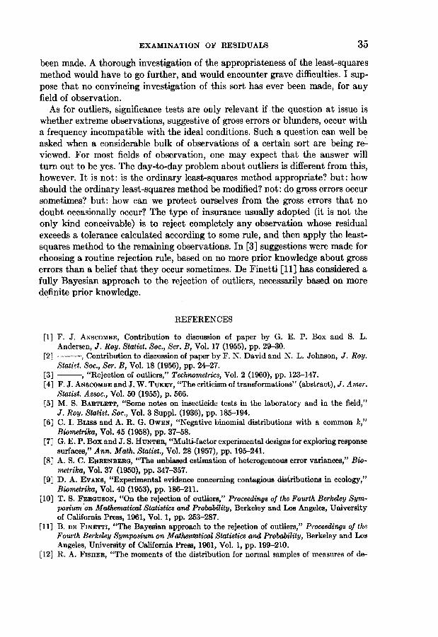
EXAMINATION OF RESIDUALS 35
been made. A thorough investigation of the appropriateness of the least-squaresmethod would have to go further, and would encounter grave difficulties. I sup-pose that no convincing investigation of this sort has ever been made, for anyfield of observation.As for outliers, significance tests are only relevant if the question at issue is
whether extreme observations, suggestive of gross errors or blunders, occur witha frequency incompatible with the ideal conditions. Such a question can well beasked when a considerable bulk of observations of a certain sort are being re-viewed. For most fields of observation, one may expect that the answer willtum out to be yes. The day-to-day problem about outliers is different from this,however. It is not: is the ordinary least-squares method appropriate? but: howshould the ordinary least-squares method be modified? not: do gross errors occursometimes? but: how can we protect ourselves from the gross errors that nodoubt occasionally occur? The type of insurance usually adopted (it is not theonly kind conceivable) is to reject completely any observation whose residualexceeds a tolerance calculated according to some rule, and then apply the least-squares method to the remaining observations. In [3] suggestions were made forchoosing a routine rejection rule, based on no more prior knowledge about grosserrors than a belief that they occur sometimes. De Finetti [11] has considered afully Bayesian approach to the rejection of outliers, necessarily based on moredefinite prior knowledge.
REFERENCES
[1] F. J. ANSCOMBE, Contribution to discussion of paper by G. E. P. Box and S. L.Andersen, J. Roy. Statist. Soc., Ser. B, Vol. 17 (1955), pp. 29-30.
[2] , Contribution to discussion of paper by F. N. David and N. L. Johnson, J. Roy.Statist. Soc., Ser. B, Vol. 18 (1956), pp. 24-27.
[3] , "Rejection of outliers," Technometrics, Vol. 2 (1960), pp. 123-147.[4] F. J. ANSCOMBE and J. W. Tuxzy, "The criticism of transformations" (abstract), J. Amer.
Statist. Assoc., Vol. 50 (1955), p. 566.[5] M. S. BARTLETT, "Some notes on insecticide tests in the laboratory and in the field,"
J. Roy. Statist. Soc., Vol. 3 Suppl. (1936), pp. 185-194.[6] C. I. BLIss and A. R. G. OWEN, "Negative binomial distributions with a common k,"
Biometrika, Vol. 45 (1958), pp. 37-58.[7] G. E. P. Box and J. S. HUNTER, "Multi-factor experimental designs for exploring response
surfaces," Ann. Math. Statist., Vol. 28 (1957), pp. 195-241.[8] A. S. C. EHRENBERG, "The unbiased estimation of heterogeneous error variances," Bio-
metrika, Vol. 37 (1950), pp. 347-357.[9] D. A. EVANS, "Experimental evidence concerning contagious distributions in ecology,"
Biometrika, Vol. 40 (1953), pp. 186-211.[10] T. S. FERGUSON, "On the rejection of outliers," Proceedings of the Fourth Berkeley Sym-
posium on Mathematical Statistics and Probability, Berkeley and Los Angeles, Universityof California Press, 1961, Vol. 1, pp. 253-287.
[11] B. DE FINETTI, "The Bayesian approach to the rejection of outliers," Proceedings of theFourth Berkeley Symposium on Mathematical Statistics and Probability, Berkeley and LosAngeles, University of California Press, 1961, Vol. 1, pp. 199-210.
[12] R. A. FISHER, "The moments of the distribution for normal samples of measures of de-

36 FOURTH BERKELEY SYMPOSIUM: ANSCOMBE
parture from normality," Proc. Roy. Soc. London, Ser. A, Vol. 130 (1930), pp. 17-28.(Reprinted in Contributions to Mathematical Statistics, New York, Wiley, 1950.)
[13] , Statistical Methods for Research Workers, Edinburgh and London, Oliver andBoyd, 1932 (4th ed.), appendix to chapter III.
[14] F. GRAYBILL, "Variance heterogeneity in a randomized block design," Biometrics, Vol. 10(1954), pp. 516-520.
[15] F. E. GRUBBS, "On estimating precision of measuring instruments and product vari-ability," J. Amer. Statist. Assoc., Vol. 43 (1948), pp. 243-264.
[16] P. G. MOORE and J. W. TuKEY, Answer to query 112, Biometrics, Vol. 10 (1954), pp.562-568.
[17] M. E. TERRY, "On the analysis of planned experiments," National Convention Trans-actions 1955, American Society for Quality Control, pp. 553-556.
[18] J. W. TuKEY, "One degree of freedom for nonadditivity," Biometrics, Vol. 5 (1949),pp. 232-242.
[19] , Answer to query 113, Biometrics, Vol. 11 (1955), pp. 111-113.[20] "On the comparative anatomy of transformations," Ann. Math. Statist., Vol. 28
(1957), pp. 602-632.[21] F. YATES, The Design and Analysis of Factorial Experiments, Harpenden, England,
Imperial Bureau of Soil Science (Technical Communication No. 35), 1937, section 10.