examination of multi-seasonal seasonal alos palsar ... · 10.11.2009 3rd alos joint pi symposium,...

10.11.2009 3rd ALOS Joint PI Symposium, Kona, USA 1

Examination of Examination of MultiMulti--SeasonalSeasonal ALOS ALOS PALSAR PALSAR Interferometric CoherenceInterferometric Coherence for Forestry Applications in the for Forestry Applications in the Boreal ZoneBoreal Zone

Christian Thiel, Christiane Schmullius

Friedrich-Schiller-University Jena, Germany


Background


Background

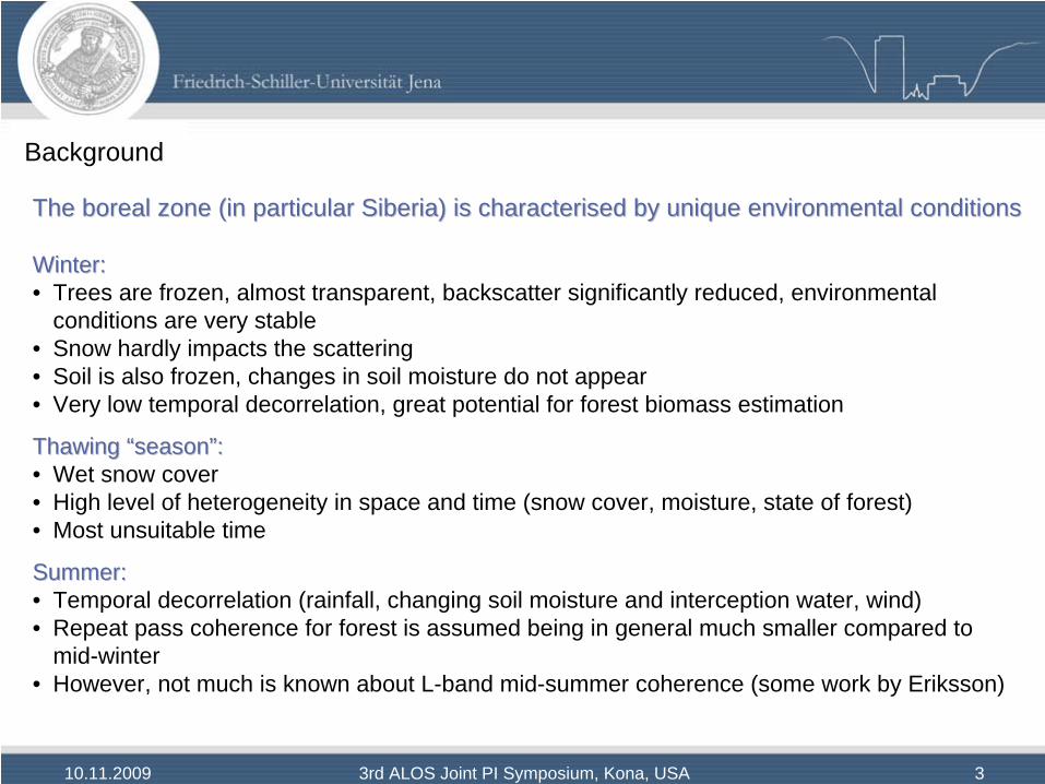
The boreal zone (in particular Siberia) is characterised by uniqThe boreal zone (in particular Siberia) is characterised by unique environmental conditionsue environmental conditions

Winter:Winter:• Trees are frozen, almost transparent, backscatter significantly reduced, environmental

conditions are very stable• Snow hardly impacts the scattering • Soil is also frozen, changes in soil moisture do not appear• Very low temporal decorrelation, great potential for forest biomass estimation

Thawing Thawing ““seasonseason””::• Wet snow cover• High level of heterogeneity in space and time (snow cover, moisture, state of forest)• Most unsuitable time

Summer:Summer:• Temporal decorrelation (rainfall, changing soil moisture and interception water, wind)• Repeat pass coherence for forest is assumed being in general much smaller compared to

mid-winter• However, not much is known about L-band mid-summer coherence (some work by Eriksson)


Outline

1. Introduction1. Test Sites2. SAR Dataset3. Coherence Processing

2. Results1. Methodology of Investigation2. Coherence Images3. Consistency Plots4. Statistics

3. Conclusions and Outlook


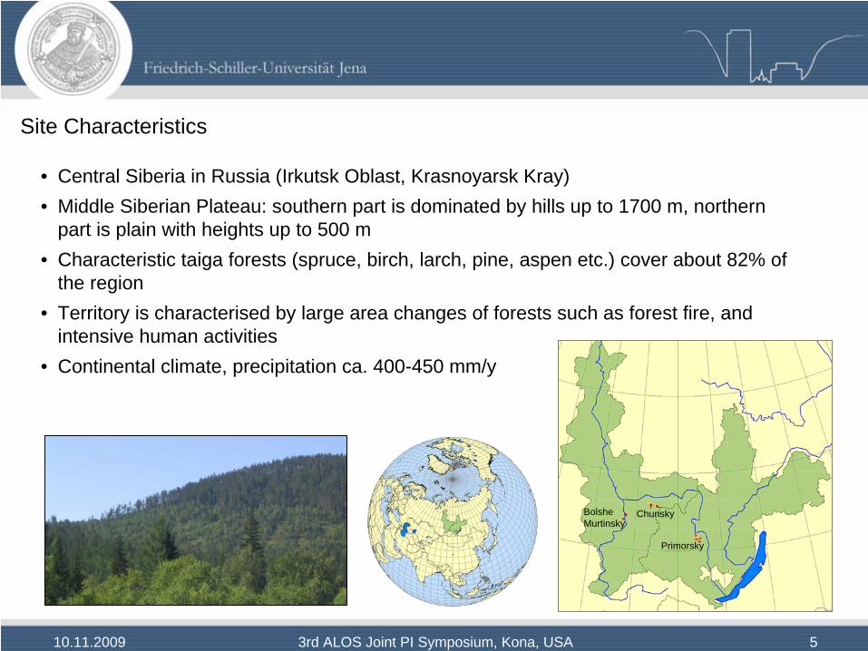
Site Characteristics

• Central Siberia in Russia (Irkutsk Oblast, Krasnoyarsk Kray)• Middle Siberian Plateau: southern part is dominated by hills up to 1700 m, northern

part is plain with heights up to 500 m• Characteristic taiga forests (spruce, birch, larch, pine, aspen etc.) cover about 82% of

the region• Territory is characterised by large area changes of forests such as forest fire, and

intensive human activities• Continental climate, precipitation ca. 400-450 mm/y

BolsheMurtinsky

Chunsky

Primorsky


Local Sites / Forest Inventory Data

Chunsky N (T475/F1150)Chunsky N (T475/F1150)Chunsky E (T473/F1150)Chunsky E (T473/F1150)Primorsky (T466/F1110) N, E, S, WPrimorsky (T466/F1110) N, E, S, WBolshe Murtinsky (T481/F1140) NE, SEBolshe Murtinsky (T481/F1140) NE, SEΣΣ 8 Local sites (> 394 stands per site ) 8 Local sites (> 394 stands per site )

40 km

40 k

m


Ground data

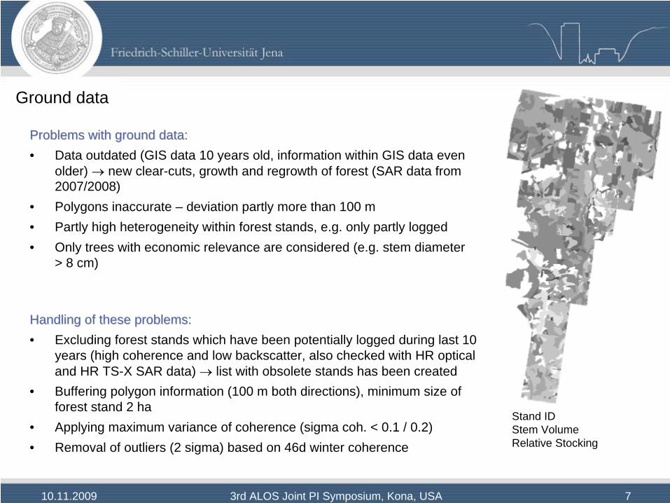
Problems with ground data:Problems with ground data:• Data outdated (GIS data 10 years old, information within GIS data even

older) → new clear-cuts, growth and regrowth of forest (SAR data from 2007/2008)

• Polygons inaccurate – deviation partly more than 100 m• Partly high heterogeneity within forest stands, e.g. only partly logged• Only trees with economic relevance are considered (e.g. stem diameter

> 8 cm)

Handling of these problems:Handling of these problems:• Excluding forest stands which have been potentially logged during last 10

years (high coherence and low backscatter, also checked with HR optical and HR TS-X SAR data) → list with obsolete stands has been created

• Buffering polygon information (100 m both directions), minimum size of forest stand 2 ha

• Applying maximum variance of coherence (sigma coh. < 0.1 / 0.2)• Removal of outliers (2 sigma) based on 46d winter coherence

Stand IDStem VolumeRelative Stocking


Meteorological Data

• Distance between site and the corresponding meteorological station can be more than 200 km

• Typical weather conditions have been observed: Temperatures fare below freezing point during winter and well above freezing point during summer

• Only little precipitation was measured at most acquisition dates

• Wind did not play major role• No remarkable thawing events during winter cycles


SAR DatasetChunsky N (T475/F1150)Chunsky N (T475/F1150) Chunsky E (T473/F1150)Chunsky E (T473/F1150) Primorsky N/E/S/W Primorsky N/E/S/W

(T466/F1110)(T466/F1110)Bolshe NE/SE Bolshe NE/SE (T481/F1140)(T481/F1140)

FBSFBS FBDFBD FBSFBS FBDFBD FBSFBS FBDFBD FBSFBS FBDFBD

30dec0630dec06 18jan0718jan07 28dec0628dec06

14feb0714feb07 05mar0705mar07 12feb0712feb07

20jun0720jun07 02jul0702jul07 21jul0721jul07 15aug0715aug07

05aug0705aug07 17aug0717aug07 05sep0705sep07 30sep0730sep07

20sep0720sep07 02oct0702oct07 21oct0721oct07

17nov0717nov07

05nov0705nov07

21dec0721dec07 31dec0731dec07

05feb0805feb08 02jan0802jan08 21jan0821jan08 15feb0815feb08

22mar0822mar08 17feb0817feb08

07may0807may08

22jun0822jun08 04jul0804jul08 02jul0802jul08

07aug0807aug08 19aug0819aug08 17aug0817aug08

04jan0904jan09 02jan0902jan09

19feb0919feb09 17feb0917feb09

2006

2007

2008

2009


Coherence Computation

• Standard Level 1.1 FBS and FBD were processed to coherence and backscatter

• Interferometric processing consisted of:

- SLC data co-registration to sub-pixel level

- Slope adaptive common-band filtering in range

- Common-band filtering in azimuth

- Image texture (stdev/mean, 15×15 window) was applied to reduce impact of strong scatterers during coherence estimation

- Coherence derivation employs adaptive estimation (variable coherence estimation window sizes): small windows (3×3) at high coherence areas, larger windows (5×5) at low coherence areas

• Coherence orthorectified using SRTM elevation data

• Final pixel spacing: 12.5 m ×

12.5 m (2FBS); 25 m ×

25 m (2FBD, FBS-FBD)


Outline





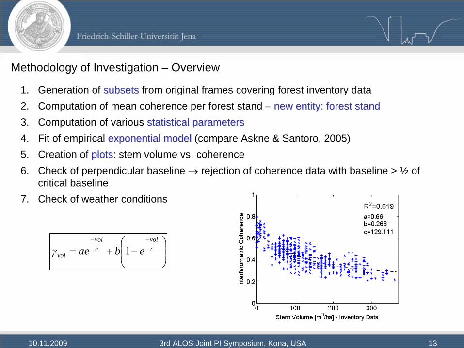
Methodology of Investigation – Overview

1. Generation of subsetssubsets from original frames covering forest inventory data2. Computation of mean coherence per forest stand – new entity: forest standnew entity: forest stand3. Computation of various statistical parametersstatistical parameters4. Fit of empirical exponential modelexponential model (compare Askne & Santoro, 2005)5. Creation of plotsplots: stem volume vs. coherence6. Check of perpendicular baseline → rejection of coherence data with baseline > ½ of

critical baseline7. Check of weather conditions

⎟⎟⎠

⎞⎜⎜⎝

⎛−+=

−−cvol

cvol

vol ebae 1γ


Outline





Coherence Images – Examples Chunsky N – Winter-Winter (Temporal Baseline 46 d)

21dec07_05feb0805nov07_21dec07 05feb08_22mar08

0

1

no stretching applied on image data


Coherence Images – Examples Chunsky N – Winter-Winter (Temporal Baseline 46 d)

21dec07_05feb0805nov07_21dec07 05feb08_22mar08

0

1


Av. coh. = 0.28 Av. coh. = 0.42 Av. coh. = 0.37


Coherence Images – Examples Chunsky N – Winter-Summer

05nov07_20jun0705feb08_20jun07 22mar08_20sep07

0

1



Coherence Images – Examples Chunsky N – Summer-Summer (Temp. Baseline 46 d)

05aug07_20sep0720jun07_05aug07 22jun08_07aug08

0

1


Bperp : 4,060 m (Bc : ~ 6,500 m)


Coherence Images – Examples Chunsky E – Winter-Winter (inter-seasonal)

30dec06_19feb0930dec06_02jan08

0

1



Coherence Images – Examples Chunsky E – Winter-Winter (inter-seasonal)

30dec06_19feb0930dec06_02jan08

0

1


Av. coh. = 0.29 Av. coh. = 0.23


Coherence Images – Examples Chunsky E – Summer-Summer (inter-seasonal)

17aug07_04jul0802jul07_04jul08

0

1



Coherence Images – Examples Chunsky E – Summer-Summer (inter-seasonal)

17aug07_04jul0802jul07_04jul08

0

1


Av. coh. = 0.29 Av. coh. = 0.23


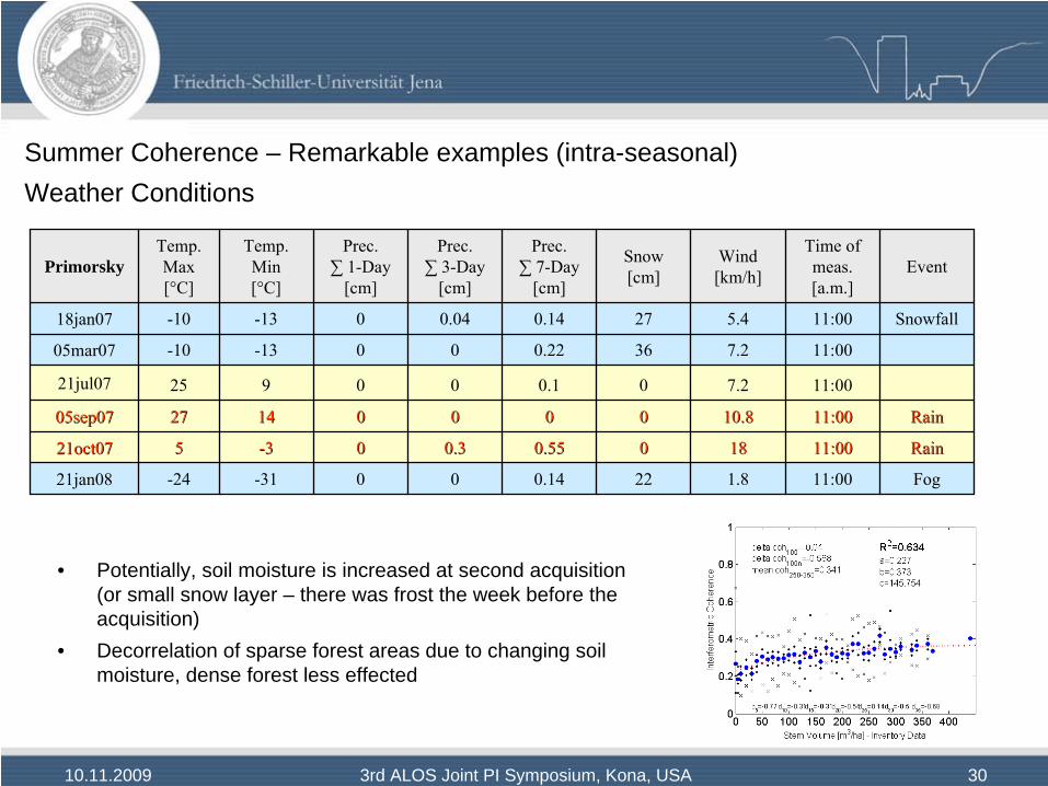
Summer Coherence – Remarkable examples (intra-seasonal)


Summer Coherence – Remarkable examples (intra-seasonal)Bolshe NE (15aug07_30sep07)Primorsky E (05sep07_21oct07)

Primorsky E (21jul07_21oct07)Primorsky N (05sep07_21oct07) Primorsky W (05sep07_21oct07)

Chunsky E (02jul07_02oct07)


Summer Coherence – Remarkable examples (intra-seasonal)Primorsky W (05sep07_21oct07)

Primorsky W (18jan07_05mar07)


Summer Coherence – Remarkable examples (intra-seasonal)Weather Conditions

PrimorskyTemp. Max[°C]

Temp. Min[°C]

Prec.∑

1-Day[cm]

Prec.∑

3-Day[cm]

Prec.∑

7-Day[cm]

Snow[cm]

Wind[km/h]

Time of meas.[a.m.]

Event

18jan07 -10 -13 0 0.04 0.14 27 5.4 11:00 Snowfall

05mar07 -10 -13 0 0 0.22 36 7.2 11:00

21jul07 25 9 0 0 0.1 0 7.2 11:00

05sep0705sep07 2727 1414 00 00 00 00 10.810.8 11:0011:00 RainRain

21oct0721oct07 55 --33 00 0.30.3 0.550.55 00 1818 11:0011:00 RainRain

21jan08 -24 -31 0 0 0.14 22 1.8 11:00 Fog

• Potentially, soil moisture is increased at second acquisition (or small snow layer – there was frost the week before the acquisition)

• Decorrelation of sparse forest areas due to changing soil moisture, dense forest less effected


Outline





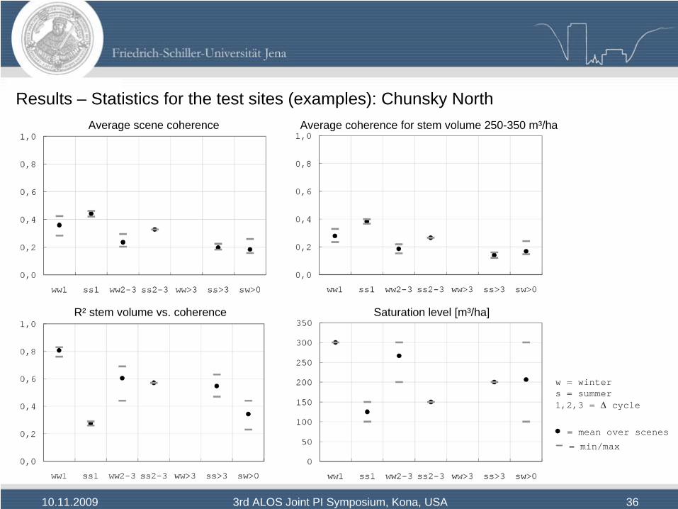
Results – Statistics for the test sites (examples): Chunsky NorthAverage scene coherence Average coherence for stem volume 250-350 m³/ha

R² stem volume vs. coherence

w = winters = summer1,2,3 = Δ

cycle

•

= mean over scenes

- = min/max

Saturation level [m³/ha]


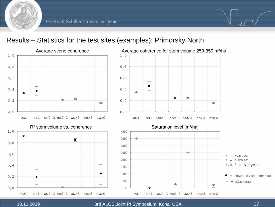
Results – Statistics for the test sites (examples): Primorsky NorthAverage scene coherence Average coherence for stem volume 250-350 m³/ha

R² stem volume vs. coherence Saturation level [m³/ha]


cycle

•

= mean over scenes

- = min/max


Results – Statistics for the test sites (examples): Bolshe Murtinsky NortheastAverage scene coherence Average coherence for stem volume 250-350 m³/ha

R² stem volume vs. coherence


cycle

•

= mean over scenes

- = min/max

Saturation level [m³/ha]


Summary of Statistical Analysis

• For consecutive cycles (temporal baseline = 1 cycle):

• Averaged summer-summer coherence of complete scene and of dense forest in general well exceeds winter-winter coherence

• R² (stem volume vs. coherence) is not driven by mean coherence (of complete scene & dense forest)

• Saturation occurs at very low stem volume for summer-summer coherence and close to maximum biomass for winter-winter coherence

• Increasing stem volume always results in decrease of winter-winter coherence, for summer-summer coherence a reversal of this relationship was observed four times

• At summer-summer coherence generally weak correlation (stem volume vs. coherence) was observed, the spread of coherence measures per stem volume class is much higher than in winter


Summary of Statistical Analysis

• For temporal baseline of 2-3 cycles (intra season):

• Winter-winter coherence in general behaves as the consecutive cycle coherence, average values, R², and saturation are slightly decreased

• Summer-summer coherence also decreases for complete scene and for dense forest, however R², and saturation can improve compared to consecutive cycle coherence

• For temporal baseline of >3 cycles (inter season):

• Winter-winter coherence behaves as above, no remarkable change of average values, R², and saturation

• Summer-summer coherence in general further decreases (for complete scene and for dense forest); R², and saturation can improve or degrade against 2-3 cycles coherence – seemingly strongly dependent on environmental conditions

• Summer-winter coherence, temporal baseline >0 cycles (inter season):

• In general almost complete decorrelation, hardly any practical information – very few images (Chunsky North) could be useful (very low sensitivity to stem volume [only minor slope], yet very low intra-stem-volume-class variation)


Outline





Conclusions – Overall

• ALOS PALSAR data have high potential for forest stem volume estimation in Siberia

• Midwinter FBS coherence provides the most powerful measure

• Summer FBD coherence can provide additional information (e.g. for forest cover mapping), however, temporal baseline must be enlarged to increase temporal decorrelation; →

This approach is very susceptible to variable environmental conditions (weather, soil moisture)

• Computation of coherence based on FBS (winter) and FBD (summer) images is technically feasible but not very useful; it might be used to support forest cover mapping


Conclusions – Summer Coherence Images

• Generally high overall coherence for short temporal baselines if both images are acquired at midsummer →

High coherence also for high stem volume classes – even greater than in winter!

• Weak to no correlation with forest stem volume – spread of coherence measures per stem volume class is much higher than in winter

• Decorrelation increases with increasing temporal baseline, correlation with stem volume can increase with temporal baseline (also matter of environmental conditions)

• Intra- and inter-annual summer coherence can contain helpful information• Decorrelation of 46d coherence appears at patches with (presumably) temporal soil

moisture variations (e.g. headwaters, bogs, floodplains)

• Strong decorrelation, if one of the images is out of season (midsummer)

•• Summer coherence is much less suited for forest stem volume estiSummer coherence is much less suited for forest stem volume estimation than winter mation than winter coherencecoherence


Conclusions – Discussion

• In summer obviously overall temporal decorrelation is not larger than in winter (consecutive cycle coherence)

• This surprisingly seems to apply also to high stem volume classes

• In winter, decorrelation of high stem volume areas is interpreted as effect of volumetric decorrelation, temporal decorrelation is assumed to have minor effect (extremely stable environmental conditions)

• In summer, the decrease of penetration depth into the canopy could result in reduced volumetric decorrelation (raised and narrower scattering centre)

• Evidence in this assumption could be seen in the remarkable examples (increasing coherence with increasing stem volume): →

(potential) change in soil moisture in particular impacts areas with low stem volume

• In summer, larger spread of coherence due to effect of various tree geometries (type etc.)? Do in winter all tree types have the same impact on coherence?


Outlook

• Although many images have been analysed, more effort is required for substantiation of results (increment of time series and number of sites)

• Adaptation of old forestry data by means of growth model

• Investigation of effect of forest type on coherence (in particular on summer coherence)

• Clarification of “high summer coherence phenomenon” →

Investigation of interferometric phase (comparison of winter against summer phase centre)


The End

• Thank you!

Christian ThielFriedrich-Schiller-University Jena, [email protected]

Picture taken near Lake Baikal, 28.09.2009

examination of multi-seasonal seasonal alos palsar ... · 10.11.2009 3rd alos joint pi symposium,...

Documents