1

Exact Asymptotic Goodness-of-Fit

Testing For Discrete Circular Data,

With Applications

David E. Giles

2

1. Background

2. Motivation

3. Existing results

4. Main contribution(s)

5. Overview – main theoretical results

6. Applications

7. Conclusions

3

1. Background

Construction of goodness-of-fit tests when data are distributed on

the circle (sphere, hypersphere) is an important statistical problem.

Tests that have been proposed for continuous data include Kuiper’s

(1959) VN test and Watson’s (1961) 2NU test.

These tests are of the Kolmogorov-Smirnov type, being based on the

empirical distribution function.

Rely on the Glivenko-Cantelli Theorem.

4

5

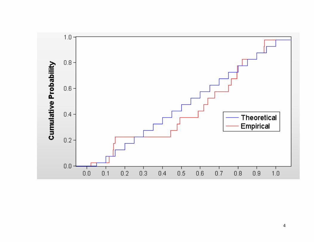
Two general types of test, based on:

1. Maximum “gap” between theoretical and empirical c.d.f.’s.

e.g., Kolmogorov; Kuiper; Watson; Lilliefors.

2. “Area” between the theoretical and empirical c.d.f.’s.

e.g., Anderson-Darling; Cramer – von Mises.

Modify tests if the data are “circular”:

6

0159

7

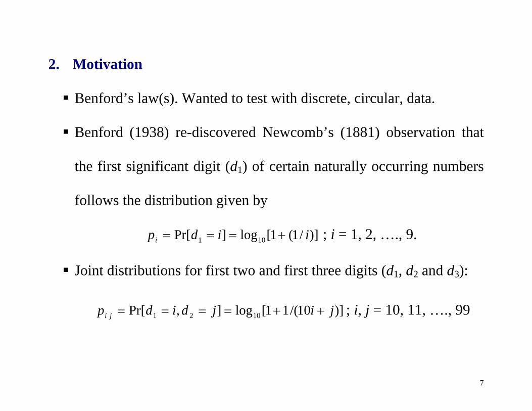
2. Motivation

Benford’s law(s). Wanted to test with discrete, circular, data.

Benford (1938) re-discovered Newcomb’s (1881) observation that

the first significant digit (d1) of certain naturally occurring numbers

follows the distribution given by

)]/1(1[log]Pr[ 101 iidpi ; i = 1, 2, …., 9.

Joint distributions for first two and first three digits (d1, d2 and d3):

)]10/(11[log],Pr[ 1021 jijdidp ji ; i, j = 10, 11, …., 99

8

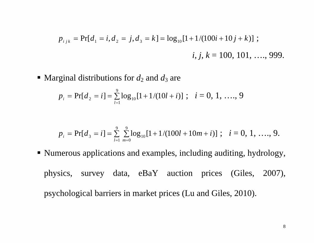
)]10100/(11[log],,Pr[ 10321 kjikdjdidp kji ;

i, j, k = 100, 101, …., 999.

Marginal distributions for d2 and d3 are

9

1102 )]10/(11[log]Pr[

li ilidp ; i = 0, 1, …., 9

9

1

9

0103 )]10100/(11[log]Pr[

l mi imlidp ; i = 0, 1, …., 9.

Numerous applications and examples, including auditing, hydrology,

physics, survey data, eBaY auction prices (Giles, 2007),

psychological barriers in market prices (Lu and Giles, 2010).

9

.04

.08

.12

.16

.20

.24

.28

.32

1 2 3 4 5 6 7 8 9

Benford's First-Digit Law

10

.084

.088

.092

.096

.100

.104

.108

.112

.116

.120

.124

0 1 2 3 4 5 6 7 8 9

BENFORD2BENFORD3

Benford's Second-Digit & Third-Digit Laws

11

3. Existing results

K-S type tests for discrete data have received far less attention in the

literature.

Why is this?

K-S statistics are distribution-free in the continuous case, but

generally not when the data are discrete.

Usual tests have to be modified.

H0: The data follow a discrete circular distribution, F, defined by the

probabilities niip 1}{ . H1: H0 is not true. Sample of N observations.

12

Let niir 1}{ denote the sample frequencies, such that Nr

n

ii

1.

For this general problem, Freedman (1981) proposed a modified

version of Watson’s 2NU test for use with discrete data.

He provided Monte Carlo evidence that this test out-performs

Kuiper’s (1962) modified test for the discrete case.

Freedman’s test statistic is:

]/)[/( 11

211

22*

nj

nj jjN nSSnNU ,

where

ji iij pNrS 1 )/( ; j = 1, 2, …., n.

13

Asymptotic null distribution of the test statistic is a weighted sum of

(n - 1) independent chi-squared variates, each with one degree of

freedom, and with weights which are the eigenvalues of the matrix

whose (i, j)th element is

11

2 ),min()},max({),min()},max({)/( nk ki kjjinpjijinnp .

Freedman expressed the first four moments of the asymptotic

distribution of the test statistic under H0 as functions of these

eigenvalues.

Used these moments to approximate the quantiles of the asymptotic

distribution by fitting Pearson curves.

He only considered the case where the population distribution is

uniform multinomial.

14

4. Main contribution(s)

In fact.....................

Asymptotic null distribution of 2*NU can be obtained directly and

without any approximations by using standard computational

methods.

Specifically, we can use those suggested by Imhof (1961), Davies

(1973, 1980) and others, to invert the characteristic function for

statistics which are weighted sums of chi-squared variates.

There is no need to resort to approximations, curve fitting or

simulation methods.

Davies’ algorithm readily available - e.g., in SHAZAM.

15

This paper demonstrates how to obtain accurate quantiles for 2*NU .

Quantiles are tabulated for discrete uniform, Benford (1st, 2nd, 3rd)

and beta-binomial null distributions.

Several illustrative applications are provided.

Why not simulate the quantiles?

Very inaccurate in tails.

Need to use “rare event” methods such as generalized splitting and

hit-and-run sampling (e.g., Grace and Wood, 2012).

16

5. Main theoretical results

Quantiles for 2*NU asymptotic null distribution, H0: Discrete uniform.

Quantiles for 2*NU asymptotic null distribution, H0: Benford 1st digit.

Quantiles for 2*NU asymptotic null distribution, H0: Benford 2nd digit.

Quantiles for 2*NU asymptotic null distribution, H0: Benford 3rd digit.

Quantiles for 2*NU asymptotic null distribution, H0: Beta-binomial.

Power of 2*NU test.

17

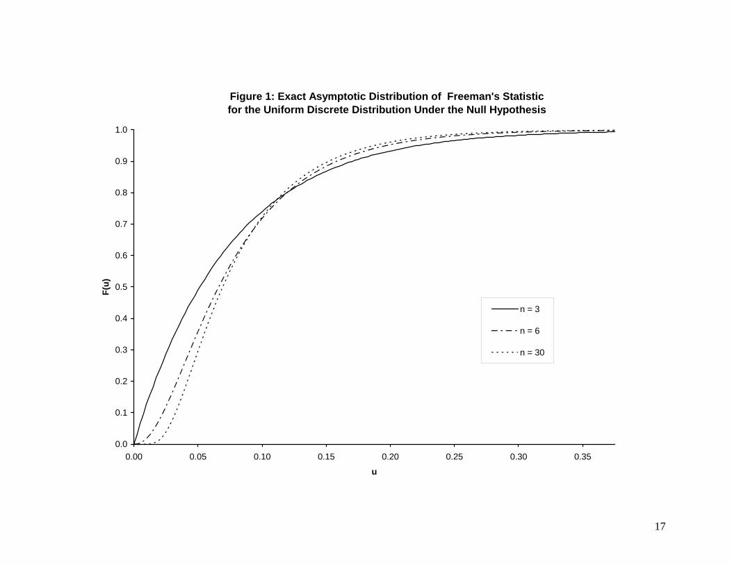
Figure 1: Exact Asymptotic Distribution of Freeman's Statistic for the Uniform Discrete Distribution Under the Null Hypothesis

0.0

0.1

0.2

0.3

0.4

0.5

0.6

0.7

0.8

0.9

1.0

0.00 0.05 0.10 0.15 0.20 0.25 0.30 0.35

u

F(u)

n = 3

n = 6

n = 30

18

Figure 2: Exact Asymptotic Distributions of Freeman's Statistic for Benford's Distributions for First and Second Digits Under the Null Hypthesis

0.0

0.1

0.2

0.3

0.4

0.5

0.6

0.7

0.8

0.9

1.0

0.00 0.05 0.10 0.15 0.20 0.25

u

F(u)

First DigitSecond Digit

Note: Distributions for second and third digits are visually indistinguishable

19

Figure 3: Exact Asymptotic Distribution of Freeman's Statistic forthe Beta-Binomial Distribution With n = 12 Under the Null Hypothesis

0.0

0.1

0.2

0.3

0.4

0.5

0.6

0.7

0.8

0.9

1.0

0.00 0.05 0.10 0.15 0.20 0.25

u

F(u)

alpha = 0.2; beta = 0.25

alpha = 0.7; beta = 0.2

alpha = 2.0; beta = 2.0

alpha = 600; beta = 400

20

6. Applications

Canadian births

Live births, by month, in Canadian Provinces and Territories, 2008.

Demographic literature suggests there will non-uniformity due to

seasonal effects.

Data are circular and discrete (n = 12)

Reject uniformity for Canada as a whole and for all regions except

PEI, NWT, YT and NU.

21

Table 4. Canadian live births, 2008: relative frequency distribution (%)

Month: 1 2 3 4 5 6 7 8 9 10 11 12

NL 7.4 7.4 8.4 7.8 8.8 7.8 8.8 9.7 9.6 8.9 7.8 7.6

PEI 7.3 9.0 9.0 7.6 8.6 8.2 9.6 7.6 8.3 8.4 8.7 7.6

NS 8.3 8.1 8.0 8.1 8.5 8.4 9.5 8.5 8.9 8.5 7.6 7.5

NB 8.0 7.7 8.3 7.7 8.4 8.5 8.7 9.3 9.0 8.5 7.9 7.9

QC 7.7 7.6 8.2 8.2 8.5 8.2 9.2 8.7 9.0 8.9 7.9 7.9

ON 8.2 7.8 8.2 8.4 8.6 8.4 8.8 8.6 8.9 8.6 7.9 7.8

MB 8.2 7.6 7.9 8.1 8.7 8.3 9.0 8.8 8.9 9.0 7.5 8.0

SK 8.2 8.0 8.3 8.2 8.8 8.4 8.7 8.3 9.5 8.3 7.4 7.9

AB 8.0 7.6 8.2 8.4 8.6 8.7 8.9 8.9 8.6 8.4 7.6 8.1

BC 8.0 7.6 8.1 8.2 8.8 8.4 8.9 8.7 8.9 8.4 7.8 8.2

YT 6.2 7.8 9.1 6.4 10.2 6.7 5.9 9.4 10.7 9.1 8.3 10.2

NWT 8.7 7.2 8.6 8.5 9.4 7.8 8.2 10.3 7.9 7.9 8.5 7.1

NU 7.7 7.7 9.3 8.9 9.2 9.6 8.8 8.3 8.7 6.7 7.5 7.6

CAN 8.0 7.7 8.2 8.3 8.6 8.4 8.9 8.7 8.9 8.6 7.8 7.9

22

Table 5. Values of 2*NU . H0: Canadian birth months follow uniform discrete distribution

Province/Territory N 2*NU

NL 4,898 0.771

PEI 1,483 0.038 (Cannot reject @ 75%)

NS 9,188 0.528

NB 7,402 0.490

QC 87,870 6.340

ON 140,791 5.681

MB 15,485 0.994

SK 13,737 0.552

AB 50,856 2.856

BC 44,276 2.093

YT 373 0.089 (Cannot reject @ 30%)

NWT 721 0.052 (Cannot reject @ 50%)

NU 805 0.168 (Reject @ 10%, not at 5%)

CANADA 377,886 18.146

23

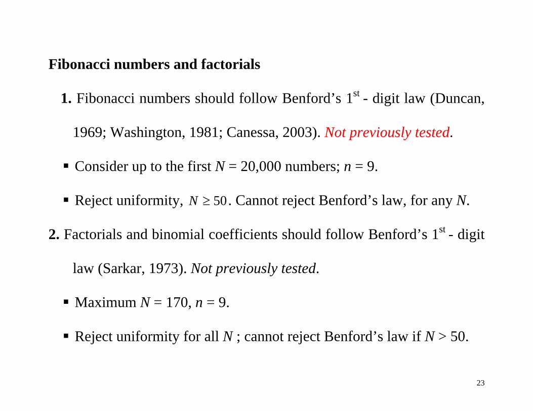
Fibonacci numbers and factorials

1. Fibonacci numbers should follow Benford’s 1st - digit law (Duncan,

1969; Washington, 1981; Canessa, 2003). Not previously tested.

Consider up to the first N = 20,000 numbers; n = 9.

Reject uniformity, 50N . Cannot reject Benford’s law, for any N.

2. Factorials and binomial coefficients should follow Benford’s 1st - digit

law (Sarkar, 1973). Not previously tested.

Maximum N = 170, n = 9.

Reject uniformity for all N ; cannot reject Benford’s law if N > 50.

24

.00

.05

.10

.15

.20

.25

.30

.35

1 2 3 4 5 6 7 8 9 10

BENFORDFIBONACCIFACTORIAL

Benford's First-Digit Law

25

Table 8 (a). Values of 2*NU . H0: Fibonacci first digits follow uniform discrete

distribution; or H0: Fibonacci first digits follow Benford’s distribution

N 2*NU

H0: Uniform discrete H0: Benford

50 0.42831 0.00486

100 0.79613 0.00342

500 3.84342 0.00063

1000 7.71638 0.00042

2000 13.35437 0.00021

5000 38.44199 0.00012

10000 76.8457 3 0.00007

20000 153.54990 0.00003

26

(b). Values of 2*NU . H0: Factorials first digits follow uniform discrete

distribution; or H0: Factorials first digits follow Benford’s distribution

N 2*NU

H0: Uniform discrete H0: Benford

50 1.16915 0.27684

100 1.47179 0.08815

170 1.56025 0.04822

(10% = 0.154; 5% = 0.191; 1% = 0.276)

(10% = 0.143; 5% = 0.179; 1% = 0.263)

27

eBaY auction prices

Price data exhibit circularity. Consider two prices such as $99.99

and $100. Their first significant digits are as far apart as is possible,

yet the associated prices are extremely close.

Giles (2007) considered all of the 1,161 successful auctions for

tickets for professional football games in the “event tickets”

category on eBaY for the period 25 November to 3 December, 2004,

excluding auctions ending with the “Buy-it-Now” option, and all

Dutch auctions.

The winning bids should satisfy Benford’s Law if they are “naturally

occurring” numbers, as should be the case if there were no collusion

among bidders and no “shilling” by sellers in this market.

28

.00

.05

.10

.15

.20

.25

.30

.35

1 2 3 4 5 6 7 8 9

BENFORD1AUCTION1

Auction Price Data - Benford's First-Digit Law

29

.04

.08

.12

.16

.20

.24

0 1 2 3 4 5 6 7 8 9

BENFORD2AUCTION2

Auction Price Data - Benford's Second-Digit Law

30

.0

.1

.2

.3

.4

.5

0 1 2 3 4 5 6 7 8 9

AUCTION3BENFORD3

Auction Price Data - Benford's Third-Digit Law

31

Uniformity is strongly rejected (against non-uniformity) for the first

and third digits, and for the second digit if 250N .

At the 5% significance level, Benford’s Law for the third digit is

unambiguously rejected (against the non-Benford alternative), and

the first digit and second digit laws are also rejected for N > 100.

Suggests that these auction prices are not “naturally occurring

numbers”.

Could be evidence of collusion or “shilling”.

32

Table 9. Values of 2*NU . H0: Football ticket price digits follow uniform discrete

distribution; or H0: Football ticket price digits follow Benford’s distribution

2*NU

Uniform discrete Benford

N Digit 1 Digit 2 Digit 3 Digit 1 Digit 2 Digit 3

50 0.4574 0.1242 0.3952 0.0463 0.1094 0.3883

100 1.1306 0.0476 0.2490 0.0778 0.0195 0.2407

250 3.3508 0.7566 2.7800 0.2673 0.5128 2.7390

500 5.6113 1.1440 4.8389 0.2539 0.6876 4.7680

750 8.3334 1.4935 6.9105 0.3210 0.8473 6.7987

1000 10.6368 2.1118 9.2640 0.2919 1.2482 9.1235

1161 11.7730 2.4803 11.1671 0.2258 1.4664 10.9962

(5%: 0.191373 0.17878 0.19016 0.19052)

33

7. Conclusions

Need to take special care if using EDF tests when data are discrete.

Additional issues if data are also “circular”.

Freedman’s modification of Watson’s 2*NU test is recommended.

Quantiles of null asymptotic distribution can be computed exactly.

Quantiles presented for Uniform, Benford (1, 2, 3) and Beta-

Binomial null distributions.

Various illustrative applications.

The 2*NU test has 100% power, for N 150 when testing nulls of

either Benford’s distribution or beta-binomial distribution, against

uniform alternatives.