evolutionary approaches to solve the 3d ...thermal-aawre floorplanning problem using heterogeneous...
TRANSCRIPT

EVOLUTIONARY APPROACHES TO SOLVE THE 3DTHERMAL-AWARE FLOORPLANNING PROBLEM USING
HETEROGENEOUS PROCESSORS
IGNACIO ARNALDO LUCAS
MÁSTER EN INVESTIGACIÓN EN INFORMÁTICA. FACULTAD DE INFORMÁTICAUNIVERSIDAD COMPLUTENSE DE MADRID
Trabajo Fin Máster en Ingeniería de Computadorescali�cado con SOBRESALIENTE en la convocatoria de Junio 2011
Jueves 16 de Junio de 2011
Directores:
J. Ignacio HidalgoJosé L. Ayala
José L. Risco-Martín

Autorización de difusión
Ignacio Arnaldo Lucas
Jueves 16 de Junio de 2011
El abajo �rmante, matriculado en el Máster en Investigación en Informática de la Fac-ultad de Informática, autoriza a la Universidad Complutense de Madrid (UCM) a difundiry utilizar con �nes académicos, no comerciales y mencionando expresamente a su autor elpresente Trabajo Fin de Máster: �EVOLUTIONARY APPROACHES TO SOLVE THE 3DTHERMAL-AWARE FLOORPLANNING PROBLEM USING HETEROGENEOUS PRO-CESSORS�, realizado durante el curso académico 2010-2011 bajo la dirección de J. IgnacioHidalgo y con la colaboración externa de dirección de José L. Ayala y José L. Risco-Martínen el Departamento de Arquitectura de Computadores y Automática, y a la Biblioteca dela UCM a depositarlo en el Archivo Institucional E-Prints Complutense con el objeto deincrementar la difusión, uso e impacto del trabajo en Internet y garantizar su preservacióny acceso a largo plazo.
Director del proyecto:
J. Ignacio Hidalgo:

Resumen en castellano
La integración en 3D es una técnica prometedora para llevar a cabo el proceso de fab-ricación de futuras arquitecturas multiprocesador. Esta técnica mejora el rendimiento yreduce el cableado obteniendo así un menor consumo global. Sin embargo, la integraciónen 3D provoca problemas térmicos de gran importancia debidos a la mayor proximidad deelementos que irradian calor, acentuando el impacto de los puntos calientes. Los algoritmosde �oorplanning juegan un papel importante en la reducción del impacto térmico, pero notienen en cuenta el per�l dinámico de las aplicaciones. Este trabajo propone un innovador�oorplanner guiado por los pér�les de consumo de potencia de un conjunto de aplicacionesrepresentativas del ámbito de ejecución. Los resultados muestran que tener en cuenta elper�l dinámico de las aplicaciones en vez del los valores en el caso peor lleva a mejorar larespuesta térmica del chip.
Palabras clave
multiprocesador, �oorplanning, restricciones térmicas, per�l dinámico de ejecución, mul-tiobjetivo, algoritmo genético

Abstract
3D integration has become one of the most promising techniques for the integrationfuture multi-core processors, since it improves performance and reduces power consumptionby decreasing global wire length. However, 3D integration causes serious thermal problemssince the closer proximity of heat generating dies makes existing thermal hotspots moresevere. Thermal-aware �oorplanners can play an important role to improve the thermalpro�le, but they have failed in considering the dynamic power pro�les of the applications.This work proposes a novel thermal-aware �oorplanner guided by the power pro�ling of aset of benchmarks that are representative of the application scope. The results show howour approach outperforms the thermal metrics as compared with the worst-case scenariousually considered in �traditional� thermal-aware �oorplanners.
Keywords
multiprocessor, �oorplanning, thermal-aware, pro�ling, multi-objective, genetic algo-rithm

Table of Contents
Índice i
1 Introduction 11.1 Motivations . . . . . . . . . . . . . . . . . . . . . . . . . . . . . . . . . . . . 11.2 Related work . . . . . . . . . . . . . . . . . . . . . . . . . . . . . . . . . . . 31.3 Contributions . . . . . . . . . . . . . . . . . . . . . . . . . . . . . . . . . . . 5
2 Manycore and Heterogeneous architectures 62.1 Manycore architectures . . . . . . . . . . . . . . . . . . . . . . . . . . . . . . 7
2.1.1 Intel's Single-Chip Cloud Computer . . . . . . . . . . . . . . . . . . . 72.2 Heterogeneous architectures . . . . . . . . . . . . . . . . . . . . . . . . . . . 82.3 Proposed architectures . . . . . . . . . . . . . . . . . . . . . . . . . . . . . . 9
2.3.1 OVPsim API's . . . . . . . . . . . . . . . . . . . . . . . . . . . . . . 92.3.2 Core models . . . . . . . . . . . . . . . . . . . . . . . . . . . . . . . . 112.3.3 Simulated manycore heterogeneous architectures . . . . . . . . . . . . 132.3.4 Designing manycore heterogeneous architectures with OVPsim . . . . 142.3.5 Multiprocessor Scheduling Algorithm . . . . . . . . . . . . . . . . . . 17
3 An Evolutionary Algorithm for the 3D Floorplanning problem 203.1 Multi-Objective Evolutionary Algorithms (MOEA) . . . . . . . . . . . . . . 21
3.1.1 SPEA2 . . . . . . . . . . . . . . . . . . . . . . . . . . . . . . . . . . . 233.1.2 NSGA-II . . . . . . . . . . . . . . . . . . . . . . . . . . . . . . . . . . 24
3.2 Common representations . . . . . . . . . . . . . . . . . . . . . . . . . . . . . 253.2.1 Slicing Structures . . . . . . . . . . . . . . . . . . . . . . . . . . . . . 253.2.2 O-trees . . . . . . . . . . . . . . . . . . . . . . . . . . . . . . . . . . . 26
3.3 Proposed Algorithm . . . . . . . . . . . . . . . . . . . . . . . . . . . . . . . 283.3.1 Genetic representation and operators . . . . . . . . . . . . . . . . . . 283.3.2 Fitness function . . . . . . . . . . . . . . . . . . . . . . . . . . . . . . 30
4 Power Pro�ling Phase 314.1 Benchmarks . . . . . . . . . . . . . . . . . . . . . . . . . . . . . . . . . . . . 314.2 Energy pro�les . . . . . . . . . . . . . . . . . . . . . . . . . . . . . . . . . . 34
4.2.1 Memories . . . . . . . . . . . . . . . . . . . . . . . . . . . . . . . . . 354.2.2 Processors . . . . . . . . . . . . . . . . . . . . . . . . . . . . . . . . . 374.2.3 Power pro�les . . . . . . . . . . . . . . . . . . . . . . . . . . . . . . . 37
i

5 Experimental Work 395.1 Experimental Setup . . . . . . . . . . . . . . . . . . . . . . . . . . . . . . . . 395.2 Results . . . . . . . . . . . . . . . . . . . . . . . . . . . . . . . . . . . . . . . 40
5.2.1 Worst Case Scenario . . . . . . . . . . . . . . . . . . . . . . . . . . . 415.2.2 Real power Pro�les . . . . . . . . . . . . . . . . . . . . . . . . . . . . 435.2.3 Performace/temperature tradeo� . . . . . . . . . . . . . . . . . . . . 455.2.4 Results summary . . . . . . . . . . . . . . . . . . . . . . . . . . . . . 54
6 Conclusions and Future Work 56
A Execution distributions 60A.1 30 Cores Architecture . . . . . . . . . . . . . . . . . . . . . . . . . . . . . . . 60A.2 66 Cores Architecture . . . . . . . . . . . . . . . . . . . . . . . . . . . . . . . 62A.3 129 Cores Architecture . . . . . . . . . . . . . . . . . . . . . . . . . . . . . . 64
B Scheduling algorithm 67
ii

Chapter 1
Introduction
As an introduction to our work, we explain the motivations that led us to study this sub-ject. We present the state of the art of the literature related to the �oorplanning problemfocusing both on the techniques and heuristics used and in the 2D and 3D representationsof the elements that compose a chip. In the last section of the introduction we explain thecontributions of our work.
1.1 Motivations
In the last few years semiconductor industry has seen innumerable engineering advancesthat have permitted a logarithmic growth in the capability of integrated circuits (ICs). Thistrend was �rst publicized by Gordon E. Moore in 1965, who suggested that the numberof transistors on an IC doubled every two year (his observation is now known as Moore'sLaw). In fact, huge advances in technology and frequency scaling allowed the majority ofcomputer applications to increase in performance without requiring structural changes orcustom hardware acceleration. While these advances continue, their e�ect on modern ap-plications is not as dramatic as other obstacles such as the memory-wall and the power-wall.
Power density of the microprocessors is increasing with every new process generationsince feature size and frequency are scaling faster than the operating voltage [6]. As aresult, there has been an increase in maximum chip temperatures because power densitydirectly translates into heat. For example, Pentium 4 chips generate more heat than akitchen hotplate. If a Pentium 4 chip is allowed to run without a proper cooling system,it catches �re [2]. Intel's projections show that the heat generated by the processors willincrease sharply in the coming years, approaching that of the core of a nuclear power plant,unless solutions to this problem can be found [1].
The 3D IC is gaining a lot of interest as a viable solution to help maintain the pace ofsystem demands on scaling, performance, and functionality. The bene�ts include system-size reduction, performance enhancement due to shorter wire length, power reduction and
1

the potential for hetero-integration. In the �eld of Multi-Processor Systems-on-Chip (MP-SoCs), only 3D stacks are able to provide the required space for integration. Multiprocessorsystem-on-chips (MPSoCs) are now widely used in application-speci�c systems and high-performance computing. They o�er performance, design and implementation complexity,reduced power consumption, and thermal bene�ts over massively superscalar uniprocessorarchitectures. Nowadays, the primary method of gaining extra performance out of com-puting systems is to introduce additional resources in a single chip. There are two mainapproaches that follow this idea, one of them leads to multicore and manycore homogeneousprocessors which consists in replicating a core several times in a single chip. Multicore andmanycore processors have led to an improvement of the overall performance while reducingthe working frequency. As a consequence, the power dissipation of the chip has remainedin acceptable levels. The other approach introduces specialized resources to achieve speci�ctasks leading to heterogeneous computing systems. This allows a designer to use multipletypes of processing elements, each one able to perform the tasks that it is best suited for. Thecombination of these two approaches is considered to be a future trend in computer design.As a consequence of this combination, new problems emerge such as binary incompatibil-ity, just-in time compilation, the need of e�cient scheduling techniques for heterogeneoussystems etc. Other traditional problems like �oorplanning persist and are more and morerelevant with the increase of computing elements in a single die.
Floorplanning has been proved to be a crucial step in VLSI (Very Large Scale Inte-gration) physical design. In fact, aggressive performance improvements have resulted ina dramatic power consumption increase and a loss of circuit performance and reliability.As explained in [21] MOS current drive capability decreases approximately 4% for every10oC temperature increase, interconnect delay increases approximately 5% for every 10oCincrease while the leakage current increases exponentially with the temperature. Thermalaware �oor planning is �nding an optimum �oor plan by optimizing the cost function con-sisting of area, wire length, and temperature. The objective of the problem is to minimizethe chip area, minimize the wire length, and minimize the maximum temperature of thechip. Thermal aware �oor planning can be used as one of the methods for decreasing themaximum temperature of the chip. Cooling of the blocks in a �oor plan arises due to lateralspreading of heat through silicon blocks [29]. If a hot block is placed besides cooler blocks,lateral spreading of heat takes place. As a result, the temperature of the hot block is reduced.
A common limitation of the previous methods of 3D �oorplanning is that they are fo-cused on area and/or wire length minimization with or without thermal considerations. Thiscan be a serious limitation as modern �oorplanners often have to work with a �xed die sizeconstraint, or with a �xed outline constraint in low-level design of hierarchical �oorplanning�ow [3].
However, all recently developed thermal-aware tools deploy temperature estimation tech-niques only on a single power pro�le representing power pro�les of all inputs and all appli-cations (e.g. using average or peak power pro�le). Di�erent applications lead to di�erent
2

dynamic power pro�les of the blocks. Most of the existing work use either average power orpeak power per block of the applications for simulating temperature, without analyzing theimpact of this assumption.
1.2 Related work
Power consumption has become a critical issue in VLSI physical design. In fact, �oorplan-ning techniques that take thermal data into account are more and more relevant and, as aresult, the �oorplanning problem has become a common research topic. The impact of the�oorplanning on the thermal distribution of real microprocessor-based systems is analyzedin [17], where the placement of components for Alpha and Pentium Pro is evaluated.
Some initial works on thermal aware �oorplanning [8] propose a combinatorial optimiza-tion problem to model our problem. However, the simpli�cation of the considered �oorplanand the lack of a real experimental framework motivated the further research on the area.Thermal placement for standard cell ASICs is a well researched area in the VLSI CADcommunity, where we can �nd works as [7].
In the area of �oorplanning for microprocessor-based systems, some authors consider theproblem at the microarchitectural level [29], where it is shown that signi�cant peak temper-ature reduction can be achieved by managing lateral heat spreading through �oorplanning.
Thermal-aware �oorplanning for 3D stacked systems has also been investigated. Cong[11] proposed a thermal-driven �oorplanning algorithm for 3D ICs, which is a natural ex-tension of his previous work on 2D. In [19], Healy et al. implemented a multi-objective�oorplanning algorithm for 2D and 3D ICs, combining linear programming and simulatedannealing. Recent works as [12] also propose combinatorial techniques to tackle the problemof thermal-aware �oorplanning in 3D multi-processor architectures.
Other works [21] use genetic algorithms to demonstrate how to decrease the peak tem-perature while generating �oorplans with area comparable to that achieved by traditionaltechniques. In �A Slicing Structure Representation for the Multi-layer Floorplan LayoutProblem�, a genetic algorithm is used to solve the multiple layer �oorplanning problem. Itsmain contribution is a three dimensional slicing structure representation. A �oorplan is en-coded in normalized Polish expressions with horizontal, vertical, and lateral cuts. In orderto evaluate a �oorplan, the authors propose to break down the 3D slicing structure. Theyde�ne a slicer algorithm which accepts a 3D �oorplan and the maximum number of layers,and returns a slicing structure for each layer. With this representation, a genetic algorithmis used to minimize whether the overall total area or the balanced area. The advantage ofthis representation is that the crossover and mutation operators are very fast, on the otherhand, polish representations are not suitable for thermal-aware �oorplanning. Nevertheless,slicing structures remain one of the most used representations for the �oorplanning prob-
3

lem. In �Thermal-Aware Floorplanning Using Genetic Algorithms�, Hung et al. present athermal-aware �oorplanning framework based on a genetic algorithm. The main objectiveis to reduce hotspots and to distribute temperature evenly accross a chip while minimizingits area. They de�ne a transfer thermal resistance model and a slicing �oorplan approach isstudied represented by Polish expression. The genetic algorithm proposed aims to minimizethe area needed in the �rst place. Then the algorithm is re-run only with the individualsthat satisfy a good dead space ratio.
Floorplanning techniques evolve as the considered physical constraints change. For ex-ample, a common technique in VLSI is to insert �ip �ops to prevent global wire delayfrom becoming nonlinear, enabling deeper pipelines and higher clock frequency. Therefore,reducing wire delay has become crucial, hence �oorplanning algorithms must take it intoaccount. In the paper �Thermal-aware 3D Microarchitectural Floorplanning�, Ekpanyaponget al. present a �oorplanning algorithm that takes into consideration both thermal issuesand pro�le weighted wire length using mathematical programming. The goal is to minimizethe maximum temperature among all blocks and the overall execution time of a given pro-cessor. In this paper, the �oorplanning problem is presented as a MILP problem. [18] uses asimulated annealing algorithm and an interconnect model to achieve thermal optimization.These works have a major restriction since they do not consider multiple objective factorsin the optimization problem, as opposed to our work. Other works [25] have tackled theproblem of thermal-aware �oorplanning with geometric programming but, in this case, thearea of the chip is not considered constant.
There are other approaches used to study the �oorplanning problem, for example Guoand Takahashi present a genetic algorithm for the VLSI �oorplanning problem using theordered tree (O-tree) representation (see [16]). This representation covers all optimal �oor-plans and has a small search space. Once again, the goal of the genetic algorithm is tominimize the global area and the interconnection cost between the di�erent modules. Thisrepresentation allows to perform operations to the di�erent �oorplans with a reduced com-putational cost.
In our work, we propose to use application pro�ling techniques to guide the �oorplan-ner. A work by [26] shows that the power pro�le does not have major e�ect on the leakagepower as long as the total power remains same. However, they do not consider the e�ectof power pro�le on temperature variation across di�erent applications, especially the peaktemperature of the blocks. Only a recent work [30] incorporates multiple power pro�les in athermal-aware �oorplanner. However, this work is not devoted to MPSoC and could not beeasily extended to 3D multi-processor stacks, where most traditional thermal-�oorplannerfail to �nd an optimal solution.
4

1.3 Contributions
The work presented in this thesis makes the following contributions:
• We adapt the ParMiBench suite to be run on bare machines and simu-
lated with OVPsim to avoid the power overhead caused by an operating system.
• The dynamic profiles of different real world applications are re-
trieved from simulations of manycore heterogeneous architectures
with OVPsim. These pro�les are used to guide a thermal-aware �oorplanner.
• We use a genetic algorithm capable of proposing thermally-optimized
floorplans of architectures composed of 30, 6 and 128 cores. Previousresearch shows that MILP based techniques are unable to propose solutions in thelatter case. The design of this �oorplanner is based on a genetic algorithm capable ofobtaining optimal solutions, in a short time, for a large number of integrated proces-sors and layers and with minimal overhead.
• We propose for a �rst time an efficient thermal-aware 3D floorplanner for
heterogeneous architectures of MPSoCs that uses as input the power tracesobtained during an application power pro�ling phase.
• We obtain different floorplans by targeting different thermal objec-
tives and we evaluate them with real power values retrieved the simulationof 6 di�erent benchmarks.
• We show that considering the worst power consumption does not lead
to optimal floorplans.
5

Chapter 2
Manycore and Heterogeneous
architectures
Nowadays, manycore architectures are a current trend in research. Figure 2.1 shows thedi�erent strategies followed to improve the computers e�ciency while respecting powerand temperature constraints. More and more the di�erent manufacturers tend to designmulticore architectures. It is predicted that this architectures will be heterogeneous withspecial purpose components. This strategy allows to decrease the operating frequency anddesign platforms with a better thermal response.
Figure 2.1: Prediction of Future Trends in Computer Design
6

2.1 Manycore architectures
A manycore processor is one in which the number of cores is large enough that traditionalmultiprocessor techniques are no longer e�cient. It is due to issues with congestion in sup-plying instructions and data to the many processors. The manycore threshold is said tobe in the range of several tens of cores; above this threshold network on chip technology issupposed to be advantageous.
Nowadays there are already several multicore and manycore architectures going from 12to 100 cores architectures. Some of them are already available while others are still in adevelopment phase and correspond to di�erent approaches to multiprocessor architectures.For example, AMD has recently the �Magny-Cours� series, Oracle SPARC T3 (Niagara-3)is widely used in the server segment, Tilera is investing in research to produce the TILEGXchip, �nally Intel's Many Integrated Core Architecture (MIC) is claimed to set the trend indesign for the next years. In this section we study the Intel's Single-Chip Cloud Computerarchitecture and present the architectures studied in this work.
2.1.1 Intel's Single-Chip Cloud Computer
The Single-Chip Cloud Computer initiative is a research stream of Intel's Many IntegratedCore (Intel MIC) project. The �rst Intel MIC products will target applications in HighPerformance Computing (HPC), Workstation, and Data Center segments that use highlyparallel processing. The architecture utilizes a high degree of parallelism in smaller, lowerpower, and single threaded performance Intel processor cores, to deliver higher performanceon highly parallel applications.
The SCC is the second generation processor design that resulted from Intel's Tera-Scaleresearch. It has 24 tiles and two cores per tile. Each core has L1 and L2 caches. The L1caches are on the core; the L2 caches are on the tile next to the core. Each core has a 16KBL1 instruction cache and a 16KB L1 data cache. Each core's L2 cache is 256KB. The SCCcore is a full IA P54C core and hence can support the compilers and OS technology requiredfor full application programming.
Users do not have to run a Linux image on the cores. Running Linux on the cores isthe most common con�guration, but not the only one as some users may be interested inone of the research operating systems being developed for many-core systems. In our case,we propose architectures inspired in this model. This architecture allows to deploy severalapplications in parallel, each one executed by a di�erent group of processors. In this work,we emulate possible task distributions that could be found in the real platforms. In our case,we simulate the benchmarks on bare machines, therefore no operating systems are used.
7

2.2 Heterogeneous architectures
In general, an heterogeneous computing platform consists of processors with di�erent in-struction set architectures (ISA). But this de�nition is usually expanded, in fact, any elec-tronic system that uses di�erent types of computational units is considered heterogeneous.These computational units can be one of the following:
• a general-purpose processor (GPP)
• a co-processor
• a special-purpose processor:
� digital signal processor (DSP)
� graphics processing unit (GPU)
• custom acceleration logic:
� application-speci�c integrated circuit (ASIC)
� �eld-programmable gate array (FPGA)
Heterogeneous architectures are more and more demanded in computing systems. It ismainly due to the increasing need for high-performance and low power systems oriented torun audio, video control and network applications. The level of heterogeneity in moderncomputing systems gradually rises as increases the available chip area caused by the scalingof fabrication technologies. These systems present new challenges not found in typicalhomogeneous systems. The presence of multiple processing elements raises all the issuesinvolved with homogeneous parallel processing systems, while the level of heterogeneity inthe system can introduce non-uniformity in system development and programming practices.The most important problems that need to be solved when dealing with heterogeneousarchitectures are related to:
• Instruction Set Architecture (ISA): computing elements may have di�erent instructionset architectures, leading to binary incompatibility
• Application Binary Interface (ABI): computing elements may interpret memory indi�erent ways. This may include endianness, calling convention and memory layout.It depends both on the architecture and the compiler being used
• Application Programming Interface (API): libraries and operating systems servicesmay not be uniformly available to all computing elements
• Low-Level Implementation of Language Features: language features such as functionsand threads are often implemented using function pointers, a mechanism which re-quires additional translation or abstraction when used in heterogeneous environments
8

• Memory Interface and Hierarchy: computing elements may have di�erent cache struc-tures, cache coherency protocols, and memory access may be uniform or non-uniform(NUMA). Di�erences can also be found in the ability to read arbitrary data lengthsas some processors/units can only perform byte, word, or burst accesses
• Interconnect: computing elements may have di�ering types of interconnections asidefrom basic memory/bus interfaces. This may include dedicated network interfaces,Direct memory access (DMA) devices, mailboxes, FIFOs, scratchpad memories, etc.
Heterogeneous platforms often require the use of multiple compilers to target the di�er-ent types of computing elements found in such platforms. This results in a more complicateddevelopment process compared to homogeneous systems, as multiple compilers and linkersmust be used together in a cohesive way to properly target an heterogeneous platform.Interpretive techniques can be used to hide heterogeneity, but the cost (overhead) of in-terpretation often requires the use of just-in-time compilation mechanisms that result in amore complex run-time system that may be unsuitable in embedded, or real-time scenarios.
Many processors now include built-in logic for interfacing with other devices (SATA, PCI,Ethernet, RFID, Radios, UARTs, and Memory Controllers), as well as programmable func-tional units and hardware accelerators (GPUs, Encryption Co-processors, programmablenetwork processors, A/V encoders/decoders, etc.). Some real world examples are Toshiba'sSpurs Engine used in Sony's Playstation 3, IBM's Cell research project and the recentlyreleased NVIDIA Tegra chip.
2.3 Proposed architectures
We have chosen the OVPsim simulator to achieve our experiments. OVPsim is a multipro-cessor platform emulator that uses dynamic binary translation technology to achieve highsimulation speeds. This simulator provides public API's allowing users to create their ownprocessor, peripheral and platform models. In our case, we have used available processormodels and have designed three di�erent platforms. In this chapter, we explain brie�y theAPI's provided by OVPsim, focusing on the ICM API which is the one that we have used, wealso explain the core models used and �nally, we give a detailed description of the designedarchitectures.
2.3.1 OVPsim API's
The models simulated with OVP are created using C/C++ API's. There are three mainAPI's: ICM, VMI, BHM/PPM.
ICM The ICM API is used for controlling, connecting, and observing platforms. This APIcan be called from C, C++, or SystemC. The platform provides the basic structure of thedesign and creates, connects, and con�gures the components. The platform also speci�es
9
the address mapping, and software that is loaded on the processors. It is very easy withICM to specify very complex and complete platforms composed of:
• di�erent processors
• local and shared memories
• caches
• bus bridges
• peripherals and all their complex address maps
• interrupts and operating systems
• application software
In our case we use only a few functions provided by the ICM API. A detailed explanationof the method followed to build the proposed architectures can be found in 2.3.4. In fact,a simple program that runs a given platform can be made using mainly �ve calls from theICM API:
• icmInit: initializes the simulation environment prior to a simulation run: it shouldalways be the �rst ICM routine called in any application. It speci�es attributes tocontrol some aspects of the simulation to be performed
• icmNewProcessor: used to create a new processor instance
• icmLoadProcessorMemory: Once a processor has been instantiated by icmNewProces-sor, this routine is used to load an object �le into the processor memory. Acceptedformats are ELF and TI-COFF
• icmSimulatePlatform: used to run the simulation of the processor and program, for aspeci�ed duration
• icmTerminate: At the end of the simulation, this function should be called to performcleanup and delete all allocated simulation data structures
VMI For processor modelling there is the VMI API. These API functions provide theability to easily describe the behavior of the processor. A processor model written in Cusing the VMI decodes the target instruction to be simulated and translates it to nativex86 instructions executed on the PC. VMI can be used for modelling 8, 16, 32, and 64 bitarchitectures. There is an interception mechanism enabling emulation of calls to functionsin the application runtime libraries (such as write, fstat etc.) without requiring modi�cationof either the processor model or the simulated application. We are not giving more detailsabout this API as it has not been used in this work.
10

PPM and BHM Behavioral components, peripherals, and the overall environment aremodelled using C code and calls to these two API's. Underlying these API's is an eventbased scheduling mechanism to enable modelling of time, events and concurrency. Periph-eral models provide callbacks that are called when the application software running onprocessors modelled in the platform access memory locations where the peripheral is en-abled. Adding callbacks across memory regions allows memory watchpoints. A callbackis executed whenever there is either a read or write access to a speci�ed range of memoryaddresses. With the given API, the callbacks are created using icmAddReadCallback andicmAddWriteCallback functions. We use these memory callbacks to count memory accesses.
Example
The following code adds a read watchpoint to the address range 0x01000000:0x01000�f :
icmAddReadCallback(processor,0x01000000,0x01000�f,bu�erReadCallBack,0)
The following code adds a write watchpoint to the address range 0x01000000:0x01000�f :
icmAddWriteCallback(processor,0x01000000,0x01000�f,bu�erWriteCallBack,0)
These watchpoints allow the monitoring of memory access behavior of a processor as itruns an application.
2.3.2 Core models
Within OVP there are several di�erent model categories. These models are provided asboth pre-compiled object code and as source �les. Currently there are processor modelsof ARM (processors using the ARMv4, ARMv5, ARMv6, ARMv7 instruction sets), MIPS(processors using the MIPS32 and microMIPS instruction sets), ARC600/ARC700, NECv850, PowerPC and OpenRisc families. There are also models of many di�erent types ofsystem components including RAM, ROM, cache and bridge. There are also peripheralmodels including DMA, UART, and FIFO. There are also models of several di�erent pre-built platforms including software like ucLinux to run on them. One of the main uses ofthe OVP simulation infrastructure is the ability to create and simulate models, either fromscratch, or by using one of the open source models as a starting point. In our case, we usea SPARC model, an ARM model and a PowerPC model.
SPARC
SPARC (from Scalable Processor Architecture) is a RISC instruction set architecture (ISA)developed by Sun Microsystems and introduced in mid-1987. The �Scalable� in SPARCcomes from the fact that the SPARC speci�cation allows implementations to scale fromembedded processors up through large server processors, all sharing the same instruction
11

set. One of the architectural parameters that can scale is the number of implemented reg-ister windows; the speci�cation allows from 3 to 32 windows to be implemented, so theimplementation can choose to implement all 32 to provide maximum call stack e�ciency,or to implement only 3 to reduce context switching time or to implement some numberbetween them. The endianness of the 32-bit SPARC V8 architecture is purely big-endian.The 64-bit SPARC V9 architecture uses big-endian instructions, but can access data ineither big-endian or little-endian byte order, chosen either at the application instruction(load/store) level or at the memory page level (via an MMU setting).
We decide to include SPARC cores in our platforms because it is a commonly usedprocessor in architectures targeting the server segment. On the other hand, these processorshave a high power consumption. Hence, thermal-aware design is mandatory when workingwith these models. As we want to study architectures comparable to the ones predictedto be released in the short term, we need to include processors with di�erent computingpower as well as di�erent power consumptions. In this case, the SPARC cores are the mostpowerful ones but also the hottest elements of our platforms. Therefore, their placement iscrucial to obtain chip con�gurations with an acceptable thermal behaviour.
ARM
ARM is a 32-bit RISC instruction set architecture developed by ARM Holdings. It is knownas the Advanced RISC Machine. The ARM architecture is the most widely used 32-bit ISAin terms of numbers produced. The relative simplicity of ARM processors makes themsuitable for low power applications. As a result, they have become dominant in the mobileand embedded electronics market, as relatively low-cost, small microprocessors and micro-controllers. ARM processors are developed by ARM and by ARM licensees. ProminentARM processor families developed by ARM Holdings include the ARM7, ARM9, ARM11and Cortex. In our case, we do not work with a speci�c core model but with the InstructionSet Architecture (ISA).
This architecture represents the paradigm in embedded design processors. Nowadays itis the most produced architecture and its computing power is increasing in every new gener-ation of processors. We include ARM cores in our architectures because we �nd interestingto mix processor models with very di�erent power consumption. This way, we evaluatethe �oorplanner's ability to strategically place the di�erent cores to avoid hotspots. TheARM cores are also much smaller than the SPARC or the PPC ones. It is also interestingto test how the �oorplanner deals with the di�erent topological constraints of the di�erentprocessor models. In our case, the ARM cores will the medium ones in terms of computingpower.
12

PowerPC
PowerPC (short for Performance Optimization With Enhanced RISC - Performance Com-puting, sometimes abbreviated as PPC) is a RISC architecture created by the 1991 Apple-IBM-Motorola alliance, known as AIM. PowerPC has been renamed Power ISA since 2006but lives on as a legacy trademark for some implementations of Power Architecture basedprocessors. This architecture was originally intended for personal computers, PowerPCCPUs have since become popular as embedded and high-performance processors. PowerPCwas known for being used by Apple's Macintosh lines from 1994 to 2006 but its use in videogame consoles and embedded applications far exceeded Apple's use. PowerPC is largelybased on IBM's earlier POWER architecture, and retains a high level of compatibility withit. In fact, the architectures have remained close enough that the same programs and op-erating systems will run on both if some care is taken in preparation. Newer chips in thePOWER series implement the full PowerPC instruction set. In our case, we do not workwith a speci�c core model but with the Instruction Set Architecture (ISA).
The choice of the PPC cores is justi�ed with the same reasons that led us to studythe ARM cores. We include three di�erent processors with di�erent computing power anddi�erent topological constraints. In this case, the considered PPC model (see 4.2.2) is alsoa low power oriented processor but it is much bigger than the included ARM. The mainreason to include another low power processor is that these two cores will be best suited fordi�erent applications. This means that optimized compilers or operating systems may takeadvantage of this fact and increase both e�cacy and e�ciency of a given platform. Moreover,including low power processors in our platforms allows us to increase the parallelism of theprograms running in our platforms without increasing drastically the temperature of thechip.
2.3.3 Simulated manycore heterogeneous architectures
OVPsim allows the simulation a a variety of platforms. In our case we are interested in thestudy of manycore heterogeneous architectures. The main elements composing our archi-tectures are processors and memories. In fact we will study three di�erent cases that di�erfrom one to another in the number of cores. In all of the cases, there is a shared mem-ory common to all the processors (used for the inter-processor communication) and a localmemory for each of the cores. The proposed platforms are inspired in the Intel's Single-ChipCloud Computer project but we include low power cores that might lead to colder chips.This is a signi�cative change and implies extra di�culties such as di�erent Instruction SetArchitectures and endianness among others.
The platforms considered are heterogeneous, composed of SPARC, ARM and PowerPCprocessors. We are interested in discovering whether this kind of architectures are feasiblesolutions when we scale up the number of cores. We design the di�erent platforms to com-pare the thermal behavior of architectures with di�erent degrees of heterogeneity.
13

In the smallest architecture there are 30 cores with the following distribution: 20 SPARC,5 ARM and 5 PPC. This case corresponds to a multicore platform with a high proportion ofSPARC cores. Therefore the �oorplanner does not have much freedom to place the hottestelements as far away from each other as possible. The most promising strategy is to placethe SPARC cores in the borders of the chip and in the outer layers. This case correspondsto architectures that target the server or HPC segments including special purpose units (thelow power processors in our case) that allow to reduce the heat produced by the chip.
The medium platform is composed of 22 SPARC, 22 ARM and 22 PPC adding up atotal of 66 cores. In this case there is an homogeneous number of the di�erent core models.It is interesting to see how the �oorplanner deals with the hottest elements (SPARC) witha higher degree of freedom. There are already platforms designed within this range of cores.The higher the number of cores, the highest is the need to include low power processors.In fact, homogeneous chips with a high number of SPARC cores present dramatic hotspotsthat can only be solved by adding extra area to separate the cores as much as possible.
Finally, in the last scenario, there are 129 cores: 43 SPARC, 43 ARM and 43 PPC .This case correspond to a scaled up version of the 66 processors architecture. We considerthe study of this case very important as it corresponds to the predicted trend in computerdesign in the short term. There are already projects like Intel's SCC due in the next yearsthat implement a similar number of cores. The higher the number of cores, the harder isto �nd solutions for the �oorplanner. It is due to the fact that the search space increasesexponentially with the number of considered elements. A problem of such a dimensionforces us to research new �oorplanning techniques and algorithms. In fact, for problems ofthis size, traditional thermal-aware techniques fail to return solutions with an acceptablethermal response in a reduced response time. Therefore considering this case represents achallenge and �nding acceptable solutions is one of the contributions of this work.
In our platforms, each processor has its own local memory. To allow communicationbetween processors, we adopt a shared memory strategy. The size of the local memoriesmust be small, as manycore architectures with big local memories are not feasible. On theother hand the size of the shared memory depends on the architecture as more processorsneed a larger memory space to communicate and share data. The exact size of the memoriesconsidered is �xed later on with pro�ling techniques (see section 4.2.1).
2.3.4 Designing manycore heterogeneous architectures with OVP-sim
In this subsection, we explain in detail the procedure followed to build the proposed ar-chitectures with OVPsim. We show the main steps and the di�erent calls to the OVPsimAPI.
14

1. In the �rst place we must de�ne the macros for each memory callback. For example,the memory callbacks of the shared memory are de�ned as follows:
• static ICM_MEM_WRITE_FN(watchWriteCBShared) {writesShared++; }• static ICM_MEM_WATCH_FN(watchReadCBShared) {readsShared++; }
2. we initialize OVPsim, enabling verbose mode to get statistics at end of execution withthe following function call:
• icmInit(ICM_V ERBOSE|..., NULL, 0);
3. we create an array of pointers to processor instances:
• icmProcessorP processor[num_processors];
4. we create the shared memory:
• icmMemoryP shared = icmNewMemory(�shared�, ICM_PRIV_RWX, 0x1���f);
5. we create MMC to perform endian swap needed to hide the endianness problem:
• icmAttrListP icmAttrListMMC = icmNewAttrList();
• const char * string_mmc =icmGetVlnvString (�mmc�,�endianSwap�,...);
• icmMmcP icmMmcP_mmc = icmNewMMC(�swap1�,string_mmc,...);
6. we create bus from the MMC to the shared memory for the PPC's:
• icmBusP busMmcIn = icmNewBus(�busMmcIn�, 32);
• icmBusP busMmcOut = icmNewBus(�busMmcOut�, 32);
7. MMC input/output bus:
• icmConnectMMCBus(icmMmcP_mmc, busMmcIn,�sp1�,0);
• icmConnectMMCBus(icmMmcP_mmc, busMmcOut,�mp1�,1);
8. MMC output bus to shared memory:
• icmConnectMemoryToBus(busMmcOut, �mpswap�, shared, 0xa0000000);
9. create each of the processor models, we show the case of the ARM model:
• const char *armModel = icmGetVlnvString(�arm.ovpworld.org�, �processor�,�arm�,);
• const char *armSemihost = icmGetVlnvString( �arm.ovpworld.org�,�armNewlib�);
10. We set the attribute list for the ARM:
• icmAttrListP icmAttr = icmNewAttrList();
15
• icmAddStringAttr(icmAttr, �variant�, �Cortex-A9�);
11. for each of the processors:
• processor[i] = icmNewProcessor(cpuName, // CPU name�arm�, // CPU typei, // CPU cpuId0, // CPU model �ags32, // address bitsarmModel, // model �le�modelAttrs�, // morpher attributesSIM_ATTRS, // attributesicmAttr, // user-de�ned attributesarmSemihost, // semi-hosting �le�modelAttrs� // semi-hosting attributes);
• create one bus for each processor instantiation:icmBusP bus = icmNewBus(busName, 32);
• connect the processor onto the bus:icmConnectProcessorBusses(processor[i], bus, bus);
• create memories: the ARM processor toolchain sites code in lower memory andstack in higher memory, so we use two memories as a consequence of the defaultlinker script used:icmMemoryP locala = icmNewMemory(localaName, ICM_PRIV_RWX, 0x9���f);icmMemoryP localb =icmNewMemory(localbName,ICM_PRIV_RWX,0x0���f);
• connect local memories onto individual processor bus:icmConnectMemoryToBus(bus, �mp1�, locala, 0x00000000);icmConnectMemoryToBus(bus, �mp1�, localb, 0xf0000000);
• connect the shared memory onto the local bus, this makes it available to allprocessors at the speci�ed address in this case, but it could be at any address ineach processors address map:icmConnectMemoryToBus(bus, mpName, shared, 0xa0000000);
• load an executable �le to the processor local memory, the �le loaded depends onthe processor id:icmLoadProcessorMemory(processor[i], �bitcntsParallelArm.ARM7.elf �,False,False,True))
12. the same method is used to declare and link the other processor models
It is important to note that we connect all the processor buses onto the shared memoryin the same address range, this way the shared memory is available to all the processorsat the same address range. An issue that must be solved when dealing with this kind of
16

heterogeneous architectures is the endianness. In fact, the chosen processor models havedi�erent endianness which makes communication between them impossible. The ARMmodel is only available in an little-endian architecture while the PPC model is only availablein a big-endian architecture. On the other hand, the SPARC model can access data in eitherbig-endian or little-endian byte order. In the case of the PowerPC processors, we use endianswappers between the processors buses and the shared memory. We must also use bridges tomake clear which address range must be connected to the local memory and which addressrange must be connected to the endian swapper. This way, the endianness problem can beignored from now on. In fact, the software running in this architectures does not need tocare about this problem as it is solved with hardware components.
In �gure 2.2, we show a representation of an heterogeneous architecture created followingthe ideas just explained. This heterogeneous architecture is composed of:
• nine processors: three SPARC, three ARM and three PowerPC
• their corresponding local memories divided in two regions: the code is located in lowermemory and stack is located in higher memory
• a shared memory
• an endian swapper, only used by the PowerPC processors
• bus bridges for the PowerPC processors
Another issue is related to the toolchains available that allow us to cross-compile agiven code to be executed in di�erent targets. In fact, these toolchains have pre-establishedmemory addresses for the code, data, etc. Therefore we have to map the processor buses tothese memory regions if we want to make an e�cient use of the memories.
2.3.5 Multiprocessor Scheduling Algorithm
With the OVPsim software, it is possible to simulate multiprocessor platforms. In fact, anynumber of processors can be instantiated within an ICM platform. Shared memory resourcesand callbacks on mapped memory regions are used to allow communication between them.
The provided function icmSimulatePlatform implements the following multiprocessorscheduling algorithm:
1. Simulation time is broken into time slices. By default, each time slice is 0.001 seconds(one millisecond)
2. The simulator selects the �rst processor and simulates it for one time slice. First, thenumber of instructions that should be executed by that processor in a time slice iscomputed, and then the processor is simulated for that number of instructions. Thenumber of instructions in a time slice is:(processor nominal MIPS rate) × 1e6 × (time slice duration)
17

ARM
SPARC
PPC
SWAPPER
ARM
ARM
PPC PPC
SPARC
SPARC
SHARED MEM
Figure 2.2: Example of heterogeneous architecture
3. When the �rst processor has simulated the corresponding instructions, it is suspendedand the next processor is simulated for the time slice
4. When all the processors have simulated the time slice, simulated time is moved on andthe next slice is started
This algorithm is an approximation designed to give realistic simulation results with highsimulator performance: the simulator is not designed to be cycle accurate. The simulationalgorithm is con�gurable by changing the time slice or changing the processor nominal MIPSrate. OVPsim allows us to set these parameters:
• Bool icmSetSimulationTimeSlice(icmTime newSliceSize). Shorter time slices may ap-proximate real system behavior more closely, but degrade simulator performance
• The nominal MIPS rate for each processor can be set with an attribute.
To obtain realistic power pro�les of heterogeneous platforms, we have chosen three pro-cessors with a di�erent computing power, which is a common situation when dealing withthis kind of architectures. Therefore the MIPS rate is set accordingly to the computingpower of each processor. As a result the processor with a higher MIPS rate is the SPARCcore (120), followed by the ARM (80) and the PPC (60). In fact, we are specially interested
18

in understanding the e�ect of synchronization and communication in the temperature ofthe chip. Figure 2.3 shows a typical power dissipation pattern of three di�erent processorsworking together. We can see clearly how the activity of the SPARC core changes periodi-cally over time, waiting for slower processors. This kind of behavior leads us to think thatconsidering always the highest power consumption for each element may lead to an overesti-mation of the dissipated power and temperature of the chip. Therefore, taking into accountthe data retrieved in the proposed power pro�ling phase will lead to better �oorplans.
Figure 2.3: Common power consumption pattern caused by synchronization
OVPsim also allows us to write our custom scheduling algorithm in case the standardmultiprocessor scheduling algorithm does not do what it is required. A custom algorithmcan be built around calls to icmSimulate for each processor. This function will simulatea speci�ed processor for an exact number of instructions. In our case, we need to retrievepro�ling data that is not provided by OVPsim's standard statistical engine. Therefore, weneed to implement our own multiprocessor scheduling algorithm. In particular, the data weneed to obtain is:
• for each simulation window:
� for each processor:
∗ the amount of executed instructions∗ the amount of idle cycles
� for each memory (local and shared):
∗ the amount of read accesses∗ the amount of write accesses
The algorithm proposed is a round robin based scheduling strategy. The detail of thisalgorithm can be seen in the appendix B. The benchmarks chosen for this work are presentedin Chapter 4, as well as the task distributions decided for the di�erent platforms.
19

Chapter 3
An Evolutionary Algorithm for the 3D
Floorplanning problem
Floorplanning has been proved to be a crucial step in VLSI (Very Large Scale Integra-tion) physical design. Traditionally, its main objective has been to minimize the total arearequired to place all of the functional blocks on a chip. The �oorplanning problem is ageneralization of the quadratic assignment problem, which is an NP-hard problem. Thedi�erent approaches to this problem can be divided into three general cases: constructive,knowledge-based, and iterative. The constructive approach starts from a seed module, andadds modules to the �oorplan until all modules have been selected. The knowledge-basedapproach uses a database with expert knowledge to guide the �oorplan development. The it-erative approach starts from an initial �oorplan which undergoes a series of transformationsuntil the optimization goal is reached. The iterative class includes force directed relaxationmethods, simulated annealing, and evolutionary algorithms. In our case, we are interestedin the last approach.
Most of the algorithms presented for the 3D thermal aware �oorplanning problem arebased on a Mixed Integer Linear Program (MILP) [19], [24], Simulated Annealing (SA)[11], [19] or Genetic Algorithm (GA) [31]. MILP has proven to be an e�cient solution.However, when MILP is used for thermal aware �oorplanning, the (linear) thermal modelmust be added to the topological relations and the resultant algorithm becomes too complex[14], specially as the problem size (number of cores, in our case) increases. For example,techniques based on a MILP formulation of the problem fail to return solutions in the 129cores scenario. Regarding SA and GA, the main problem is based on the representation ofthe solution. Some common representations are polish notation [5], combined bucket array[11] and O-tree [31]. Most of these representations do not perform well, because they wereinitially developed to reduce area. Moreover, they place the di�erent elements right next toeach other and do not let any space between them. This is due to the fact that they wereinitially conceived to reduce area, not to satisfy thermal constraints. In the thermal aware�oorplanning problem, hottest elements must be placed as far as possible in the 3D IC.In this work, we have developed a straightforward Multi-Objective Evolutionary Algorithm
20

(MOEA) based on NSGA-II [13], which tries to minimize maximum temperature and totalwire length while ful�lling all the topological constraints.
In this chapter, we present an introduction to Multi-Objective Evolutionary Algorithms,focusing on the NSGA-II and the SPEA2 algorithms. We also explain the most commonrepresentations of the �oorplanning problem used in the literature and �nally, we explainthe thermal-aware genetic algorithm proposed in this work.
3.1 Multi-Objective Evolutionary Algorithms (MOEA)
Evolutionary algorithms form a subset of evolutionary computation which in turn is a sub-�eld of arti�cial intelligence that involves combinatorial optimization problems. Evolution-ary computation uses iterative progress, such as growth or development in a population.This population is iterativetily evolved in a guided pseudo-random search to achieve thedesired end. The processes followed are inspired by biological mechanisms of evolution suchas reproduction, mutation, natural selection and survival of the �ttest. Candidate solutionsto the optimization problem play the role of individuals in a population, and the �tnessfunction determines the adaptation to the environment where the solutions live. The evolu-tion of the population takes place after the repeated application of these operators. Figure3.1 shows the typical �ow of an evolutionary algorithm. Two main forces form the basis ofevolutionary systems:
• Recombination and Mutation create the diversity
• Selection acts as a re�nement of the population
Figure 3.1: EA Schema
Many aspects of evolutionary processes are stochastic. Changed pieces of informationdue to recombination and mutation are randomly chosen. On the other hand, selectionoperators can be either deterministic, or stochastic. In the latter case, individuals witha higher �tness have a higher chance to be selected than individuals with a lower �tness,
21

but typically even the weak individuals have a chance to become a parent or to survive.This chance allows to incorporate to the population good characteristics of worst adaptedindividuals, and eventually to obtain optimal solutions combining these features with otherbetter individuals.
MOEAs are stochastic optimization heuristics where the exploration of the solution spaceof a certain problem is carried out by imitating the population genetics stated in Darwin'stheory of evolution. Selection, crossover and mutation operators, derived directly from nat-ural evolution mechanisms, are applied to a population of solutions, thus favoring the birthand survival of the best solutions. MOEAs have been successfully applied to many NP-hardcombinatorial optimization problems and work by encoding potential solutions (individu-als) to a problem by strings (chromosomes), and by combining their codes and, hence, theirproperties. In order to apply MOEAs to a problem, a genetic representation of each indi-vidual has �rst to be found. Furthermore, an initial population has to be created, as wellas de�ning a cost function to measure the �tness of each solution.
In general we can consider, two main types of multi-objective evolutionary algorithms:
1. The algorithms that do not incorporate the concept of optimal Pareto selection mech-anism on the evolutionary algorithm (using linear aggregative functions).
2. The algorithms that hierarchically organize the population according to whether anindividual is not dominated or not (using the concept of Pareto optimal). Examples:MOGA, NSGA, NPGA, etc.
Historically we consider that there were two generations of multi-objective evolutionaryalgorithms:
1. First Generation: Characterized by the use of hierarchy based on Pareto dominanceand niches. Relatively simple algorithms.
2. Second Generation: It introduces the concept of elitism in two main ways: usingselection and using a secondary population
On 2001 �rst-generation algorithms started to fall into disuse (MOGA,NSGA, NPGA, andVEGA). Since then evolutionary algorithms using multi-objective elitism are viewed as thestate of art in the area (SPEA, SPEA2, NSGA-II, GMMOs, GMMs-II, PAES, PESA, PE-SAII, etc.). See [10, 15] and [32].
The main advantage of evolutionary algorithms, when applied to solve multi-objectiveoptimization problems, is the fact that they typically optimize sets of solutions which allowsto compute an approximation of the entire Pareto front in a single algorithm run. Figure3.2 shows an approximated Pareto Set (squares). All the solutions of this front are the nondominated solutions found by the algorithm. On the other hand the triangles represent
22

Figure 3.2: Example of an approximated Pareto front
dominated solutions. The Pareto Dominance concept is used as a criterion to rank andselect the �ttest solutions.
We present an overview of the Non-dominated Sorting Genetic Algorithm-II (NSGA-II)and Strength Pareto Evolutionary Approach 2 (SPEA-2). In fact, these two methods havebecome standard approaches to deal with multi-objective optimization problems:
3.1.1 SPEA2
The Strength Pareto Evolutionary Algorithm (SPEA) algorithm was conceived as a way ofintegrating di�erent MOEAs. SPEA uses an external non-dominated set which is in factan archive containing non-dominated solutions previously found. At each generation, non-dominated individuals are copied to the external non-dominated set. For each individual inthis external set, a strength value is computed. This strength is proportional to the numberof solutions that it dominates. The external non-dominated set is the elitist mechanismadopted. In SPEA, the �tness of each member of the current population is computed ac-cording to the strengths of all the external non-dominated solutions that dominate it.
The Strength Pareto Evolutionary Algorithm 2 (SPEA2) has three main di�erences withrespect to its predecessor:
1. It incorporates a �ne-grained �tness assignment strategy which takes into account notonly the individuals that dominate a given solution but also the number of individualsthat this solution dominates.
2. It uses a nearest neighbor density estimation technique which guides the search moree�ciently.
3. The elitist mechanism is improved: SPEA2 presents an enhanced archive truncationmethod that guarantees the preservation of boundary solutions.
23

3.1.2 NSGA-II
The Non-dominated Sorting Genetic Algorithm (NSGA) is based on several layers of clas-si�cation of the individuals. Before selection is performed, the population is ranked on thebasis of Pareto dominance: all non-dominated individuals are classi�ed into one category.Then this group of classi�ed individuals is ignored and another layer of non-dominated in-dividuals is considered. The process continues until all individuals in the population areclassi�ed. Since individuals in the �rst front have the maximum �tness value, they alwaysget more copies than the rest of the population. This allows to search for non-dominatedregions, and results in convergence of the population towards such regions.NSGA-II is a more e�cient version of his predecessor. It uses elitism and a crowded com-parison operator that keeps diversity without specifying any additional parameters. Theelitist mechanism consists of combining the best parents with the best o�spring obtained.We are specially interested in this algorithm as the �oorplanner proposed in this work inbased on it. Figure 3.3 shows the �ow of the NSGA-II:
1. Set t, the generation count, to 0
2. Generate the initial population P (t) of µ individuals, each represented as a set of real vectors,(xi,ηi), i = 1, ..., µ. Both xi and ηi contain N independent variables: xi = {xi(1), ..., xi(N)} ,ηi = {ηi(1), ..., ηi(N)}
3. Evaluate the objective vectors of all individuals in P (t) by using the multi-objective function
4. Calculate the rankings and crowding distances of all individuals
(a) Execute DominanceChecking(P (t), C, S)
(b) Execute NonDominatedSelection(P (t), C, S, V, µ)
5. While the termination condition is not satis�ed
(a) For i from 1 to µ/2, select two parents P 1parenti1 and P
2parenti1 from P (t) using the tournament
selection method
(b) For i from 1 to µ/2, recombine P 1parenti1 and P 2
parenti1 using single point crossover to producetwo o�spring stored in the temporary population P 2. The population P 2 contains µ individuals
(c) Mutate individuals in P 2 to generate modi�ed individuals stored in the temporary populationP 3. For an individual P 2
i = (xi, ηi), where i = 1, ..., µ, create a new individual P 3i =(x
′
i,η′
i)
(d) Evaluate the objective vectors of all individuals in P 3
(e) Combine the parent population P (t) with P 3 to generate a population P 4 containing 2µ indi-viduals
(f) Check the dominance of all individuals in P 4 by executing DominanceChecking(P 4, C, S)
(g) Select µ individuals from P 4 and store them in the next population P (t+ 1). The individualsare selected by executing NonDominatedSelection(P 4, C, S, V, µ)
(h) t = t+ 1
6. Return the non-dominated individuals in the last population
Figure 3.3: NSGA2 �ow
24

3.2 Common representations
In this section we explain the Slicing Structures and O-tree representations generally usedto approach the �oorplanning problem.
3.2.1 Slicing Structures
In �A Slicing Structure Representation for the Multi-layer Floorplan Layout Problem� [5],a genetic algorithm is used to solve the multiple layer �oorplanning problem. Its maincontribution is a three dimensional slicing structure representation. A �oorplan is encodedin normalized Polish expressions where the symbols �H�, �V�, and �Z�, represent horizontal,vertical, and lateral cuts respectively. The authors propose to break down the 3D slicingstructure to evaluate a �oorplan. They de�ne a slicer algorithm which accepts a 3D �oor-plan and the maximum number of layers, and returns a slicing structure for each layer. Forexample, Figure 3.4 shows the binary tree for the Polish expression �3 1 6 8 Z H Z 2 7 Z V5 4 H V� The three trees on the right side of Figure 3.4 show the same Polish expressiondivided into three layers. Figure 3.5 shows the �oorplans obtained for the di�erent layers.
Figure 3.4: The 3D �oorplan tree for �3 1 6 8 Z H Z 2 7 Z V 5 4 H V� and its 2D layers
Figure 3.5: The 3D slicing �oorplan (top), and the three slicing �oorplan layers (bottom). Structures marked �Z� in
the 3D �oorplan denotes subtrees branching upwards.
With this representation, a genetic algorithm is used to minimize whether the overalltotal area or the balanced area. The advantage of this representation is that the crossover
25

and mutation operators are very fast, on the other hand, polish representations are notsuitable for thermal-aware �oorplanning. Nevertheless, slicing structures remain one of themost used representations for the �oorplanning problem.
In �Thermal-Aware Floorplanning Using Genetic Algorithms�[21], a genetic algorithmbased thermal-aware �oorplanning framework is presented. The main objective is to reducehotspots and to distribute temperature evenly across a chip while minimizing its area. Theyde�ne a transfer thermal resistance Rij of functional blocki with respect to blockj as thetemperature rise at blocki due to one unit of power dissipated at blockj. A slicing �oorplanapproach is studied represented by Polish expression. The genetic algorithm proposed aimsto minimize the area needed in the �rst place. Then the algorithm is re-run only with theindividuals that satisfy a good dead space ratio. In this genetic algorithm, the mutationoperator consists in the rotation of a given solution.
3.2.2 O-trees
Tang and Sebastian present a genetic algorithm for the VLSI �oorplanning problem usingthe ordered tree (O-tree) representation in [31]. This representation covers all optimal�oorplans and has a small search space. The goal of the genetic algorithm is to minimizethe global area and the interconnection cost between the di�erent modules. In the O-treerepresentation, a �oorplan of n modules is represented in a horizontal ordered tree of (n+1)nodes, of which n nodes correspond to n modules m1,m2, ...,mn and one node correspondsto the left boundary of the �oorplan. The left boundary is a dummy module with zerowidth placed at x = 0. In this representation, there is a directed edge from module mi
to module mj if and only if xj = xi + wi, where xi is the x coordinate of the left-bottomposition of mi, xj is the x coordinate of the left-bottom position of mj, and wi is the widthof mi. An ordered tree of n nodes can be encoded in a tuple (T, π), where T is a 2(n − 1)bit string identifying the structure of the ordered tree and π is a permutation of the n− 1non-root nodes. For a horizontal O-tree, the tuple is obtained by DFS (Depth-First Search)traversing the non-root nodes and edges of the O-tree. When visiting a non-root node, weappend it to π. When visiting an edge in descending direction we append an 0 to T andwhen visiting an edge in ascending direction we append a 1 to T . Figure 3.6 shows anexample of an horizontal ordered tree representation. The same idea can be used to encodea vertical O-tree.
This representation allows to perform operations to the di�erent �oorplans with a re-duced computational cost. We explain here the crossover and mutation operations proposedby Tang and Sebastian:
• Given two parents, both of which are O-trees, the crossover generates one child byrecombining meaningful structural components from the two parents. It is observedthat branches of an O-tree are meaningful structural components because a branchrepresents a potential compact placement for a given set of modules. Hence, thecrossover uses branches of an O-tree as basic building blocks to generate an o�spring.
26

Figure 3.6: Horizontal ordered tree encoded into (00110100011011, adbcegf)
When generating an o�spring c1 from two parents p1 and p2, the crossover randomlyselects some branches from p1, duplicates them and puts them in c1. Then, thecrossover operator takes a copy of p2 and removes the modules that have already beenplaced in c1 from it and adds it to c1. Figure 3.7 illustrates the basic idea behind thecrossover operator 3.7(a) and 3.7(b) are two O-trees, p1 and p2 respectively, and 3.7(c)is the o�spring generated by the crossover operator. The corresponding placementsare shown on the left hand side of the �gures.
(a) Parent P1 (b) Parent P2
(c) O�spring C1
Figure 3.7: Parent 1 (P1), Parent 2 (P2) and the generated o�spring (C1)
27
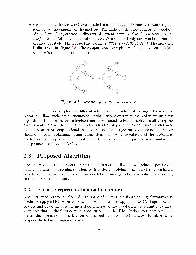
• Given an individual, or an O-tree encoded in a tuple (T, π), the mutation randomly re-permutates the sequence of the modules. The mutation does not change the topologyof the O-tree, but generates a di�erent placement. Suppose that (0011010001101,ad-bcegf) is an initial individual, and that abcdefg is the randomly generated sequence ofthe module labels. The mutated individual is (0011010001101,abcdefg). The mutationis illustrated in Figure 3.8. The computational complexity of this mutation is O(n),where n is the number of modules.
Figure 3.8: Initial O-tree (a) and the mutated O-tree (b)
In the previous examples, the di�erent solutions are encoded with strings. These repre-sentations allow e�cient implementations of the di�erent operators involved in evolutionaryalgorithms. In our case, the individuals must correspond to feasible solutions all along theexecution of the algorithm. This requires a validation step of the new solutions which trans-lates into an extra computational cost. Moreover, these representations are not suited forthermal-aware �oorplanning optimization. Hence, a new representation of the problem isneeded to e�ciently target our problem. In the next section we propose a thermal-aware�oorplanner based on the NSGA-II.
3.3 Proposed Algorithm
The designed genetic operators presented in this section allow us to produce a populationof thermal-aware �oorplaning solutions by iteratively applying these operators to an initialpopulation. The best individuals in the population converge to targeted solutions accordingto the metrics to be optimized.
3.3.1 Genetic representation and operators
A genetic representation of the design space of all possible �oorplanning alternatives isneeded to apply a MOEA correctly. Moreover, to be able to apply the NSGA-II optimizationprocess and cover all possible inter-dependencies of the topological constraints, we mustguarantee that all the chromosomes represent real and feasible solutions to the problem andensure that the search space is covered in a continuous and optimal way. To this end, wepropose the following representation:
28
• Every block i in the model Bi(i = 1, 2, . . . , n) is characterized by a width wi, a height hiand a length li while the design volume has a maximum widthW , maximum height H,and maximum length L. We de�ne the vector (xi, yi, zi) as the geometrical locationof block Bi, where 0 ≤ xi ≤ L − li, 0 ≤ yi ≤ W − wi, 0 ≤ zi ≤ L − hi. We use(xi, yi, zi) to denote the left-bottom-back coordinate of block Bi while we assume thatthe coordinate of left-bottom-back corner of the resultant IC is (0, 0, 0).
• we use a permutation encoding [9], where every chromosome is a string of labels, thatrepresents a position in a sequence.
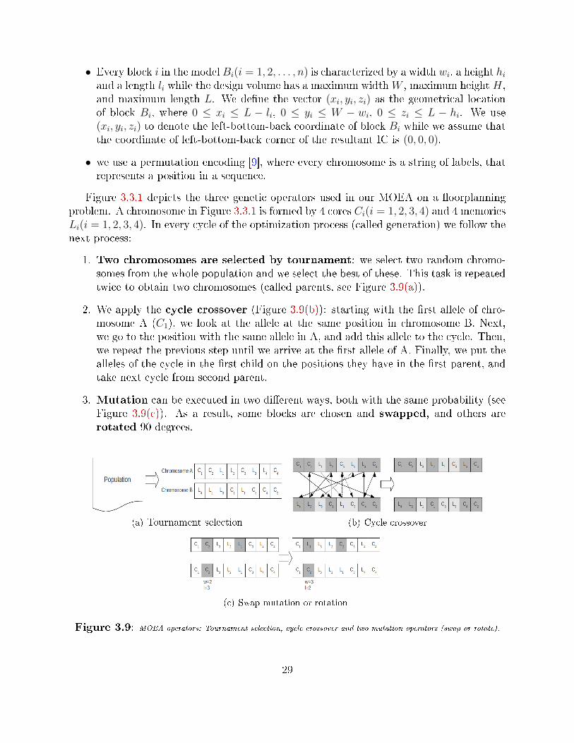
Figure 3.3.1 depicts the three genetic operators used in our MOEA on a �oorplanningproblem. A chromosome in Figure 3.3.1 is formed by 4 cores Ci(i = 1, 2, 3, 4) and 4 memoriesLi(i = 1, 2, 3, 4). In every cycle of the optimization process (called generation) we follow thenext process:
1. Two chromosomes are selected by tournament: we select two random chromo-somes from the whole population and we select the best of these. This task is repeatedtwice to obtain two chromosomes (called parents, see Figure 3.9(a)).
2. We apply the cycle crossover (Figure 3.9(b)): starting with the �rst allele of chro-mosome A (C1), we look at the allele at the same position in chromosome B. Next,we go to the position with the same allele in A, and add this allele to the cycle. Then,we repeat the previous step until we arrive at the �rst allele of A. Finally, we put thealleles of the cycle in the �rst child on the positions they have in the �rst parent, andtake next cycle from second parent.
3. Mutation can be executed in two di�erent ways, both with the same probability (seeFigure 3.9(c)). As a result, some blocks are chosen and swapped, and others arerotated 90 degrees.
(a) Tournament selection (b) Cycle crossover
(c) Swap mutation or rotation
Figure 3.9: MOEA operators: Tournament selection, cycle crossover and two mutation operators (swap or rotate).
29

3.3.2 Fitness function
Each chromosome represents the order in which blocks are being placed in the design area.Every block Bi is placed taking into account all the topological constraints, the total wirelength, and the maximum temperature in the chip with respect to all the previously placedblocks Bj : j < i. In order to place a block i, we take the best point (xi, yi, zi) in theremaining free positions. To select the best point we stablish a dominance relation takinginto account the m following objectives in our multi-objective evaluation:
• The �rst objective is determined by the topological relations among placed blocks.It represents the number of topological constraints violated (no overlapping betweenplaced blocks and current area less or equal than maximum area).
• The second objective is the wire length. The wire length is approximated as theManhattan distance between interconnected blocks.
• The following objectives (3, 4, . . . ,m) are a measures of the thermal impact, each onebased on a power consumption besed on our pro�les. In our case, we must obtain upto 600 di�erent power consumptions (100 time windows × 6 applications).
Obviously, 600 objectives is too high for a MOEA, since it is almost impossible toconverge. However, we discuss some ways to reduce this number of objectives in the nextchapter. The compute the thermal impact for every power consumption we cannot use anaccurate thermal model, which includes non-linear and di�erential equations. In a classicalthermal model, the temperature of a unitary cell of the chip, depends not only on the powerdensity dissipated by the cell, but also on the power density of its neighbors. The �rstfactor refers to the increase of the thermal energy due to the activity of the element, whilethe second one is related to the di�usion process of heat [28]. Taking this into account, weuse the power density of each block as an approximation of its temperature in the steadystate. This is a valid approximation because the main term of the temperature of a cell isgiven by the power dissipated in the cell, the contribution of its neighbors does not changesigni�cantly the thermal behavior. Thus, our remaining objectives can be formulated as:
Jk∈3..m =∑
i<j∈1..n
(dpk−2i ∗ dpk−2j )/(dij) (3.1)
where dppi is the power density of block i for power consumption p, and dij is the Euclideandistance between blocks i and j.
In the next chapter, we explain how we obtain the power pro�les for the di�erent scenariosand benchmarks. Later on, in Chapter 5 we present the di�erent parameters �xed to runthis algorithm and explain the experiments proposed in this work.
30

Chapter 4
Power Pro�ling Phase
In the �rst section we give a description of the chosen benchmarks and the changes done toadapt them to be run by the OVPsim simulator. In the second section we explain how theenergy pro�ling is carried out for the di�erent memories and processors considered.
4.1 Benchmarks
This work approaches the thermal-guided �oorplanning problem for manycore heteroge-neous architectures. The temperature of a given chip depends on physical factors such asthe power dissipation of the processors, the size of the memories etc. but it also dependson the dynamic pro�le of the applications. One of our contributions is to consider energypro�les based on the simulation of real world applications. In fact, this problem is generallyapproached considering only the worst case scenario in terms of power dissipation.
In this section we describe the benchmarks used and justify our choice. We work withParMiBench [23] (Open-Source Benchmark for Multiprocessor Based Embedded Systems)which is composed of parallel versions of typical applications. We select 11 applicationsgrouped into six di�erent categories: Calculus, Network, Security, O�ce, Multimedia andMixed. Therefore we have 6 di�erent benchmarks corresponding to di�erent kinds of appli-cations that will exhibit very di�erent execution pro�les. As a result the power dissipationpro�les obtained are di�erent from one benchmark to another. A brief description of eachof these benchmarks grouped into the di�erent categories can be found below.
• Calculus: The applications forming this category are mainly mathematical intensivecalculus applications such as solving cubic equations, converting values from deci-mal to radian, computing integer square roots, and bit counting in several di�erentways. In order to obtain representative energy pro�les, we choose the four followingapplications:
� a cubic equations solver
31

� a deg to rad conversion
� an integer square root
� a bitcount application
• Network: The applications forming this category are typical algorithms used in graphanalysis. In particular we choose a Dijkstra Shortest Path algorithm and a Patri-cia (Practical Algorithm to Retrieve Information Coded in Alphanumeric) algorithmworking with IP addresses. In order to obtain representative energy pro�les of networkapplications, we choose the two following applications:
� Dijkstra Shortest Path algorithm
� Patricia with IP addresses
• Security: The application forming this category implements a Secure Hash Algo-rithm (SHA), we consider only one benchmark for this category, enough to obtain arepresentative energy pro�le of security related applications.
� SHA
• O�ce: The applications forming this category perform a string search in a given inputtext with two di�erent methods. In order to obtain representative energy pro�les ofo�ce applications, we choose the two following applications:
� string search using the Boyer-Moore-Horspool method
� string search using the Pratt-Boyer-Moore method
• Multimedia: The applications forming this category are multimedia applicationsworking with images. These applications analyze the input image and produce a dif-ferent image as output. In order to obtain representative energy pro�les of multimediaapplications, we choose the two following applications:
� corner �nder
� image smoothing
• Mixed: We add an extra mixed pro�le that regroups two applications with a verydi�erent execution pro�le:
� Calculus applications
� Dijkstra shortest path algorithm
These applications are implemented with a shared memory strategy, in particular withPosix threads. This implementation is not the one we need to run the applications withOVPsim. It is due to the fact that we want to simulate these applications on bare machines(i.e. architectures that are not provided with an OS) to avoid the overhead caused by an
32

operating system in our power pro�les. Therefore the benchmarks need to be adapted tobe run by OVPsim (mapping the compiled code into speci�c memory regions, replacing thesystem calls etc.). The modi�cation of these applications is intuitive: we replace the codede�ning the POSIX threads with functions of the OVPsim Api. Hence the code executedby a POSIX thread in the original ParMiBench will now be executed by a processor de�nedin the architecture.
As we do not have any automatic tool to manage the use of shared memory, we mustassign manually a region to each of the executed programs. We also need to assign manu-ally a speci�c memory address to every variable declared as shared. For some programs ofthe benchmark, the size of the shared memory region needed depends on the input data.Hence, we are forced to �x these inputs and discover the amount of memory needed withpro�ling techniques. It is important to note that if the inputs were not �xed, memory re-gions addressed by di�erent processors could overlap. The accesses to the shared memory ofthe di�erent processors are always performed in a sequential way due to the multiprocessorscheduling algorithm used. Hence, we do not need to care about the integrity of the dataplaced in shared memory because, during the simulations, only one processor at a time willaccess this memory. It is important to note that some of these programs only need to useshared �ags while others need to share data, in some of them there is a lot of communicationwhile in others the processors are practically independent. Therefore the access patterns toshared memory and the processor state will be very di�erent from a given benchmark toanother.
To obtain the pro�ling statistics for a given benchmark and a given architecture, weproceed as follows :
1. we �x the amount of processors that will execute a given application
2. we �x which processors will work together
3. we assign a shared memory region to each of the groups of processors working together
We illustrate this idea with an example, we show the task distribution of the Networkbenchmark for the three considered architectures. The distribution for the rest of the sim-ulations is detailed in the Appendix A. With these task distributions, we aim to simulatescenarios that could happen on a real platform.
In the case of the 30 cores scenario (see Table 4.1), there are three groups of six processors(4 SPARC + 1 ARM + 1 PPC) computing the Dijkstra shortest path algorithm and 12processors (8 SPARC + 2 ARM + 2 PPC) computing a Patricia algorithm.
In the 66 cores scenario (see Table 4.2), we can see 7 groups of six processors (2 SPARC+ 2 ARM + 2 PPC) computing the Dijkstra shortest path algorithm and two groups of 12processors (4 SPARC + 4 ARM + 4 PPC) computing a Patricia algorithm.
Finally, in the 129 cores scenario (see Table 4.3), there are fourteen groups of six proces-sors (2 SPARC + 2 ARM + 2 PPC) computing the Dijkstra shortest path algorithm, three
33

Application SPARC id ARM id PPC id
Patricia 0,1,2,3,4,5,6,7 20,21 25,26
Dijkstra1 8,9,10,11 22 27
Dijkstra2 12,13,14,15 23 28
Dijkstra3 16,17,18,19 24 29
Table 4.1: Distribution of the Network benchmark for the 30 core architecture
Application SPARC id ARM id PPC id
Patricia1 0,1,2,3 22,23,24,25 44,45,46,47
Patricia2 4,5,6,7 26,27,28,29 48,49,50,51
Dijkstra1 8,9 30,31 52,53
Dijkstra2 10,11 32,33 54,55
Dijkstra3 12,13 34,35 56,57
Dijkstra4 14,15 36,37 58,59
Dijkstra5 16,17 38,39 60,61
Dijkstra6 18,19 40,41 62,63
Dijkstra7 20,21 42,43 64,65
Table 4.2: Distribution of the Network benchmark for the 66 core architecture
groups of 12 processors (4 SPARC + 4 ARM + 4 PPC) computing a Patricia algorithm anda group of 9 processors (3 SPARC + 3 ARM + 3 PPC) computing a Patricia algorithm.
4.2 Energy pro�les
We use some of the features provided by the OVPsim software to obtain these pro�les.As we showed in Chapter 2, the studied architectures are mainly composed of processorsand memories: a local memory for each of the processors and a common shared memory.The objective of this section is to compute the power dissipated by each of these elements.We perform simulations of the chosen benchmarks in the di�erent studied architectures.Therefore we need to obtain data from 3 * 6 = 18 simulations that provide us the statisticaldata we need to compute the power dissipated by each element. We study the evolution ofthe power dissipation over time for every element in the studied architecture. We proceedas follows:
1. We split the simulation of a given benchmark in time slices called windows
2. for each of these windows we obtain:
• for each processor:
� the amount of executed instructions
� the amount of idle cycles
34

Application SPARC id ARM id PPC id
Patricia1 0,1,2,3 43,44,45,46 86,87,88,89
Patricia2 4,5,6,7 47,48,49,50 90,91,92,93
Patricia3 8,9,10,11 51,52,53,54 94,95,96,97
Patricia4 12,13,14 55,56,57 98,99,100
Dijkstra1 15,16 58,59 101,102
Dijkstra2 17,18 60,61 103,104
Dijkstra3 19,20 62,63 105,106
Dijkstra4 21,22 64,65 107,108
Dijkstra5 23,24 66,67 109,110
Dijkstra6 25,26 68,69 111,112
Dijkstra7 27,28 70,71 113,114
Dijkstra8 29,30 72,73 115,116
Dijkstra9 31,33 74,75 117,118
Dijkstra10 33,34 76,77 119,120
Dijkstra11 35,36 78,79 121,122
Dijkstra12 37,38 80,81 123,124
Dijkstra13 39,40 82,83 125,126
Dijkstra14 41,43 84,85 127,128
Table 4.3: Distribution of the Network benchmark for the 129 core architecture
• for each memory (local and shared):
� the amount of read accesses
� the amount of write accesses
We obtain at least the statistical data of 100 windows. We �x the window period to 128ms.This value is chosen to be long enough to reduce the impact on performance of the pro�lingphase, but short enough to capture the dynamic behavior with the required accuracy. Thesimulations are at least 12.8s long (100× 0.128s), enough to reach a stationary state.
4.2.1 Memories
We assume that the energy consumption of the memories depends on the amount of read/writeaccesses. The energy consumption of the memories depends on di�erent factors such asmemory size, line size, associativity, transistor size, page size etc. We obtain the energyconsumption and area values with the CACTI software [20]. We approximate the energyper write access value with Ew = Er ∗ 1.5.
Local memories: The minimum size of the memories is found with pro�ling techniques.The application that needs the biggest amount of memory is the image smoothing wherethe studied image must be loaded into memory. If we limit the input images to small imageswe can run this application with 524288B ' 512KB of local memory (rounded up to the
35

nearest power of 2). As this applications is the worst case scenario, we �x the size of thelocal memories to 512KB.
We consider the local memories to be direct mapped SRAM memories, with a block sizeof 64 bytes and a transistor size of 45 nm. We obtain the following values:
• Total dynamic read energy per access: 0.584846 nJ
• Total dynamic write energy per access: 1,364895 nJ
• Area: 2.65952 mm2
Shared Memory: On the other hand, the size of the shared memory depends on thearchitecture we want to simulate. It is intuitive to think that a largest amount of processorswill need a largest memory space to communicate and share data. Once again pro�lingtechniques are used to �nd the minimum size of this memory in each of the three studiedarchitectures. We �x the memory sizes as follows (rounded up to the nearest power of 2):
• 4194304B ' 4MB for the 30 cores architecture
• 8388608B ' 8MB for the 66 cores architecture
• 16777216B ' 16MB for the 129 cores architecture
We consider the shared memories to be a direct mapped SRAM memories, with a blocksize of 64 bytes and a transistor size of 45 nm. We obtain the following values:
• 30 cores architecture:
� Total dynamic read energy per access: 2.37758 nJ
� Total dynamic write energy per access: 3,56637 nJ
� Area: 14.3553 mm2
• 66 cores architecture:
� Total dynamic read energy per access: 3.96696 nJ
� Total dynamic write energy per access: 5,95044 nJ
� Area: 28.256 mm2
• 129 cores architecture:
� Total dynamic read energy per access: 3.99656 nJ
� Total dynamic write energy per access: 5,99484 nJ
� Area: 57.513 mm2
36

4.2.2 Processors
We assume that the energy consumption of a given processor depends on its working fre-quency and its state. We consider two states: active or idle. To compute the power densitiesof the processors, we need their areas and a power consumption value for both the active andidle states. We approximate the power dissipated in the idle state with Pidle = Pactive/10.
• In [27] we �nd a power consumption of the sparc of 4W at 1.4GHz and an area of3.24mm2
• In the case of the cortex-A9[4], we �nd that 0.4W is the estimated power dissipationworking at 830 MHz with an area of 1.5mm2
• The ppc440 9SF[22] dissipates 1.1W at 667MHz and has an area of 6.2mm2
4.2.3 Power pro�les
Once we have the power consumption speci�cations of all the elements considered in thiswork, we need to obtain the dissipated power by each element in each time window.
In the case of the memories, it is immediate as we just need to multiply the di�erent ac-cesses counted during the simulations by the energy per access values retrieved with CACTI.
In the case of the processors, we proceed in a similar way. We need to compute theamount of active and idle cycles and multiply these values by the power consumption in theactive and idle states respectively.
The �oorplanner proposed in this work considers the power densities of the di�erentcomponents of our platforms. The power density of a given element i is computed with thefollowing formula:
dpi =pi
(lengthi ∗ cellsizeinµm ∗ 10−6 ∗ widthi ∗ cellsizeinµm ∗ 10−6)(4.1)
where pi is the power consumption, lengthi and widthi are the dimensions of the consideredelement and cellsizeinµm is the size of the cell used by the �oorplanner. The power densityof each element and time window are used to guide the �oorplanner as explained in the nextchapter (see 5.1).
To summarize this section, we show in Table 4.4 the areas and power consumption valuesof all the elements considered in this work.
37

area(mm2) l(mm) w(mm) en. r (nJ) en. w (nJ) p (W) freq(GHz)
SPARC 3.24 1.800 1.800 - - 4 1.4
Cortex-A9 1.5 1,225 1,225 - - 0.4 0.830
PPC440 6.2 2,490 2,490 - - 1.1 0.667
LMEM 2.660 1.129 2.357 0.584846 1,364895 - -
SMEM30 14.355 3.208 4.475 2.37758 3,56637 - -
SMEM66 28.256 3.155 8.957 3.96696 5,95044 - -
SMEM129 57.513 6.404 8.981 3.99656 5,99484 - -
Table 4.4: Energy consumption and sizes of the di�erent elements
38

Chapter 5
Experimental Work
5.1 Experimental Setup
The experimental work will analyze the thermal optimizations achieved by the �oorplannerin the three di�erent proposed scenarios in 2.3.3 (30, 66 and 129 cores architectures). The�oorplanner will place the processors, the local and shared memories of the 3D manycoreplatforms in 3, 4 and 5 layers respectively.
We compare four di�erent �oorplans obtained with our algorithm:
• As we do not have any original con�guration to compare with, we propose as baselinea performance optimized �oorplan targeting only the wire length. From now on, thiscon�guration will be called BAS.
In order to obtain the thermally optimized �oorplans, it is not possible to take directly intoaccount all the data retrieved from our simulations. In fact, if the power dissipation of everyelement for every benchmark and time window was considered, the �oorplanner would target600 objectives and would hardly converge. Therefore, to obtain the other three �oorplans,we consider di�erent power metrics computed with the data retrieved from the simulationof 100 time windows for the 6 di�erent execution pro�les.
• The �rst of the remaining con�gurations is obtained considering the mean powerdissipation for each element and pro�le (AVG). Therefore, the �oorplanner looks forfeasible solutions that minimize six thermal objectives (one per pro�le) and the wirelength.
• Another con�guration is obtained taking into account only the highest power con-sumption per element and pro�le (WOR). Hence, only two objectives are targeted, athermal objective and the wire length. This case corresponds to the strategy followedby other thermal-aware �oorplanners.
• Finally, a weighted sum of the power consumptions of the di�erent pro�les is consideredfor each element (WSM). In this case, the algorithm targets a thermal objective andthe wire length.
39

We run the multi-objective genetic algorithm with a population of 100 individuals and 500generations. These parameters are �xed according to previous research. The crossover prob-ability pc is �xed to 0.90 and the mutation probability pm to 1/#blocks (see [13]). We add20% of extra area to the di�erent layers to increase the e�cacy of the algorithm.
The con�gurations obtained are chosen among a front of non-dominated solutions re-turned by the �oorplanner. In the next section we explain how a solution of the non-dominated front is selected.
5.2 Results
As we explained in the previous section, the �oorplanner returns a set of non-dominatedsolutions. The di�erent solutions present in the returned front correspond to di�erent �oor-plans that have di�erent wire length and a di�erent thermal behaviour. We �rst analyze thewire length of the di�erent solutions obtained for the di�erent con�gurations and scenarios.The wire length is the sum of the Manhattan distances between the connected elements.The baseline (BAS) corresponds to a con�guration obtained targeting only the wire length.Therefore, it is an optimal con�guration in terms of performance. We compare the wirelength of the thermally optimized �oorplans to the baseline, this way we can evaluate thetradeo� between thermal optimization and performance. Table 5.1 shows the maximumand minimum wire length obtained for the di�erent solutions conforming a non-dominatedfront.
BAS AV G WOR WSMd dmin % dmax % dmin % dmax % dmin % dmax %
30 1700 2327 36.88 2964 74.35 2095 23.24 2328 36.94 1923.5 13.15 2034 19.6566 5643 6557 16.19 8639 53.09 7149 26.68 7949 40.87 6617 17.25 6794 20.40129 15178 18943 24.81 20996 38.33 17863 17.69 20558 35.45 18564 22.31 19208 26.55
Table 5.1: Wire overhead
We can see that in the case of the AVG con�guration, there is always a wide rangeof wire overhead. It is due to the fact that it is harder for the �oorplanner to convergewhen it targets a high number of objectives (seven objectives). On the other hand, thesolutions found for the WSM con�guration are more homogeneous which is an indicator ofthe convergence of the algorithm. The WOR case corresponds to an intermediate result interms of the convergence of the algorithm. These �rst results show that a relaxation ofthe thermal constraints (WSM) leads to a faster convergence of the �oorplanner.
We also observe that some of the solutions obtained are not acceptable. For example,in the case of the AVG con�guration for the 30 cores scenario, there is a wire overhead of74.35%. Such a con�guration implies a great loss of chip performance. To avoid such aperformance penalty and to easily select a solution among the returned front of solutions,we choose in each case the con�guration that presents the minimal wire overhead. Table5.2 shows the wire overhead of the selected solutions. We can see that in each of the three
40

scenarios (30, 66 and 129 cores), the best wire overhead is found for a di�erent con�guration.In fact, the WSM con�guration is the most e�cient con�guration for the 30 cores scenario,AVG outperforms the others in the 66 processors case while in the last scenario, the bestperformance is obtained by the WOR con�guration.
BAS AV G WOR WSMDist % Dist % Dist % Dist %
30 1700 0.00 2327 36.88 2095 23.24 1923.5 13.1566 5643 0.00 6557 16.19 7149 26.68 6617 17.25129 15178 0.00 18943 24.81 17863 17.69 18564 22.31
Table 5.2: Wire Overhead
As further analysis will show, solutions with a reduced wire length tend to have a poorthermal behaviour. On the other hand, the higher the wire length, the better the thermalresponse of a given solution. In this section, we compare the thermal pro�les of the di�erentcon�gurations obtained in 5.1 and propose a way to deal with the performance/temperaturetradeo�. We propose two experiments, in the �rst one we evaluate the thermal responseof the di�erent con�gurations in the worst case scenario. In the second experiment, thethermal behaviour of these con�gurations is studied with the real power pro�les retrievedfrom our simulations.
5.2.1 Worst Case Scenario
In the �rst experiment, the thermal simulator evaluates the di�erent �oorplans with thehighest power dissipation for every element. This case corresponds to the worst scenario.The metrics considered for the analysis of the experimental results are the mean and maxi-mum temperature of the chip and the maximum thermal gradient. These metrics are usuallyfound in thermal-related analysis. In table 5.3, 5.4 and 5.5 we present the thermal pro�lesof the four di�erent con�gurations.
WireOverhead Tmax Tmean GradMax
BAS 0% 416.30 355.22 108.44
AVG 36.88% 394.80 350.10 84.93
WOR 23.24% 388.42 349.03 73.46
WSM 13.15% 387.68 349.73 74.12
Table 5.3: Worst case 30 cores
The results show that our power pro�ling-guided �oorplanner produces thermally opti-mized con�gurations. The hotspots found in the performance optimized �oorplansjustify the thermal optimization presented in this work. Compared to the baseline,we can see that in all the cases our �oorplanner reduces the peak and mean temperaturesand the thermal gradient. Therefore, not only the temperature of the chip is reduced but it
41

WireOverhead Tmax Tmean GradMax
BAS 0% 440.24 357.35 136.10
AVG 16.19% 410.187 352.41 101.92
WOR 26.68% 401.27 349.55 91.22
WSM 17.25% 403.34 349.40 91.742
Table 5.4: Worst case 66 cores
WireOverhead Tmax Tmean GradMax
BAS 0% 443.15 361.56 137.57
AVG 24.81% 396.33 355.32 87.06
WOR 17.69% 414.45 355.98 104.59
WSM 22.31% 400.44 354.63 91.75
Table 5.5: Worst case 129 cores
is more evenly distributed. For example, we can appreciate that the dramatic peak tempera-ture of 416.30K found in the baseline is reduced to 387.68K in the WSM con�guration in the30 core platform. We illustrate this example in Figure 5.1 where we show the thermal mapsof the �rst layer of the BAS and WSM con�gurations. In the baseline con�guration the�oorplanner tends to place the processors near their local memories ignoring the presenceof hotspots. In the other the hottest elements (the SPARC cores) are separated as much aspossible, generally placed in the borders of the chip. As a consequence, we observe a muchbetter thermal response of the WSM con�guration. Vertical heat spread is also taken intoaccount, hence the �oorplanner avoids placing cores above the others. In both cases theshared memory is placed in the second layer to minimize the wire length.
Figure 5.1: Thermal map of the �rst layer of the 30 cores BAS(left) and WSM(right) con�gura-
tions
42

The baseline con�guration (BAS) is not an acceptable solution, in fact it reaches peaksof 443.15K in the 129 cores con�guration. Moreover, the peak temperature increases withthe number of cores in all of the cases. Therefore, from now on we will use the baselineto compare the wire length of the thermally optimized �oorplans, but we will not study itsthermal response.
Choosing a con�guration between the thermally optimized �oorplans is not immediate.It is due to the fact that some of these con�gurations present a better performance (wirelength) while others have a better thermal behaviour. We propose a selection criterion in5.2.3.
5.2.2 Real power Pro�les
In the second experiment proposed, we evaluate the �oorplans in a more realistic way, thethermal behaviour of the di�erent con�gurations is simulated for 100 time windows with thepower dissipation values obtained from our execution pro�les. Three metrics are consideredin this case to compare the di�erent con�gurations:
• The mean of the maximum temperatures of the di�erent time windows is given as wellas its standard deviation. This metric is a good indicator of the existence of hotspotsin the studied chip.
• We also compute the overall mean temperature of the chip and its standard deviation.
• The mean of the maximum thermal gradients and its standard deviation is presentedas well.
In Table 5.6 (30 cores scenario), Table 5.7 (66 cores scenario) and Table 5.8 (129 coresscenario) we present these metrics for the six studied benchmarks and the three di�erentcon�gurations.
Table 5.6: 30 cores architectureWire Tmax
BENCH1 BENCH2 BENCH3 BENCH4 BENCH5 BENCH6
AVG 36.88% 340.956.58 342.554.56 340.227.80 310.353.15 348.332.68 343.753.38WOR 23.24% 338.737.44 345.512.66 341.1211.09 311.432.82 347.482.60 340.293.22WSM 13.15% 335.936.30 345.563.79 340.8010.02 309.372.89 346.652.56 341.382.63
Wire Tmean
BENCH1 BENCH2 BENCH3 BENCH4 BENCH5 BENCH6
AVG 36.88% 322.436.14 320.112.26 324.705.59 306.281.95 331.411.65 325.562.86WOR 23.24% 322.195.79 319.822.19 324.335.49 306.241.91 330.291.58 324.802.70WSM 13.15% 322.506.07 319.962.36 324.645.65 306.211.98 331.371.64 325.492.95
Wire Tgrad
BENCH1 BENCH2 BENCH3 BENCH4 BENCH5 BENCH6
AVG 36.88% 35.885.83 39.454.58 34.406.32 8.472.63 42.702.43 38.733.60WOR 23.24% 31.856.25 40.662.65 32.257.97 9.541.95 36.522.08 31.574.45WSM 13.15% 29.364.44 41.993.99 34.058.39 7.032.24 36.592.10 34.182.83
43

30 cores scenario: The results obtained for the peak temperatures are not conclusiveas none of the con�gurations clearly outperforms the others. The highest di�erence isobtained in the case of the �rst Benchmark where the temperature reached by the WSMis 2.8oC and 5.02oC lower than the one obtained with the WOR and AVG con�gurationsrespectively. The mean temperatures are very similar for all the con�gurations. In factthere is a maximum di�erence of 1.12oC between the di�erent con�gurations (Benchmark5). As for the peak temperatures, a �rst analysis of the maximum thermal gradients doesnot lead to an immediate selection of the best con�guration. Further analysis of these resultsis proposed in 5.2.3 where we �nd the con�guration that minimizes wire length and thermalmetrics for each benchmark.
Table 5.7: 66 cores architectureWire Tmax
BENCH1 BENCH2 BENCH3 BENCH4 BENCH5 BENCH6
AVG 16.19% 334.179.35 365.437.36 386.493.14 369.641.64 349.523.12 369.164.64WOR 26.68% 329.775.60 366.916.16 385.905.75 369.601.94 342.912.63 368.725.68WSM 17.25% 331.406.28 364.667.52 383.271.96 369.331.62 342.302.62 367.965.62
Wire Tmean
BENCH1 BENCH2 BENCH3 BENCH4 BENCH5 BENCH6
AVG 16.19% 319.615.22 325.631.06 338.793.43 324.900.60 328.271.51 324.630.62WOR 26.68% 318.364.16 325.910.92 337.963.81 324.770.54 325.231.36 324.510.71WSM 17.25% 318.574.40 325.270.96 337.293.18 324.330.55 325.401.36 323.830.65
Wire Tgrad
BENCH1 BENCH2 BENCH3 BENCH4 BENCH5 BENCH6
AVG 16.19% 29.508.42 62.357.65 80.752.22 66.991.87 44.483.04 66.254.98WOR 26.68% 24.753.95 64.356.60 79.995.51 67.352.24 35.352.56 66.426.43WSM 17.25% 26.024.93 61.417.94 76.901.23 66.912.02 34.432.38 65.456.59
66 cores scenario: We can see that the peak temperatures obtained in the WSM arelower than those obtained in the AVG con�guration saving up to 7.22oC. Only in the caseof the Benchmark 1 the peak temperature of the WOR con�guration is the lowest one,with a di�erence of 1.63oC over the WSM. On the other hand, selecting WSM leads to amaximum reduction of 2.63oC in the peak temperature for the Benchmark 3. Once again,there are no signi�cant di�erences between the mean temperatures obtained for the studiedcon�gurations. In the case of the maximum thermal gradients, the results are similar tothose obtained for the peak temperature: the WSM outperforms the other con�gurationsin �ve out of six cases, reducing up to 10.05oC the gradient of the AVG (Benchmark 5) and3.09oC the gradient of the WOR (Benchmark 3). In the case of the Benchmark 1, the bestthermal gradient is obtained for the WOR con�guration, with a di�erence of 1.27oC and4.75oC with the WSM and AVG con�gurations respectively.
129 cores scenario: The best peak temperature is obtained for the AVG con�gurationin four out of six benchmarks saving up to 17.12oC and 6.71oC comparing with the WOR(Bench 5) and WSM (Bench 1) con�gurations respectively. The WSM outperforms theothers in the remaining two cases, reducing up to 10.80oC the maximum temperature ofthe WOR con�guration and 2.98oC the one of the AVG. The mean temperatures obtained
44

Table 5.8: 129 cores architectureWire Tmax
BENCH1 BENCH2 BENCH3 BENCH4 BENCH5 BENCH6
AVG 24.81% 342.317.94 357.950.78 373.184.97 352.951.50 370.424.13 331.632.46WOR 17.69% 354.088.90 363.765.07 382.009.27 352.402.51 387.545.19 338.282.93WSM 22.31% 349.024.73 363.990.87 371.204.10 351.141.54 373.874.34 336.102.68
Wire Tmean
BENCH1 BENCH2 BENCH3 BENCH4 BENCH5 BENCH6
AVG 24.81% 327.325.80 328.681.34 338.784.53 321.701.86 344.242.36 322.201.57WOR 17.69% 328.255.95 329.191.49 339.014.77 321.571.89 344.872.40 322.571.61WSM 22.31% 327.995.52 328.521.43 338.204.99 320.561.98 344.122.35 322.551.59
Wire Tgrad
BENCH1 BENCH2 BENCH3 BENCH4 BENCH5 BENCH6
AVG 24.81% 36.086.31 54.771.00 66.813.52 51.021.07 62.043.77 25.862.14WOR 17.69% 47.757.79 60.064.79 75.958.28 50.701.97 78.824.80 32.122.56WSM 22.31% 43.713.80 61.040.91 65.843.22 49.451.14 66.283.98 31.902.49
are again homogeneous. The results for the the thermal gradients are similar to the onesobtained for the peak temperature. Globally, the WOR con�guration shows a worst thermalbehavior than the WSM or AVG. Nonetheless, it is the con�guration that presents the bestperformance (wire overhead), therefore it can not be discarded.
Further analysis is required in all the scenarios studied to obtain the optimum con�g-uration. In the next section we propose a method to select the optimum solution for thethree scenarios taking into account the wire length and the thermal behavior of the di�erentcon�gurations.
5.2.3 Performace/temperature tradeo�
As seen in the previous subsection, there is a tradeo� between performance and chip tem-perature. We propose a method to evaluate the di�erent solutions and select the one withthe best overall behaviour. For each of the scenarios and metrics studied (wire, TMax, Tmean
and GradMax) we establish a con�dence interval. In a second step we see wether or not theretrieved metrics fall into these ranges of acceptable values.
The con�dence intervals are obtained by adding and subtracting a given percentage tothe mean of the metric considered. This percentage is di�erent for each metric, as the rangesof the values obtained are very di�erent from a metric to another. We �x a percentage of:
• TMax and TMean metrics: we �x a percentage of 1%, this parameter results in con�denceintervals of approximately 6oC
• GradMax metric: we �x a percentage of 5% also resulting in con�dence intervals ofapproximately 6oC
• Wire overhead metric: we �x a percentage of 10% resulting in con�dence intervals ofapproximately 4 units (percentage relative to the wire overhead comparing with thebaseline con�guration)
As an example, we compute these intervals for the worst case scenario:
45

• 30 cores architecture
� Wire overhead: we obtain the mean of the wire overhead of the di�erent con-�gurations, which is 24.42%. The con�dence interval is obtained by adding andsubtracting a 10%, the resultant interval is :mean = 24.42%→ [24.42− 10%; 24.42 + 10%] ' [21.98; 26.86]
� TMax: in a similar way, we obtain the range of acceptable peak temperatures byadding and subtracting 1% of the mean of the maximum temperatures of thedi�erent con�gurations:mean = 390.2→ [390.2− 1%; 390.2 + 1%] ' [386.30; 394.10]
� Tmean: The same method is used to obtain the con�dence interval for the meantemperatures:mean = 349.62→ [349.62− 1%; 349.62 + 1%] ' [346.12; 353.12]
� GradMax: the range of acceptable values for the maximum thermal gradient isobtained by adding and subtracting 5% to the mean of the maximum thermalgradients(77.5K) of the di�erent �oorplans.mean = 77.5→ [77.5− 5%; 77.5 + 5%] ' [73.63; 81.375]
The same method is used for the 66 and 129 cores scenarios. We show the mean of theconsidered metric and the corresponding con�dence interval:
• 66 cores architecture:
� Wire overhead: mean = 20.04%→ [18.04; 22.04]
� TMax: mean = 404.93→ [404.93− 1%; 404.93 + 1%]
� Tmean: mean = 350.45→ [350.45− 1%; 350.45 + 1%]
� GradMax: mean = 94.96→ [94.96− 5%; 94.96 + 5%]
• 129 cores architecture
� Wire overhead: mean = 21.60%→ [19.44; 23.76]
� TMax: mean = 403.74→ [403.74− 1%; 403.74 + 1%]
� Tmean: mean = 355.31→ [355.31− 1%; 355.31 + 1%]
� GradMax: mean = 94.47→ [94.47− 5%; 94.47 + 5%]
These intervals allow us to put into the same level similar values, in fact a di�erenceof 1oC might not relevant to decide which con�guration is better. On the other hand,stepping from a 15% of area overhead to 25% would result in a dramatic decrease of thechip performance.
Once we have these intervals, we see which metrics fall into these intervals (marked as√in the following tables) and which ones do not (X). There is a third possibility where
the metric considered is even below the con�dence interval(marked as√√
), which is the
46

desirable situation as the goal is to minimize the wire length and the di�erent thermalmetrics. The following tables show the result of this analysis for the worst case scenario andthe 6 benchmarks. We perform an analysis based on the obtained con�dence intervals anddecide which is the best con�guration for each of the considered cases.
Worst Case
Table 5.9 shows the results of the analysis based on the con�dence intervals in the worst casescenario. This case corresponds to the highest power dissipation possible for the studiedchips. Hence it is representative of the chip response in extreme conditions.
30 Wire Tmax Tmean GradMax
AVG X X√
XWOR
√ √ √ √√
WSM√√ √ √ √
66 Wire Tmax Tmean GradMax
AVG√√
X√
XWOR X
√ √ √
WSM√√ √ √ √
129 Wire Tmax Tmean GradMax
AVG X√√ √ √√
WOR√√
X√
XWSM
√ √ √ √
Table 5.9: Worst case
30 cores scenario: We can see that only the WOR and the WSM con�gurations satisfyall the constraints. The WSM has 10.09% less of of wire overhead and thus, presents agreater performance. On the other hand, the WOR con�guration presents a better thermalgradient, reducing in 2.61oC the gradient of the WSM. Therefore, both the WSM and WORcon�gurations are chosen in this case.
66 cores scenario: In this case, the WSM is the only con�guration with acceptablevalues for all the metrics. Hence it is the selected con�guration.
129 cores: In this case, the WSM is also the only con�guration that satis�es all theconstraints, therefore we select the WSM.
Figure 5.2: Selected con�gurations in the Worst Case
47

Benchmark 1
Table 5.10 shows the results of the analysis based on the con�dence intervals obtained forthe Benchmark 1. This case corresponds to the power dissipation of the studied chips whileexecuting the MATH benchmark.
30 Wire Tmax Tmean GradMax
AVG X√ √
XWOR
√ √ √ √
WSM√√ √ √ √√
66 Wire Tmax Tmean GradMax
AVG√√ √ √
XWOR X
√ √ √
WSM√√ √ √ √
129 Wire Tmax Tmean GradMax
AVG X√√ √ √√
WOR√√
X√
XWSM
√ √ √ √
Table 5.10: BENCHMARK1
30 cores scenario: We can see that the WOR and the WSM con�gurations correspondto acceptable solutions. Nevertheless WSM presents a better performance and thermalgradient. Therefore, WSM is the best con�guration.
66 cores scenario: In this case, the WSM is the only con�guration with accepatablevalues for all the metrics. Hence it is the selected con�guration.
129 cores: The WSM is also the only con�guration that satis�es all the constraints,therefore we select the WSM.
Figure 5.3: Selected con�gurations for the Bench 1
48
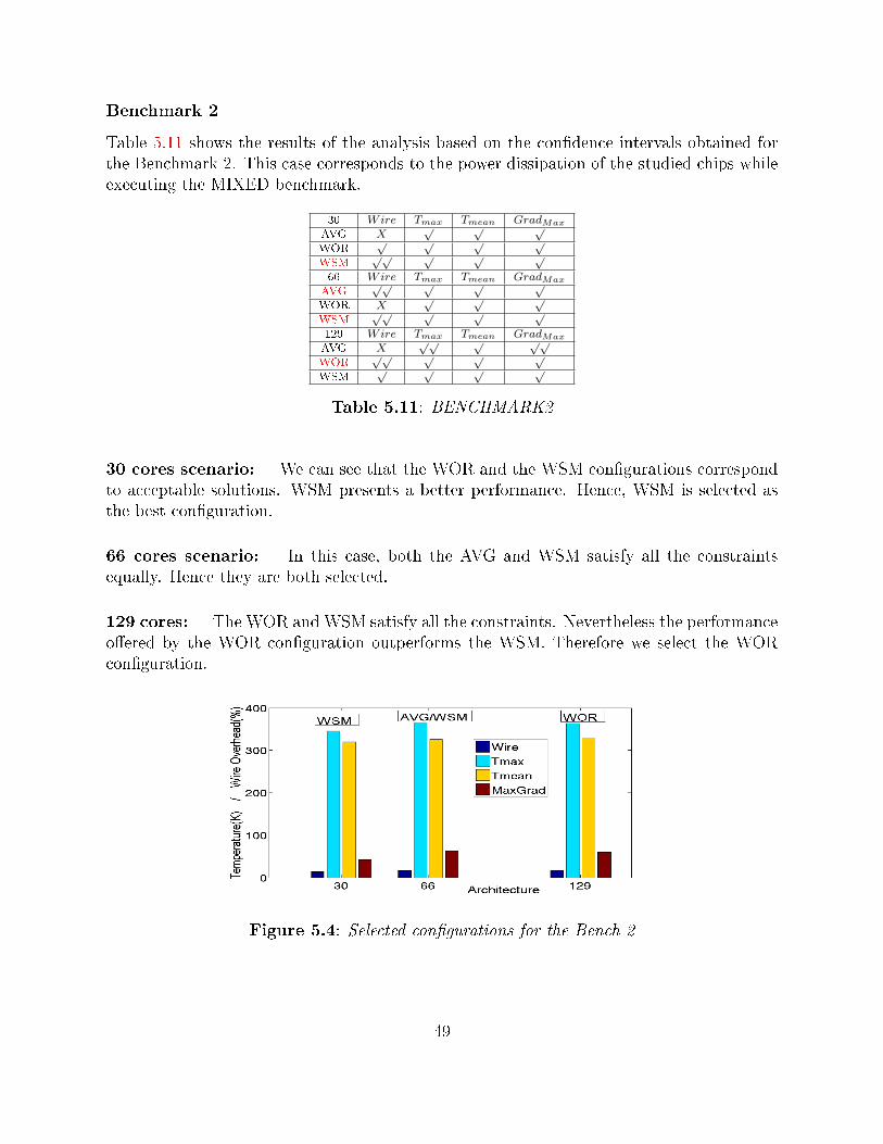
Benchmark 2
Table 5.11 shows the results of the analysis based on the con�dence intervals obtained forthe Benchmark 2. This case corresponds to the power dissipation of the studied chips whileexecuting the MIXED benchmark.
30 Wire Tmax Tmean GradMax
AVG X√ √ √
WOR√ √ √ √
WSM√√ √ √ √
66 Wire Tmax Tmean GradMax
AVG√√ √ √ √
WOR X√ √ √
WSM√√ √ √ √
129 Wire Tmax Tmean GradMax
AVG X√√ √ √√
WOR√√ √ √ √
WSM√ √ √ √
Table 5.11: BENCHMARK2
30 cores scenario: We can see that the WOR and the WSM con�gurations correspondto acceptable solutions. WSM presents a better performance. Hence, WSM is selected asthe best con�guration.
66 cores scenario: In this case, both the AVG and WSM satisfy all the constraintsequally. Hence they are both selected.
129 cores: The WOR and WSM satisfy all the constraints. Nevertheless the performanceo�ered by the WOR con�guration outperforms the WSM. Therefore we select the WORcon�guration.
Figure 5.4: Selected con�gurations for the Bench 2
49
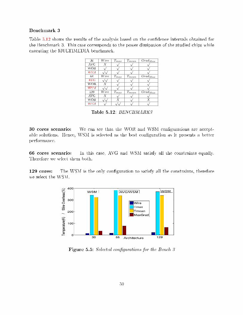
Benchmark 3
Table 5.12 shows the results of the analysis based on the con�dence intervals obtained forthe Benchmark 3. This case corresponds to the power dissipation of the studied chips whileexecuting the MULTIMEDIA benchmark.
30 Wire Tmax Tmean GradMax
AVG X√ √ √
WOR√ √ √ √
WSM√√ √ √ √
66 Wire Tmax Tmean GradMax
AVG√√ √ √ √
WOR X√ √ √
WSM√√ √ √ √
129 Wire Tmax Tmean GradMax
AVG X√ √ √
WOR√√
X√
XWSM
√ √√ √ √
Table 5.12: BENCHMARK3
30 cores scenario: We can see that the WOR and WSM con�gurations are accept-able solutions. Hence, WSM is selected as the best con�guration as it presents a betterperformance.
66 cores scenario: In this case, AVG and WSM satisfy all the constraints equally.Therefore we select them both.
129 cores: The WSM is the only con�guration to satisfy all the constraints, thereforewe select the WSM.
Figure 5.5: Selected con�gurations for the Bench 3
50

Benchmark 4
Table 5.13 shows the results of the analysis based on the con�dence intervals obtained forthe Benchmark 4. This case corresponds to the power dissipation of the studied chips whileexecuting the NETWORK benchmark.
30 Wire Tmax Tmean GradMax
AVG X√ √ √
WOR√ √ √
XWSM
√√ √ √ √√
66 Wire Tmax Tmean GradMax
AVG√√ √ √ √
WOR X√ √ √
WSM√√ √ √ √
129 Wire Tmax Tmean GradMax
AVG X√ √ √
WOR√√ √ √ √
WSM√ √ √ √
Table 5.13: BENCHMARK4
30 cores scenario: The WSM is the only con�guration that satis�es all the constraints,therefore it is selected.
66 cores scenario: AVG and WSM satisfy all the constraints equally. Therefore weselect both of them as best con�gurations.
129 cores: We can see that WOR and WSM con�gurations correspond to acceptablesolutions. WOR is selected as it presents a better performance.
Figure 5.6: Selected con�gurations for the Bench 4
51

Benchmark 5
Table 5.14 shows the results of the analysis based on the con�dence intervals obtained forthe Benchmark 5. This case corresponds to the power dissipation of the studied chips whileexecuting the OFFICE benchmark.
30 Wire Tmax Tmean GradMax
AVG X√ √
XWOR
√ √ √ √√
WSM√√ √ √ √√
66 Wire Tmax Tmean GradMax
AVG√√
X√
XWOR X
√ √ √√
WSM√√ √ √ √√
129 Wire Tmax Tmean GradMax
AVG X√√ √ √√
WOR√√
X√
XWSM
√ √ √ √
Table 5.14: BENCHMARK5
30 cores scenario: We can see that WOR and WSM con�gurations correspond toacceptable solutions. WSM is selected as it presents a better performance.
66 cores scenario: The WSM is the only con�guration that satis�es all the constraints.Hence, it is selected.
129 cores: The WSM is the only acceptable con�guration. Therefore we select WSM asthe best con�guration.
Figure 5.7: Selected con�gurations for the Bench 5
52

Benchmark 6
Table 5.15 shows the results of the analysis based on the con�dence intervals obtained forthe Benchmark 6. This case corresponds to the power dissipation of the studied chips whileexecuting the SECURITY benchmark.
30 Wire Tmax Tmean GradMax
AVG X√ √
XWOR
√ √ √ √√
WSM√√ √ √ √
66 Wire Tmax Tmean GradMax
AVG√√ √ √ √
WOR X√ √ √
WSM√√ √ √ √
129 Wire Tmax Tmean GradMax
AVG X√√ √ √√
WOR√√ √ √
XWSM
√ √ √X
Table 5.15: BENCHMARK6
30 cores scenario: We can see that only the WOR and the WSM con�gurations satisfyall the constraints. The WSM has presents a better performance. On the other hand,the WOR con�guration presents a better thermal gradient. Therefore, both the WSM andWOR con�gurations are chosen in this case.
66 cores scenario: The AVG and WSM con�gurations satisfy all the constraints equally.Therefore we select both of them.
129 cores: In this case, none of the con�gurations satis�es all the constraints. Never-theless the WOR and WSM do not satisfy the thermal gradient constraint, i.e. they fall outof the interval by 0.66oC and 0.44oC respectively which is not signi�cant. Moreover, theirpeak temperatures reached in this benchmark are low: 338.28K for the WOR and 336.10Kfor the WSM con�gurations. Therefore, we choose a solution between the WOR and WSMsolutions. WOR presents a better performance, therefore it is selected.
Figure 5.8: Selected con�gurations for the Bench 6
53

5.2.4 Results summary
In this section we summarize the results of the experiments proposed in the previous sections.Figure 5.9 shows the con�gurations chosen for the di�erent benchmarks and scenarios. Weanalyze the con�guration with the best overall behavior in each scenario.
30 cores scenario: In this scenario only the WSM con�guration is chosen for all thebenchmarks. It o�ers a satisfactory performance while respecting the di�erent thermalmetrics studied in this work. The WOR con�guration is also selected in two out of 7 cases(Worst Case and Bench 6). Moreover, this con�gurations respects the di�erent constraintsin all the studied cases. However the WSM o�ers a better performance as it presents 10.09%less of wire overhead. Therefore the WSM is the best con�guration for the 30 coresscenario.
66 cores scenario: The WSM con�guration is also chosen in all the cases. It presentsthe best overall thermal behavior while only the AVG presents a slightly better performance(1.06%). The AVG con�guration presents the best performance and is also chosen in four outof seven cases but it does not satisfy the thermal constraints in the Worst and Benchmark 5cases. Therefore it o�ers a poor response in extreme situations, leading to hotspots. Hencethe WSM is also chosen in this scenario as the best con�guration.
129 cores: The selection of the best con�guration is not immediate as in the previousscenarios. In fact, the WOR con�guration is chosen in three out of seven cases (Benchmarks2, 4 and 6) that correspond to the MIXED, NETWORK and SECURITY benchmarks.These data-oriented benchmarks are not loop-dominated, in fact they are executed in asequential manner presenting an elevated number of branch instructions. In addition, powerconsumption is distributed in an homogeneous way during the execution of these kind ofapplications which makes the Worst Case approximate well the dissipated power in thesecases. Nevertheless this con�guration violates the peak temperature and thermal gradientconstraints in four of the seven studied cases (Worst, Benchmarks 1,3,5). On the otherhand the WSM con�guration is chosen in four out of seven cases and presents acceptablesolutions in all the cases except for Benchmark 6, where none of the con�gurations respectsall the constraints. In that particular case, the analysis shows that it fails to minimize thethermal gradient by 0.44oC and the peak temperature reached is not critical (331.6K '63.1oC), therefore the solution remains acceptable. Hence, the WSM is the con�gurationthat presents best overall behavior. The WSM con�guration is also chosen in thisscenario.
54

(a) WORST CASE (b) Benchmark 1
(c) Benchmark 2 (d) Benchmark 3
(e) Benchmark 4 (f) Benchmark 5
(g) Benchmark 6
Figure 5.9: Best Con�guration for each Benchmark
55

Chapter 6
Conclusions and Future Work
In this work we propose for a �rst time a scalable e�cient thermal-aware 3D �oorplannerfor heterogeneous architectures of MPSoCs that uses as input the power traces obtainedduring an application power pro�ling phase.
The power pro�les are retrieved from simulations of manycore heterogeneous architec-tures and correspond to the dynamic pro�les of di�erent real world applications. Thesesimulations are carried out with the multiprocessor platform emulator OVPsim.
We design three manycore heterogeneous architectures inspired in Intel's Single-ChipCloud Computer. The designed heterogeneous platforms are composed of SPARC cores andthe low power oriented processors ARM Cortex-A9 and PPC440 9SF. Our architectures arecomposed of 30, 66 and 129 cores with their local memories and a common shared memoryused for inter-processor communication. Such manycore heterogeneous architectures areexpected to be the future trend in computer design.
The ParMiBench suite is adapted to be run on bare machines and simulated with OVP-sim to avoid the power overhead caused by an operating system. This suite contains severalCalculus, Network, Security, O�ce and Multimedia applications that exhibit very di�erentexecution pro�les.
We propose a scalable Multi-Objective Genetic Algorithm based on the NSGA-II capa-ble of proposing �oorplans for our architectures composed of 30, 66 and 129 cores. Previousresearch shows that MILP based techniques are unable to propose solutions in the lattercase. We propose a representation of the solutions and genetic operators that lead to opti-mal �oorplans, in a short time, for a large number of integrated processors and layers andwith minimal overhead.
The proposed multi-objective genetic algorithm returns di�erent �oorplans by targetingup to six di�erent thermal objectives and the wire length. We evaluate these con�gurationswith real power values retrieved from the simulation of 6 di�erent benchmarks.
56

The proposed analysis of the tradeo� between thermal behavior and performance showsthat considering the worst power consumption does not lead to optimal �oorplans. In fact,when we take into account performance and thermal metrics, a �oorplan that tries to mini-mize the weighted sum of the power consumption of the di�erent benchmarks shows a betteroverall behavior. Such con�guration presents a better thermal response in extreme condi-tions and reduces in 13,67oC and 12,54oC the peak temperature and the thermal gradientof the chip respectively. Therefore, the e�ect of hotspots is reduced and the temperature ofthe chip is more evenly distributed.
We show that considering the worst case in terms of power consumption leads to nonoptimal �oorplans due to an overestimation of the temperature of the chip. Therefore, apower pro�ling phase of representative applications that will run in the considered architec-tures is necessary to �nd thermally optimized solutions.
We have found a metric (WSM) that is able to outperform the results of the traditionallyused WOR (Worst case) for a set of representative benchmarks of the application scope.
The choice of the optimum �oorplan among the set of non-dominated solutions returnedby the �oorplanner is postponed as a future work.
Future research also expects to �nd a lower number of meaningful windows to reducethe overhead of pro�ling.
Finally, a better representation of the thermal-aware �oorplanning problem or a parallelversion of the genetic algorithm could increase the e�ciency of our algorithm. These im-provements would allow to study the convergence of the algorithm with an increase in thenumber of cores. This is a promising study as computer designers tend to place more andmore cores in a single die which makes existing thermal hotspots more severe.
57

Bibliography
[1] Electrothermal monte carlo modelling of submicron hfets.www.nanofolio.org/research/paper03.php, 2004.
[2] Intel tries to keep it cool.www.pcworld.idg.com.au/article/108386/intel tries keep its cool, 2004.
[3] S.N. Adya et al. Fixed-outline �oorplanning: enabling hierarchical design. VLSI Sys-tems, IEEE Transactions on, 11(6):1120 � 1135, dec. 2003.
[4] ARM. www.arm.com/products/processors/cortex-a/cortex-a9.php.
[5] Johan Berntsson and Maolin Tang. A slicing structure representation for the multi-layer�oorplan layout problem. In EvoWorkshops, pages 188�197, 2004.
[6] S. Borkar. Design challenges of technology scaling. Micro, IEEE, 19(4), 1999.
[7] G. Chen et al. Partition-driven standard cell thermal placement, 2003.
[8] C. Chu et al. A matrix synthesis approach to thermal placement. CADICS, IEEETransactions on, 17(11):1166 �1174, nov 1998.
[9] C. Coello et al. Evolutionary Algorithms for Solving Multi-Objective Problems. Kluwer,2002.
[10] Carlos A. Coello Coello. A short tutorial on evolutionary multiobjective optimization.In Proceedings of the First International Conference on Evolutionary Multi-CriterionOptimization, EMO '01, pages 21�40, London, UK, 2001. Springer-Verlag.
[11] J. Cong et al. A thermal-driven �oorplanning algorithm for 3D ICs. ICCAD, 2004.
[12] Jose L. Ayala David Cuesta, Jose L. Risco and D. Atienza. 3d thermal-aware �oorplan-ner for many-core single-chip systems. IEEE Latin-American Test Workshop, 2011.
[13] K. Deb et al. A fast and elitist multiobjective genetic algorithm: NSGA-II. IEEETransactions on Evolutionary Computation, 6(2):182�197, 2002.
[14] M. Ekpanyapong et al. Thermal-aware 3d microarchitectural �oorplanning. Technicalreport, Georgia Institute of Technology Center, 2004.
[15] Carlos M. Fonseca and Peter J. Fleming. Genetic Algorithms for Multiobjective Opti-mization: Formulation, Discussion and Generalization. In Genetic Algorithms: Proceed-ings of the Fifth International Conference, pages 416�423. Morgan Kaufmann, 1993.
58

[16] Pei-Ning Guo, T. Takahashi, Chung-Kuan Cheng, and T. Yoshimura. Floorplanningusing a tree representation. Computer-Aided Design of Integrated Circuits and Systems,IEEE Transactions on, 20(2):281 �289, feb 2001.
[17] I. K. Y. Han et al. Temperature aware �oorplanning, 2005.
[18] Y. Han et al. Simulated annealing based temperature aware �oorplanning, 2007.
[19] M. Healy et al. Multiobjective microarchitectural �oorplanning for 2D and 3D ICs.CADICS, IEEE Transactions on, 26(1):38�52, 2007.
[20] HPlabs. www.hpl.hp.com/research/cacti/.
[21] W.-L Hung et al. Thermal-aware �oorplanning using genetic algorithms. In ISQED,pages 634 � 639, march 2005.
[22] China Design Center IBM. Complex soc design, 2009.
[23] S.M.Z. Iqbal et al. ParMiBench - an open-source benchmark for embedded multipro-cessor systems. CAL, 9(2):45 �48, feb. 2010.
[24] X. Li et al. A novel thermal optimization �ow using incremental �oorplanning for 3DICs. In ASPDAC, pages 347�352. IEEE Press, 2009.
[25] Y. Li and aothers. Temperature aware �oorplanning via geometry programming. InCSE WORKSHOPS IEEE International Conference on, pages 295 �298, july 2008.
[26] Y. Liu et al. Accurate temperature-dependent integrated circuit leakage power estima-tion is easy. In DATE, pages 1526�1531, 2007.
[27] OpenSPARC. http://www.opensparc.net/pubs/preszo/07/n2isscc.pdf, 2007.
[28] G. Paci et al. Exploring temperature-aware design in low-power mpsocs. Internationaljournal of embedded systems, 3(1):43�51, 2007.
[29] K. Sankaranarayanan et al. A case for thermal-aware �oorplanning at the microarchi-tectural level. JILP, 7(1):8�16, 2005.
[30] L. Singhal et al. Statistical power pro�le correlation for realistic thermal estimation.ASP-DAC, pages 67�70. IEEE Computer Society Press, 2008.
[31] M. Tang et al. A memetic algorithm for VLSI �oorplanning. IEEE Transactions onSystems, Man, and Cybernetics, Part B, 37(1):62�69, 2007.
[32] Eckart Zitzler, Marco Laumanns, and Lothar Thiele. Spea2: Improving the strengthpareto evolutionary algorithm. Technical report, 2001.
ARM
59

Appendix A
Execution distributions
A.1 30 Cores Architecture
This heterogeneous 30 cores architecture is composed of 20 SPARC, 5 ARM and 5 PPC.
Calculus benchmark: A group of 12 processors (8 SPARC + 2 ARM + 2 PPC)executing bitcounts, a group of 6 processors (4 SPARC + 1 ARM + 1 PPC) solving cubicequations, a group of 6 processors (4 SPARC +1 ARM + 1 PPC) executing deg to radconversions and a group of 6 processors (4 SPARC + 1 ARM + 1 PPC) executing integersquare roots.
Application SPARC id ARM id PPC id
Bitcount 0,1,2,3,4,5,6,7 20,21 25,26
cubic 8,9,10,11 22 27
deg2rad 12,13,14,15 23 28
sqrt 16,17,18,19 24 29
Network benchmark: Three groups of six processors (4 SPARC + 1 ARM + 1 PPC)computing the Dijkstra shortest path algorithm and 12 processors (8 SPARC + 2 ARM +2 PPC) computing a Patricia algorithm.
Application SPARC id ARM id PPC id
Patricia 0,1,2,3,4,5,6,7 20,21 25,26
dijkstra1 8,9,10,11 22 27
dijkstra2 12,13,14,15 23 28
dijkstra3 16,17,18,19 24 29
Security benchmark: All 30 processors executing the SHA algorithm.
Application SPARC id ARM id PPC id
sha 0,1,...,19 20,21,22,23,24 25,26,27,28,29
60

O�ce benchmark: A group of 15 processors ( 10 SPARC + 3 ARM + 2 PPC) executingstring searches using the Boyer-Moore-Horspool method and a group of 15 processors (10SPARC + 2 ARM + 3 PPC) executing string searches using the Pratt-Boyer-Moore method.
Application SPARC id ARM id PPC id
BMH 0,1,2,3,4,5,6,7,8,9 20,21,22 22,26
PBM 10,11,12,13,14,15,16,17,18,19 23,24 27,28,29
Multimedia benchmark: Three groups of six processors (4 SPARC + 1 ARM + 1PPC) executing the corner �nder algorithm and two groups of six processors (4 SPARC +1 ARM + 1 PPC) executing the image smoothing algorithm.
Application SPARC id ARM id PPC id
corner1 0,1,2,3 20 25
corner2 4,5,6,7 21 26
corner3 8,9,10,11 22 27
smooth1 12,13,14,15 23 28
smooth2 16,17,18,19 24 29
Mixed benchmark: Three groups of six processors (4 SPARC + 1 ARM + 1 PPC)computing the Dijkstra shortest path algorithm, a group of 6 processors (4 SPARC + 1ARM + 1 PPC) solving cubic equations and a group of 6 processors (4 SPARC + 1 ARM+ 1 PPC) executing deg to rad conversions.
Application SPARC id ARM id PPC id
Dijkstra1 0,1,2,3 20 25
Dijkstra2 4,5,6,7 21 26
Dijkstra3 8,9,10,11 22 27
cubic 12,13,14,15 23 28
deg2rad 16,17,18,19 24 29
61

A.2 66 Cores Architecture
This heterogeneous 66 cores architecture is composed of 22 SPARC, 22 ARM and 22 PPC.
Calculus benchmark: Two groups of 15 processors (5 SPARC + 5 ARM + 5 PPC)executing bitcounts, 12 processors (4 SPARC +4+4) solving cubic equations, 12 processors(4 SPARC + 4 ARM + 4 PPC) executing deg to rad conversions and 12 processors (4SPARC + 4 ARM + 4 PPC) executing integer square roots.
Application SPARC id ARM id PPC id
Bitcount 0,1,2,3,4 22,23,24,25,26 44,45,46,47,48
Bitcount2 5,6,7,8,9 27,28,29,30,31 49,50,51,52,53
cubic 10,11,12,13 32,33,34,35 54,55,56,57
deg2rad 14,15,16,17 36,37,38,39 58,59,60,61
sqrt 18,19,20,21 40,41,42,43 62,63,64,65
Network benchmark: Seven groups of six processors (2 SPARC + 2 ARM + 2 PPC)computing the Dijkstra shortest path algorithm and two groups of 12 processors (4 SPARC+ 4 ARM + 4 PPC) computing a Patricia algorithm.
Application SPARC id ARM id PPC id
patricia1 0,1,2,3 22,23,24,25 44,45,46,47
patricia2 4,5,6,7 26,27,28,29 48,49,50,51
dijkstra1 8,9 30,31 52,53
dijkstra2 10,11 32,33 54,55
dijkstra3 12,13 34,35 56,57
dijkstra4 14,15 36,37 58,59
dijkstra5 16,17 38,39 60,61
dijkstra6 18,19 40,41 62,63
dijkstra7 20,21 42,43 64,65
Security benchmark: All 66 processors executing the SHA algorithm.
Application SPARC id ARM id PPC id
sha 0,1...21 21,22...43 44,45...65
O�ce benchmark: A group of 33 processors ( 11 SPARC + 11 ARM + 11 PPC) exe-cuting string searches using the Boyer-Moore-Horspool method and a group of 33 processors(11 SPARC + 11 ARM + 11 PPC) executing string searches using the Pratt-Boyer-Mooremethod.
Application SPARC id ARM id PPC id
BMH 0,1,2...10 22,23...32 44,45...54
PBM 11,12...21 33,34...43 55,56...65
62

Multimedia benchmark: Six groups of six processors (2 SPARC + 2 ARM + 2 PPC)executing the corner �nder algorithm and �ve groups of six processors (2 SPARC + 2 ARM+ 2 PPC) executing the image smoothing algorithm.
Application SPARC id ARM id PPC id
corner1 0,1 22,23 44,45
corner2 2,3 24,25 46,47
corner3 4,5 26,27 48,49
corner4 6,7 28,29 50,51
corner5 8,9 30,31 52,53
corner6 10,11 32,33 54,55
smooth1 12,13 34,35 56,57
smooth2 14,15 36,37 58,59
smooth3 16,17 38,39 60,61
smooth4 18,19 40,41 62,63
smooth5 20,21 42,43 64,65
Mixed benchmark: Seven groups of six processors (2 SPARC + 2 ARM + 2 PPC)computing the Dijkstra shortest path algorithm, a group of 12 processors (4 SPARC + 4ARM + 4 PPC) solving cubic equations and a group of 12 processors (4 SPARC + 4 ARM+ 4 PPC) executing deg to rad conversions.
Application SPARC id ARM id PPC id
dijkstra1 0,1 22,23 44,45
dijkstra2 2,3 24,25 46,47
dijkstra3 4,5 26,27 48,49
dijkstra4 6,7 28,29 50,51
dijkstra5 8,9 30,31 52,53
dijkstra6 10,11 32,33 54,55
dijkstra7 12,13 34,35 56,57
cubic 14,15,16,17 36,37,38,39 58,59,60,61
deg2rad 18,19,20,21 40,41,42,43 62,63,64,65
63

A.3 129 Cores Architecture
This heterogeneous 129 cores architecture is composed of 43 SPARC, 43 ARM and 43 PPC
Calculus benchmark: Four groups of 15 processors (5 SPARC + 5 ARM + 5 PPC)executing bitcounts, a group of 23 processors (8 SPARC + 8 ARM + 7 PPC) solving cubicequations, a group of 23 processors (8 SPARC + 7 ARM + 8 PPC) executing deg to radconversions and a group of 23 processors (7 SPARC + 8 ARM + 8 PPC) executing integersquare roots.
Application SPARC id ARM id PPC id
Bitcount1 0,1,2,3,4 43,44,45,46,47 86,87,88,89,90
Bitcount2 5,6,7,8,9 48,49,50,51,52 91,92,93,94,95
Bitcount3 10,11,12,13,14 53,54,55,56,57 96,97,98,99,100
Bitcount4 15,16,17,18,19 58,59,60,61,62 101,102,103,104,105
cubic 20,21..27 63,64..70 106,107..112
deg2rad 28,29..35 71,72..77 113,114..120
sqrt 36,37..42 78,79..85 121,122..128
Network benchmark: Fourteen groups of six processors (2 SPARC + 2 ARM + 2 PPC)computing the Dijkstra shortest path algorithm, three groups of 12 processors (4 SPARC +4 ARM + 4 PPC) computing a Patricia algorithm and a group of 9 processors (3 SPARC+ 3 ARM + 3 PPC) computing a Patricia algorithm.
Application SPARC id ARM id PPC id
patricia1 0,1,2,3 43,44,45,46 86,87,88,89
patricia2 4,5,6,7 47,48,49,50 90,91,92,93
patricia3 8,9,10,11 51,52,53,54 94,95,96,97
patricia4 12,13,14 55,56,57 98,99,100
dijkstra1 15,16 58,59 101,102
dijkstra2 17,18 60,61 103,104
dijkstra3 19,20 62,63 105,106
dijkstra4 21,22 64,65 107,108
dijkstra5 23,24 66,67 109,110
dijkstra6 25,26 68,69 111,112
dijkstra7 27,28 70,71 113,114
dijkstra8 29,30 72,73 115,116
dijkstra9 31,33 74,75 117,118
dijkstra10 33,34 76,77 119,120
dijkstra11 35,36 78,79 121,122
dijkstra12 37,38 80,81 123,124
dijkstra13 39,40 82,83 125,126
dijkstra14 41,43 84,85 127,128
64

Security benchmark: All 129 processors executing the SHA algorithm.
Application SPARC id ARM id PPC id
sha 0,1..42 43,44..85 86,87..128
O�ce benchmark: A group of 64 processors ( 22 SPARC + 21 ARM + 21 PPC)executing string searches using the Boyer-Moore-Horspool method and 65 processors (21SPARC + 22 ARM + 22 PPC) executing string searches using the Pratt-Boyer-Mooremethod.
Application SPARC id ARM id PPC id
BMH 0,1,2,3 43,44..63 86,87..106
PBM 4,5,6,7 64,65..85 107,108..128
Multimedia benchmark: Eleven groups of six processors (2 SPARC + 2 ARM + 2PPC) executing the corner �nder algorithm, a group of 3 processors (1 SPARC + 1 ARM+ 1 PPC) executing the corner �nder algorithm and ten groups of six processors (2 SPARC+ 2 ARM + 2 PPC) executing the image smoothing algorithm.
Application SPARC id ARM id PPC id
corner1 0,1, 43,44 86,87
corner2 2,3 45,46, 88,89
corner3 4,5 47,48, 90,91
corner4 6,7 49,50 92,93
corner5 8,9 51,52 94,95
corner6 10,11 53,54 96,97
corner7 12,13 55,56 98,99
corner8 14,15 57,58 100,101
corner9 16,17 59,60 102,103
corner10 18,19 61,62 104,105
corner11 20,21 63,64 106,107
corner12 22 65 108
smooth1 23,24 66,67 109,110
smooth2 25,26 68,69 111,112
smooth3 27,28 70,71 113,114
smooth4 29,30 72,73 115,116
smooth5 31,33 74,75 117,118
smooth6 33,34 76,77 119,120
smooth7 35,36 78,79 121,122
smooth8 37,38 80,81 123,124
smooth9 39,40 82,83 125,126
smooth10 41,42 84,85 127,128
65

Mixed benchmark: Fourteen groups of six processors (2 SPARC + 2 ARM + 2 PPC)computing the Dijkstra shortest path algorithm, a group of 15 processors (5 SPARC + 5ARM + 5 PPC) solving cubic equations, a group of 15 processors (5 SPARC + 5 ARM + 5PPC) executing deg to rad conversions and a group of 15 processors (5 SPARC + 5 ARM+ 5 PPC) executing executing integer square roots.
Application SPARC id ARM id PPC id
dijkstra1 0,1, 43,44 86,87
dijkstra2 2,3 45,46 88,89
dijkstra3 4,5 47,48 90,91
dijkstra4 6,7 49,50 92,93
dijkstra5 8,9 51,52 94,95
dijkstra6 10,11 53,54 96,97
dijkstra7 12,13 55,56 98,99
dijkstra8 14,15 57,58 100,101
dijkstra9 16,17 59,60 102,103
dijkstra10 18,19 61,62 104,105
dijkstra11 20,21 63,64 106,107
dijkstra12 22,23 65,66 108,109
dijkstra13 24,25 67,68 110,111
dijkstra14 26,27 69,70 112,113
cubic 28,29,30,31,32 71,72,73,74,75 114,115,116,117,118
deg2rad 33,34,35,36,37 76,77,78,79,80 119,120,121,122,123
sqrt 38,39,40,41,42 81,82,83,84,85 124,125,126,127,128
66

Appendix B
Scheduling algorithmFor example, Figure B.1 shows our multiprocessor scheduling algorithm used to simulate anheterogeneous platform composed of 20 SPARC, 5 ARM and 5 PPC processors.
simTimeSlice = 0.016instPerT imeSliceSPARC = 120000000 ∗ simTimeSlice; instPerT imeSliceARM = 80000000 ∗simTimeSlice;instPerT imeSlicePPC = 60000000 ∗ simTimeSlice;nextWindow = 0.128; maxSim = 15.0; windowId = 0;for myTime = 0→ maxSim do
for i = 0→ 20 do
instBefore = icmGetProcessorICount(processor[i])rtnV al[i] = icmSimulate(processor[i], instPerT imeSliceSPARC)instExe = icmGetProcessorICount(processor[i])− instBefore; instrWindow[i]+ = instExei← i+ 1
end for
for i = 20→ 25 do
instBefore = icmGetProcessorICount(processor[i])rtnV al[i] = icmSimulate(processor[i], instPerT imeSliceARM)instExe = icmGetProcessorICount(processor[i])− instBefore; instrWindow[i]+ = instExei← i+ 1
end for
for i = 25→ 30 do
instBefore = icmGetProcessorICount(processor[i])rtnV al[i] = icmSimulate(processor[i], instPerT imeSlicePPC)instExe = icmGetProcessorICount(processor[i])− instBefore; instrWindow[i]+ = instExei← i+ 1
end for
if myTime == nextwindow then
writeStats()windowId← windowId+ 1; nextWindow ← myTime+ 0.128
end if
myTime← myTime+ simTimeSlice; icmAdvanceT ime(myTime)end for
Figure B.1: Multiprocessor Scheduling algorithm
67