Evolution of spatially structured populationsin heterogeneous environments

Reinhard Burger

(Lecture notes1 for “Advanced course in mathematical population genetics”, Wintersemester 2019, University of Vienna, Department of Mathematics)

Contents

1 Introduction 4

2 Selection on a multiallelic locus 62.1 The Hardy–Weinberg Law . . . . . . . . . . . . . . . . . . . . . . . . . . . 72.2 Evolutionary dynamics under selection . . . . . . . . . . . . . . . . . . . . 82.3 Two alleles and the role of dominance . . . . . . . . . . . . . . . . . . . . . 112.4 Summary of results for an arbitrary number of alleles . . . . . . . . . . . . 132.5 The continuous-time selection model . . . . . . . . . . . . . . . . . . . . . 14

3 The general migration-selection model 173.1 Motivation: Geographic structure . . . . . . . . . . . . . . . . . . . . . . . 173.2 The recurrence equations . . . . . . . . . . . . . . . . . . . . . . . . . . . . 183.3 The relation between forward and backward migration rates . . . . . . . . 193.4 Migration and selection in continuous time . . . . . . . . . . . . . . . . . . 223.5 Important special migration patterns . . . . . . . . . . . . . . . . . . . . . 24

3.5.1 The continent-island model . . . . . . . . . . . . . . . . . . . . . . 243.5.2 Two diallelic demes without dominance in continuous time . . . . . 273.5.3 Random outbreeding and site homing, or the Deakin model . . . . 293.5.4 The Levene model . . . . . . . . . . . . . . . . . . . . . . . . . . . 303.5.5 Stepping-stone model . . . . . . . . . . . . . . . . . . . . . . . . . . 30

1January 22, 2020 (starred sections as well as the appendices will not be part of the exam)

1

4 Two alleles and finitely many demes 314.1 Protected polymorphism . . . . . . . . . . . . . . . . . . . . . . . . . . . . 324.2 Two demes . . . . . . . . . . . . . . . . . . . . . . . . . . . . . . . . . . . . 344.3 Arbitrary number of demes . . . . . . . . . . . . . . . . . . . . . . . . . . . 384.4 ∗Submultiplicative fitnesses . . . . . . . . . . . . . . . . . . . . . . . . . . . 43

5 The Levene model 465.1 General results about equilibria and dynamics . . . . . . . . . . . . . . . . 485.2 No dominance . . . . . . . . . . . . . . . . . . . . . . . . . . . . . . . . . . 55

6 Weak migration 58

7 Strong migration 64

8 Derivation of the PDE migration-selection model 738.1 ∗Formal derivation of (8.11) . . . . . . . . . . . . . . . . . . . . . . . . . . 778.2 Existence and uniqueness of solutions of (8.12) . . . . . . . . . . . . . . . . 79

9 PDE models for two alleles 809.1 Fisher’s equation . . . . . . . . . . . . . . . . . . . . . . . . . . . . . . . . 829.2 Clines under spatially heterogeneous selection . . . . . . . . . . . . . . . . 85

9.2.1 The step environment in the infinite cline . . . . . . . . . . . . . . . 859.3 Clines in a finite domain . . . . . . . . . . . . . . . . . . . . . . . . . . . . 91

9.3.1 The ODE model with no dominance and two demes . . . . . . . . . 919.3.2 The PDE model with no dominance . . . . . . . . . . . . . . . . . . 929.3.3 ∗Proof of Proposition 9.1 . . . . . . . . . . . . . . . . . . . . . . . . 959.3.4 ∗Proof of Theorem 9.4 (i) . . . . . . . . . . . . . . . . . . . . . . . 999.3.5 ∗Proof of Theorem 9.4 (ii), (iii) . . . . . . . . . . . . . . . . . . . . 103

9.4 ∗Clines in a finite domain with dominance: Results and open problems . . 1049.4.1 Complete dominance . . . . . . . . . . . . . . . . . . . . . . . . . . 1059.4.2 Partial dominance . . . . . . . . . . . . . . . . . . . . . . . . . . . 107

9.5 ∗Further directions . . . . . . . . . . . . . . . . . . . . . . . . . . . . . . . 108

A Appendix: Perron–Frobenius theory 110

B Appendix: Perturbation results 111

2

C Appendix: Maximum principles 113

D Appendix: Basics from PDE theory 116

E Appendix: Spectrum of elliptic operators of second order 117E.1 Principal eigenvalue . . . . . . . . . . . . . . . . . . . . . . . . . . . . . . . 117E.2 Spectral theory for L in divergence form . . . . . . . . . . . . . . . . . . . 118

R References 120

3

1 Introduction

Population genetics is concerned with the study of the genetic composition of populations.This composition is shaped by selection, mutation, recombination, mating behavior andreproduction, migration, and other genetic, ecological, and evolutionary factors. There-fore, these mechanisms and their interactions and evolutionary consequences are investi-gated. Traditionally, population genetics has been applied to animal and plant breeding,to human genetics, and more recently to ecology and conservation biology. One of themain subjects is the investigation of the mechanisms that generate and maintain geneticvariability in populations, and the study of how this genetic variation, shaped by environ-mental influences, leads to evolutionary change, adaptation, and speciation. Therefore,population genetics provides the basis for understanding the evolutionary processes thathave led to the diversity of life we encounter and admire.

Mathematical models and methods have a long history in population genetics, tracingback to Gregor Mendel, who used his education in mathematics and physics to drawhis conclusions. Francis Galton and the biometricians, notably Karl Pearson, developednew statistical methods to describe the distribution of trait values in populations andto predict their change between generations. Yule (1902), Hardy (1908), and Weinberg(1908, 1909) worked out simple, but important, consequences of the particulate mode ofinheritance proposed by Mendel in 1866 that contrasted and challenged the then prevailingblending theory of inheritance. However, it was not before 1918 that the synthesis betweengenetics and the theory of evolution through natural selection began to take shape throughFisher’s (1918) work. By the early 1930s, the foundations of modern population geneticshad been laid by the work of Ronald A. Fisher, J.B.S. Haldane, and Sewall Wright. Theyhad demonstrated that the theory of evolution by natural selection, proposed by CharlesDarwin in 1859, can be justified on the basis of genetics as governed by Mendel’s laws. Adetailed account of the history of population genetics is given in Provine (1971).

In the following, we explain some basic facts and mechanisms that are needed for ourcourse. Mendel’s prime achievement was the recognition of the particulate nature of thehereditary determinants, now called genes. Its position along the DNA is called the locus,and a particular sequence there is called an allele. In most higher organisms, genes arepresent in pairs, one being inherited from the mother, the other from the father. Suchorganisms are called diploid. The allelic composition is called the genotype, and the setof observable properties derived from the genotype is the phenotype.

Meiosis is the process of formation of reproductive cells, or gametes (in animals, sperm

4

and eggs) from somatic cells. Under Mendelian segregation, each gamete contains preciselyone of the two alleles of the diploid somatic cell and each gamete is equally likely to containeither one. The separation of the paired alleles from one another and their distribution tothe gametes is called segregation and occurs during meiosis. At mating, two reproductivecells fuse and form a zygote (fertilized egg), which contains the full (diploid) geneticinformation.

Any heritable change in the genetic material is called a mutation. Mutations arethe ultimate source of genetic variability and form the raw material upon which selectionacts. Although the term mutation includes changes in chromosome structure and number,the vast majority of genetic variation is caused by changes in the DNA sequence. Suchmutations occur in many different ways, for instance as base substitutions, in which onenucleotide is replaced by another, as insertions or deletions of DNA, as inversions ofsequences of nucleotides, or as transpositions. For the population-genetic models treatedin this text the molecular origin of a mutant is of no relevance because they assume thatthe relevant alleles are initially present.

During meiosis, different chromosomes assort independently and crossing over betweentwo homologous chromosomes may occur. Consequently, the newly formed gamete con-tains maternal alleles at one set of loci and paternal alleles at the complementary set.This process is called recombination. Since it leads to random association between allelesat different loci, recombination has the potential to combine favorable alleles of differentancestry in one gamete and to break up combinations of deleterious alleles. These prop-erties are generally considered to confer a substantial evolutionary advantage to sexualspecies relative to asexuals.

The mating pattern may have a substantial influence on the evolution of gene fre-quencies. The simplest and most important mode is random mating. This means thatmatings take place without regard to ancestry or the genotype under consideration. Itseems to occur frequently in nature. For example, among humans, matings within a pop-ulation appear to be random with respect to blood groups or allozyme phenotypes, butare nonrandom with respect to other traits, for example, height.

Selection occurs when individuals of different genotype leave different numbers ofprogeny because they differ in their probability to survive to reproductive age (viabil-ity), in their mating success, or in their average number of produced offspring (fertility).Darwin recognized and documented the central importance of selection as the driving forcefor adaptation and evolution. Since selection affects the entire genome, its consequencesfor the genetic composition of a population may be complex. Selection is measured in

5

terms of fitness of individuals, i.e., by the number of progeny contributed to the nextgeneration. There are different measures of fitness, and it consists of several componentsbecause selection may act on each stage of the life cycle.

Because many natural populations are geographically structured and selection variesspatially due to heterogeneity in the environment, it is important to study the conse-quences of spatial structure for the evolution of populations. Dispersal of individuals isusually modeled in one of two alternative ways, either by diffusion in space or by mi-gration between discrete niches, or demes. If the population size is sufficiently large, sothat random genetic drift can be ignored, then the first kind of model leads to partialdifferential equations (Fisher 1937, Kolmogoroff et al. 1937). This is a natural choice ifgenotype frequencies change continuously along an environmental gradient, as it occursin a cline (Haldane 1948).

This lecture course will focus on models in which populations inhabit a continuoushabitat and disperse in a way that is similar to diffusion. However, before we turn tothis topic, we will briefly introduce the basic theory about selection in a panmictic, i.e.,randomly mating and unstructured, population, and then introduce models describingevolution in subdivided populations that inhabit discrete niches. Such models are mostappropriate if the dispersal distance is short compared to the scale at which the envi-ronment changes, or if the habitat is fragmented. They also provide us with importantintuition about the more complex models of migration in continuous space.

For mathematically oriented introductions to the much broader field of populationgenetics, we refer to the books of Nagylaki (1992), Burger (2000), Ewens (2004), andWakeley (2008). The two latter texts treat stochastic models in detail, an importantand topical area ignored in this course. As an introduction to evolutionary genetics, werecommend Charlesworth and Charlesworth (2010).

2 Selection on a multiallelic locus

Darwinian evolution is based on selection and inheritance. In this section, we summarizethe essential properties of simple selection models. It will prepare the ground for thesubsequent study of the joint action of spatially varying selection and migration. Proofsand a detailed treatment may be found in Chapter I of Burger (2000). Our focus is onthe evolution of the genetic composition of the population, but not on its size. Therefore,we always deal with relative frequencies of genes or genotypes within a given population.

Unless stated otherwise, we consider a population with discrete, nonoverlapping gen-

6

erations, such as annual plants or insects. We assume two sexes that need not be distin-guished because gene or genotype frequencies are the same in both sexes (as is always thecase in monoecious species). Individuals mate at random with respect to the locus underconsideration, i.e., in proportion to their frequency. We also suppose that the popula-tion is large enough that gene and genotype frequencies can be treated as deterministic,and relative frequency can be identified with probability. Then the evolution of gene orgenotype frequencies can be described by difference or recurrence equations. These as-sumptions reflect an idealized situation which will model evolution at many loci in manypopulations or species, but which is by no means universal.

2.1 The Hardy–Weinberg Law

With the blending theory of inheritance variation in a population declines rapidly, andthis was one of the arguments against Darwin’s theory of evolution. With Mendelianinheritance there is no such dilution of variation, as was shown independently by the fa-mous British mathematician Hardy (1908) and, in much greater generality, by the Germanphysician Weinberg (1908, 1909).

We consider a single locus with I possible alleles Ai and write I = 1, . . . , I for the setof all alleles. We denote the frequency of the ordered genotype AiAj by Pij, so that thefrequency of the unordered genotype AiAj is Pij + Pji = 2Pij. Subscripts i and j alwaysrefer to alleles. Then the frequency of allele Ai in the population is

pi =∑j

Pij .2

After one generation of random mating the zygotic proportions satisfy3

P ′ij = pipj for every i and j .

A mathematically trivial, but biologically very important, consequence is that (in theabsence of other forces) gene frequencies remain constant across generations, i.e.,

p′i = pi for every i . (2.1)

In other words, in a (sufficiently large) randomly mating population reproduction doesnot change allele frequencies. A population is said to be in Hardy–Weinberg equilibrium

2Sums or products without ranges run over all admissible values; e.g.∑j =

∑j∈I .

3Unless stated otherwise, a prime, ′, always signifies the next generation. Thus, instead of Pij(t) andPij(t+ 1), we write Pij and P ′

ij (and analogously for other quantities).

7

ifPij = pipj . (2.2)

In a (sufficiently large) randomly mating population, this relation is always satisfied amongzygotes.

Evolutionary mechanisms such as selection, migration, mutation, or random geneticdrift distort Hardy-Weinberg proportions, but Mendelian inheritance restores them ifmating is random.

2.2 Evolutionary dynamics under selection

Selection occurs when genotypes in a population differ in their fitnesses, i.e., in theirviability, mating success, or fertility and, therefore, leave different numbers of progeny.The basic mathematical models of selection were developed and investigated in the 1920sand early 1930s by Fisher (1930), Wright (1931), and Haldane (1932).

We will be concerned with the evolutionary consequences of selection caused by dif-ferential viabilities, which leads to simpler models than (general) fertility selection (e.g.Hofbauer and Sigmund 1988, Nagylaki 1992). Suppose that at an autosomal locus thealleles A1, . . . ,AI occur. We count individuals at the zygote stage and denote the (rela-tive) frequency of the ordered genotype AiAj by Pij(= Pji). Since mating is at random,the genotype frequencies Pij are in Hardy-Weinberg proportions. We assume that thefitness (viability) wij of an AiAj individual is nonnegative and constant, i.e., independentof time, population size, or genotype frequencies. In addition, we suppose wij = wji, as isusually the case. Then the frequency of AiAj genotypes among adults that have survivedselection is

P ∗ij = wijPijw

= wijpipjw

,

where we have used (2.2). Here,

w =∑i,j

wijPij =∑i,j

wijpipj =∑i

wipi (2.3)

is the mean fitness of the population and

wi =∑j

wijpj (2.4)

is the marginal fitness of allele Ai. Both are functions of p = (p1, . . . , pI)>.4

4Throughout, the superscript > denotes vector or matrix transposition.

8

Therefore, the frequency of Ai after selection is

p∗i =∑j

P ∗ij = piwiw. (2.5)

Because of random mating, the allele frequency p′i among zygotes of the next generationis also p∗i (2.1), so that allele frequencies evolve according to the selection dynamics

p′i = piwiw, i ∈ I . (2.6)

This recurrence equation preserves the relation∑i

pi = 1

and describes the evolution of allele frequencies at a single autosomal locus in a diploidpopulation. We view the selection dynamics (2.6) as a (discrete) dynamical system onthe simplex

SI =p = (p1, . . . , pI)> ∈ RI : pi ≥ 0 for every i ∈ I ,

∑i

pi = 1. (2.7)

Although selection destroys Hardy-Weinberg proportions, random mating re-establishesthem. Therefore, (2.6) is sufficient to study the evolutionary dynamics.

The right-hand side of (2.6) remains unchanged if every wij is multiplied by the sameconstant. This is very useful because it allows to rescale the fitness parameters accordingto convenience (also their number is reduced by one). Therefore, we will usually considerrelative fitnesses and not absolute fitnesses.

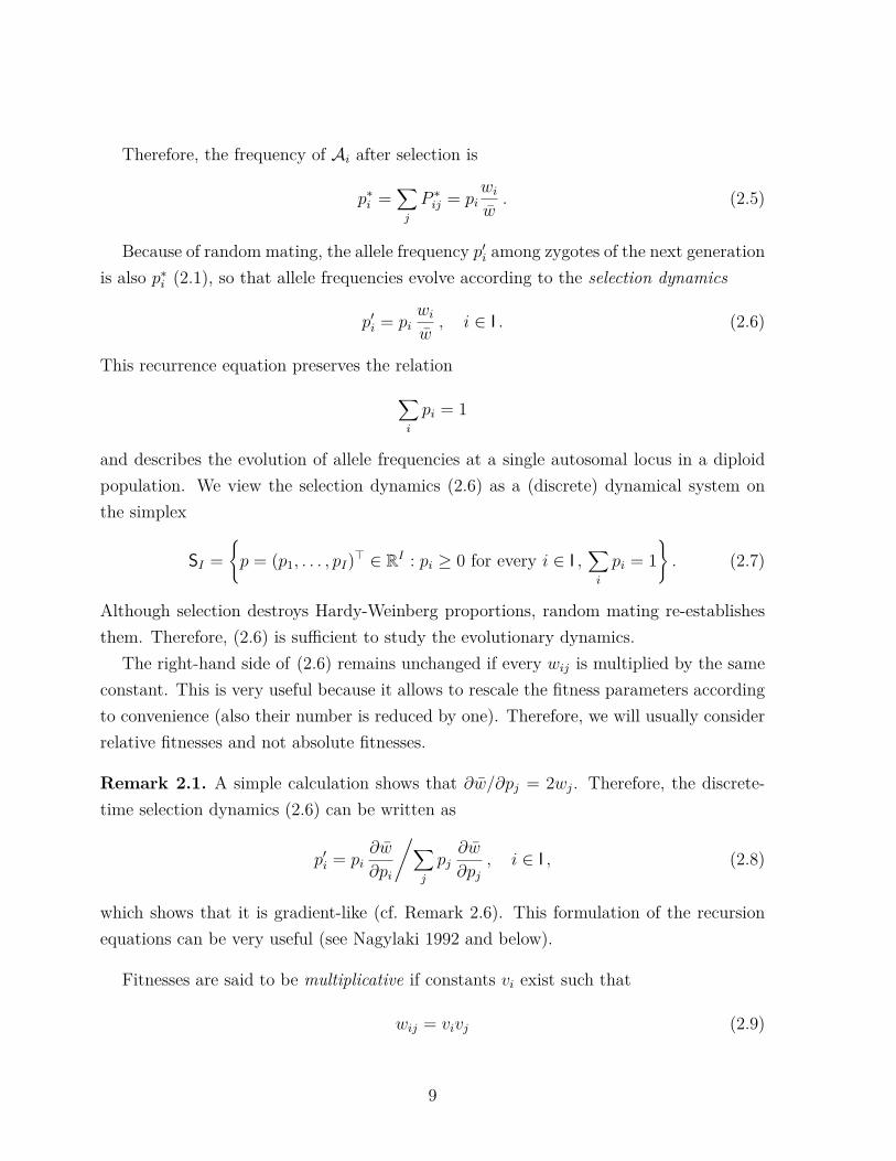
Remark 2.1. A simple calculation shows that ∂w/∂pj = 2wj. Therefore, the discrete-time selection dynamics (2.6) can be written as

p′i = pi∂w

∂pi

/∑j

pj∂w

∂pj, i ∈ I , (2.8)

which shows that it is gradient-like (cf. Remark 2.6). This formulation of the recursionequations can be very useful (see Nagylaki 1992 and below).

Fitnesses are said to be multiplicative if constants vi exist such that

wij = vivj (2.9)

9

for every i, j. Then wi = viv, where v = ∑i vipi, and w = v2. Therefore, (2.6) simplifies

top′i = pi

viv, i ∈ I , (2.10)

which can be solved explicitly because it is equivalent to the linear system x′i = vixi. It iseasy to show that (2.10) also describes the dynamics of a haploid population if the fitnessvi is assigned to allele Ai.

Fitnesses are said to be additive if constants vi exist such that

wij = vi + vj (2.11)

for every i, j. Then wi = vi+ v, where v = ∑i vipi, and w = 2v. Although this assumption

is important (it means absence of dominance; see Sect. 2.3), it does not yield an explicitsolution of the selection dynamics.

Example 2.2. Selection is very efficient. We assume (2.9). Then the solution of (2.10)is

pi(t) = pi(0)vti∑j pj(0)vtj

. (2.12)

Suppose that there are only two alleles, A1 and A2. If A1 is the wild type and A2 is anew beneficial mutant, we may set (without loss of generality!) v1 = 1 and v2 = 1 + s.Then we obtain from (2.12):

p2(t)p1(t) = p2(0)

p1(0)

(v2

v1

)t= p2(0)p1(0)(1 + s)t . (2.13)

Thus, A2 increases exponentially relative to A1.For instance, if s = 0.5, then after 10 generations the frequency of A2 has increased by

a factor of (1 + s)t = 1.510 ≈ 57.7 relative to A1. If s = 0.05 and t = 100, this factor is(1 + s)t = 1.05100 ≈ 131.5. Therefore, slight fitness differences may have a big long-termeffect, in particular, since 100 generations are short on an evolutionary time scale.

Remark 2.3. In haploids, the best allele becomes fixed. To show this, assume that A1

has higher fitness than all other alleles (v1 > vi for every i , 1). Then (vj/v1)t → 0 forj , 1 as t → ∞. Therefore, (2.12) shows that p1(t) → 1 as t → ∞, i.e., in the long runthe best allele becomes fixed. As we shall see below, this is not necessarily so in diploids.

10

Schematic selection dynamics with two alleles

p0 1

10 ,10 ≤≤<< hs

10 ,10 ≤≤<< hs

0 ,10 <<< hs

1 ,10 ><< hs

Figure 2.1: Convergence patterns for selection with two alleles.

2.3 Two alleles and the role of dominance

For the purpose of illustration, we work out the special case of two alleles. We write pand 1− p instead of p1 and p2. Further, we use relative fitnesses and assume

w11 = 1 , w12 = 1− hs , w22 = 1− s , (2.14)

where s is called the selection coefficient and h describes the degree of dominance. Weassume s > 0.

The allele A1 is called dominant if h = 0, partially dominant if 0 < h < 12 , recessive if

h = 1, and partially recessive if 12 < h < 1. No dominance refers to h = 1

2 . Absence ofdominance is equivalent to additive fitnesses (2.11). If h < 0, there is overdominance orheterozygote advantage. If h > 1, there is underdominance or heterozygote inferiority.

From (2.4), the marginal fitnesses of the two alleles are

w1 = 1− hs+ hsp and w2 = 1− s+ s(1− h)p

and, from (2.3), the mean fitness is

w = 1− s+ 2s(1− h)p− s(1− 2h)p2 .

It is easily verified that the allele-frequency change from one generation to the next canbe written as

∆p = p′ − p = p(1− p)sw

[1− h− (1− 2h)p] (2.15a)

= p(1− p)2w

dwdp . (2.15b)

11

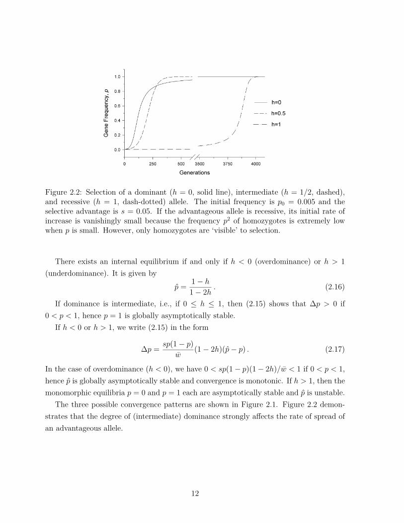
Figure 2.2: Selection of a dominant (h = 0, solid line), intermediate (h = 1/2, dashed),and recessive (h = 1, dash-dotted) allele. The initial frequency is p0 = 0.005 and theselective advantage is s = 0.05. If the advantageous allele is recessive, its initial rate ofincrease is vanishingly small because the frequency p2 of homozygotes is extremely lowwhen p is small. However, only homozygotes are ‘visible’ to selection.

There exists an internal equilibrium if and only if h < 0 (overdominance) or h > 1(underdominance). It is given by

p = 1− h1− 2h . (2.16)

If dominance is intermediate, i.e., if 0 ≤ h ≤ 1, then (2.15) shows that ∆p > 0 if0 < p < 1, hence p = 1 is globally asymptotically stable.

If h < 0 or h > 1, we write (2.15) in the form

∆p = sp(1− p)w

(1− 2h)(p− p) . (2.17)

In the case of overdominance (h < 0), we have 0 < sp(1− p)(1− 2h)/w < 1 if 0 < p < 1,hence p is globally asymptotically stable and convergence is monotonic. If h > 1, then themonomorphic equilibria p = 0 and p = 1 each are asymptotically stable and p is unstable.

The three possible convergence patterns are shown in Figure 2.1. Figure 2.2 demon-strates that the degree of (intermediate) dominance strongly affects the rate of spread ofan advantageous allele.

12

2.4 Summary of results for an arbitrary number of alleles

An important property of (2.6) is that mean fitness is nondecreasing along trajectories(solutions), i.e.,

w′ = w(p′) ≥ w(p) = w , (2.18)

and equality holds if and only if p is an equilibrium.5

A particularly elegant proof of (2.18) was provided by Kingman (1961); see also Nagy-laki (1992, p. 58). The inequality (2.18) shows that w is a Lyapunov function. This hasa number of important consequences. For instance, complex dynamical behavior such aslimit cycles or chaos can be excluded (see below).

The statement (2.18) is closely related to Fisher’s Fundamental Theorem of NaturalSelection, which Fisher (1930) formulated as follows:

“The rate of increase in fitness of any organism at any time is equalto its genetic variance in fitness at that time.”

Here, the additive genetic variance in fitness is defined as the variance of the marginalallelic fitnesses, i.e.,

σ2A = 2

∑i

pi(wi − w)2 . (2.19)

In general, σ2A < σ2

G = ∑i,j pipj(wij − w)2, where σ2

G is the total genetic variance.The classical interpretation of Fisher’s Fundamental Theorem has been that

∆w = σ2A/w , (2.20)

at least approximately. Unless there is no dominance, (2.20) does generally not holdexactly. The following has been proved (Nagylaki 1991):

∆w = σ2A

w(1 + E) , (2.21)

where |E| ≤ 12s and s = maxij wij

minij wij − 1 is the selection intensity. For discussion of this andother interpretations of the FTNS, which may be closer to what Fisher meant, see Burger(2011) and Ewens and Lessard (2015).

From (2.6) it is obvious that the equilibria are precisely the solutions of

pi(wi − w) = 0 for every i ∈ I . (2.22)5p is called an equilibrium, or fixed point, of the recurrence equation p′ = f(p) if f(p) = p. We use

the term equilibrium point to emphasize that we consider an equilibrium that is a single point. The termequilibrium may also refer to a (connected) manifold of equilibrium points.

13

We call an equilibrium internal, or fully polymorphic, if pi > 0 for every i (all alleles arepresent). The I equilibria defined by pi = 1 are called monomorphic because only oneallele is present.

The following result summarizes a number of important properties of the selectiondynamics. Proofs and references to the original literature may be found in Burger (2000,Chap. I.9); see also Lyubich (1992, Chap. 9).

Theorem 2.4. 1. If an isolated internal equilibrium exists, then it is uniquely determined.2. p is an equilibrium if and only if p is a critical point of the restriction of mean

fitness w(p) to the minimal subsimplex of SI that contains the positive components of p.3. If the number of equilibria is finite, then it is bounded above by 2I − 1.4. An internal equilibrium is asymptotically stable if and only if it is an isolated local

maximum of w. Moreover, it is isolated if and only if it is hyperbolic (i.e., the Jacobianhas no eigenvalues of modulus 1).

5. An equilibrium point is stable if and only if it is a local, not necessarily isolated,maximum of w.

6. If an asymptotically stable internal equilibrium exists, then every orbit starting inthe interior of SI converges to that equilibrium.

7. If an internal equilibrium exists, it is stable if and only if, counting multiplicities,the fitness matrix W = (wij) has exactly one positive eigenvalue.

8. If the matrix W has i positive eigenvalues, at least (i− 1) alleles will be absent at astable equilibrium.

9. Every orbit converges to one of the equilibrium points (even if they are not isolated).

2.5 The continuous-time selection model

Most higher animal species have overlapping generations because birth and death occurcontinuously in time. This, however, may lead to substantial complications if one wishesto derive a continuous-time model from biological principles. By contrast, discrete-timemodels can frequently be derived straightforwardly from simple biological assumptions.If evolutionary forces are weak, a continuous-time version can usually be obtained as anapproximation to the discrete-time model.

A rigorous derivation of the differential equations that describe gene-frequency changeunder selection in a diploid population with overlapping generations is a formidable taskand requires a complex model involving age structure (see Nagylaki 1992, Chap. 4.10).

14

Here, we simply state the system of differential equations and justify it in an alternativeway.

In a continuous-time model, the (Malthusian) fitness mij of a genotype AiAj is definedas its birth rate minus its death rate. Then the marginal fitness of allele Ai is

mi =∑j

mijpj ,

the mean fitness of the population is

m =∑i

mipi =∑i,j

mijpipj ,

and the dynamics of allele frequencies becomes

pi = dpidt = pi(mi − m) , i ∈ I .6 (2.23)

This is the analogue of the discrete-time selection dynamics (2.6). Its state space is againthe simplex SI . The equilibria are obtained from the condition pi = 0 for every i. Thedynamics (2.23) remains unchanged if the same constant is added to every mij. We notethat (2.23) is a so-called replicator equation (Hofbauer and Sigmund 1998).

If we setwij = 1 + smij for every i, j ∈ I , (2.24)

where s > 0 is (sufficiently) small, the difference equation (2.6) and the differential equa-tion (2.23) have the same equilibria. This is obvious upon noting that (2.24) implieswi = 1 + smi and w = 1 + sm. Importantly, if the same constant is added to every mij,equation (2.23) remains unchanged. This allows for convenient scaling of the fitnesses.

Following Nagylaki (1992, p. 99), we approximate the discrete model (2.6) by thecontinuous model (2.23) under the assumption of weak selection, i.e., small s in (2.24).We rescale time according to t = bτ/sc, where b c denotes the closest smaller integer.Then s may be interpreted as generation length and, for pi(t) satisfying the differenceequation (2.6), we write πi(τ) = pi(t). Then we obtain formally

dπidτ = lim

s↓0

1s

[πi(τ + s)− πi(τ)] = lims↓0

1s

[pi(t+ 1)− pi(t)] .

From (2.6) and (2.24), we obtain pi(t+ 1)− pi(t) = spi(t)(mi − m)/(1 + sm). Therefore,πi = πi(mi− m) and ∆pi ≈ sπi = spi(mi− m). We note that (2.6) is essentially the Eulerscheme for (2.23).

6Throughout, a dot, ˙ , indicates a derivative with respect to time.

15

The exact continuous-time model reduces to (2.23) only if the mathematically incon-sistent assumption is imposed that Hardy-Weinberg proportions apply for every t whichis generally not true. Under weak selection, however, deviations from Hardy-Weinbergdecay to order O(s) after a short period of time Nagylaki (1992).

Example 2.5. For two alleles, (2.23) simplifies considerably because it is sufficient totrack the allele frequency p = p1.

Scaling the Malthusian parameters in the following way

A1A1 A1A2 A2A20 −hs −s ,

we obtain the simple representation

p = 12sp(1− p)[1− h− (1− 2h)p] , (2.25)

which corresponds to (2.15). This yields the special cases

p = 12sp(1− p) if h = 1

2 (no dominance) (2.26)

andp = sp(1− p)2 if h = 0 (A1 is dominant) . (2.27)

Equation (2.26) is also obtained for a haploid population in which A2 has a selectivedisadvantage of 1

2s relative to A1.

We return to the equation (2.23) for an arbitrary number I of alleles. One of theadvantages of models in continuous time is that they lead to differential equations, andusually these are easier to analyze because the formalism of calculus is available. Anexample for this is that, in continuous time, (2.18) simplifies to

˙m ≥ 0 , (2.28)

which is much easier to prove than (2.18):

˙m = 2∑i,j

mijpj pi = 2∑i

mipi = 2∑i

(m2i − m2)pi = 2

∑i

(mi − m)2pi.

Remark 2.6. We note that the continuous selection dynamics (2.23) is in fact a gener-alized gradient system, whence all trajectories are perpendicular to the level surfaces ofthe associated potential (with respect to an appropriate metric) and converge to a set ofequilibrium points. For this purpose, we define the entries

gij(p) = 12pi(δij − pj) (2.29)

16

of the I × I matrix G(p), where δij is the Kronecker delta. This matrix is symmetric andpositive definite. A simple calculation shows that ∂m

∂pj= 2mj. Therefore, (2.23) can be

written aspi =

I∑j=1

gij∂m

∂pj, i ∈ I , (2.30)

or, in matrix form,p = G(p)∇m , (2.31)

where ∇ denotes the gradient (nabla) operator. Gradient systems on the simplex SI ofthe form (2.31) are often called Svirezhev-Shahshahani gradients after the mathematicianswho introduced them independently (Svireshev 1972, Shahshahani 1989). Using (2.31),we infer immediately that

˙m = (∇m)T p = (∇m)TG(p)∇m ≥ 0 . (2.32)

The corresponding metric assigns to a vector d of gene-frequency changes from p to p+ d

(i.e., ∑i di = 0) the length ||d||p =√dTG(p)−1d =

√∑i d

2i /pi (see Burger 2000, pp.

41–44, and the references there).

3 The general migration-selection model

We assume a population of diploid organisms with discrete, nonoverlapping generations.This population is subdivided into Γ demes (niches). Viability selection acts within eachdeme and is followed by adult migration (dispersal). After migration random matingoccurs within each deme. We assume that the genotype frequencies are the same inboth sexes (e.g., because the population is monoecious). We also assume that, in everydeme, the population is so large that gene and genotype frequencies may be treated asdeterministic, i.e., we ignore random genetic drift.

3.1 Motivation: Geographic structure

Coarse geographic structure means that organisms live in a fragmented, environmentallyheterogeneous habitat and migrate between patches. This leads to population subdivi-sion. If, however, the environment changes smoothly and there are no barriers, geographicstructure changes gradually and migration can be modeled by diffusion (or similar pro-cesses). Populations adapting to spatially heterogeneous environments often experiencegene flow, caused by migration, which may counter adaptation to the local environmentand divergence between subpopulations.

17

subpopulation β

subpopulation α

migration rate: mαβ

cold

hotdiffusion

Figure 3.1: Coarse vs. gradual geographic structure

Population-genetic models for a coarse geographic structure are typically formulatedby difference (or differential) equations and migration is described by a matrix. For agradual geographic structure, partial differential equations, related to reaction-diffusionequations, are the most prominent models. We start with a general approach to modelsin discrete space and postpone the treatment of PDE models to later chapters.

3.2 The recurrence equations

As before, we consider a single locus with I alleles Ai (i ∈ I). Throughout, we use lettersi, j to denote alleles, and greek letters α, β to denote demes. We write G = 1, . . . ,Γ forthe set of all demes. The presentation below is based on Chapter 6.2 of Nagylaki (1992).

We denote the frequency of allele Ai in deme α by pi,α. Therefore, we have∑i

pi,α = 1 (3.1)

for every α ∈ G. Because selection may vary among demes, the fitness (viability) wij,αof an AiAj individual in deme α may depend on α. The marginal fitness of allele Ai indeme α and the mean fitness of the population in deme α are

wi,α =∑j

wij,αpj,α and wα =∑i,j

wij,αpi,αpj,α , (3.2)

respectively.Next, we describe migration. Let mαβ denote the probability that an individual in deme

α migrates to deme β, and let mαβ denote the probability that an (adult) individual in

18

deme α immigrated from deme β. The Γ× Γ matrices

M = (mαβ) and M = (mαβ) (3.3)

are called the forward and backward migration matrices, respectively. Both matrices arestochastic, i.e., they are nonnegative and satisfy

∑β

mαβ = 1 and∑β

mαβ = 1 for every α . (3.4)

Thus, we have assumed that migration probabilities are independent of genotype and noindividuals are lost during migration.

Given the backward migration matrix and the fact that random mating within eachdemes does not change the allele frequencies, the allele frequencies in the next generationare

p′i,α =∑β

mαβp∗i,β , (3.5a)

wherep∗i,α = pi,α

wi,αwα

(3.5b)

describes the change due to selection alone; cf. (2.6). These recurrence equations definea dynamical system on the Γ-fold Cartesian product SΓ

I of the simplex SI .The difference equations (3.5) require that the backward migration rates are known. In

the following, we derive their relation to the forward migration rates and discuss conditionswhen selection or migration do not change the deme proportions.

3.3 The relation between forward and backward migration rates

To derive this relation, we describe the life cycle explicitly. It starts with zygotes onwhich selection acts (possibly including population regulation). After selection adultsmigrate and usually there is population regulation after migration (for instance becausethe number of nesting places is limited). By assumption, population regulation does notchange genotype frequencies. Finally, there is random mating and reproduction, whichneither changes gene frequencies (Section 2.1) nor deme proportions. The respectiveproportions of zygotes, pre-migration adults, post-migration adults, and post-regulationadults in deme α are cα, c∗α, c∗∗α , and c′α:

Zygote - Adult - Adult - Adult - Zygoteselection migration regulation reproduction

cα , pi,α c∗α , p∗i,α c∗∗α , p

′i,α c′α , p

′i,α c′α , p

′i,α

19

Because no individuals are lost during migration, the following must hold:

c∗∗β =∑α

c∗αmαβ , (3.6a)

c∗α =∑β

c∗∗β mβα . (3.6b)

The (joint) probability that an adult is in deme α and migrates to deme β can be expressedin terms of the forward and backward migration rates as follows:

c∗αmαβ = c∗∗β mβα . (3.7)

Inserting (3.6a) into (3.7), we obtain the desired connection between the forward and thebackward migration rates:

mβα = c∗αmαβ∑γ c∗γmγβ

. (3.8)

Therefore, if M is given, an ansatz for the vector c∗ = (c∗1, . . . , c∗Γ)> in terms of c =(c1, . . . , cΓ)> is needed to compute M (as well as a hypothesis for the variation, if any, ofc).

Two frequently used assumptions are the following (Christiansen 1975).1) Soft selection. This assumes that the fraction of adults in every deme is fixed, i.e.,

c∗α = cα for every α ∈ G . (3.9)

This may be a good approximation if the population is regulated within each deme, e.g.,because individuals compete for resources locally (Dempster 1955).

2) Hard selection. Following Dempster (1955), the fraction of adults will be propor-tional to mean fitness in the deme if the total population size is regulated. This has beencalled hard selection and is defined by

c∗α = cαwα/w , (3.10)

wherew =

∑α

cαwα (3.11)

is the mean fitness of the total population.Essentially, these two assumptions are at the extremes of a broad spectrum of possi-

bilities. Soft selection will apply to plants; for animals many schemes are possible.Under soft selection, (3.8) becomes

mβα = cαmαβ∑γ cγmγβ

. (3.12)

20

As a consequence, if c is constant (c′ = c), M is constant if and only if M is constant.If there is no population regulation after migration, then c will generally depend on timebecause (3.6a) yields c′ = c∗∗ = M>c. Therefore, the assumption of constant demeproportions, c′ = c, will usually require that population control occurs after migration.

A migration pattern that does not change deme proportions (c∗∗α = c∗α) is called con-servative. Under this assumption, (3.7) yields

c∗αmαβ = c∗βmβα (3.13)

and, by stochasticity of M and M , we obtain

c∗β =∑α

c∗αmαβ and c∗α =∑β

c∗βmβα . (3.14)

If there is soft selection and the deme sizes are equal (c∗α = cα ≡ constant), then mαβ =mβα.

Remark 3.1. Conservative migration has two interesting special cases.1) Dispersal is called reciprocal if the number of individuals that migrate from deme α

to deme β equals the number that migrate from β to α:

c∗αmαβ = c∗βmβα . (3.15)

If this holds for all pairs of demes, then (3.6a) and (3.4) immediately yield c∗∗β = c∗β.From (3.7), we infer mαβ = mαβ, i.e., the forward and backward migration matrices areidentical.

2) A migration scheme is called doubly stochastic if∑α

mαβ = 1 for every β . (3.16)

If demes are of equal size, then (3.6a) shows that c∗∗α = c∗α. Hence, with equal deme sizesa doubly stochastic migration pattern is conservative. Under soft selection, deme sizesremain constant without further population regulation. Hence, mαβ = mβα and M is alsodoubly stochastic.

Doubly stochastic migration patterns arise naturally if there is a periodicity, e.g., be-cause the demes are arranged in a circular way. If we posit equal deme sizes and homoge-neous migration, i.e., mαβ = mβ−α so that migration rates depend only on distance, thenthe backward migration pattern is also homogeneous because mαβ = mβα = mα−β and,hence, depends only on β−α. If migration is symmetric, mαβ = mβα, and the deme sizesare equal, then dispersion is both reciprocal and doubly stochastic.

21

Juvenile migration is of importance for many marine organisms and plants, where seedsdisperse. It can be treated in a similar way as adult migration. Also models with bothjuvenile and adult migration have been studied. Some authors investigated migrationand selection in dioecious populations, as well as selection on X-linked loci (e.g. Nagylaki1992, pp. 143, 144).

3.4 Migration and selection in continuous time

Following Nagylaki and Lou (2007), we assume that both selection and migration areweak, so that evolution is slow because per-generation changes in allele frequencies aresmall. Then we can approximate the discrete migration-selection dynamics (3.5) by adifferential equation which is easier accessible. Accordingly, let

wij,α = 1 + εrij,α (3.17a)

andmαβ = δαβ + εµαβ , (3.17b)

where rij,α and µαβ are fixed for every i, j ∈ I and every α, β ∈ G, and ε > 0 is sufficientlysmall. From (3.2) we deduce

wi,α = 1 + εri,α and wα = 1 + εrα , (3.18a)

whereri,α =

∑j

rij,αpj,α and rα =∑i,j

rij,αpi,αpj,α . (3.18b)

To approximate the backward migration matrix M , note that (3.10) and (3.18a) implythat, for both soft and hard selection,

c∗α = cα +O(ε) (3.19)

as ε→ 0. Substituting (3.17b) into (3.8) yields

mαα = c∗α(1 + εµαα)c∗α + ε

∑γ c∗γµγα

= 1+εµαα−ε

c∗α

∑γ

c∗γµγα+O(ε2) = 1+ ε

cα(cαµαα−

∑γ

cγµγα)+O(ε2)

because c∗γ/c∗α = cγ/cα +O(ε) by (3.19). Similarly, if α , β, then

mβα = c∗αεµαβc∗β + ε

∑γ c∗γµγβ

= εc∗αc∗βµαβ +O(ε2) = ε

cαcβµαβ +O(ε2) .

22

Defining

µαβ = 1cα

(cβµβα − δαβ

∑γ

cγµγα

), (3.20)

leads tomαβ = δαβ + εµαβ +O(ε2) (3.21)

as ε→ 0.Because M is stochastic, we obtain for every α ∈ Γ,

µαβ ≥ 0 for every β , α and∑β

µαβ = 0 . (3.22)

As a simple consequence of (3.20), µαβ shares the same properties.The final step in our derivation is to rescale time as in Sect. 2.5 by setting t = bτ/εc

and πi,α(τ) = pi,α(t). Inserting all this into the difference equations (3.5) and expandingyields

πi,α(τ + ε) = πi,α 1 + ε[ri,α(π·,α)− rα(π·,α)]+ ε∑β

µαβπi,β +O(ε2) (3.23)

as ε→ 0, where π·,α = (π1,α, . . . , πI,α)> ∈ SI . Rearranging and letting ε→ 0, we arrive at

dπi,αdτ =

∑β

µαβπi,β + πi,α[ri,α(π·,α)− rα(π·,α)] . (3.24)

Absorbing ε into the migration rates and selection coefficients and returning to p(t), weobtain the slow-evolution approximation of (3.5),

pi,α =∑β

µαβpi,β + pi,α[ri,α(p·,α)− rα(p·,α)] . (3.25)

In contrast to the discrete-time dynamics (3.5), here the migration and selection terms aredecoupled. This is a general feature of many other slow-evolution limits (such as mutationand selection, or selection, recombination and migration). Because of the decoupling ofthe selection and migration terms, the analysis of explicit models is often facilitated.

With multiple alleles, there are few general results on the dynamics of (3.25). For twoalleles, we set pα = p1,α and write (3.25) in the form

pα =∑β

µαβpβ + ϕα(pα) . (3.26)

Since µαβ ≥ 0 whenever α , β, the system (3.26) is quasimonotone or cooperative, i.e.,∂pα/∂pβ ≥ 0 if α , β. As a consequence, (3.26) cannot have an exponentially stable limit

23

cycle. However, Akin (personal communication) has proved for three diallelic demes thata Hopf bifurcation can produce unstable limit cycles. This precludes global convergence,though not generic convergence. If Γ = 2, then every trajectory converges (Hirsch 1982;Hadeler and Glas 1983; see also Hofbauer and Sigmund 1998, p. 28).

3.5 Important special migration patterns

We shall introduce several migration patterns that play an important role in the pop-ulation genetics and ecological literature. We start with the arguably simplest model,introduced by Haldane (1930) who studied various aspects of it; see also Wright (1931).

3.5.1 The continent-island model

We consider a population living on an island. Each generation, a proportion a of adultsis removed by mortality or emigration and a fraction b of migrants with constant allelicfrequencies qi is added. A simple interpretation is that of unidirectional migration from acontinent to an island. The continental population is assumed to be in equilibrium withallele frequencies qi > 0. If there is backmigration to the continent and the populationsize on the continent exceeds that on the island sufficiently, then changes in qi due tobackmigration can be ignored. Sometimes, qi is interpreted as the average frequency over(infinitely) many islands and the model is simply called the island model.

We denote the fraction of zygotes on the island with immigrant parents by m =b/(1−a+b). This corresponds to the backward migration rate. Interpreting the continentas deme 2 and the island as deme 1, we obtain the dynamics of allele frequencies pi onthe island from (3.5):

p′i = (1−m)piwiw

+mqi . (3.27)

Here, wi is the marginal fitness of allele Ai on the island, w the mean fitness of theisland population, and subscripts indicating the deme have been dropped. Throughoutwe assume 0 < m < 1.

Remark 3.2. If we define uij = mqj and consider uij as the mutation rate from Ai toAj, a special case of the (multiallelic) mutation-selection model is obtained (the so-calledhouse-of-cards model). Therefore (Burger 2000, pp. 102-103), (3.27) has the Lyapunovfunction

V (p) = w(p)1−m∏i

p2mqii , (3.28)

24

Table 3.1: Water snakes (Nerodia sipedon) in Lake Erie come in two forms: the bandedmainland morph (left) and the gray island morph (right). The mainland morph migratesto the islands in the lake, but the island morph has never been observed on the mainland(King and Lawson 1995).

a fact that is straightforward to check. It follows that all trajectories are attracted by theset of equilibria.

Clearly, no allele carried to the island recurrently by immigrants can be lost. Therefore,we focus our attention on the diallelic case, in which one allele is carried to the island andon the island a new, mutant type has occurred that has a selective advantage over theimmigrant, i.e., it improves local adaptation of its carriers. We determine the conditionsunder which this ‘island allele’ persists in the population despite immigration of thedeleterious alleles from the continent. This model is very useful to study the conditionsunder which local adaptation in peripheral populations, e.g., on an island, in a cave or adesert, can occur. Such continent-island scenarios do indeed occur in nature. A prominentand well studied example are water snakes inhabiting the shores of Lake Erie, wherethe mainland population corresponds to the continental population and the populationliving on the lake’s islands to that on the island (see Figure 3.5.1). Based on empiricalestimates of gene flow, population size, and selection, King and Lawson (1995) concludethat based on initial population subdivision (after the glaciers receded), natural selectionhas subsequently carried island populations toward a new adaptive peak.

To study the diallelic case, we consider alleles A1 and A2 with frequencies p and 1− pon the island, and q2 = 1 on the continent. Thus, all immigrants are A2A2. Therefore,A1 evolves according to

p′ = (1−m)pw1

w. (3.29)

25

IslandGenotypes Fitnesses

Con

tinen

tA2

A1A1 sm

A1 is a beneficial mutant(s>0)

A1A2 hsA2A2 -s

is fixed for

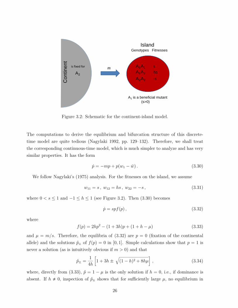
Figure 3.2: Schematic for the continent-island model.

The computations to derive the equilibrium and bifurcation structure of this discrete-time model are quite tedious (Nagylaki 1992, pp. 129–132). Therefore, we shall treatthe corresponding continuous-time model, which is much simpler to analyze and has verysimilar properties. It has the form

p = −mp+ p(w1 − w) . (3.30)

We follow Nagylaki’s (1975) analysis. For the fitnesses on the island, we assume

w11 = s , w12 = hs , w22 = −s , (3.31)

where 0 < s ≤ 1 and −1 ≤ h ≤ 1 (see Figure 3.2). Then (3.30) becomes

p = spf(p) , (3.32)

wheref(p) = 2hp2 − (1 + 3h)p+ (1 + h− µ) (3.33)

and µ = m/s. Therefore, the equilibria of (3.32) are p = 0 (fixation of the continentalallele) and the solutions p± of f(p) = 0 in [0, 1]. Simple calculations show that p = 1 isnever a solution (as is intuitively obvious if m > 0) and that

p± = 14h

[1 + 3h±

√(1− h)2 + 8hµ

], (3.34)

where, directly from (3.33), p = 1 − µ is the only solution if h = 0, i.e., if dominance isabsent. If h , 0, inspection of p± shows that for sufficiently large µ, no equilibrium in

26

a)

Scaled migration rate, m/s

Alle

le fr

eque

ncy,

p

100

1

100

1

b)

Scaled migration rate, m/s

Alle

le fr

eque

ncy,

p

2

Figure 3.3: Bifurcation structure of the continent-island model. Bold lines representasymptotically stable equlibria, dashed lines represent unstable equilibria. a) −1

3 ≤ h ≤ 1;b) −1 ≤ h < −1

3 (A1 nearly or completely recessive).

[0, 1] exists, thus polymorphism cannot be maintained at all. The stability properties ofthe equilibria are determined by the sign of f(p).

Simple analysis of p± and f(p) shows that there are two qualitatively different cases.(i) If h ≥ −1

3 , the nontrivial equilibrium p− is unique and stable when it exists, which isthe case if 0 < µ < µ1 = 1 + h. If µ ↑ µ1, then p− ↓ 0, i.e., the conditions become veryunfavorable for a polymorphism. (ii) If −1 < h < −1

3 , there are two nontrivial equilibriaif µ1 < µ < µ2 = −(1− h)2/(8h), of which only the larger one is stable; if h = −1 (A1 isrecessive), both equilibria exist if µ < 1

2 . These two cases are illustrated in Figure 3.3.There are three main conclusions arising from this analysis. First, if migration is suffi-

ciently strong relative to selection (as determined by s and h), then no polymorphism onthe island can be maintained; the island is swamped by the continental type. Second, ifmigration is sufficiently weak, µ < µ1, then there is a globally stable polymorphic equilib-rium and differentiation between the continent and the island population is established.This differentiation increases with decreasing µ. Third, if the locally advantageous islandallele A1 is nearly or completely recessive and migration is intermediate (µ1 < µ < µ2),then establishment of a polymorphism is only possible if the initially A1 is sufficientlyfrequent.

3.5.2 Two diallelic demes without dominance in continuous time

We consider a diallelic locus and bi-directional migration between two demes. In addition,we assume continuous time, i.e., (3.25), and absence of dominance. A global analysis ofthis model was provided by Eyland (1971), whom we folllow. We assume that the fitnesses

27

(rij,α) of A1A1, A1A2, and A2A2 in deme α are sα, 0, and −sα, respectively, where sα , 0(α = 1, 2). Moreover, we set µ1 = µ12 > 0, µ2 = µ21 > 0, and write pα for the frequencyof A1 in deme α. Then (3.25) becomes

p1 = µ1(p2 − p1) + s1p1(1− p1) , (3.35a)

p2 = µ2(p1 − p2) + s2p2(1− p2) . (3.35b)

The equilibria can be calculated explicitly. At equilibrium, p1 = 0 if and only if p2 = 0(global loss of A1), and p1 = 1 if and only if p2 = 1 (global fixation of A1). In addition,there may be an internal equilibrium point. We set

σα = µαsα

, κ = σ1 + σ2 , (3.36)

andB =

√1− 4σ1σ2 . (3.37)

Then it is straightforward to show that the internal equilibrium exists if and only ifs1s2 < 0 and |κ| < 1. If s2 < 0 < s1, it is given by

p1 = 12(1 +B)− σ1 and p2 = 1

2(1−B)− σ2 . (3.38)

Therefore, diversifying or divergent selection in the demes is necessary to maintain poly-morphism.

It is straightforward to determine the local stability properties of the three possibleequilibria. For instance, at the equilibrium (0, 0) the trace and determinant of the Jacobianare given by s1 +s2−µ1−µ2 and s1s2(1−κ), respectively. It follows that (0, 0) is linearlystable if either s1 < 0 and s2 < 0 or if s1s2 < 0, s1 + s2 < µ1 + µ2, and κ > 1,where s1 + s2 ≤ 0 < µ1 + µ2 is automatically fulfilled if s1s2 < 0 and κ > 1, hold.The polymorphic equilibrium (3.38) is linearly stable when it exists. In this case, thedeterminant is −s1s2

(1− 4σ1σ2 + (σ1 − σ2)

√1− 4σ1σ2

), which is positive if σ1 > 0,

σ2 < 0, and |κ| < 1. The trace is µ1 + µ2 + (s2 − s1)√

1− 4σ1σ2, which is negative.Gobal asymptotic stability follows from the results cited above about quasimonotone

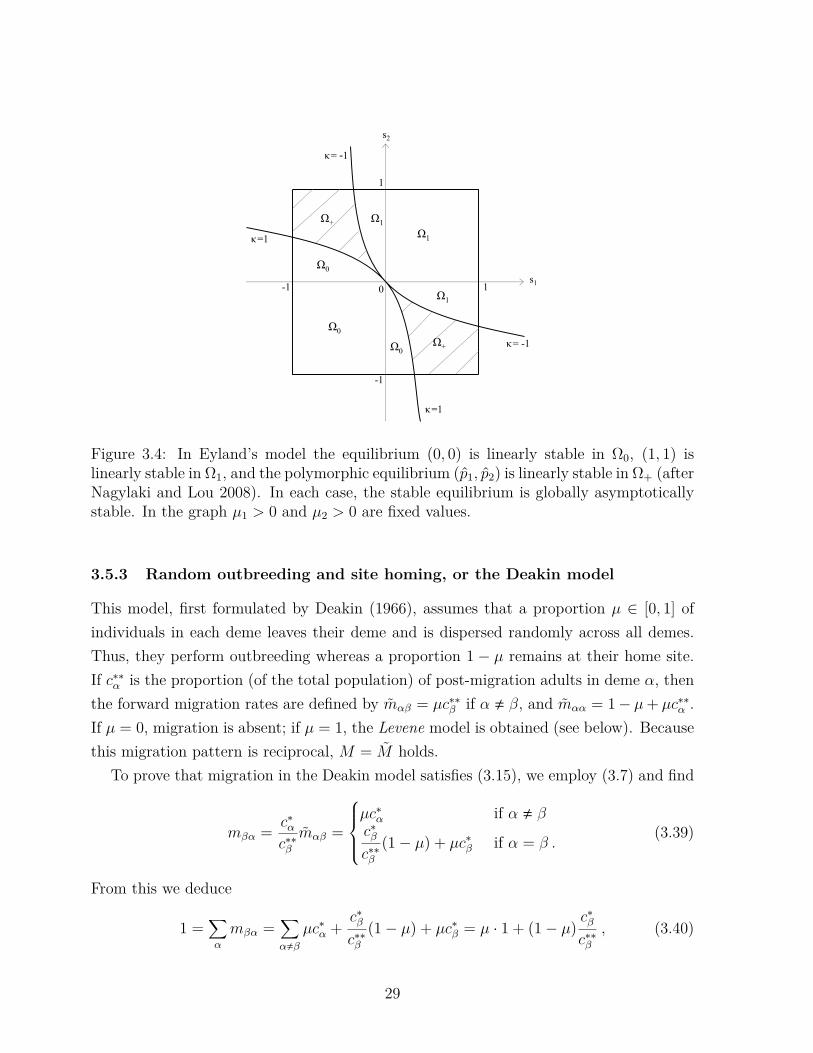
systems. Let p = (p1, p2)>. Then allele A1 is eliminated in the region Ω0 in Figure 3.4,i.e., p(t)→ (0, 0) as t→∞, whereas A1 is ultimately fixed in the region Ω1. In Ω+, p(t)converges globally to the internal equilibrium point p given by (3.38). For the discrete-time model, such a complete analysis is not available. We will treat some aspects of themuch more complex model with dominance in a subsequent section.

Finally, we briefly introduce three types of models to which we shall return in subse-quent sections.

28

s2

0

1

1

=1m2

m1 s1

Fig. 1

s2

0

1

1s1

-1

-1

+

+

1

1

1

0

0

0

=1

=1

= -1

= -1

Fig. 2Figure 3.4: In Eyland’s model the equilibrium (0, 0) is linearly stable in Ω0, (1, 1) islinearly stable in Ω1, and the polymorphic equilibrium (p1, p2) is linearly stable in Ω+ (afterNagylaki and Lou 2008). In each case, the stable equilibrium is globally asymptoticallystable. In the graph µ1 > 0 and µ2 > 0 are fixed values.

3.5.3 Random outbreeding and site homing, or the Deakin model

This model, first formulated by Deakin (1966), assumes that a proportion µ ∈ [0, 1] ofindividuals in each deme leaves their deme and is dispersed randomly across all demes.Thus, they perform outbreeding whereas a proportion 1 − µ remains at their home site.If c∗∗α is the proportion (of the total population) of post-migration adults in deme α, thenthe forward migration rates are defined by mαβ = µc∗∗β if α , β, and mαα = 1− µ+ µc∗∗α .If µ = 0, migration is absent; if µ = 1, the Levene model is obtained (see below). Becausethis migration pattern is reciprocal, M = M holds.

To prove that migration in the Deakin model satisfies (3.15), we employ (3.7) and find

mβα = c∗αc∗∗βmαβ =

µc∗α if α , βc∗βc∗∗β

(1− µ) + µc∗β if α = β .(3.39)

From this we deduce

1 =∑α

mβα =∑α,β

µc∗α +c∗βc∗∗β

(1− µ) + µc∗β = µ · 1 + (1− µ)c∗βc∗∗β

, (3.40)

29

which immediately yields c∗∗β = c∗β for every β provided µ < 1. Therefore, we obtainmβα = µc∗α if α , β and c∗βmβα = c∗βµc

∗α = c∗αmαβ, i.e., reciprocity.

We will always assume soft selection in the Deakin model, i.e., c∗α = cα. Thus, for agiven (probability) vector c = (c1, . . . , cΓ)>, the single parameter µ is sufficient to describethe migration pattern:

mβα = mβα =

µcα if α , β1− µ+ µcβ if α = β .

(3.41)

If all demes have the same size, the so-called island model is obtained. Then migration isusually scaled such that individuals stay in their home deme with probability 1−m andmigrate to each of the other demes with probability m/(Γ− 1).

3.5.4 The Levene model

The Levene model (Levene 1953) assumes soft selection and

mαβ = cβ . (3.42)

Thus, dispersing individuals are distributed randomly across all demes in proportion tothe deme sizes. In particular, migration is independent of the deme of origin and M = M .

Alternatively, the Levene model could be defined by mαβ = µβ, where µβ > 0 areconstants satisfying ∑β µβ = 1. Then (3.8) yields mαβ = c∗β for every α, β ∈ G. Withsoft selection, we get mαβ = cβ. This is all we need if demes are regulated to constantproportions. But the proportions remain constant even without regulation, for (3.6a)gives c′α = c∗∗α = µα. This yields the usual interpretation µα = cα (Nagylaki 1992, Sect.6.3).

An equivalent interpretation is that the adults form a common mating pool. Effectively,this models a population occupying a spatially heterogeneous environment, but withoutevolving population structure because of global panmixis.

3.5.5 Stepping-stone model

In the linear stepping-stone model the demes are arranged in a linear order and individualscan reach only one of the neighboring demes. It is an extreme case among migrationpatterns exhibiting isolation by distance, i.e., patterns in which migration diminishes withthe distance from the parental deme. In the classical homogeneous version, the forward

30

migration matrix is

M =

1−m m 0 . . . 0m 1− 2m m 0...

. . ....

0 m 1− 2m m0 . . . 0 m 1−m

. (3.43)

We leave it to the reader to derive the backward migration matrix using (3.8). It is aspecial case of the following general tridiagonal form:

M =

n1 r1 0 . . . 0q2 n2 r2 0...

. . ....

0 qΓ−1 nΓ−1 rΓ−10 . . . 0 qΓ nΓ

, (3.44)

where nα ≥ 0 and qα+nα+rα = 1 for every α, qα > 0 for α ≥ 2, rα > 0 for α ≤ Γ−1, andq1 = rΓ = 0. This matrix admits variable migration rates between neighboring demes.

If all deme sizes are equal, the homogeneous matrix (3.43) satisfies M = M , and eachdeme exchanges a fraction m of the population with each of its neighboring demes. Thestepping-stone model has been used as a starting point to derive the partial differentialequations for selection and dispersal in continuous space (Nagylaki 1989). Also circularand infinite variants have been investigated.

Unless stated otherwise, we assume that the backward migration matrix M is constant,as is the case for soft selection if deme proportions and the forward migration matrix areconstant. Then the recurrence equations (3.5) provide a self-contained description ofthe migration-selection dynamics. Hence, they are sufficient to study evolution for anarbitrary number of generations.

4 Two alleles and finitely many demes

Of central interest is the identification of conditions that guarantee the maintenance ofgenetic diversity. Often it is impossible to determine the equilibrium structure in detailbecause establishing existence and, even more so, stability or location of polymorphicequilibria is unfeasible. Below we introduce an important concept that is particularlyuseful to establish maintenance of genetic variation at diallelic loci. Throughout thissection we consider a single locus with two alleles. The number of demes, Γ, can bearbitrary.

31

4.1 Protected polymorphism

There is a protected polymorphism (Prout 1968) if, independently of the initial condi-tions, a polymorphic population cannot become monomorphic. Essentially, this requiresthat if an allele becomes very rare, its frequency must increase. In general, a protectedpolymorphism is neither necessary nor sufficient for the existence of a stable polymorphicequilibrium. For instance, on the one hand, if there is an internal limit cycle that attractsall solutions, then there is a protected polymorphism. On the other hand, if there aretwo internal equilibria, one asymptotically stable, the other unstable, then selection mayremove one of the alleles if sufficiently rare. A generalization of this concept to multiplealleles would correspond to the concept of permanence often used in ecological models(e.g., Hofbauer and Sigmund 1998).

Because we consider only two alleles, we can simplify the notation. We write pα = p1,α

for the frequency of allele A1 in deme α (and 1 − pα for that of A2 in deme α). Letp = (p1, . . . , pΓ)> denote the vector of allele frequencies. Instead of using the fitnessassignments w11,α, w12,α, and w22,α, it will be convenient to scale the fitness of the threegenotypes in deme α as follows

A1A1 A1A2 A2A2xα 1 yα

(4.1)

(xα, yα ≥ 0). This can be achieved by setting xα = w11,α/w12,α and yα = w22,α/w12,α,provided w12,α > 0.

With these fitness assignments, one obtains

w1,α = 1− pα + xαpα and wα = xαp2α + 2pα(1− pα) + yα(1− pα)2 , (4.2)

and the migration-selection dynamics (3.5) becomes

p∗α = pαw1,α/wα (4.3a)

p′α =∑β

mαβp∗β . (4.3b)

We consider this as a (discrete) dynamical system on [0, 1]Γ.We call allele A1 protected if it cannot be lost. Thus, it has to increase in frequency if

rare. In mathematical terms this means that the monomorphic equilibrium p = 0 mustbe unstable. To derive a sufficient condition for instability of p = 0, we linearize (4.3)at p = 0. If yα > 0 for every α (which means that A2A2 is nowhere lethal), a simple

32

calculation shows that the Jacobian of (4.3a),

D =(∂p∗α∂pβ

) ∣∣∣∣∣∣p=0

, (4.4)

is a diagonal matrix with (nonzero) entries dαα = y−1α . Because (4.3b) is linear, the

linearization of (4.3) isp′ = Qp , where Q = MD , (4.5)

i.e., qαβ = mαβ/yβ.To obtain a simple criterion for protection, we assume that the descendants of indi-

viduals in every deme be able eventually to reach every other deme. Mathematically, theappropriate assumption is that M is irreducible. Then Q is also irreducible and it is non-negative. Therefore, the Theorem of Perron and Frobenius (see Appendix A; a proof maybe found in Seneta 1981) implies the existence of a uniquely determined eigenvalue λ0 > 0of Q such that |λ| ≤ λ0 holds for all eigenvalues of Q. In addition, there exists a strictlypositive eigenvector pertaining to λ0 which, up to multiplicity, is uniquely determined.As a consequence,

A1 is protected if λ0 > 1 and A1 is not protected if λ0 < 1 (4.6)

(if λ0 = 1, then stability cannot be decided upon linearization). As is easy to show, thismaximal eigenvalue satisfies

minα

∑β

qαβ ≤ λ0 ≤ maxα

∑β

qαβ , (4.7)

with equality if and only if all the row sums are the same.

Example 4.1. Suppose that A2A2 is at least as fit as A1A2 in every deme and more fit inat least one deme, i.e., yα ≥ 1 for every α and yβ > 1 for some β. Then qαβ = mαβ/yβ ≤mαβ for every β. Because M is irreducible, there is no β such that mαβ = 0 for every α.Therefore, the row sums ∑β qαβ = ∑

βmαβ/yβ in (4.7) are not all equal to one, and weobtain

λ0 < maxα

∑β

qαβ ≤ maxα

∑β

mαβ = 1 . (4.8)

Thus, A1 is not protected, and this holds independently of the choice of the xα, or w11,α.It can be shown similarly that A1 is protected if A1A2 is favored over A2A2 in at least

one deme and is nowhere less fit than A2A2.

33

One obtains the condition for protection of A2 if, in (4.6), A1 is replaced by A2 and λ0

is the maximal eigenvalue of the matrix with entries mαβ/xβ. Clearly, there is a protectedpolymorphism if both alleles are protected.

In the case of complete dominance the eigenvalue condition (4.6) cannot be satisfied.Consider, for instance, protection of A1 if A2 is dominant, i.e., yα = 1 for every α. Thenqαβ = mαβ, ∑β qαβ = ∑

βmαβ = 1, and λ0 = 1. This case is treated in Section 6.2 of(Nagylaki 1992).

4.2 Two demes

It will be convenient to set

xα = 1− rα and yα = 1− sα , (4.9)

where we assume rα < 1 and sα < 1 for every α ∈ 1, 2. We write the backwardmigration matrix as

M =(

1−m1 m1m2 1−m2

), (4.10)

where 0 < mα < 1 for every α ∈ 1, 2.Now we derive the condition for protection of A1. The characteristic polynomial of Q

is proportional to

ϕ(x) = (1−s1)(1−s2)x2− (2−m1−m2−s1−s2 +s1m2 +s2m1)x+1−m1−m2 . (4.11)

It is convex and satisfies

ϕ(1) = s1s2(1− κ1) , (4.12a)

ϕ′(1) = (1− s1)(m2 − s2) + (1− s2)(m1 − s1) , (4.12b)

whereκ1 = m1

s1+ m2

s2. (4.13)

By Example 4.1, A1 is not protected if A1A2 is less fit than A2A2 in both demes (moregenerally, if s1 ≤ 0, s2 ≤ 0, and s1 + s2 < 0). Of course, A1 will be protected if A1A2 isfitter than A2A2 in both demes (more generally, if s1 ≥ 0, s2 ≥ 0, and s1 + s2 > 0).

Hence, we restrict attention to the most interesting case when A1A2 is fitter thanA2A2 in one deme and less fit in the other, i.e., s1s2 < 0. The Perron-Frobenius Theoreminforms us that ϕ(x) has two real roots. We have to determine when the larger (λ0)

34

s2

0

1

1

=1m2

m1 s1

Fig. 1

s2

0

1

1s1

-1

-1

+

+

1

1

1

0

0

0

=1

=1

= -1

= -1

Fig. 2

Figure 4.1: The region of protection of A1 (hatched) (from Nagylaki and Lou 2008).

satisfies λ0 > 1. Because ϕ′′(x) > 0, this is the case if and only if (i) ϕ(1) < 0 or (ii)ϕ(1) ≥ 0 and ϕ′(1) < 0. By noting that m1 ≥ s1 if κ1 ≥ 1 and s2 < 0, it is straightforwardto show that ϕ(1) ≥ 0 and ϕ′(1) < 0 is never satisfied if s1 > 0 and s2 < 0. By symmetry,this argument also applies to s1 < 0 and s2 > 0, and we can conclude that allele A1 isprotected if ϕ(1) < 0, i.e., if

κ1 < 1 ; (4.14)

cf. (Bulmer 1972). It is not protected if κ1 > 1. Figure 4.1 displays the region of protectionof A1 for given m1 and m2.

An analogous treatment applies to A2. In particular, if r1r2 < 0, then A2 is protectedif

κ2 < 1 , (4.15)

and not protected if κ2 > 1.If there is no dominance (rα = −sα and 0 < |sα| < 1 for α = 1, 2), then further

simplification can be achieved because κ2 = −κ1. From the preceding paragraphs theresults depicted in Figure 3.4 are obtained. Setting κ = κ1, the region of a protectedpolymorphism is

Ω+ = (s1, s2) : s1s2 < 0 and |κ| < 1 . (4.16)

In a panmictic population, a stable polymorphism can not occur in the absence of

35

overdominance. Protection of both alleles in a subdivided population requires that selec-tion in the two demes is in opposite direction and sufficiently strong relative to migration.Therefore, the study of the maintenance of polymorphism is of most interest if selectionacts in opposite direction and dominance is intermediate, i.e.,

rαsα < 0 for α = 1, 2 and s1s2 < 0. (4.17)

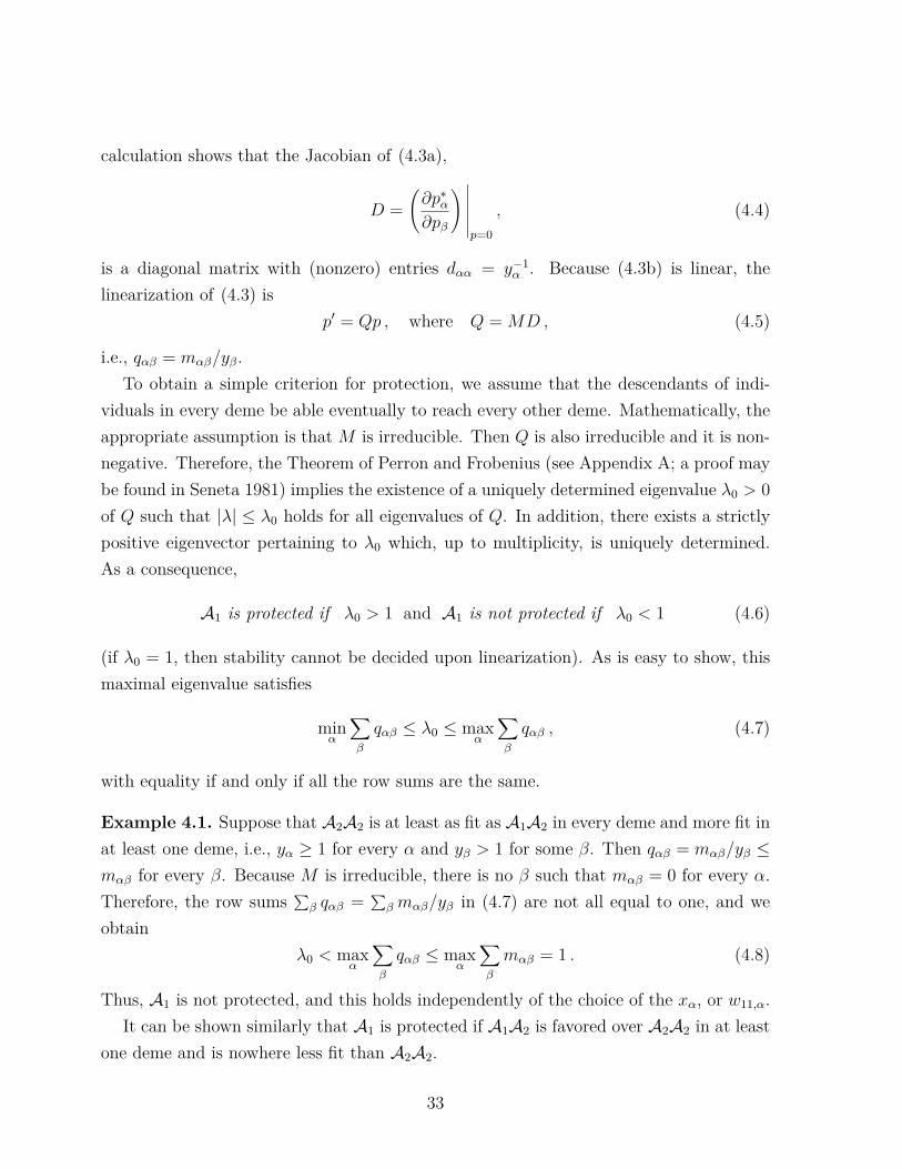
Example 4.2. It is illuminating to study how the parameter region in which a protectedpolymorphism exists depends on the degree of dominance in the two demes. Figures4.2 and 4.3 display the regions of protected polymorphism for two qualitatively differentscenarios of dominance. In the first, the fitnesses are given by

A1A1 A1A2 A2A21 + s 1 + hs 1− s1− as 1− has 1 + as ,

(4.18)

thus, there is deme independent degree of dominance (Nagylaki 2009a). In the secondscenario, the fitnesses are given by

A1A1 A1A2 A2A21 + s 1 + hs 1− s1− as 1 + has 1 + as .

(4.19)

Here, allele Ai is (partially) dominant in deme i (thus, there is dominance-environmentinteraction). In both cases, we assume 0 < s < 1, 0 < a < 1 (a is a measure of theselection intensity in deme 2 relative to deme 1), −1 ≤ h ≤ 1 (intermediate dominance),and m1 = m2 = m. We will show that in these two cases, h has opposite effects on themaintenance of a protected polymorphism.

If, in (4.18), selection is sufficiently symmetric, i.e., a > 1/(1 + 2s), there exists aprotected polymorphism for every h ≤ 1 and every m ≤ 1. Otherwise, for given a, thecritical migration rate m admitting a protected polymorphism decreases with increasing hbecause this increases the average (invasion) fitness of A1. This can be shown analyticallyby studying the principal eigenvalue.

For (4.19), increasing h greatly facilitates a protected polymorphism because it leads toan increase of the average fitness of heterozygotes relative to the homozygotes. The preciseargument is as follows. If we rescale fitnesses in (4.19) according to (4.1), the matrix Q in(4.5) has the entries qα1 = mα1(1+hs)/(1−s) and qα2 = mα2(1+has)/(1−as), which areincreasing in h. Therefore, the principal eigenvalue λ0 of Q increases in h (e.g. Bermanand Plemmons 1994, Chapter 1.3), and (4.6) implies that protection of A1 is facilitatedby increasing h. Because an analogous reasoning applies to A2, the result is proved.

36

0.0 0.2 0.4 0.6 0.8 1.0a

0.1

0.2

0.3

0.4

0.5m

Figure 4.2: Influence of the degree of dominance on the region of protected polymorphism(shaded). The fitness scheme is (4.18) with s = 0.1, and migration is symmetric, i.e.,m1 = m2 = m. The values of h are -0.95, -0.5, 0, 0.5, 0.95 and correspond to thecurves from left to right (light shading to dark shading as h increases). A protectedpolymorphism is maintained in the shaded area to the right of the respective curve. Tothe right of the white vertical line, a protected polymorphism exists for every m.

0.0 0.2 0.4 0.6 0.8 1.0a

0.1

0.2

0.3

0.4

0.5m

Figure 4.3: Influence of the degree of dominance on the region of protected polymorphism(shaded). The fitness scheme is (4.19) with s = 0.1, and migration is symmetric, i.e.,m1 = m2 = m. The values of h are -0.75, -0.25, 0, 0.25, 0.75 and correspond to the curvesfrom right to left (dark shading to light as h increases!). A protected polymorphism ismaintained in the shaded area to the right of the respective curve.

37

Indeed, the above finding on the role of dominance for the fitness scheme (4.19) isa special case of the following result of Nagylaki (personal communication). Assumefitnesses of A1A1, A1A2, and A2A2 in deme α are 1 + sα, 1 + hαsα, and 1, respectively,where sα > −1 and 0 ≤ hα ≤ 1. If the homozygote fitnesses are fixed, increasing theheterozygote fitness in each deme aids the existence of a protected polymorphism. Theproof follows by essentially the same argument as above.

Example 4.3. In the Deakin model, the condition (4.14) for protection of allele A1

becomesκ1 = µ

(c2

s1+ c1

s2

)< 1, (4.20)

where s1s2 < 0. Therefore, for given s1, s2, and c1, there is a critical value µ0 such thatallele A1 is protected if and only if µ < µ0. This implies that for two diallelic demes aprotected polymorphism is favored by a smaller migration rate.

Example 4.4. In the Levene model, the condition for a protected polymorphism is

c2

s1+ c1

s2< 1 and c2

r1+ c1

r2< 1 . (4.21)

We close this subsection with an example showing that already with two alleles andtwo demes the equilibrium structure can be quite complicated.

Example 4.5. In the absence of migration, the recurrence equations for the allele fre-quencies p1, p2 in the two demes are two decoupled one-locus selection dynamics of theform (2.15). Therefore, if there is underdominance in each deme, the top convergencepattern in Figure 2.1 applies to each deme. As a consequence, in the absence of migra-tion, the complete two-deme system has nine equilibria, four of which are asymptoticallystable and the others are unstable. Under sufficiently weak migration all nine equilibriaare admissible and the four stable ones remain stable, whereas the other five are unstable.Two of the stable equilibria are internal. For increasing migration rate, several of theseequilibria are extinguished in a sequence of bifurcations (Karlin and McGregor 1972a).

4.3 Arbitrary number of demes

The following result is a useful tool to study protection of an allele. Let I(n) and Q(n)

respectively designate the n× n unit matrix and the square matrix formed from the firstn rows and columns of Q.

38

Theorem 4.6 (Christiansen 1974). If there exists a permutation of demes such that

det(I(n) −Q(n)) < 0 (4.22)

for some n, where 1 ≤ n ≤ Γ, then A1 is protected.

This theorem is sharp in the sense that if the inequality in (4.22) is reversed for everyn ≤ Γ, then A1 is not protected.

The simplest condition for protection is obtained from Theorem 4.6 by setting n = 1.Hence, A1 is protected if an α exists such that (Deakin 1972)

mαα/yα > 1 . (4.23)

This condition ensures that, when rare, the allele A1 increases in frequency in deme αeven if this subpopulation is the only one containing the allele. The general conditionin the above theorem ensures that A1 increases in the n subpopulations if they are theonly ones that contain it. Therefore, we get the following simple sufficient condition fora protected polymorphism:

There exist α and β such that mαα/yα > 1 and mββ/xβ > 1. (4.24)

If we apply these results to the Deakin model with an arbitrary number of demes,condition (4.24) becomes

There exist α and β such that 1− µ(1− cα)yα

> 1 and 1− µ(1− cβ)xβ

> 1. (4.25)

A more elaborate and less stringent condition follows from Theorem 4.6 by nice matrixalgebra:

Corollary 4.7 (Christiansen 1974). For the Deakin model with Γ ≥ 2 demes, the followingis a sufficient condition for protection of A1. There exists a deme α such that

1− yα ≥ µ (4.26)

or, if (4.26) is violated in every deme α, then

µ∑α

cαµ+ yα − 1 > 1 . (4.27)

If (4.26) is violated for every α and the inequality in (4.27) is reversed, then A1 is notprotected.

39

Corollary 4.7 can be extended to the generalized, or inhomogeneous, Deakin model,which allows for different homing rates (Christiansen 1974; Karlin 1982, pp. 85, 127).Using Corollary 4.7, we can generalize the finding from two diallelic demes that lessoutbreeding is favorable for protection of one or both alleles. More precisely, we show:

Corollary 4.8. If 0 < µ1 < µ2 ≤ 1, then allele A1 is protected for µ1 if µ2 satisfies theconditions in Corollary 4.7.

Proof. If condition (4.26) holds for µ2, it clearly holds for µ1. Now suppose that 1−yα < µ1

for every α (hence 1− yα < µ2) and that µ2 satisfies (4.27). Because

µ∑α

cαµ+ yα − 1 =

∑α

cα(µ+ yα − 1)µ+ yα − 1 −

∑α

cα(yα − 1)µ+ yα − 1 = 1 +

∑α

cα(1− yα)µ+ yα − 1 ,

µ2 satisfies condition (4.27) if and only if∑α

cα(1− yα)µ1 + yα − 1

µ1 + yα − 1µ2 + yα − 1 =

∑α

cα(1− yα)µ2 + yα − 1 > 0 . (4.28)

Because µ1/µ2 ≥ (µ1 + yα − 1)/(µ2 + yα − 1) if and only if yα ≤ 1, we obtain (whether1− µ2 < yα < 1 or yα ≥ 1, where the latter is not possible for every α by Example 4.1)

µ1∑α

cα(1− yα)µ1 + yα − 1 = µ2

∑α

cα(1− yα)µ2 + yα − 1

µ2 + yα − 1µ1 + yα − 1

µ1

µ2≥ µ2

∑α

cα(1− yα)µ2 + yα − 1 > 0 , (4.29)

which proves our assertion.

Karlin (1982, p. 128) extended this result to migration matrices of the form

M (µ) = (1− µ)I + µM , (4.30)

where M is irreducible, by proving that for any diagonal matrix D with positive entrieson the diagonal the spectral radius of the matrix M (µ)D is decreasing as µ increases, andstrictly if D , dI Karlin (1982, Theorem 5.2). From the criterion (4.6) of protection, oneobtains

Corollary 4.9. Assume the family of backward migration matrices (4.30). If 0 < µ1 <

µ2 ≤ 1, then allele A1 is protected for µ1 if it is protected for µ2. Therefore, increasedmixing reduces the potential for a protected polymorphism.

Remark 4.10. (i) The conclusion of this corollary also holds for the generalized Deakinmodel with hard selection.

(ii) The condition (4.14) of protection of A1 in two demes implies that increasing asingle migration rate (e.g., m1 if s1 > 0 and s2 < 0) can abrogate protection of A1.

40

Example 4.11. We apply Corollary 4.7 to the Levene model. Because (4.26) can neverbe satisfied if µ = 1, A1 is protected from loss if the harmonic mean of the yα is less thanone, i.e., if

y∗ =(∑

α

cαyα

)−1

< 1 (4.31a)

(Levene 1953). Analogously, allele A2 is protected if

x∗ =(∑

α

cαxα

)−1

< 1 . (4.31b)

Jointly, (4.31a) and (4.31b) provide a sufficient condition for a protected polymorphism.If y∗ > 1 or x∗ > 1, then A1 or A2, respectively, is lost if initially rare.

If A1 is recessive everywhere (yα = 1 for every α), then it is protected if

x =∑α

cαxα > 1 (4.32)

(Prout 1968). Therefore, a sufficient condition for a protected polymorphism is

x∗ < 1 < x . (4.33)

The following is another useful (actually, quite deep) result from spectral theory forderiving conditions for protection. Throughout, we denote the left principal eigenvectorof M by ξ ∈ SΓ.

Lemma 4.12 (Friedland and Karlin 1975). If M is a stochastic n × n matrix and D isa diagonal matrix with entries di > 0 along the diagonal, then

ρ(MD) ≥n∏i=1

dξii (4.34)

holds, where ρ(MD) is the spectral radius of MD.

Without restrictions on the migration matrix, the sufficient condition∏α

(1/yα)ξα > 1 (4.35)

for protection of A1 is an immediate consequence of Lemma 4.12. This condition is sharp,as can be verified for a circulant stepping stone model, when ξα = 1/Γ because themigration matrix is doubly stochastic.

Whereas in the Deakin model and in its special case, the Levene model, dispersaldoes not depend on the geographic distribution of niches, in the stepping-stone model itoccurs between neighboring niches. How does this affect the maintenance of a protectedpolymorphism? Here is the answer:

41

Example 4.13. For the general stepping-stone model (3.44) with fitnesses given by (4.1),the following sufficient condition for protection of A1 follows immediately from (4.35)and the fact that the principal left eigenvector of a tridiagonal matrix can be computedexplicitly: ∑

α

−ξα ln yα > 0 , (4.36)

where ξα = πα/∑β πβ, π1 = 1, and

πα = rα−1rα−2 · · · r1

qαqα−1 · · · q2(4.37)

if α ≥ 2. Karlin (1982, pp. 132-133) also provides the following sufficient condition forprotection of A1: ∑

α

ξαyα

=∑α

παyα

/∑α

πα > 1 . (4.38)

We note that reversing the inequality in (4.36) or (4.38) does, in general, not imply thatA1 is not protected.

For the homogeneous stepping-stone model with equal demes sizes, i.e., M given by(3.43), (4.38) simplifies to

1Γ∑α

1yα

> 1 , (4.39)

which is the same as condition (4.31) in the Levene model with equal deme sizes.

Thus, we obtain the surprising result that the conditions for protection are the samein the Levene model and in the homogeneous stepping stone model provided all demeshave equal size.

In summary, for several important migration models, quite simple conditions are avail-able for the maintenance of a protected polymorphism. In Karlin (1982), conditions formany more models can be found. If migration rates becomes ‘uniformly’ smaller, e.g.,in the sense of (4.30), then the maintenance of a protected polymorphism is facilitated.For arbitary migration patterns, few general conclusions can be drawn because determin-ing the conditions for protection is essentially as complicated as determining when thespectral radius of matrices of the form MD exceeds unity.

Next, we derive some results about the equilibrium structure and the uniqueness ofasymptotically stable equilibria.

42

4.4 ∗Submultiplicative fitnesses

Here, we admit arbitrary migration patterns but assume that fitnesses are submultiplica-tive, i.e., the fitnesses in (4.1) satisfy

xαyα ≤ 1 (4.40)

for every α (Karlin and Campbell 1980). Submultiplicative fitnesses include a number ofimportant cases: multiplicative fitnesses, no dominance, partial or complete dominance ofthe fitter allele, and overdominance. We recall that with multiplicative fitnesses (xαyα =1), the diploid selection dynamics (2.6) reduces to the haploid dynamics (2.10).

Theorem 4.14 (Karlin and Campbell 1980, Result I). If Γ ≥ 2 and fitnesses are sub-multiplicative in each deme, at most one monomorphic equilibrium can be asymptoticallystable and have a geometric rate of convergence.

The proof of this theorem applies Lemma 4.12 to the conditions for protection of A1

or A2 (Section 4.1).The conclusion of Theorem 4.14 remains valid under some other conditions (see Karlin

and Campbell 1980). For instance, if migration is doubly stochastic, then ξα = 1/Γ forevery α and ρ(MD) ≥ ∏α d

1/Γα . Therefore, the compound condition

∏α

xαyα < 1 (4.41)

implies the conclusion of the theorem.Here is another interesting result:

Theorem 4.15 (Karlin and Campbell 1980, Result III). If Γ = 2 and fitnesses aremultiplicative, then there exists a unique asymptotically stable equilibrium which is globallyattracting.

Because the proof given in Karlin and Campbell (1980) is erroneous, we present acorrected proof (utilizing their main idea).

Proof of Theorem 4.15. Because fitnesses are multiplicative, we can treat the haploidmodel. Without loss of generality we assume that the fitnesses of alleles A1 and A2

in deme 1 are s1 ≥ 1 and 1, respectively, and in deme 2 they are s2 (0 < s2 < 1) and 1.(We exclude the case when one allele is favored in both demes, hence goes to fixation.)

43

Let the frequency of A1 in demes 1 and 2 be p1 and p2, respectively. Then the recursion(4.3) simplifies to

p′1 = (1−m1) s1p1

s1p1 + 1− p1+m1

s2p2

s2p2 + 1− p2, (4.42a)

p′2 = m2s1p1

s1p1 + 1− p1+ (1−m2) s2p2

s2p2 + 1− p2. (4.42b)

Solving p′1 = p1 for p2, we obtain

p2 = p1[(1− p1)(1− s1) + s1m1]p1(1− p1)(1− s1)(1− s2) +m1(s2 + s1p1 − s2p1) . (4.43)

Substituting this into p′2 = p2, we find that every equilibrium must satisfy

p1(1− p1)(1− p1 + s1p1)A(p1) = 0 , (4.44)

where

A(p1) = m1[(1− s1)(1− s2 +m2s2) +m1s1(1− s2)]

− (1− s1) (1−m2)(1− s1)(1− s2) +m1[1− s2(1−m2)

+s1(1−m2 − s2)] p1

+ (1−m2)(1− s1)2(1− s2)p21 . (4.45)

We want to show that A(p1) has always two zeros, because then zeros in (0, 1) can emergeonly by bifurcations through either p1 = 0 or p1 = 1. Therefore, we calculate the discrim-inant

D = (1−m2)2σ2τ 2 + 2m1(1−m2)στ [m2(2 + σ − τ)− στ ]

+m21[m2

2(σ + τ)2 − 2m2σ(2 + σ − τ)τ + σ2τ 2] , (4.46)

where we set s1 = 1 + σ and s2 = 1− τ with σ ≥ 0 and 0 < τ < 1.Now we consider D as a (quadratic) function in m1. To show that D(m1) > 0 if

0 < m1 < 1, we compute

D(0) = (1−m2)2σ2τ 2 > 0 , D(1) = m22[τ − σ(1− τ)]2 > 0 , (4.47)

andD′(0) = 2(1−m2)στ [m2(2 + σ − τ)− στ ] . (4.48)

We distinguish two cases.

44

1. If m2(2 + σ − τ) ≥ στ , then D′(0) ≥ 0 and there can be no zero in (0, 1). (If Dis concave, then D(m1) > 0 on [0, 1] because D(1) > 0; if D is convex, then D′(m1) > 0holds for every m1 > 0, hence D(m1) > 0 on [0, 1].)

2. If m2(2 + σ − τ) < στ , whence D′(0) < 0 and m2 <στ

2+σ−τ , we obtain

D′(1) = 2m2[−στ(2 + σ − τ − στ) +m2(σ2(1− τ) + τ 2 + στ 2)]

< −2m24σ(1 + σ)(1− τ)τ

2 + σ − τ< 0 . (4.49a)

Therefore, D has no zero in (0, 1). Thus, we have shown that A(p1) = 0 has always tworeal solutions.

For the rest of the proof we can follow Karlin and Campbell: If s1 = 1 and s2 < 1,there are no polymorphic equilibria, p1 = 0 is stable and p1 = 1 is unstable. As s1

increases from 1, a bifurcation event at p1 = 0 occurs before p1 = 1 becomes stable.At this bifurcation event, p1 = 0 becomes unstable and a stable polymorphic equilibriumbifurcates off p1 = 0. Because the constant term m1[(1−s1)(1−s2 +m2s2)+m1s1(1−s2)]in A(p1) is linear in s1, no further polymorphic equilibria can appear as s1 increases untilp = 1 becomes stable, which then remains stable for larger s1.

Karlin and Campbell (1980) pointed out that the dynamics (4.42) has the followingmonotonicity property: If p1 < q1 and p2 < q2, then p′1 < q′1 and p′2 < q′2. By considering1−p2 and 1−q2, p1 < q1 and p2 > q2 implies p′1 < q′1 and p′2 > q′2. In particular, if p1 < p′1

and p2 < p′2, then p′1 < p′′1 and p′2 < p′′2. Therefore, this monotonicity property impliesglobal monotone convergence to the asymptotically stable equilibrium.

Remark 4.16. (a) Because the monotonicity property used in the above proof holds foran arbitrary number of demes and for selection on diploids, Karlin and Campbell (1980)stated that “periodic or oscillating trajectories seem not to occur” (in diallelic models).However, the argument in the above proof cannot be extended to more than two demes,and Akin (personal communication) has shown that for three diallelic demes unstableperiodic orbits can occur in the corresponding continuous-time model (cf. Section 3.4).For two diallelic demes, however, every trajectory converges to an equilibrium.

(b) It would be of interest to prove that attracting periodic orbits exist. In view of theresults derived or discussed above, the simplest possible scenarios seem to be three allelesand two demes or two alleles and four demes.

In Karlin and Campbell (1980) it was also shown that for some migration patterns,Theorem 4.15 remains true for an arbitrary number of demes. The Levene model is one

45

such example. It is an open problem whether Theorem 4.15 holds for arbitrary migrationpatterns if there are more than two demes. A further interesting result is the following:

Theorem 4.17 (Karlin and Campbell 1980, Result IV). Let Γ ≥ 2 and let M be arbi-trary but fixed. If there exists a unique, globally attracting equilibrium under multiplicativefitnesses, then there exists a unique, globally attracting equilibrium for arbitrary submul-tiplicative fitnesses.

Remark 4.18. Campbell (1983) proved that if for multiplicative fitnesses a polymorphicequilibrium exists (where Γ ≥ 2 and M is irreducible), then it is asymptotically stableunless selection is absent (i.e., yα = y for every α). As outlined there, the results inKarlin and Campbell (1980) imply that this equilibrium is globally attracting and thatthe statement also holds for submultiplicative fitnesses.

Remark 4.19. If fitnesses are not submultiplicative, then already in the Levene model(with two alleles), 2Γ − 1 polymorphic equilibria may exist. In this case, stable andunstable equilibria alternate (Novak 2011, and below).

Theorems 4.15 and 4.17 yield

Corollary 4.20. Let Γ = 2. If fitnesses are submultiplicative, there is a globally asymp-totically stable equilibrium. It is internal if and only if there is a protected polymorphism.

5 The Levene model

The Levene (1953) model assumes that migration is independent of the deme of origin,i.e., there exist constants µα with ∑α µα = 1 such that

mαβ = µβ (5.1)

for every α, β ∈ G. Therefore, (3.8) yields

mαβ = c∗β (5.2)

for every α, β ∈ G. With soft selection, we get mαβ = cβ, as in (3.42). This is all we needif demes are regulated to constant proportions. But the proportions remain constant evenwithout regulation, for (3.6a) gives c′α = c∗∗α = µα. This yields the usual interpretationµα = cα.

46

Because, by (3.5a),p′i,α =

∑β

c∗βp∗i,β (5.3)

is independent of α, after one round of migration allele frequencies are the same in alldemes. Therefore, it is sufficient to study the vector of allele frequencies

p = (p1, . . . , pI)T ∈ ∆I . (5.4)

From (3.5), we obtain the dynamics of allele frequencies in the Levene model:

p′i = pi∑α

c∗αwi,αwα

(i ∈ I) . (5.5)

Thus, although there is population subdivision and spatially varying selection in theLevene model, there is no geographical structure. In particular, distance does not playany role.

Remark 5.1. If there is hard selection (3.10), then (5.5) becomes

p′i = piwiw

(i ∈ I) , where wi =∑α

cαwi,α , (5.6)

which is equivalent to the panmictic dynamics with fitnesses averaged over all demes.Therefore, no conceptually new behavior occurs. With two alleles, there exists a pro-tected polymorphism if and only if the averaged fitnesses display heterozygous advantage.Interestingly, it is not true that the condition for protection of an allele under hard se-lection is always more stringent than under soft selection, although under a range ofassumptions this is the case (see Nagylaki 1992, Sect. 6.3, for a treatment).

When studying the Levene model, we shall always assume soft selection, so that (3.42)holds. Then the dynamics is given by

p′i = pi∑α

cαwi,αwα

(i ∈ I) . (5.7)

Remark 5.2. We show that in the limit of weak selection, the Levene model becomesequivalent with panmixia. Assume that there are constants rij,α such that

wij,α = 1 + srij,α , (5.8)

where s > 0 is a small number measuring the selection intensity. Set t = bτ/sc and defineπi(τ) = pi(t), ri,α = ∑

j rij,απj, and rα = ∑i ri,απi. Then (5.7) can be written as

∆pi = pi∑α

cαwi,α − wα

wα= pi

∑α

cαs(ri,α − rα)

1 + srα. (5.9)

47

Dividing by s and taking the limit s→ 0 produces

πi(τ) = πi

(∑α

cαri,α −∑α

cαrα

)= πi(zi − z) , (5.10)

which has the same structure as the selection dynamics in a randomly mating populationbecause every zi = ∑

j

∑α cαrij,απj is linear in π and z = ∑

i ziπi. Therefore, the Levenemodel is of interest only if selection is strong. (For arbitrary migration, the weak-selectionlimit generally does not lead to a panmictic dynamics; in the absence of selection, thepure migration dynamics is obtained.)

Remark 5.3. It can also be shown that the weak-selection limit for juvenile migration ispanmixia (Nagylaki and Lou 2008).

Remark 5.4. The Levene model can also be considered as a model of frequency-dependentselection, i.e., fitnesses of genotypes are not constant but depend on their and other geno-types’ frequencies. To see this, put ωα = (∏β wβ)/wα and define the fitness of AiAj asuij = ∑

α cαωαwij,α. Then the marginal fitness of Ai is ui = ∑j uijpj = ∑

α cαωαwi,α, andthe mean population fitness becomes u = ∑

j ujpj = ∑α cα

∏β wβ = ∏

β wβ. Now a simplecalculation yields ∑α cα

wi,αwα

= uiu

, whence p′i = piuiu

.

5.1 General results about equilibria and dynamics

We definew = w(p) =

∏α

wα(p)cα , (5.11)

which is the geometric mean of the mean fitnesses in single demes. Furthermore, we define

F (p) = ln w(p) =∑α

cα ln wα(p) . (5.12)

Both functions will play a crucial role in our study of the Levene model.From

∂wα∂pi

= ∂

∂pi

∑i,j

pipjwij,α = 2∑j

pjwij,α = 2wi,α , (5.13)

we obtainp′i = pi

∑α

cαwα

12∂wα∂pi

= 12pi

∑α

cα∂ ln wα∂pi

= 12pi

∂F (p)∂pi

. (5.14)

Because ∑i p′i = 1, we can write (5.14) in the form

p′i = pi∂F (p)∂pi

/∑j

pj∂F (p)∂pj

= pi∂w(p)∂pi

/∑j

pj∂w(p)∂pj

. (5.15)

48

A simple exercise using Lagrange multipliers shows that the equilibria of (5.15), henceof (5.7), are exactly the critical points of w, or F . Our aim is to prove the followingtheorem.

Theorem 5.5 (Li 1955; Cannings 1971; Nagylaki 1992, Sect. 6.3). (a) Geometric-meanfitness satisfies ∆w(p) = w(p′)− w(p) ≥ 0 for every p ∈ ∆I , and ∆w(p) = 0 if and onlyif p is an equilibrium of (5.7). The same conclusion holds for F .

(b) The set Λ of equilibria is globally attracting, i.e., every ω-limit point is in Λ. Ifevery point in Λ is isolated, as is generic (in the set of all parameters), then p(t) convergesto some p ∈ Λ. Generically (with respect to initial conditions), p(t) converges to a localmaximum of w.

This is an important theoretical result because it states that in the Levene model nocomplex dynamical behavior, such as limit cycles or chaos, can occur. One immediateconsequence of this theorem is

Corollary 5.6. Assume the Levene model with two alleles. If there exists a protectedpolymorphism, then all trajectories converge to an internal equilibrium point.

The proof of Theorem 5.5 is based on two important results that we state for conve-nience (but without proof).

The first is sometimes called LaSalle’s invariance principle (e.g., LaSalle 1976, p. 10).Recall that a point x of a map f : X → X is called an ω-limit point (α-limit point) of anorbit through x0 ∈ X if x is an accumulation point of the sequence f (n)(x0) (f (−n)(x0)),where f (n) denotes the nth iterate of f .

Theorem 5.7 (LaSalle’s invariance principle). Let the continuous function V : X → Rbe a Lyapunov function for the map f : X → X, i.e., V (f(x)) ≥ V (x) for all x ∈ X.Consider the set F = x : V (f(x)) = V (x). Then F contains all ω-limit points andα-limit points of orbits in X.

The second results is the inequality of Baum and Eagon. For this, let us recall that amultivariate polynomial is called homogeneous if all terms have the same (total) degree.

Theorem 5.8 (Baum and Eagon 1967). Let P (x), x = (x1, . . . , xI)T ∈ RI , be a homo-geneous polynomial of degree d with nonnegative coefficients. For arbitrary x ∈ ∆n, sety(x) = (y1(x), . . . , yI(x))T , where

yi(x) = xi∂P (x)∂xi

/I∑j=1

xj∂P (x)∂xj

. (5.16)

49

Then P (y(x)) > P (x) holds except when y(x) = x.

Proof of Theorem 5.5. (a) First, we assume that cα = qα for every α, where each qα ∈ Q.Then there exists ` ∈ N such that `qα ∈ N for a every qα. Therefore,

Φ(p) = w`(p) =∏α

wα(p)`qα (5.17)

is a homogeneous polynomial in p with nonnegative coefficients. From

∂Φ∂pi

= `w`−1 ∂w

∂pi,

we infer∂Φ∂pi

/∑j

pj∂Φ∂pj

= ∂w

∂pi

/∑j

pj∂w

∂pj. (5.18)

By the inequality of Baum and Eagon, Φ is a Lyapunov function for the dynamics

p′i = pi∂Φ∂pi

/∑j

pj∂Φ∂pj

. (5.19)

Therefore, w is also a Lyapunov function for (5.19) and, by (5.18) and (5.15), for (5.7).Now assume cα ∈ R for every α. Let ε > 0 be given and choose δ > 0 sufficiently small

(see (5.21) below) and q1, . . . , qΓ ∈ Q sufficiently close to c1, . . . , cΓ, such that

|W (p)− w(p)| < δ for every p ∈ ∆I , (5.20a)

whereW (p) =

∏α

wα(p)qα . (5.20b)

(This is possible because ∆I is compact.) Then there exists ` = `(ε) ∈ N such thatΦε = W ` is a homogeneous polynomial in p with nonnegative coefficients. Now set

ψi(p) = ∂w

∂pi

/∑j

pj∂w

∂pj− ∂Φε

∂pi

/∑j

pj∂Φε

∂pj

and choose δ sufficiently small such that

|ψi(p)| ≤ ε (5.21)

on ∆I for every i. As above, we conclude that Φε as well as W are Lyapunov functionsfor the dynamics

p′(ε)i = pi

∂Φε

∂pi

/∑j

pj∂Φε

∂pj, (5.22)

50

i.e.,W (p′(ε)) ≥ W (p) and equality holds if and only if p′(ε) = p . (5.23)

Because we can write the exact dynamics as

p′i = pi∂Φε

∂pi

/∑j

pj∂Φε

∂pj+ ψi(p) ,

where ψi(p) = piψi(p), we obtain by linear approximation (or Taylor’s theorem),

∆W (p) = W (p′)−W (p) = W (p′(ε) + ψ(p))−W (p)

= W (p′(ε))−W (p) + ψ(p) · ∇W (p′(ε)) +O(ε2) .

Now, (5.23) and (5.21) inform us that W (p′(ε)) −W (p) ≥ 0 and ψ(p) · ∇W (p′(ε)) ≥ −κεfor some constant κ. Therefore, ∆W (p) ≥ −κε for every ε. Together with (5.20), weconclude ∆w(p) ≥ 0. It is straightforward to check that ∆w(p) = 0 if and only if p′ = p.This proves the first assertion in (a). The second follows immediately because ln is strictlymonotone increasing.

(b) The first statement is an immediate consequence of LaSalle’s invariance principle.The second is obvious, and the third follows because w is nondecreasing. (Note, however,that convergence to a maximum holds only generically because some trajectories mayconverge to saddle points. Moreover, because w may also have minima and saddle points,the globally attracting set Λ may not be stable; only a subset of Λ is stable.)

We will now derive a very useful criterion for the existence of a unique stable equi-librium. To this end, recall the definition of F (p) = ∑

α cα ln wα and of concavity. (Afunction f : RI → R is concave if for every p, q ∈ RI and a, b > 0 with a + b = 1, theinequality f(ap+ bq) ≥ af(p) + bf(q) holds.)

Lemma 5.9. If wα is concave for every α, then F is concave.

Proof. Because the logarithm is a strictly monotone increasing and concave function, asimple estimate shows that ln wα is concave. Hence, F is concave.

Theorem 5.10 (Nagylaki and Lou 2001). If F is concave, there exists exactly one stableequilibrium (point or manifold) and it is globally attracting. If there exists an internalequilibrium, it is the global attractor.

Proof. Concavity and the fact that ∆F ≥ 0 imply that if an internal equilibrium exists,it must be the global attractor.

51

Suppose now there exist two stable equilibrium points on the boundary of the simplex∆I . Because F is concave, F is constant on the line that joins them. If that line is on theboundary of ∆I , then these two equilibrium points are elements of the same manifold ofequilibria (on the boundary of ∆I). If the line connecting them is an internal equilibrium,then the case treated above applies.

If dominance is absent in every deme, there exist constants vi,α such that

wij,α = vi,α + vj,α (5.24)

for every i, j ∈ I and α ∈ G, whence (3.2) yields

wi,α = vi,α + vα and wα = 2vα , (5.25)

wherevα =

∑i

vi,αpi . (5.26)

A simple calculation shows that, without dominance the dynamics (5.7) simplifies to

p′i = 12pi

(1 +

∑α

cαvi,αvα

)(i ∈ I) . (5.27)

One says that fitnesses are multiplicative if there exist constants vi,α such that

wij,α = vi,αvj,α (5.28)

for every i, j ∈ I and α ∈ G. Then (3.2) yields

wi,α = vi,αvα and wα = (vα)2 , (5.29)

where vα is as in (5.26). With multiplicative fitnesses, one obtains the haploid Levenemodel, i.e.,

p′i = pi∑α

cαvi,α/vα . (5.30)

Theorem 5.11 (Nagylaki and Lou 2001). The function F is concave in the followingcases:

(a) In every deme there is no dominance.(b) In every deme fitnesses are multiplicative.(c) In every deme a globally attracting internal equilibrium exists without migration

(i.e., with the dynamics p′i,α = pi,αwi,α/wα).Therefore, the conclusions of Theorem 5.10 apply in each of the cases.

52

Proof. (a) Without dominance, wα = 2vα is linear in every deme.(b) With multiplicative fitnesses, ln wα = 2 ln vα, which is concave because vα is linear.(c) If there is a globally attracting internal equilibrium in deme α when it is isolated,

then the fact that ∆wα ≥ 0 implies that the quadratic wα must be concave.In all three cases, the assertion follows from Lemma 5.9.

The following provides a slightly stronger result.

Remark 5.12. For every α, let the fitnesses satisfy

xαyα ≤ 1 + (1− yα)2 and yα ≤ 1 (5.31a)or

xαyα ≤ 1 + (1− xα)2 and xα ≤ 1 . (5.31b)

Then F is concave on [0, 1] and Theorem 5.10 applies. In the proof it is shown that ln wαis concave if and only if one of these inequalities holds (Burger 2009c).

A partial converse to Remark 5.12 is the following (stated without proof):

Theorem 5.13 (Karlin 1977, Result IA). Suppose

xαyα > 1 + max(xα − 1)2, (yα − 1)2 for every α , (5.32)

and there exists at least one internal equilibrium. Then both monomorphic equilibria areasymptotically stable and the internal equilibrium is unique and unstable.

Remark 5.14. Theorems 5.10 and 5.11 hold for hard selection if we replace F by w.For haploids, Strobeck (1979) proved uniqueness and asymptotic stability of an internalequilibrium.

So far, we derived sufficient conditions for a unique (internal) equilibrium, but we havenot yet considered the question of how many (stable) internal equilibria can coexist. Withfitnesses given by (4.1), a simple calculation shows that the dynamics (5.7) can be writtenas

∆p = p(1− p)∑α

cα1− yα + p(xα + yα − 2)

xαp2 + 2p(1− p) + yα(1− p)2 . (5.33)

Putting this on a common nominator, we see that the internal equilibria are the solutionsof a polynomial in p of degree 2Γ − 1. Thus, in principle, there can be up to 2Γ − 1internal equilibria. For two demes, Karlin (1977) provided a construction principle for

53

0.0 0.5 1.0 1.5 2.0 2.5 3.00.0

0.5

1.0

1.5

2.0

2.5

3.0

xΑ

y Α

Figure 5.1: In the dark blue region fitnesses are submultiplicative, in the the light blueregion they satisfy (5.31). In the blue region(s), there exists a single stable equilibrium.In the red region, fitnesses satisfy (5.32). There, both boundary equilibria are stableprovided an internal equilibrium exists.

obtaining three internal equilibria. It requires quite extreme fitness differences and thatin both demes the less fit allele is dominant. Here is a numerical example. Assume fitnessgiven by the following array:

A1A1 A1A2 A2A212 1 0.750.9 1 8 .

(5.34)

Then the coordinates of the equilibria are 0, 0.0.43, 0.595, 0.849, 1, and the boundaryequilibria and the equilibrium in the middle are asymptotically stable.

By a clever procedure, Novak (2011) proved the following result:

Theorem 5.15. The diallelic Levene model allows for any number j ∈ 1, . . . , 2Γ − 1of hyperbolic internal equilibria with any feasible stability configuration.

His numerical results, which admit arbitrary dominance, show that the proportion ofparameter space supporting more than Γ equilibria becomes extremely small if Γ > 2.

54

5.2 No dominance

Throughout this subsection, we assume no dominance, i.e., (5.24). For this importantspecial case more detailed results can be proved than for general (intermediate) domi-nance. An interesting question to ask is: What determines the number of alleles that canbe maintained at an equilibrium? If there is no dominance, there is a simple answer.

Theorem 5.16 (Nagylaki and Lou 2001). Without dominance, the number of demes isa generic upper bound on the number of alleles present at equilibrium. Any neutral demeshould not be counted in this bound.

Proof. From (5.27) we conclude that, at an internal equilibrium p,∑α

cαvi,αˆvα

= 1 (i ∈ I) (5.35)

holds. The substitution

xα = cα/ˆvα , where ˆvα =∑i

vi,αpi , (5.36)

linearizes (5.35): ∑α

vi,αxα = 1 (i ∈ I) . (5.37)

This is a system of I inhomogeneous linear equations for the Γ unknowns xα. Therefore,a solutions exists generically, i.e., for almost all fitnesses and deme proportions, only ifI ≤ Γ. (Note that even if there exists a solution (xα), it does not necessarily give rise toa solution p ∈ ∆I .)

The statement about neutral demes follows because in a neutral deme vi,α = vα = 1for every i, hence xα = cα holds.

Remark 5.17. Theorem 5.16 also holds for hard selection. A slight modification of theproof shows that it also holds for multiplicative fitnesses. In fact, Strobeck (1979) hadproved an analog of Theorem 5.16 for haploid species.

Remark 5.18. If in Theorem 5.16 the assumption of no dominance is omitted, i.e., ifgeneral intermediate dominance is admitted, then there exists an open set of parametersfor which any number of alleles can be maintained at an asymptotically stable equilibrium.Later, we shall prove this in much greater generality, i.e., for general, strong migration.

55

The following simple example shows that the upper bound established in Theorem 5.16can be assumed if Γ = I. Let vi,α = uiδiα, where ui > 0 and δiα is the Kronecker delta.This means that allele Ai has fitness ui in deme i and fitness 0 elsewhere. Hence, everyallele is the best in one deme. Then (5.27) simplifies to

p′i = 12pi

(1 + ui

vi

)= 1

2pi(1 + ci/pi) = 12(pi + ci) . (5.38)

This can be solved explicitly and yields pi(t) = ci + (pi(0)− ci)(12)t → ci as t→∞.

In the formulation of Theorem 5.16, the word ’generic’ is essential. If Γ and I arearbitrary and one assumes

wij,α = 1 + rijgα (5.39)

for (sufficiently small) constants rij and gα, it can be shown that an internal (hence globallyattracting) manifold of equilibria exists for an open set of parameter combinations. Thisholds also for the additive case, when rij = si + sj (Nagylaki and Lou 2001, Section 3.5).

In general, equilibrium solutions cannot be determined explicitly. However, if Γ = I

and there is no dominance, then there is a general solution for the internal equilibrium. Letus introduce the I × I matrix V = (Vαi), where Vαi = vi,α. Moreover, if V is nonsingular,let adjV represent the adjugate matrix of V , i.e.,

V −1 = (adjV )/ detV . (5.40)

Theorem 5.19. Let detV , 0. Then there exists an isolated internal equilibrium pointif and only if

pi =∑α

cαdα

(adjV )iα > 0 (i ∈ I) , (5.41)

where dα = ∑j(adjV )jα. In this case, p is the equilibrium and it is globally asymptotically

stable.

Proof. Writing (5.36) and (5.37) in matrix form, we obtain

V p = ˆv and V Tx = u , (5.42)

respectively, where u = (1, . . . , 1)T ∈ RΓ, x = (x1, . . . , xΓ)T , and ˆv = (ˆv1, . . . , ˆvΓ)T .

56

Because detV , 0, we obtain

pi =∑α

(V −1)iαcαxα

=∑α

cα(V −1)iα/[

(V −1)Tu]α

=∑α

cα(adjV )iα∑j(adjV )jα · 1

=∑α

cαdα

(adjV )iα . (5.43)

The definition of dα yields ∑i pi = 1. Therefore, there exists an isolated internal equilib-rium if and only if pi > 0 for every i ∈ I. The second conclusion follows from Theorem5.11.

Another interesting problem is to determine conditions when a specific allele will be-come fixed. In the absence of dominance, the following simple sufficient condition (whichwe state without proof) has been derived:

Theorem 5.20 (Nagylaki and Lou 2006b). Suppose there exists i ∈ I such that∑α

cαvj,αvi,α

< 1 (5.44)

for every j , i. Then pi(t)→ 1 as t→∞.

Many more results, also on loss of alleles, especially without assuming absence ofdominance, may be found in Nagylaki and Lou (2006b).

The following example is based on a nice application of Theorem 5.11 and shows thatmigration may eliminate genetic variability.

Example 5.21 (Nagylaki and Lou 2001). We suppose two demes of equal size (c1 = c2 =12) and three alleles without dominance. The alleles A1 and A2 have extreme fitnessesand A3 is intermediate in both demes. More precisely, we assume v1,1 = 1, v2,1 = 0,v3,1 = u, and v1,2 = 0, v2,2 = 1, v3,2 = u, where 0 < u < 1. Without migration, A1 isultimately fixed in deme 1 and A2 is fixed in deme 2. We now establish that the Levenemodel evolves as sketched in Figure 5.2, i.e.,

p(t)→

(12 ,

12 , 0) if 0 < u < 1

2 ,

(0, 0, 1) if 12 ≤ u < 1 .

(5.45)

57

Figure 5.2: Phase portrait for the Levene model in Example 5.21.

Because there is no dominance, Theorem 5.11 informs us that there can be only one stableequilibrium. Therefore, it is sufficient to establish asymptotic stability of the limitingequilibrium, which we leave as an easy exercise.

Therefore, if 12 ≤ u < 1, the extreme alleles are replaced by the intermediate allele, so

migration ultimately eliminates all genetic variability from the (total) population.

Remark 5.22. Many of the results about no dominance can be generalized to so-calleddeme-independent degree of intermediate dominance (DIDID), although then F is ingeneral not concave (see Nagylaki 2009a).

6 Weak migration

Because for arbitrary migration few general results are available, in this and the followingsection we will treat two limiting cases that are amenable to analysis. These are weakmigration (relative to selection) and strong migration (relative to selection). The firstleads to the so-called weak-migration limit and the second to the strong-migration limit.

If migration is sufficiently weak relative to selection, then properties of the dynamicscan be inferred by perturbation techniques from the well-understood case of a finite num-ber of isolated demes in which there is selection and random mating. Throughout, weassume that the backward migration matrix is constant, as is the case for soft selection.

To study weak migration, we assume

mαβ = δαβ + εµαβ , (6.1)

where µαβ is fixed for every α, β, and ε > 0 is sufficiently small. Because M is stochastic,

58

we obtain as above,

µαβ ≥ 0 for every β , α and∑β

µαβ = 0 for every α ∈ Γ . (6.2)

If there is no migration (ε = 0), then the dynamics reduces in each deme to the pureselection dynamics

p′i,α = pi,αwi,αwα

. (6.3)

Because (6.3) is defined on the Cartesian product ∆ΓI of ∆I , it may exhibit a richer

equilibrium and stability structure than the panmictic selection dynamics.We illustrate this by three simple examples.

Example 6.1. We consider Γ = 2 demes and I ≥ 2 alleles. Let us decompose the set I ofalleles into two nonempty subsets I1 and I2 such that I = I1∪ I2 and I1∩ I2 = ∅. Now assumethat in each deme the selection scheme is such that, without migration, an asymptoticallystable equilibrium p exists that has the following properties:

pi,α > 0 if i ∈ Iα , (6.4a)

pi,α = 0 otherwise (6.4b)

(this may require overdominance). This means that in deme 1 the alleles in I1 are presentat equilibrium, and in deme 2 the alleles in I2 are present. In the population as a whole,all alleles are present at p. We can expect that this property persists under small per-turbations, i.e., for arbitrary, but sufficiently small, migration rates. Indeed, this can beproved if the unperturbed equilibrium is hyperbolic.

Example 6.2. Let Γ ≥ 2, I ≥ 2, and assume no dominance. Then, generically, in everydeme one allele is the best (in the sense that it has highest homozygote fitness). It is easyto show that in every deme the best allele will ultimately become fixed. Therefore, in thewhole population, the number of alleles present at the (unique) stable equilibrium cannotbe larger than the number of demes. This property extends to weak migration, i.e., withweak migration and no dominance the number of demes is a generic upper bound onthe number of alleles at a stable equilibrium. We will extend this result to intermediatedominance.

Example 6.3. Let Γ ≥ 2 be arbitrary, assume two alleles in every deme, and denote thefrequency of allele A1 in deme α by pα. In addition, suppose that there is underdominancein every deme. Then, without migration, in every deme there are the three equilibria

59

p(0)α = 0, p(1)

α = πα, where 0 < πα < 1, and p(2)α = 1. Therefore, in the whole population,

there are the 3Γ equilibria (p(i1)1 , . . . , p

(iΓ)Γ ), where iα ∈ 0, 1, 2. Among them, the 2Γ

equilibria with iα ∈ 0, 2 for every α are asymptotically stable and hyperbolic. Undersufficiently weak migration, all these stable equilibria will remain in ∆Γ

I and continue tobe asymptotically stable. With the exception of the two fixation states (0, . . . , 0) and(1, . . . , 1), all stable equilibria are internal.

We recall that an equilibrium is called hyperbolic if all eigenvalues λ of the Jacobiansatisfy |λ| , 1. For (6.3), hyperbolicity is a generic property (Nagylaki et al. 1999,Appendix A). An internal equilibrium is generic if and only if it is isolated (Lemma 3.2in Nagylaki and Lou 2006a). The main aim of this section is to outline the proof of thefollowing perturbation theorem and to discuss a number of applications.

Theorem 6.4 (Nagylaki and Lou 2007, Theorem 4.1). Suppose that every equilibrium of(6.3) is hyperbolic, that (6.1) holds, and that ε > 0 is sufficiently small.

(a) The set of equilibria Σ0 ⊂ ∆ΓI of (6.3) contains only isolated points, as does the

set of equilibria Σε ⊂ ∆ΓI of (3.5). As ε → 0, each equilibrium in Σε converges to the

corresponding equilibrium in Σ0.(b) In the neighborhood of each asymptotically stable equilibrium in Σ0, there exists

exactly one equilibrium in Σε, and it is asymptotically stable. In the neighborhood of eachunstable internal equilibrium in Σ0, there exists exactly one equilibrium in Σε, and it isunstable. In the neighborhood of each unstable boundary equilibrium in Σ0, there exists atmost one equilibrium in Σε, and if it exists, it is unstable.

(c) Every solution p(t) of (3.5) converges to one of the equilibrium points in Σε.

Parts (a) and (b) are essentially in Karlin and McGregor (1972a,b). The proof of (c),which also yields (a) and (b), is a simplification of that of Theorem 2.3 in Nagylaki et al.(1999) and is based on quite deep results. To motivate and outline it, we need some morepreparation.

Consider a family of maps (difference equations) that depends on a parameter ε,

x′ = f(x, ε) , (6.5)

where x ∈ X ⊆ Rn (X compact and convex) and ε ∈ E ⊆ Rk (E open). We assume that xis a fixed point of (6.5) if ε = ε0 and that the Jacobian f ′(x, ε0) of f evaluated at (x, ε0)exists and is continuous. Furthermore, we posit that x is a hyperbolic equilibrium. If wedefine the function

F (x, ε) = f(x, ε)− x , (6.6)

60

then F (x, ε0) = 0 and the Jacobian F ′(x, ε0) is continuous and nonsingular (by hyper-bolicity of x). Therefore, the implicit function theorem shows that there exists an openneighborhood U of ε0 and a function φ : U → X such that φ(ε0) = x and F (φ(ε), ε) = 0for ε ∈ U, hence

f(φ(ε), ε) = φ(ε) . (6.7)

Hence, for every ε ∈ U, i.e., for ε close to ε0, (6.5) has a uniquely determined fixed pointxε = φ(ε) close to x.

With the help of the Hartman-Grobman theorem, it can be shown that the stabilityproperties of the perturbed fixed points xε are the same as those of the unperturbed,x. The reason is that if an equilibrium is hyperbolic, this property persists under smallperturbations (the Jacobian changes continuously if parameters change continuously).The extension of this argument to finitely many hyperbolic equilibria is evident.

Although hyperbolic equilibria change continuously under small perturbations, limitsets of trajectories do not: they can explode (for instance, a periodic orbit may be gen-erated by perturbing a heteroclinic or homoclinic loop). Thus, perturbations could in-troduce ‘new’ limit sets away from the hyperbolic equilibria. What has good propertiesunder perturbations is the set of chain-recurrent points introduced by Conley (1978).

Let X be a compact set with metric d and let f : X → X be a continuous map. Apoint x ∈ X is called chain recurrent (with respect to f) if, for every δ > 0, there existsa finite sequence x0 = x, x1, . . . , xr−1, xr = x (often called a δ-pseudo-orbit) such thatd(f(xm), xm+1) < δ for m = 0, 1, . . . , r− 1. The set of chain-recurrent points contains thelimit sets of all orbits. In contrast to these limit sets, which need not change continuouslyunder small perturbations, the set of chain-recurrent points has good properties underperturbations (Akin 1993, p. 244).

Proof of Theorem 6.4. (a) and (b) follow from the implicit function theorem and theHartman-Grobman theorem. That asymptotically stable boundary equilibria remain inthe state space follows from Brouwer’s fixed point theorem (for details, see Karlin andMcGregor 1972b, especially Theorem 4.4 which is given in Appendix B.).

(c) LetF = p ∈ ∆Γ

I : pi,α(wi,α − wα) = 0 ∀i ∈ I,∀α ∈ Γ (6.8)

denote the set of equilibria of (6.3). Then, within in each deme, ∆wα ≥ 0 with equalityonly at equilibrium; cf. (2.18). Hence,

w(p) =∑α

wα(p·,α) (6.9)

61

satisfies ∆w(p) ≥ 0 with ∆w(p) = 0 if and only if p ∈ F. Because, on F, w takes onlyfinitely many values, Theorem 3.14 in Akin (1993) implies that the chain-recurrent pointsof (6.3) are exactly the equilibria.

Now we can follow the proof of Theorem 2.3 in Nagylaki et al. (1999) almost verbally.Because the set of chain-recurrent points consists only of hyperbolic equilibria, this is alsotrue for small C1 perturbations of the dynamics (see, e.g., Akin 1993, p. 244). Indeed,as an immediate consequence of the definition of chain recurrence, it follows that thechain-recurrent set of (6.3) changes in an upper semicontinuous way with ε. In particular,the chain-recurrent set for ε > 0 is contained in the union of the δ-neighborhoods ofthe equilibria for ε = 0, with δ → 0 for ε → 0. By the implicit function theoremand the openness of hyperbolicity (Hartman-Grobman theorem), if ε > 0 is small, thenthe maximal invariant sets in those neighborhoods are hyperbolic equilibria. Hence, forsmall ε, the chain-recurrent set consists only of finitely many equilibria, which impliesconvergence of all trajectories.

Remark 6.5. Boundary equilibria that are unstable in the absence of migration, candisappear under weak migration because the move outside ∆Γ

I . A simple example is over-dominance in two diallelic demes: the unstable zero-migration equilibria (p1,1, p1,2) = (1, 0)and (p1,1, p1,2) = (0, 1) do not survive perturbation. Indeed, if ε > 0, the perturbation of(1, 0) must have the form (1 − εz1, εz2). If the fitnesses of the genotypes are as in (4.1)and the migration rates are m12 = εm1 and m21 = εm2, then straightforward calculationsshow that this equilibrium is given by

z1 = − x1m1

1− x1and z2 = − y2m2

1− y2,

which is not in [0, 1]× [0, 1] if there is overdominance, i.e., if xα < 1 and yα < 1.

In the absence of migration, mean fitness is monotone increasing in each deme (exceptat the equilibria). Therefore, by continuity, ∆w(p) = ∑

α ∆wα(p·,α) > 0 for sufficientlysmall ε if p is bounded away from F. If p is close to F, mean fitness may decrease. As anexample assume two diallelic demes with overdominance and (stable) equilibria p·,1 andp·,2 with p·,1 , p·,2. Suppose that in some generation p·,α = p·,α holds for α = 1, 2. Sincew(p) is maximized at p, which, with migration, is an equilibrium only if p·,1 = p·,2, we seethat w(p′) < w(p).

As a further application of Theorem 6.4, we study how many alleles can be maintainedat an asymptotically stable equilibrium under weak migration.

62

Proposition 6.6. Let Γ = 1 and assume that the alleles are ordered such that

wii ≥ wi+1,i+1 (6.10)

for i = 1, . . . , I − 1, thatw11 > w22 , (6.11)

andw1i ≥ wij (6.12)

for every i and every j ≥ i. Then allele A1 is fixed as t → ∞. The correspondingequilibrium is globally asymptotically stable.

Proof. From (6.10) – (6.12), we obtain w1 = ∑j w1jpj ≥

∑j wIjpj = wI and, if p1 , 0 and

pI , 0,w1 > wI (6.13)

because then w11 > w1I or w1I > wII . Therefore, we obtain(pIp1

)′= p′Ip′1

= pIwIp1w1

<pIp1

(6.14)

if p1 > 0 and pI > 0. Therefore, pI(t)→ 0 as t→∞ provided pI < 1 and p1 > 0. Now wecan repeat this argument with p1 and pI−1. Proceeding inductively, we obtain p1(t)→ 1as t→∞.

For more general conditions, see Nagylaki and Lou (2006a).

Corollary 6.7. If Γ = 1, (6.11) holds, and there is intermediate dominance, i.e.,

wii ≥ wij ≥ wjj or wii ≤ wij ≤ wjj (6.15)

for every i and every j , i, then p1(t)→ 1 as t→∞.

Proof. Reordering of alleles such that (6.10) holds yields w1i ≥ wii ≥ wij for every i andevery j > i. Therefore, Proposition 6.6 applies.

Theorem 6.8. Suppose that there is partial dominance in every deme, i.e.,

wii,α > wij,α > wjj,α or wii,α < wij,α < wjj,α (6.16)

for every i, every j , i, and every α, and migration is sufficiently weak.

63

(a) Generically, there is global convergence to an asymptotically stable equilibrium atwhich at most Γ alleles are present. Thus, the number of demes is a generic upper boundfor the number of alleles that can be maintained at a stable equilibrium.

(b) If Γ ≤ I, then there is an open set of parameters such that Γ alleles are segregatingat a globally asymptotically stable equilibrium.

Proof. Corollary 6.7 shows that, in the absence of migration, one allele is fixed in everydeme. The parameter combinations satisfying the assumptions of the theorem clearlyform an open set of all possible parameter combinations. Therefore, without migration,at most Γ alleles can be maintained at an asymptotically stable equilibrium, and this canbe achieved on an open set in the parameters space. Moreover, this equilibrium is globallyasymptotically stable. Therefore, Theorem 6.4 yields statement (a) for weak migration.Clearly, the same set of alleles as without migration occurs at this equilibrium.

If Γ ≤ I, we still obtain an open set of parameters if we choose fitnesses such thatin each deme a different allele has the homozygote with the highest fitness. Hence, theupper bound Γ can be achieved on an open set, and Theorem 6.4 again yields statement(b).

7 Strong migration

If migration is much stronger than selection, we expect that rapid convergence to spatialquasi-homogeneity occurs. After this short initial phase, evolution should be approxi-mately panmictic with suitably averaged allele frequencies. Because in the absence ofselection, there exists a globally attracting manifold of equilibria, so that the dynamicsis not gradient like, the derivation of perturbation results is much more delicate than forweak migration.

To define weak selection, we fix a backward migration matrix M and selection coeffi-cients rij,α, and assume

wij,α = 1 + srij,α (7.1)

for every i, j, every α, and a sufficiently small s > 0. Throughout this section, we assumethat M is ergodic, i.e., irreducible and aperiodic. This is equivalent to assuming thatM is primitive, i.e., there exists n ∈ N such that all entries of Mn are strictly positive.Moreover, given irreducibility the (biologically trivial) condition that individuals havepositive probability of remaining in some deme, i.e., mαα > 0 for some α, suffices foraperiodicity (Feller 1968, p. 426).

64

Because M is ergodic and stochastic, there exists a principal left eigenvector µ ∈ int ∆Γ

(the interior of ∆Γ) such thatµTM = µT . (7.2)

The corresponding principal eigenvalue 1 ofM is simple and exceeds every other eigenvaluein modulus (Gantmacher 1959, p. 53, p. 80). The principal eigenvector µ is the uniquestationary distribution of the Markov chain with transition matrix M . For z ∈ RΓ wedefine its norm ‖z‖ = maxα |zα|. Moreover, we write

e = (1, . . . , 1)T ∈ RΓ . (7.3)

Let λ1 denote the nonunit eigenvalue of M with largest modulus. Then, the convergencetheorem for ergodic matrices (Feller 1968, p. 393; Seneta 1981, p. 9; see also TheoremA.4) implies that for every κ with

|λ1| < κ < 1 , (7.4)

we have‖M tz − eµT z‖ ≤ Czκ

t , (7.5)

where Cz is independent of t. [Recall that M (t)αβ → µβ, i.e., M t → eµT ; matrix multiplica-

tion shows that eµT z = ∑α µαzαe.] If λ1 is a simple eigenvalue (which it is generically),

we can take κ = |λ1|. (7.5) shows that M tz converges to uniformity at a geometric rate.We note that µ = c∗ (c∗ the vector of relative demes sizes after selection) if and only if

migration is conservative. We shall see that all the strong-migration results in this sectiondepend on M only through averages in which deme α has weight µα. For conservativemigration, the weight is cα, and therefore all trace of migration disappears (Nagylaki andLou 2007).

Vector notation will be convenient in this section. Therefore, we write

pi = (pi,1, . . . , pi,Γ)T ∈ RΓ , (7.6a)

p·,α = (p1,α, . . . , pI,α)T ∈ RI , (7.6b)

p = (pT·,1, . . . , pT·,Γ)T ∈ RIΓ . (7.6c)

We average pi,α with respect to µ,

Pi = µTpi(=∑α

µαpi,α) , P = (P1, . . . , PI)T ∈ ∆I , (7.7)

65

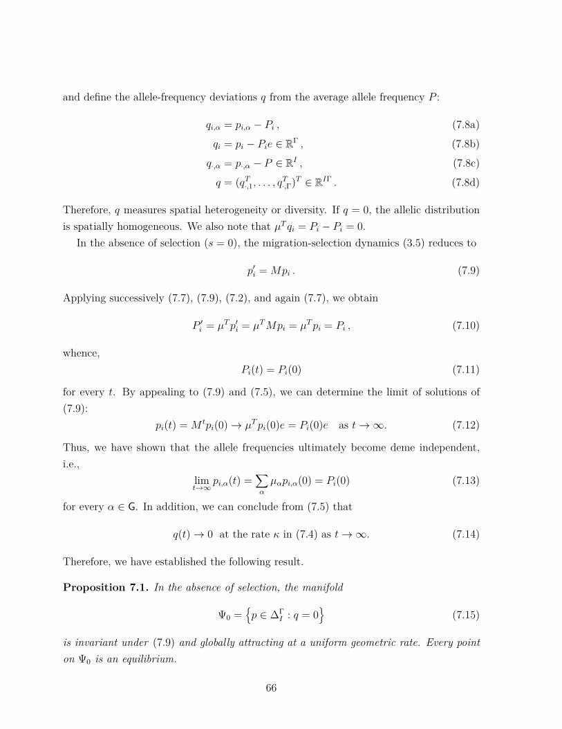
and define the allele-frequency deviations q from the average allele frequency P :

qi,α = pi,α − Pi , (7.8a)

qi = pi − Pie ∈ RΓ , (7.8b)

q·,α = p·,α − P ∈ RI , (7.8c)

q = (qT·,1, . . . , qT·,Γ)T ∈ RIΓ . (7.8d)

Therefore, q measures spatial heterogeneity or diversity. If q = 0, the allelic distributionis spatially homogeneous. We also note that µT qi = Pi − Pi = 0.

In the absence of selection (s = 0), the migration-selection dynamics (3.5) reduces to

p′i = Mpi . (7.9)

Applying successively (7.7), (7.9), (7.2), and again (7.7), we obtain

P ′i = µTp′i = µTMpi = µTpi = Pi , (7.10)

whence,Pi(t) = Pi(0) (7.11)

for every t. By appealing to (7.9) and (7.5), we can determine the limit of solutions of(7.9):

pi(t) = M tpi(0)→ µTpi(0)e = Pi(0)e as t→∞. (7.12)

Thus, we have shown that the allele frequencies ultimately become deme independent,i.e.,

limt→∞

pi,α(t) =∑α

µαpi,α(0) = Pi(0) (7.13)

for every α ∈ G. In addition, we can conclude from (7.5) that

q(t)→ 0 at the rate κ in (7.4) as t→∞. (7.14)

Therefore, we have established the following result.

Proposition 7.1. In the absence of selection, the manifold

Ψ0 =p ∈ ∆Γ

I : q = 0

(7.15)

is invariant under (7.9) and globally attracting at a uniform geometric rate. Every pointon Ψ0 is an equilibrium.

66

Remark 7.2. On the manifold Ψ0 there is no variation in allele frequencies among thedemes. Thus, at every equilibrium there is spatial uniformity. Within in each deme theequilibrium allele frequency is Pi(0), the spatially averaged initial frequency of Ai, i.e.,Pi(0) = ∑

α µαpi,α(0).

Remark 7.3. Proposition 7.1 does not hold if the migration matrix is reducible or peri-

odic. If, for instance, M =(

1 012

12

), then an allele that is initially absent in the second

deme will be also absent at equilibrium, whereas its frequency can be positive in the first

deme. If M =(

0 11 0

), then each generation the gamete frequencies are swapped between

the demes. In both cases, convergence to q = 0 will in general not occur.

Because in the absence of selection the dynamics is degenerate, regular perturbationmethods such as those leading to Theorem 6.4 cannot be applied. In a different context(weak selection in a panmictic multilocus model) Nagylaki et al. (1999) developed amethod to deal with certain nonsingular perturbations. It can be applied to the presentmodel with weak selection.

In the following, we analyze (3.5) in terms of (P, q) rather than p. We will need thefollowing average selection coefficients of AiAj, Ai, and the entire population:

ρij =∑α

µαrij,α , (7.16a)

ρi(P ) =∑j

ρijPj , (7.16b)

ρ(P ) =∑i,j

ρijPiPj . (7.16c)

We scale generations by the selection intensity,

t = bτ/sc , (7.17)

and call the differential equationdPidτ = Pi[ρi(P )− ρ(P )] , (7.18a)

q = 0 (7.18b)

on ∆ΓI the strong-migration limit, or the weak-selection limit, of (3.5). Of course, one

could also consider (7.18a) on ∆I . The differential equation (7.18a) has the same form asthe panmictic continuous-time single-locus dynamics (2.23). Because

dρ(P )dPi

= 2ρi(P ) , (7.19)

67

we obtaindρ(P )

dτ = 2∑i

Pi[ρi(P )− ρ(P )]2 ≥ 0 , (7.20)

and equality holds exactly at the equilibria of (7.18). In particular, the internal equilibriaare the critical points of ρ, and this is true for every subsystem. Hence, the strong-migration limit is gradient like (a so-called Svirezhev-Shashahani gradient).

We are now in the position to formulate the main theoretical result of this section.

Theorem 7.4 (Nagylaki and Lou 2007, Theorem 4.5). Suppose (7.1), the (ergodic) back-ward migration matrix M is fixed, s > 0 is sufficiently small, and that every equilibriumof (7.18a) is hyperbolic.

(a) The set of equilibria Ξ0 ⊂ ∆ΓI of (7.18) contains only isolated points, as does the

set of equilibria Ξs ⊂ ∆ΓI of (3.5). As s → 0, each equilibrium in Ξs converges to the

corresponding equilibrium in Ξ0.(b) In the neighborhood of each equilibrium in Ξ0, there exists exactly one equilibrium

point in Ξs. The stability of each equilibrium in Ξs is the same as that of the correspondingequilibrium in Ξ0; i.e., each pair is either asymptotically stable or unstable.

(c) Every solution p(t) of (3.5) converges to one of the equilibrium points in Ξs.

The essence of this theorem and its proof is that under strong migration (i) the exactdynamics quickly leads to spatial quasi-homogeneity. In fact, it can be shown that

q(t) = O(s) (7.21)

holds for every t ≥ t, where t = (− ln s)/κ and |λ1| < κ < 1; see (7.4). (ii) After thisevolutionary short time, the exact dynamics can be perceived as a perturbation of thestrong-migration (weak-selection) limit (7.18). The latter is much easier to study becauseit is formally equivalent to a panmictic single-locus selection dynamics.

The proof of Theorem 7.4 is much deeper than that of Theorem 6.4. Therefore, wepresent only a sketch.

Outline of the proof of Theorem 6.4. Proposition 7.1 and the theory of normally hyper-bolic manifolds imply that for sufficiently small s, there exists a smooth invariant manifoldΨs close to Ψ0, and Ψs is globally attracting for (3.5) at a geometric rate (see Nagylakiet al. 1999, and the references there). The manifold Ψs is characterized by an equation ofthe form

q = sψ(P, s) , (7.22)

68

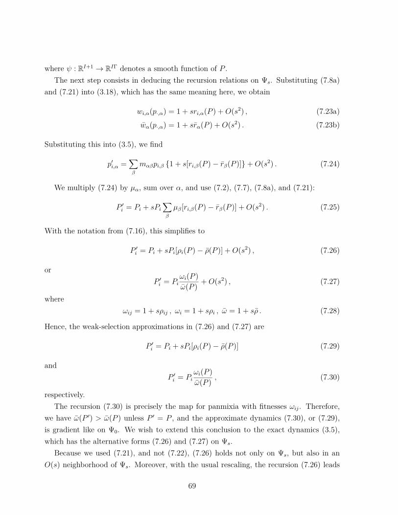
where ψ : RI+1 → RIΓ denotes a smooth function of P .The next step consists in deducing the recursion relations on Ψs. Substituting (7.8a)

and (7.21) into (3.18), which has the same meaning here, we obtain

wi,α(p·,α) = 1 + sri,α(P ) +O(s2) , (7.23a)

wα(p·,α) = 1 + srα(P ) +O(s2) . (7.23b)

Substituting this into (3.5), we find

p′i,α =∑β

mαβpi,β 1 + s[ri,β(P )− rβ(P )]+O(s2) . (7.24)

We multiply (7.24) by µα, sum over α, and use (7.2), (7.7), (7.8a), and (7.21):

P ′i = Pi + sPi∑β

µβ[ri,β(P )− rβ(P )] +O(s2) . (7.25)

With the notation from (7.16), this simplifies to

P ′i = Pi + sPi[ρi(P )− ρ(P )] +O(s2) , (7.26)

orP ′i = Pi

ωi(P )ω(P ) +O(s2) , (7.27)

whereωij = 1 + sρij , ωi = 1 + sρi , ω = 1 + sρ . (7.28)

Hence, the weak-selection approximations in (7.26) and (7.27) are

P ′i = Pi + sPi[ρi(P )− ρ(P )] (7.29)

andP ′i = Pi

ωi(P )ω(P ) , (7.30)

respectively.The recursion (7.30) is precisely the map for panmixia with fitnesses ωij. Therefore,

we have ω(P ′) > ω(P ) unless P ′ = P , and the approximate dynamics (7.30), or (7.29),is gradient like on Ψ0. We wish to extend this conclusion to the exact dynamics (3.5),which has the alternative forms (7.26) and (7.27) on Ψs.

Because we used (7.21), and not (7.22), (7.26) holds not only on Ψs, but also in anO(s) neighborhood of Ψs. Moreover, with the usual rescaling, the recursion (7.26) leads

69

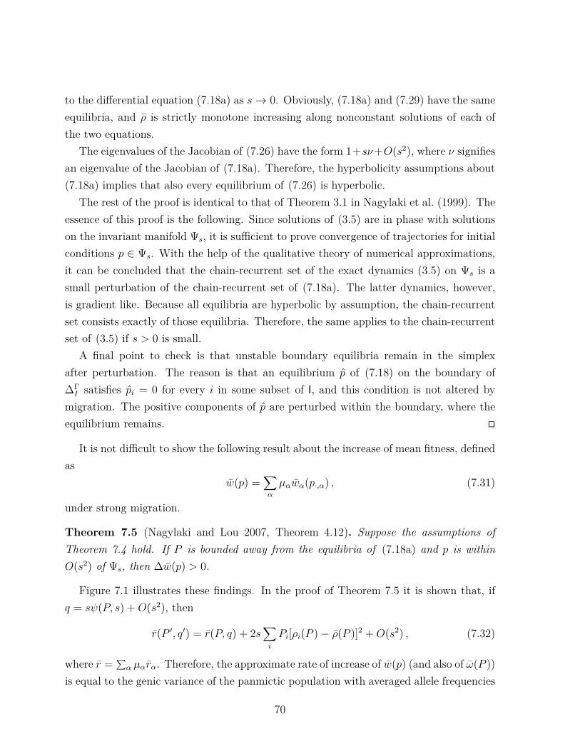
to the differential equation (7.18a) as s→ 0. Obviously, (7.18a) and (7.29) have the sameequilibria, and ρ is strictly monotone increasing along nonconstant solutions of each ofthe two equations.

The eigenvalues of the Jacobian of (7.26) have the form 1+sν+O(s2), where ν signifiesan eigenvalue of the Jacobian of (7.18a). Therefore, the hyperbolicity assumptions about(7.18a) implies that also every equilibrium of (7.26) is hyperbolic.

The rest of the proof is identical to that of Theorem 3.1 in Nagylaki et al. (1999). Theessence of this proof is the following. Since solutions of (3.5) are in phase with solutionson the invariant manifold Ψs, it is sufficient to prove convergence of trajectories for initialconditions p ∈ Ψs. With the help of the qualitative theory of numerical approximations,it can be concluded that the chain-recurrent set of the exact dynamics (3.5) on Ψs is asmall perturbation of the chain-recurrent set of (7.18a). The latter dynamics, however,is gradient like. Because all equilibria are hyperbolic by assumption, the chain-recurrentset consists exactly of those equilibria. Therefore, the same applies to the chain-recurrentset of (3.5) if s > 0 is small.

A final point to check is that unstable boundary equilibria remain in the simplexafter perturbation. The reason is that an equilibrium p of (7.18) on the boundary of∆ΓI satisfies pi = 0 for every i in some subset of I, and this condition is not altered by

migration. The positive components of p are perturbed within the boundary, where theequilibrium remains.

It is not difficult to show the following result about the increase of mean fitness, definedas

w(p) =∑α

µαwα(p·,α) , (7.31)

under strong migration.

Theorem 7.5 (Nagylaki and Lou 2007, Theorem 4.12). Suppose the assumptions ofTheorem 7.4 hold. If P is bounded away from the equilibria of (7.18a) and p is withinO(s2) of Ψs, then ∆w(p) > 0.

Figure 7.1 illustrates these findings. In the proof of Theorem 7.5 it is shown that, ifq = sψ(P, s) +O(s2), then

r(P ′, q′) = r(P, q) + 2s∑i

Pi[ρi(P )− ρ(P )]2 +O(s2) , (7.32)

where r = ∑α µαrα. Therefore, the approximate rate of increase of w(p) (and also of ω(P ))

is equal to the genic variance of the panmictic population with averaged allele frequencies

70

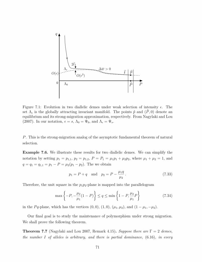
0

Fig. 1

P

q

Λε

Λ0

O(ε)

O(ε2)

∆w > 0

2t

t

p

P

1

P

q

Λε

Λ0

O(ε)

O(ε2)

∆w > 0

2t

t

p

P

1

P

q

Λε

Λ0

O(ε)

O(ε2)

∆w > 0

2t

t

p

P

1

P

q

Λε

Λ0

O(ε)

O(ε2)

∆w > 0

2t

t

p

P

1

P

q

Λε

Λ0

O(ε)

O(ε2)

∆w > 0

2t

t

p

P

1

P

q

Λε

Λ0

O(ε)

O(ε2)

∆w > 0

2t

t

p

P

1

P

q

Λε

Λ0

O(ε)

O(ε2)

∆w > 0

2t

t

p

P

1

P

q

Λε

Λ0

O(ε)

O(ε2)

∆w > 0

2t

t

p

P

1

P

q

Λε

Λ0

O(ε)

O(ε2)

∆w > 0

2t

t

p

P

1

P

q

Λε

Λ0

O(ε)

O(ε2)

∆w > 0

2t

t

p

P

1

P

q

Λε

Λ0

O(ε)

O(ε2)

∆w > 0

2t

t

p

P

1

Figure 7.1: Evolution in two diallelic demes under weak selection of intensity ε. Theset Λε is the globally attracting invariant manifold. The points p and (P , 0) denote anequilibrium and its strong-migration approximation, respectively. From Nagylaki and Lou(2007). In our notation, ε = s, Λ0 = Ψ0, and Λε = Ψs.

P . This is the strong-migration analog of the asymptotic fundamental theorem of naturalselection.

Example 7.6. We illustrate these results for two diallelic demes. We can simplify thenotation by setting p1 = p1,1, p2 = p1,2, P = P1 = µ1p1 + µ2p2, where µ1 + µ2 = 1, andq = q1 = q1,1 = p1 − P = µ2(p1 − p2). The we obtain

p1 = P + q and p2 = P − µ1q

µ2. (7.33)

Therefore, the unit square in the p1p2-plane is mapped into the parallelogram

max−P,−µ2

µ1(1− P )

≤ q ≤ min

1− P, µ2

µ1P

(7.34)

in the Pq-plane, which has the vertices (0, 0), (1, 0), (µ1, µ2), and (1− µ1,−µ2).

Our final goal is to study the maintenance of polymorphism under strong migration.We shall prove the following theorem.

Theorem 7.7 (Nagylaki and Lou 2007, Remark 4.15). Suppose there are Γ = 2 demes,the number I of alleles is arbitrary, and there is partial dominance, (6.16), in every

71

deme. Then there exists an open set of migration and selection parameters such thatglobal convergence to an internal equilibrium point occurs. Thus, arbitrarily many allelescan be maintained at equilibrium.

Thus, in contrast to ‘common believe’, ‘more’ polymorphism can be maintained understrong migration than under weak migration. However, the sufficient conditions given inthe proof become very stringent as the number of alleles increases above two.

Proof. We choose the backward migration matrix

M =(

1−m1 m1m2 1−m2

), (7.35)

where 0 < m1,m2 < 1, so that M is ergodic. It has the maximal left eigenvector µ =( m2m1+m2

, m1m1+m2

)T . We assume that the selection coefficients rij,α in (7.1) satisfy

rii,1 < rij,1 < rjj,1 , (7.36a)

rij,2 = −m2

m1rij,1 , (7.36b)

rii,2 < −m2

m1rii,1 , (7.36c)

−m2

m1rij,1 < rii,2 (7.36d)

for every n, every i and every j > i. Choosing selection coefficients in the order rii,1,rij,1, rij,2, rii,2 shows that (7.36) can be satisfied. By (7.36a), there is partialdominance in deme 1. That partial dominance also holds in deme 2 follows by apply-ing successively (7.36c) with j instead of i, (7.36a), (7.36b), again (7.36b), and (7.36d).Equations (7.36b) and (7.36c) show that

ρij =2∑

α=1µαrij,α = 0 and ρii < 0 , (7.37)

respectively, for every i, j such that i , j. Therefore, in the strong-migration limit (7.18)a unique internal equilibrium exists. It is given by

Pi = 1ρii

/∑j

1ρjj

. (7.38)

Global convergence to this equilibrium occurs because ρ(P ) = ∑i,j ρijPiPj is strictly

increasing along trajectories except at equilibria and, by (7.37), ρ(P ) is strictly concave

72

on ∆I . It is not difficult to show that (7.38) is hyperbolic. Therefore, Theorem 7.4 impliesglobal asymptotic stability of an internal equilibrium under sufficiently weak selection.The internal equilibrium (7.38) of (7.18) will persist under small perturbations of theparameters (rij,α), as will the perturbed equilibrium under strong migration. Therefore,a globally asymptotically stable and fully polymorphic equilibrium exists for an open setof parameters.

Remark 7.8. The inequalities in (7.36) imply the presence of dominance. Suppose thereis no dominance in deme 1, i.e.,

rij,1 = 12(rii,1 + rjj,1) . (7.39)

Then we obtain from (7.36)

rij,2 = −12m2

m1(rii,1 + rjj,1) > 1

2(rii,2 + rjj,2) , (7.40)

which proves dominance in deme 2.

Remark 7.9. The proof of Theorem 7.7 applies in the Levene case when m1 + m2 = 1.Thus, the theorem holds for the Levene model.

Remark 7.10. If there is DIDID in every deme, then it can be shown that, generically,there exists a globally asymptotically stable monomorphic equilibrium. Thus, no poly-morphism at all is maintained. This follows by applying an argument similar to that inProposition 6.6 to the strong-migration limit and then extending to strong migration.

8 Derivation of the PDE migration-selection model

Our aim is the motivation and derivation of a model that describes dispersal of individualsor alleles in continuous space. The most common approach is to model dispersal bydiffusion in space (Fisher 1937, Kolmogorov et al. 1937, Haldane 1948; see Nagylaki andLou 2008 for a recent review). This is appropriate if the dispersal distance is typicallysmall relative to changes in the environment. In this section we demonstrate how the wellknown partial differential equation can be obtained as an approximation to the discrete-time discrete-demes model. The derivation outlined below is inspired by the more generalones given by Nagylaki (1989, 1996).

The starting point is the model derived in Section 3. Here, it will be convenient to usethe number Nα of individuals in deme α instead of the deme proportions cα. Then (3.8)

73

becomesmβα = N∗αmαβ∑

γ N∗γ mγβ

. (8.1)

Using (8.1), we can rewrite (3.5a) as(∑γ

N∗γ mγα

)p′i,α =

∑β

N∗βmβαp∗i,β , (8.2a)

wherep∗i,β = pi,β

wi,βwβ

. (8.2b)

We measure time, t, in generations and suppose that wij,α(pα, t), mαβ(t), and Nα(t)are given for every i, j, α, β, t, and that N∗α = N∗α(Nα, pα, t), where pα = (p1,α, . . . , pI,α)>.Then (8.2) describes the model completely.

We treat only the one-dimensional case and assume that demes are arranged in alinear array. Examples include organisms confined to a river, riverbank, seashore, ormountain range. The model applies to populations in two-dimensional habitats if onlyone coordinate, such as latitude, altitude on a mountain range, or distance from a riveror seashore matter.

We scale space and time as follows:

x = εα, y = εβ, t = bτ/λc. (8.3)

In the new units, ε is a measure of distance between adjacent colonies and λ correspondsto the length of one generation. We let

ε→ 0 and λ→ 0 such that ε2

λremains fixed. (8.4)

We suppose that there are numbers rij,α(pα, t) ∈ [−1, 1] such that

wij,α(pα, t) = 1 + λrij,α(pα, t) (8.5)

holds for every i, j, α, and t. Therefore, we obtain from (8.2b)

p∗i,α = pi,α + λsi,α(pα, t) + o(λ) (8.6)

because wi,α/wα = 1 + λ(ri,α − rα) + o(λ) and si,α = pi,α(ri,α − rα).In terms of the scaled variables x, y and τ , we write

Nα(t) = ρ(x, τ), pi,α(t) = πi(x, τ), si,α(pα, t) = Si(π, x, τ). (8.7)

74

Here and below, we assume that all quantities marked with a caret (ˆ) have uniform andcontinuous limits in x as λ → 0. We omit the carets in this limit. Thus, our aim isto derive the system of PDEs that the πi(x, τ) have to satisfy if they are theλ→ 0 limit of the solution pα(t) of (8.2).

Doing this in an exact mathematical way is a formidable task because the frequencydistributions pi,α(t) live on the discrete set Γ, whereas the πi(x, τ) live on R. Therefore, anapproximation requires an embedding into an appropriate Banach space of measures andconvergence will be interpreted in the weak∗ sense. Therefore, in the formal derivation,test functions are used. A key role below is played by the diffusion hypothesis (8.10), whichguarantees that dispersal in the real line has the same mean and variance as the dispersalof the embedded discrete-demes model. Higher moments of the dispersal distribution areneglected, i.e., assumed to vanish. The idea of the formal derivation given below is closelyrelated to that of deriving a diffusion approximation for a (sequence of) Markov chain(s)(e.g., Ewens 1979, Chap. 4.2). For the much deeper proof of convergence of solutions, seeEthier and Kurtz (1986, Chap. 7.4).

Our assumptions imply that (8.6) holds uniformly in x for every τ , i.e.,

limλ→0

supx

∣∣∣∣∣ π∗i (x, τ)− πi(x, τ)λ

− Si(π, x, τ)∣∣∣∣∣ = 0 (8.8)

or, simply,π∗i (x, τ) = πi(x, τ) + λSi(π, x, τ) + o(λ) (8.9)

uniformly in x as λ→ 0, where the superscript ∗ again denotes frequencies after selection.Because we want to model migration by diffusion we require the following diffusion

hypothesis (cf. Feller 1971, p. 333):

limλ→0

ε

λ

∑β:|α−β|<θ/ε

(β − α)mαβ(t) = M(x, τ), (8.10a)

limλ→0

ε2

λ

∑β:|α−β|<θ/ε

(β − α)2mαβ(t) = V (x, τ), (8.10b)

limλ→0

1λ

∑β:|α−β|≥θ/ε

mαβ = 0, (8.10c)

uniformly in x and for every θ > 0. Here, M and V represent the mean and varianceof displacement by dispersal per new time unit in new length units. The correspondingquantities in generations are λM and λV , respectively. We note that in the limit λ→ 0the variance of migrational displacement equals its mean square. We assume that the

75

partial derivatives that appear below are the uniform limits as λ→ 0 of the correspondingdiscrete quantities and are continuous.

Formidable algebra (see subsection 8.1) yields the PDE7

πi,τ = 12V (y, τ)πi,yy −M(y, τ)πi,y + 1

ρ(y, τ)((ρ(y, τ)V (y, τ))yπi,y

)+ Si(π, y, τ), (8.11)

which we rewrite as

pi,t = 12V pi,xx +

[ρ−1(ρV )x −M

]pi,x + Si, (8.12)

where we suppressed the dependence of M , V , and ρ on x and t, and that of Si on p, x,and t. We assume (8.12) holds on a (spatial) domain Ω that is a bounded or unboundedopen interval. For extensions to more than one space dimension, we refer to Nagylakiand Lou (2008). In general, (8.12) is a complicated PDE, not simply a reaction-diffusionequation.

In the important special case in which ρ = const. and migration is homogeneous andisotropic, so that M = 0 and V = σ2 (a positive constant), (8.12) simplifies to

pi,t = 12σ

2pi,xx + Si. (8.13a)

This is the form most frequently studied in the literature. Usually, we assume that

Si = Si(p, x) = pi(x, t)[ri(x)− r(x)], (8.13b)

where ri(x) = ∑j rij(x)pj(x, t) and r(x) = ∑

ij rij(x)pi(x, t)pj(x, t); cf. (8.5) – (8.7) andChapter 2. In addition, we always assume

pi(x, 0) ≥ 0, pi(x, 0) . 0,∑j

pj(x, 0) ≡ 1 for every x ∈ Ω, (8.13c)

as well as the boundary condition

pi,x(b, t) = 0 for every i and t > 0, (8.13d)

which is assumed to hold at every endpoint b of the spatial domain Ω. Thus, equations(8.13a), (8.13b), (8.13c), and (8.13d) constitute our basic model.

7We denote first and second partial derivatives of a function F (x, z) with respect to x by Fx and Fxxrespectively.

76

8.1 ∗Formal derivation of (8.11)

In view of (8.5) we assume that

N∗α = Nα(1 +O(λ)), (8.14)

which includes both soft and hard selection; cf. (3.19).For a bounded function fα(t) = F (x, τ), such that Fxx is twice continuously differen-

tiable, the diffusion hypothesis (8.10) together with Taylor’s theorem imply

∑α

mβαfα(t) = F (y, τ) + λM(y, τ)Fy(y, τ) + 12λV (y, τ)Fyy(y, τ) + o(λ) (8.15)

uniformly as λ→ 0.[Proof: We decompose

∑α

mβαfα =∑

α:|β−α|< θε

mβαfα +∑

α:|β−α|≥ θε

mβαfα,

where ∑α:|β−α|≥ θεmβαfα = o(λ) by (8.10c) because F is bounded. To approximate the

first term, we use first Taylor expansion of fα = F (x), then (8.10):

∑α:|β−α|< θ

ε

mβαfα =∑

α:|β−α|< θε

mβα

(F (y) + (y − x)Fy(y) + 1

2(y − x)2Fyy(y) + o((y − x)2))

=

∑α:|β−α|< θ

ε

mβα

F (y) +

∑α:|β−α|< θ

ε

mβαε(β − α)

Fy(y)

+ 12

∑α:|β−α|< θ

ε

mβαε2(β − α)2

Fyy(y) + o((y − x)2)

= F (y) (1 + o(λ)) + λ(M(y) + o(1))Fy(y) + λ

2 (V (y) + o(1))Fyy(y) + o(ε2),

which yields (8.15). ]Now we choose test functions φα(t) = Φ(x, τ) such that Φ, Φx, and Φxx are continuous

and vanish outside of the interval (x1, x2), where x1 < x2 are arbitrary but fixed. Wemultiply the discrete recursion (8.2) by φα and sum over all α:

∑α,β

N∗βmβαp′

i,αφα =∑α,β

N∗βmβαp∗i,βφα. (8.16)

77

Using first (8.6) and (8.15), then (8.7), we obtain for the right hand side of (8.16)∑β

N∗βp∗i,β

∑α

mβαφα

=∑β

N∗β (pi,β + λsi,β + o(λ))(

Φ(y) + λM(y, τ)Φy(y) + 12λV (y, τ)Φyy(y) + o(λ)

)=∑β

N∗β[πi(y, τ)Φ(y) + λSi(π, y, τ)Φ(y)

+ λM(y, τ)Φy(y)πi(y, τ) + 12λV (y, τ)Φyy(y)πi(y, τ) + o(λ)

]. (8.17)

Using p′i,α = πi(x, τ) + λπi,τ (x, τ) + o(λ) and (8.15), we obtain for the left hand side of

(8.16) in essentially the same way as above:∑α,β

N∗βmβαp′i,αφα

=∑β

N∗β[πi(y, τ)Φ(y) + λπi,τ (y, τ)Φ(y) + λM(y, τ) [πi(y, τ)Φ(y)]y

+ 12λV (y, τ) [πi(y, τ)Φ(y)]yy + o(λ)

]. (8.18)

Equating (8.17) and (8.18), we get

∑β

N∗β

[λΦ(y)

(πi,τ (y, τ)− Si(π, y, τ) +M(y, τ)πi,y(y) + 1

2V (y, τ)πi,yy(y, τ))

+ λV (y, τ)πi,y(y, τ)Φy(y) + o(λ)]

= 0.

If we take the limit λ→ 0, the left side converges to the integral∫ x2

x1

[ρ(y, τ)

(πi,τ (y, τ)− Si(π, y, τ) +M(y, τ)πi,y(y, τ) + 1

2V (y, τ)πi,yy(y, τ))−

−(ρ(y, τ)V (y, τ)πi,y(y, τ)

)y

]Φ(y)dy = 0, (8.19)

where we have used that N∗β = Nβ(1 + O(λ)) → ρ(y, τ) as λ → 0 (8.7), and V (y)πi,yΦy

was integrated by parts. Since Φ is arbitrary, the term in brackets must vanish for ally ∈ (x1, x2) if we assume ρ(y, τ) > 0 for all y and ρ.

Therefore, after performing the differentiation (ρV πi,y)y = (ρV )yπi,y + ρV πi,yy, weobtain the PDE

πi,τ = 12V (y, τ)πi,yy −M(y, τ)πi,y + 1

ρ(y, τ)((ρ(y, τ)V (y, τ))yπi,y

)+ Si(π, y, τ) ,

78

i.e., (8.11).It remains to derive the boundary condition (8.13d). It follows from the condition that

at the boundary, there is no flux of individuals or of alleles. Let us assume, for instance,that the habitat is [0,∞), with no migration left of the origin. We start with a discretemodel, and consider colonies 0, 1, 2, . . .. We assume m0α = 0 if α > Γ. Inserting (8.5)into the recursion, we obtain

p′i,0 =Γ∑α=0

m0αpi,α +O(λ)

as λ→ 0. A simple calculation yields

λ

ε

p′i,0 − pi,0λ

=Γ∑α=0

m0αpi,α − pi,0

ε+O(ε). (8.20)

Letting λ→ 0, we obtain (p′i,0 − pi,0)/λ = (πi(0, τ + λ)− πi(0, τ))/λ→ πi,τ (0, τ), whencethe left-hand side of (8.20) converges to zero. Similarly, letting λ→ 0, we obtain (pi,α −pi,0)/ε = (πi(εα, τ) − πi(ε0, τ))/ε → απi,x(0, τ). Therefore, the right-hand side of (8.20)converges to πi,x(0, τ)∑Γ

α=0 αm0α, from which we conclude that the boundary conditionis pi,x(0, t) = 0 for every i and t.

8.2 Existence and uniqueness of solutions of (8.12)

We conclude with results concerning existence and uniqueness of solutions.

Remark 8.1. Holder continuity. A function f : R→ R is Holder continuous if there existconstants c and α ∈ (0, 1], such that

|f(x)− f(y)| ≤ c|x− y|α

for every x, y in the domain of f . A Holder continuous function is uniformly continuous;if α = 1, then it is Lipschitz continuous.

Denote by C(Ω) the continuous real-valued functions on Ω, by

Ck(Ω) = u : Dmu ∈ C(Ω), 0 ≤ m ≤ k ,

and by Ck(Ω) those functions in Ck(Ω) with the property that Dmu has a continuousextension to Ω, for each m with 0 ≤ m ≤ k. Finally, denote by Ck,α(Ω) those u ∈ Ck(Ω)that have the property that Dku is Holder continuous with exponent α.

79

Then Ck(Ω) and Ck,α(Ω) are separable Banach spaces with the norms

‖u‖Ck = max0≤m≤k

supx∈Ω|Dmu(x)|

and‖u‖Ck,α = ‖u‖Ck + sup

x,y∈Ω,x,y

|Dαu(x)−Dαu(y)||x− y|α

,

respectively (Friedman 1969).

We assume that ρ(x), M(x), V (x), and rij(x) are all Holder continuous and pi(x, 0)is continuous on Ω. Then the standard existence theory of evolution equations (e.g.,Sell and You 2002) shows that the problem (8.13), or the more general version in which(8.13a) is replaced by (8.12), has a unique classical solution p(x, t) that exists for all time,pi ∈ C(Ω× [0,∞))∩C2,1(Ω× (0,∞)) and pi(x, t) ≥ 0 for every i, every x ∈ Ω, and everyt > 0. Therefore, without loss of generality, we posit that 0 < pi(x, 0) < 1 for every i andevery x ∈ Ω.

Finally, we show that 0 < pi(x, t) < 1 holds for all i, x, and t > 0, and ∑i pi(x, t) ≡ 1for every x ∈ Ω and t > 0. By summation, we obtain from (8.13a)

∂

∂t

(∑i

pi

)= σ2

2∂2

∂x2

(∑i

pi

)+ λr

[1−

(∑i

pi

)], (8.21)

from (8.13c) ∑i

pi(x, 0) ≡ 1, (8.22)

and from (8.13d)∂

∂x

(∑i

pi

)(b, t) = 0. (8.23)

By the uniqueness of the solutions of linear parabolic equations (e.g., Friedman 1969), weobtain ∑

i pi(x, t) ≡ 1 for every x ∈ Ω and every t > 0. By the maximum principle forparabolic equations (Appendix C or Protter and Weinberger 1984), if pi(x, 0) . 0, thenpi(x, t) > 0 for every x ∈ Ω and t > 0. Hence, without loss of generality, we assume thatpi(x, t) > 0 for every i, x ∈ Ω, and t ≥ 0.

9 PDE models for two alleles

The majority of available theory about the PDE migration-selection model assumes twoalleles per locus. In this section, we shall treat two classical scenarios: Fisher waves

80

and clines caused by spatial inhomogeneity. Because we assume only two alleles, thenotation can be simplified. Instead of using the vector (p1, p2)>, it is sufficient to usep(x, t) = p1(x, t). In addition, we set S(x, p) = S1((p1, p2)>, x). The models studiedbelow are special cases of the PDE

∂p

∂t= ∆p+ S(x, p) in Ω× (0,∞) (9.1a)

subject to the initial condition

0 ≤ p(x, 0) ≤ 1 , p(x, 0) . 0 , p(x, 0) . 1 on Ω . (9.1b)

Here, ∆f = ∑nj=1

∂2f∂x2j

denotes the Laplace operator (in most of our calculations, we assumen = 1, but the theory in Sect. 9.2 is more general). In addition, we will assume that S(x, p)can be factored into the form

S(x, p) = sg(x)f(p) , (9.2)

which is possible in important special cases, as outlined below. Appropriate boundaryconditions will be imposed in the various special cases.

We will factor out the selection intensity s, i.e., we assume that the fitness of AiAj issrij(x), and rij is independent of p and t. Then we obtain

S(x, p) = sp(r1(x, p)− r(x, p))

= sp(1− p)(r12(x)− r22(x) + [r11(x)− 2r12(x) + r22(x)]p

). (9.3)

Inn the following important special cases the factorization (9.2) is obtained.a) No dominance: rij(x) = vi(x) + vj(x) on Ω. Then

S(x, p) = s[v1(x)− v2(x)]p(1− p). (9.4)

b) A1 is dominant: r11(x) = r12(x) on Ω. Then

S(x, p) = s[r11(x)− r22(x)]p(1− p)2. (9.5)

c) A1 is recessive: r22(x) = r12(x) on Ω. Then

S(x, p) = s[r11(x)− r22(x)]p2(1− p). (9.6)

d) All selection coefficients have the same spatial dependence g(x). Then we can choose

r11(x) = g(x), r12(x) = hg(x), r22(x) = −g(x), (9.7)

where h signifies the degree of dominance, and obtain

S(x, p) = sg(x)p(1− p)(1 + h− 2hp); (9.8)

cf. (2.15). Note that h = 0, 1,−1 yields the cases a), b), c), respectively.

81

9.1 Fisher’s equation

This model was introduced independently by Fisher (1937) and Kolmogorov et al. (1937).It assumes that fitnesses are independent of the spatial position and exhibit no dominance.Fisher envisaged to model the spread of a mutant that has a constant fitness advantageover the wild type. These assumptions together with (9.4) show that (8.13a) becomes

pt = 12σ

2pxx + sp(1− p), (9.9)

where x ∈ Ω = (−∞,∞). By rescaling time and space according to τ = st and y =x√

2s/σ2, (9.9) simplifies topt = pxx + p(1− p). (9.10)

Fisher wanted to find out how fast a new favorable mutant spreads through a spatiallydistributed population.

It turns out that the (biologically relevant) solutions are “wave like”. In general, PDEscan have quite different kinds of wave-like solutions. We shall be mainly concerned withwave fronts. They have the following properties:

0 ≤ u ≤ 1, u(−∞) = 1, and u(∞) = 0. (9.11)

(One can also assume u(−∞) = 0 and u(∞) = 1. Then the wave front will travel in theopposite direction.) A solitary wave (soliton, pulse) satisfies

u ≥ 0, u , 0, u(−∞) = u(∞) = 0. (9.12)

To find wave-front solutions of (9.10), we set

p(x, t) = u(x− ct). (9.13)

Then (9.10) becomes −cu′(x− ct) = u′′(x− ct) + u(x− ct)[1− u(x− ct)], i.e.,

u′′ + cu′ + u(1− u) = 0. (9.14)

Here, u′ indicates differentiation with respect to the (single) variable on which u depends.If we introduce v = u′, then (9.14) can be written as the following system of linear ODEs:

u′ = v,

v′ = −cv − u(1− u).(9.15)

82

We study the system (9.15). The equilibria are (0, 0) and (1, 0). A wave front corre-sponds to a heteroclinic orbit joining these two equilibria and satisfying 0 ≤ u ≤ 1. TheJacobian of (9.15) is

J =(

0 1−1 + 2u −c

). (9.16)

Therefore, the Jacobians at the two equilibria are

J(0,0) =(

0 1−1 −c

)and J(1,0) =

(0 11 −c

). (9.17)

We find that the eigenvalues at (0, 0) are −12c±

12

√c2 − 4. Therefore, (0, 0) is asymp-

totically stable if and only if c > 0, and it is a nodal sink if and only if c ≥ 2. Theeigenvalues at (1, 0) are −1

2c ±12

√c2 + 4. Therefore, (1, 0) is always a saddle. The case

c < 0 is without interest because then both equilibria are unstable and a connecting, i.e.,heteroclinic, orbit is repelling. Therefore, we focus on the case c > 0. If 0 < c < 2, theheteroclinic orbit spirals. Therefore, it is not positive everywhere. Because the eigenvec-tors corresponding to the two eigenvalues are (c+

√c2 + 4, 2) and (c−

√c2 + 4, 2), we can

draw the phase portrait (see Figure 9.1). (Also note that v′ < 0 if v = 0 and 0 ≤ u ≤ 1,and v′ > 0 if v < −u(1− u)/c.)

A wave front exists if and only if c ≥ 2. For every c > 2, there exists a unique wavefront (Kolmogorov et al. 1937; Aronson and Weinberger 1975, 1978). The reason is thatthen one of the branches of the unstable manifold of (1, 0) must connect to (0, 0). Becausethe heteroclinic orbit satisfies v < 0 if 0 < u < 1, we have u′ = v < 0. Hence, the wavefront is strictly monotone decreasing. The point of inflection is given by u′′ = v′ = 0, i.e.,it satisfies v = −u(1− u)/c. In advance of this point, u′′ > 0.

An explicit wave-front solution of (9.10) is known for c = ±5/√

6 ≈ ±2.0412 (Ablowitzand Zeppetella, 1979):

u(z) =(1− rez/

√6)−2

, (9.18)

where r < 0 is arbitrary (Figure 9.2). Of course, if z → u(z) is a solution, then alsoz → u(z + a) for every a.

Kolmogorov et al. (1937) proved that the initial datum p(x, 0) = 1 if x < 0, andp(x, 0) = 0 if x > 0 converges to a wave with speed c = 2. McKean (1975) extended thisresult to initial data that converge sufficiently rapidly to 1 or 0 as x → −∞ or x → ∞,respectively. In addition, he proved that if for given c > 2, the initial function converges to1 at an appropriate (exponential) rate as x→ −∞, the corresponding solution convergesto a wave front with speed c. Thus, wave fronts are stable. For the original equation(9.9), the condition c > 2 transforms into c >

√2sσ2.

83

Figure 9.1: Phase portrait of (9.15) for c = 2.5.

-15 -10 -5 5 10 15x

0.2

0.4

0.6

0.8

1.0

u

Figure 9.2: The explicit wave-front solution (9.18) with r = −12 and c = 5/

√6.

84

Of course, it is unnatural that the speed is indeterminate. The reason is that diffusion(with a constant) rate can be expected to approximate biological reality only if sufficientlymany individuals of both types are present. Clearly, this is not the case at the extremefront or back of the wave. Therefore, in sufficiently large populations the wave speedshould be close to the minimum possible value of c = 2. Finally, initial data satisfyingp(x, 0)→ 0 as x→ ±∞ may converge to double waves.

There exist other types of simple solutions of (9.9). For instance,

p(x, t) = aest

1− a+ aest(9.19)

is a family of solutions that is constant in x and p(x, 0) ≡ a.

9.2 Clines under spatially heterogeneous selection

If genotypic fitnesses vary in space, then equilibrium allele frequencies can be expected tovary, too. One says a cline (in allele frequencies) occurs if the allele frequencies dependmonotonically on the spatial variable. Such patterns are frequently observed in spatiallydistributed populations if there is an environmental gradient, for a instance in tempera-ture. The first model of a cline is due to Haldane (1948), who motivated his study by theproblem of measuring selection in the deer mouse. Further important early theoreticalwork includes Fisher (1950), Slatkin (1973), Fleming (1975), and Nagylaki (1975).

First, we investigate a classical example; then we will turn to the general theory.

9.2.1 The step environment in the infinite cline

We assume Ω = (−∞,∞),pt = 1

2σ2pxx + sg(x)f(p), (9.20)

where f(p) = p(1− p)(1 + h− 2hp),

g(x) =

1 if x ≥ 0,−a if x < 0,

(9.21)

and a > 0; cf. (9.8). Of course, we are only interested in solutions satisfying 0 ≤ p(x, t) ≤ 1for all x and t.

If a stationary solution (a cline) exists, it must satisfy

p′′ + λf(p) = 0 if x ≥ 0, (9.22a)

p′′ − aλf(p) = 0 if x < 0, (9.22b)

85

where λ = 2s/σ2. Slatkin (1973) called√

2/λ = σ/√s the critical length of the cline.

We require the conditions

p′(∞) = p′(−∞) = 0, (9.23a)

p and p′ are continuous at x = 0. (9.23b)

Obviously, p ≡ 0 and p ≡ 1 are always solutions.Now suppose that there is no dominance, i.e., h = 0. Then f(p) = p(1 − p) and the

following solution of (9.22a) exists and is unique with respect to the above conditions (cf.Haldane 1948, Slatkin 1973, Nagylaki 1976):

p(x) = −12 + 3

2 tanh2

√λ2 x+ tanh−1

√1 + 2b

3

if x ≥ 0, (9.24a)

p(x) = 32 −

32 tanh2

√aλ2 x− tanh−1

√1− 2b

3

if x < 0, (9.24b)

where b = p(0) is the unique solution in (0, 1) of

(1 + a)(3b2 − 2b3) = 1. (9.25)

The solution (9.24) satisfies (9.23a), (9.23b), limx→∞ p(x) = 1, limx→−∞ p(x) = 0, and

p′(0) = b√

3− 2b√aλ

3 =√

aλ

3(1 + a) , (9.26)

where the last equality follows from (9.25). The second derivative at x = 0 is not contin-uous because p′′(0+) = −b(1− b)λ, whereas p′′(0−) = ab(1− b)λ.

Proof. We set ϕ(x, p) = p′(x). Then p′′ = ∂ϕ∂x

= ∂ϕ∂p

∂p∂x

= ∂ϕ∂pϕ. Therefore, (9.22a) can

be written as ∂ϕ∂pϕ = −λp(1 − p). Separating variables and integrating, we obtain ϕ2 =

C − 2λ(p2/2 − p3/3). Because ϕ(x, p) → 0 as x → ∞ (and p(x) → 1 as x → ∞), weobtain C = λ/3. Therefore, we have to solve(

dp

dx

)2

= λ

3 (1− p)2(1 + 2p). (9.27)

Separation of variables and integration yields (9.24a) if p(0) = b. Analogously, (9.22b)can be written as ∂ϕ

∂pϕ = aλp(1− p), from which we obtain

(dp

dx

)2

= aλ

3 p2(3− 2p). (9.28)

86

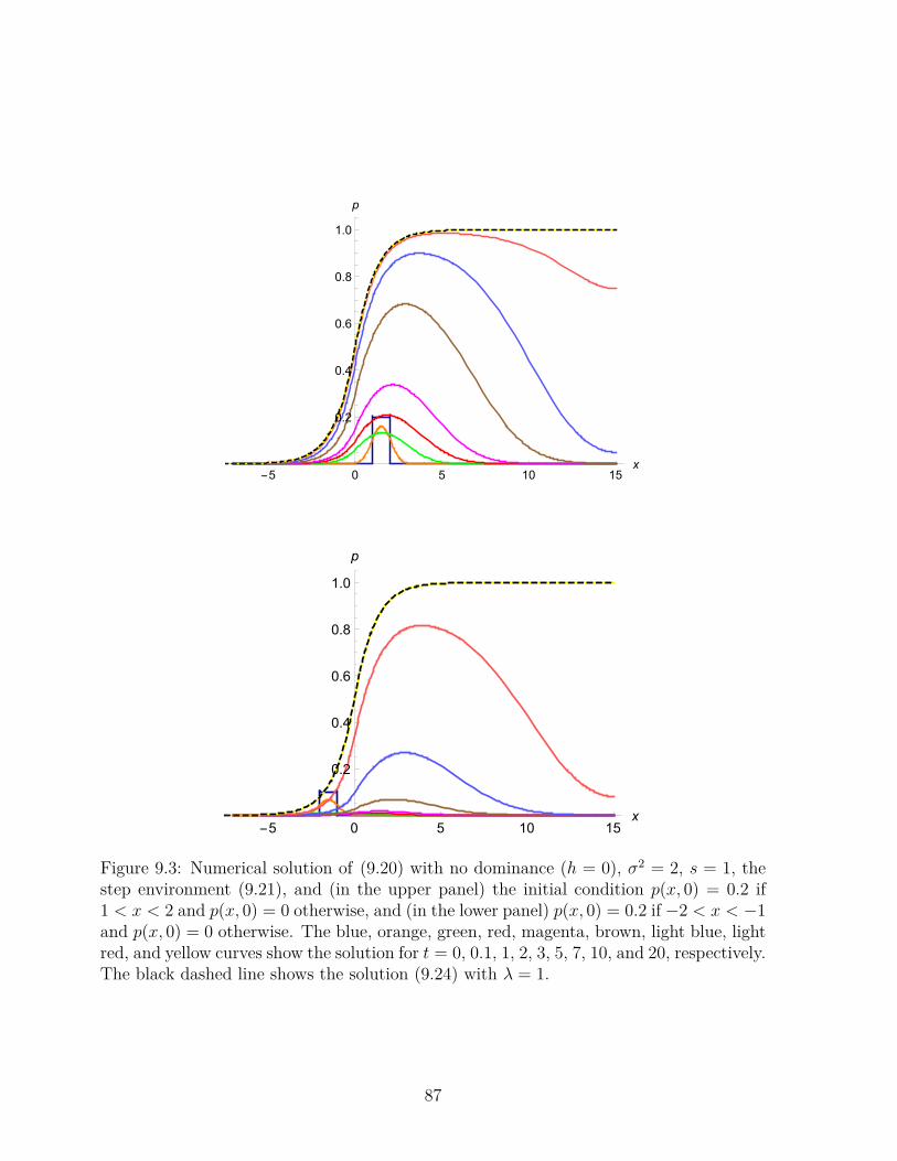
-5 0 5 10 15x

0.2

0.4

0.6

0.8

1.0

p

-5 0 5 10 15x

0.2

0.4

0.6

0.8

1.0

p

Figure 9.3: Numerical solution of (9.20) with no dominance (h = 0), σ2 = 2, s = 1, thestep environment (9.21), and (in the upper panel) the initial condition p(x, 0) = 0.2 if1 < x < 2 and p(x, 0) = 0 otherwise, and (in the lower panel) p(x, 0) = 0.2 if −2 < x < −1and p(x, 0) = 0 otherwise. The blue, orange, green, red, magenta, brown, light blue, lightred, and yellow curves show the solution for t = 0, 0.1, 1, 2, 3, 5, 7, 10, and 20, respectively.The black dashed line shows the solution (9.24) with λ = 1.

87

In this case, separation of variables and integration yields (9.24b) if p(0) = b.Because we require continuity of p′(x) at x = 0, the right-hand sides of (9.27) and

(9.28) must coincide at x = 0. This yields (9.25).

Stationary, or equilibrium, solutions of biological significance need to be stable (in anappropriate sense). We will study stability in a subsequent section. Stability of the clineis suggested by the convergence of time-dependent solutions in Figure 9.3.

Now we assume arbitrary dominance. Then f(p) = p(1 − p)(1 + h − 2hp) (9.7) and,analogously to the above proof, we find

ϕ2 = C1 −λp2

3 φ(p) if x ≥ 0 (9.29)

andϕ2 = C2 + aλp2

3 φ(p) if x < 0, (9.30)

where φ(p) = 3 + 3h(1 − p)2 − 2p. Because ϕ(x) → 0 and p(x) → 1 as x → ∞ andϕ(x)→ 0 and p(x)→ 0 as x→ −∞, we get C1 = λ/3 and C2 = 0. Therefore, instead of(9.27) and (9.28), (

dp

dx

)2

= λ

3 −λp2

3 φ(p) if x ≥ 0 (9.31)

and (dp

dx

)2

= λap2

3 φ(p) if x < 0 (9.32)

respectively, are obtained. From the conditions (9.23b), we infer

λ

3 −λb2

3 φ(b) = λab2

3 φ(b), (9.33)

where b = p(0+) = p(0−). This yields

φ(b) = 1b2(a+ 1) . (9.34)

Substituting this expression into (9.32), evaluated for x→ 0−, we find

p′(0) = p′(0+) = p′(0−) =√

λa

3(a+ 1); (9.35)

cf. (9.26).One calls

w = 1|p′(0)| =

√3λ

√a+ 1a

(9.36)

88

the width of the cline. Therefore, the dependence of the width of the cline on λ, or ons and σ2, is in accordance with intuition: The cline gets wider as selection decreases ordispersal increases. Interestingly, the width of the cline is independent of the degree ofdominance, h, and of b = p(0) (this is true only if |h| ≤ 1; see below). Also in accordancewith intuition, its width increases and tends to ∞ as a → 0; the cline “disappears” atp = 1 in this limit. Finally, for given a > 0, b = p(0) is the unique solution in (0, 1) of(9.34). Because the steepness or width is often relatively easy to measure, the strength ofselection (dispersal) can be inferred from estimates of the strength of dispersal (selection).

Figure 9.4 displays the clines for five different dominance parameters and a = 1. Itconfirms that the clines have the same slope at x = 0 although they are asymmetric unlessthere is no dominance.

It appears that, in general, p(x) cannot be obtained explicitly in terms of well knownfunctions by integrating (9.31) and (9.32) (though the latter ODE can be solved explic-itly). However, an explicit solution can be derived for the important case of a completelyrecessive favorable allele (Haldane 1948). Then h = −1, f(p) = 2p2(1 − p), and (9.31)and (9.32) become (

dp

dx

)2

= λ

3 (1− p)2(1 + 2p+ 3p2) (9.37)

and (dp

dx

)2

= aλ

3 p3(4− 3p), (9.38)

respectively. The first differential equation is solved by noting that

d

dxsinh−1

[ √2(1 + 2p)1− p

]=

√6

(1− p)√

1 + 2p+ 3p2 . (9.39)

It follows that the cline can be written as

p(x) = 1− 3√

22√

2 + sinh[√

2λx+ sinh−1( √

2(1+2b)1−b

)] if x ≥ 0, (9.40a)

p(x) = 3b3− x

√3ab(4− 3b)λ+ x2abλ

if x < 0, (9.40b)

where b is the unique solution in (0, 1) of

1− (1 + a)b3(4− 3b) = 0. (9.41)

If a = 1, then b ≈ 0.6143. This solution has the properties p(0) = b, limx→∞ p(x) = 1,and limx→−∞ p(x) = 0.

89

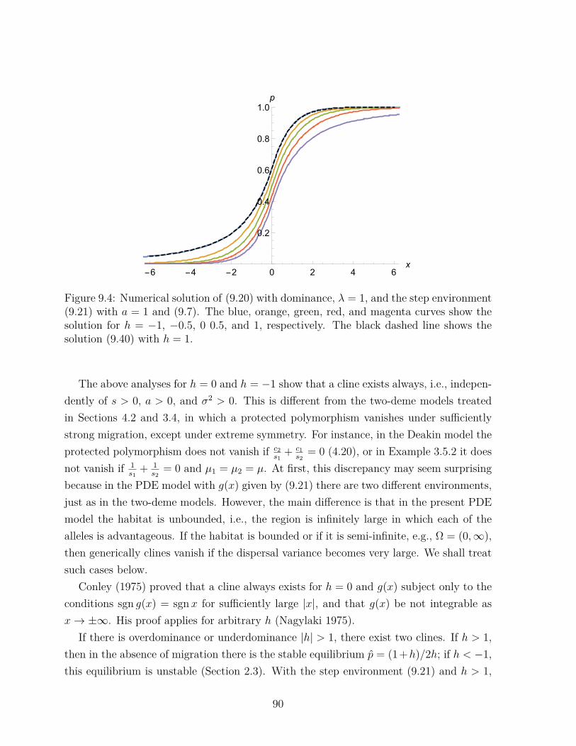
-6 -4 -2 0 2 4 6x

0.2

0.4

0.6

0.8

1.0p

Figure 9.4: Numerical solution of (9.20) with dominance, λ = 1, and the step environment(9.21) with a = 1 and (9.7). The blue, orange, green, red, and magenta curves show thesolution for h = −1, −0.5, 0 0.5, and 1, respectively. The black dashed line shows thesolution (9.40) with h = 1.

The above analyses for h = 0 and h = −1 show that a cline exists always, i.e., indepen-dently of s > 0, a > 0, and σ2 > 0. This is different from the two-deme models treatedin Sections 4.2 and 3.4, in which a protected polymorphism vanishes under sufficientlystrong migration, except under extreme symmetry. For instance, in the Deakin model theprotected polymorphism does not vanish if c2

s1+ c1

s2= 0 (4.20), or in Example 3.5.2 it does

not vanish if 1s1

+ 1s2

= 0 and µ1 = µ2 = µ. At first, this discrepancy may seem surprisingbecause in the PDE model with g(x) given by (9.21) there are two different environments,just as in the two-deme models. However, the main difference is that in the present PDEmodel the habitat is unbounded, i.e., the region is infinitely large in which each of thealleles is advantageous. If the habitat is bounded or if it is semi-infinite, e.g., Ω = (0,∞),then generically clines vanish if the dispersal variance becomes very large. We shall treatsuch cases below.

Conley (1975) proved that a cline always exists for h = 0 and g(x) subject only to theconditions sgn g(x) = sgn x for sufficiently large |x|, and that g(x) be not integrable asx→ ±∞. His proof applies for arbitrary h (Nagylaki 1975).

If there is overdominance or underdominance |h| > 1, there exist two clines. If h > 1,then in the absence of migration there is the stable equilibrium p = (1+h)/2h; if h < −1,this equilibrium is unstable (Section 2.3). With the step environment (9.21) and h > 1,

90

-10 -5 5 10x

0.2

0.4

0.6

0.8

1.0p

Figure 9.5: Numerical solution of (9.20) with h = 2, λ = 1, and the step environment(9.21) with a = 1. In the limit x → ∞, both clines converge to the pure selectionequilibrium p = (1 + h)/2h = 3/4. Which cline evolves depends on the initial data.

there is overdominance if x ≥ 0 and underdominance if x < 0. Therefore, in the presenceof migration, there will be two clines (Figure 9.5). In this case, the steepness of the clinesat x = 0 is no longer given by (9.35). An analogous formula can be derived by takinginto account the limiting behavior as x→ ±∞.

Environments other than the step environment (9.21) were investigated by Slatkin(1973) and Nagylaki (1975). The latter study is devoted to semi-infinite clines, i.e.,Ω = [0,∞). They include, for instance, the case of an environmental pocket.

9.3 Clines in a finite domain

We shall first concentrate on the simplest case, which is that of no dominance. For thiscase we shall outline the proof of the main result, Theorem 9.4. Then we shall review theavailable theory for intermediate and for complete dominance.

9.3.1 The ODE model with no dominance and two demes

To motivate the approach below for analyzing the PDE model, we recall Example 3.5.2 inwhich we investigated the ODE model for two alleles without dominance and two demes.We define

M =(−1 11 −1

)and f(p) =

(p1(1− p1)p2(1− p2)

),

91

and assume s1s2 < 0 and µ1 = µ2 = µ. After rescaling time and setting λ = 1/µ, we canrewrite the differential equation (3.35) as

p = Mp+ λ

(s1 00 s2

)f(p).

To derive the asymptotic stability of equilibria, we calculate the Jacobian and obtain

J(p) = M + λ

(s1(1− 2p1) 0

0 s2(1− 2p2)

).

Obviously, the equilibrium p = (0, 0)> is asymptotically stable if the leading eigenvalueof J(0, 0) is negative. This eigenvalue has a strictly positive eigenvector. An analogousresult holds for p = (1, 1)>.

Therefore, it is natural to study the eigenvalue problem

−J(0, 0)y = −My − λ(s1 00 s2

)y = σy, (9.42)

where λ is considered as a parameter. (In PDE theory, stationary solutions are oftencalled linearly stable if the leading eigenvalue of the linearization is positive; therefore, westudy the problem −Jy = σy.) Then p = (0, 0)> is asymptotically stable if the leadingeigenvalue σ1 > 0. Let λ1 denote a(n) (eigen)value satisfying

−My = λ1

(s1 00 s2

)y (9.43)

for a strictly positive y, i.e., y1 > 0 and y2 > 0 (provided it exists). Then we have σ1 = 0if and only if λ = λ1; one can show that σ1 > 0 if and only if 0 < λ < λ1 (we are onlyinterested in λ > 0); and σ1 < 0 if and only if λ > λ1.

From (9.43), we obtain easily that λ1 is unique and given by λ1 = 1s1

+ 1s2

(the corre-sponding eigenvector is (−s2, s1) if s1 > 0 > s2). There is a second eigenvalue, which iszero. Therefore, σ1 > 0 if and only if 1

µ= λ < λ1, which is precisely the condition for

stability of p = (0, 0)>, or non-protection of A1, i.e., κ = µs1

+ µs2> 1; cf. (4.14). Finally,

we note that λ1 = 0 if and only if s1 + s2 = 0, and λ1 > 0 if and only if s1 + s2 < 0.

9.3.2 The PDE model with no dominance

Our presentation essentially follows Lou et al. (2013). We assume that Ω is a boundedopen (connected) domain in Rn with a C2 boundary ∂Ω. We write

∆f =n∑i=1

∂2f

∂x2i

and ∇f =(∂f

∂x1, . . . ,

∂f

∂xn

)(9.44)

92

for the Laplace and the gradient (nabla) operator, respectively. Note that ∆f = ∇ · ∇f .Our goal is to study the dynamics of

∂p

∂t= ∆p+ λg(x)p(1− p) in Ω× (0,∞), (9.45a)

subject to the boundary condition

∂p

∂ν= 0 on ∂Ω× (0,∞), (9.45b)

where ∂p∂ν

= ν ·∇p denotes the derivative in direction of ν, the outward unit normal vectoron ∂Ω, and

0 ≤ p(x, 0) ≤ 1, p(x, 0) . 0, p(x, 0) . 1 in Ω. (9.45c)

If n = 1 then Ω = (b1, b2), where −∞ < b1 < b2 < ∞. In this much simpler one-dimensional case, the equilibrium solution of (9.45) can be determined from the ordinarydifferential equation

p′′ + λg(x)p(1− p) = 0, (9.46)

and the boundary condition (9.45b) simplifies to

p′(b1, t) = p′(b2, t) = 0 for t ∈ (0,∞). (9.45b’)

The following eigenvalue problem will play a crucial role in our investigation of thedynamics (9.45):

−∆ϕ = λg(x)ϕ in Ω, (9.47a)∂ϕ

∂ν= 0 on ∂Ω× (0,∞) and ϕ > 0 in Ω. (9.47b)

[This problem arises as follows. Linearization of the parabolic operator defined by L(p) =∂p/∂t − ∆p − λg(x)p(1 − p) and evaluation at a stationary solution p∗ yields DL|p∗ =−∆ − λg(x)(1 − 2p∗). Therefore, linear stability of the stationary solution p∗ can bedetermined by studying the eigenvalue problem −∆ϕ− λg(x)(1− 2p∗)ϕ = σϕ. If p∗ is atrivial solution (p∗ ≡ 0 or p∗ ≡ 1), a problem of the form (9.47) emerges from the criticalcase in which the principal eigenvalue of DL|p∗ is σ = 0.]

We say that λ is a principal eigenvalue of (9.47) if (9.47) has a solution. Clearly, zero isalways a principal eigenvalue of (9.47) with positive constants as eigenfunctions. However,only positive principal eigenvalues of (9.47) are relevant in analyzing the dynamics of(9.45). In the one-dimensional (ODE) case, (9.47) is a special case of the Sturm-Liouvilleeigenvalue problem. Our first result is the following:

93

Proposition 9.1. Suppose that g is not identically zero. Then (9.47) has a positiveeigenvalue, λ1(g), if and only if g changes sign in Ω and∫

Ωg(x)dx < 0. (9.48)

For the one-dimensional case, this problem was solved by Picone (1910) and Bocher(1914) using Sturm’s theory. The n-dimensional case was settled by Brown and Lin(1980), the general elliptic case by Senn and Hess (1982). We will proof this result inSection 9.3.3.

Remark 9.2. We note the analogy to the two-deme model outlined in Section 9.3.1, in

which M plays the role of ∆ and(s1 00 s2

)that of g.

Remark 9.3. It is well known that if the principle eigenvalue λ1(g) of (9.47) exists, it issimple and its corresponding eigenfunction can be chosen positive in Ω. Moreover, if λ isa positive eigenvalue of (9.47), then λ ≥ λ1(g). Hence, we call λ1(g) the smallest positiveeigenvalue of (9.47). No other eigenvalue than λ1(g) has an eigenfunction that does notchange sign. We will prove these statements in Section 9.3.3.

We call an equilibrium globally asymptotically stable if it is asymptotically stable andevery solution p(x, t) of (9.45a) satisfying the initial condition (9.45c) converges to ituniformly, i.e., in L∞(Ω).

The following is the main result of this section.

Theorem 9.4. (i) Suppose that∫

Ω g(x)dx < 0 and g changes sign in Ω. If λ ≤ λ1(g), theequilibrium p ≡ 0 of (9.45) is globally asymptotically stable. If λ > λ1(g), then (9.45) hasa unique equilibrium p satisfying 0 < p < 1 in Ω, which is globally asymptotically stable.

(ii) Suppose that∫Ω g(x)dx = 0 and g changes sign in Ω. Then for every λ > 0, (9.45)

has a unique nontrivial equilibrium, which is globally asymptotically stable.(iii) Suppose that

∫Ω g(x)dx > 0 and g changes sign in Ω. There exists a λ∗ > 0 such

that if 0 < λ ≤ λ∗, then p ≡ 1 is globally asymptotically stable. If λ > λ∗, then (9.45)has a unique equilibrium p∗ satisfying 0 < p∗ < 1 in Ω, which is globally asymptoticallystable.

A non-trivial equilibrium of (9.45) is not constant because this would imply g ≡ 0. Itrepresents a cline. The proof of Theorem 9.4 consists of four main steps and is deferredto Section 9.3.4. First, the (linear) stability properties of the trivial equilibria (p ≡ 0and p ≡ 1) will be established with the help of Proposition 9.1. Then the method of

94

super- and subsolutions will be employed to establish existence of a nontrivial equlibriumif both trivial equilibria are unstable. In the third step, linear stability of any nontrivialequilibrium will be proved, and degree theory will establish uniqueness. Finally, globalconvergence is proved using a Lyapunov function.

Remark 9.5. Fleming (1975) derived the conditions for the stability of the trivial solu-tions p ≡ 0 and p ≡ 1 and proved existence of a stable nontrivial solution if both trivialsolutions are unstable. Henry (1981) proved the above result for the Laplace operator onan open bounded domain in Rn. Lou and Nagylaki (2002, Theorem 2.1) generalized thisto arbitrary elliptic operators on an open bounded domain in Rn, in particular to multi-variate versions of the differential operator occurring in (8.12). Thus, their result appliesto much more general migration patterns, which need not to be isotropic or homogeneous.Also varying population density is covered by their model.

Remark 9.6. 1. We point out the analogy to the results about protection of alleles andexistence of a stable equilibrium in Sections 4.2 and 3.4. The condition

∫Ω g(x)dx < 0

generalizes the condition s1+s2 < 0. Therefore, A1 is not protected (p = 0 asymptoticallystable) if κ = µ/s1 + µ/s2 > 1 and protected if κ < 1. In the latter case, we indeed havea protected polymorphism because κ > 0 if s1 + s2 < 0. As already noted at the end ofSection 9.3.1, we have κ = µλ1 = λ1/λ. Therefore, the condition λ > λ1(g) in Theorem9.4 (i) corresponds to κ < 1.

2. If s1 + s2 = 0, then κ = 0 for every µ > 0 and a stable interior equilibrium existsalways, just as if

∫Ω g(x) dx = 0.

3. We recall from Section 9.2.1 that for the step environment in Ω = (−∞,∞), a clineexists for every λ > 0 even if the selection is asymmetric.

The following result shows that (in the sense specified) the cline gets steeper as selectiongets stronger or dispersal weaker.

Proposition 9.7. For λ > λ1(g), i.e., when the cline p exists, ‖∇p‖L2(Ω) is a strictlymonotone increasing function of λ.

For the proof, see Lou et al. (2013).

9.3.3 ∗Proof of Proposition 9.1

We first establish necessity. If (9.47) has a positive eigenvalue with eigenfunction ϕ > 0in Ω, then by the strong maximum principle for elliptic equations (Appendix C), we have

95

ϕ > 0 in Ω. (In the one-dimensional case, this follows from the elementary Theorem C.1.)Therefore, dividing (9.47a) by ϕ and integrating over Ω, we obtain by using Green’s firstidentity8 (partial integration in the 1-d case) and observing the boundary condition on ϕ(9.47b) ∫

Ωg(x) dx = 1

λ

∫Ω−ϕ−1∆ϕdx

= 1λ

(∮∂Ω−ϕ−1∂ϕ

∂νdS +

∫Ω∇(ϕ−1) · ∇ϕdx

)

= −1λ

∫Ω

|∇ϕ|2

ϕ2 dx < 0, (9.49)

where the last inequality is strict because ϕ is not constant. (If ϕ were constant, then g ≡ 0would follow from (9.47a), a contradiction to our assumption.) Furthermore, integrating(9.47a) in Ω, we find by a similar calculation

∫Ω g(x)ϕ(x) dx = 0, which together with

positivity of ϕ implies that g must change sign.The proof of sufficiency is deeper. In a series of lemmas, we will show that

λ1(g) = infψ∈S

K(g, ψ) (9.50)

is the desired eigenvalue. Here,

K(g, ψ) = −∫

Ω ψ∆ψ dx∫Ω gψ

2 dx=∫

Ω |∇ψ|2 dx∫

Ω gψ2 dx

(9.51)

is a ‘Rayleigh quotient’ and

S = ψ ∈ H1(Ω) :∫

Ωgψ2 > 0 and ∂ψ/∂ν = 0 on ∂Ω, (9.52)

where H1(Ω) is the Sobolov space in L2(Ω) with weak derivatives of first order in L2(Ω)(D.2) (Appendix D). Essentially, the proof follows Brown and Lin (1980). Indeed, we willalso prove most of the statements of Remark 9.3.

We define

Qλ(ψ) = 〈−∆ψ, ψ〉 − λ∫

Ωgψ2 dx =

∫Ω|∇ψ|2 dx− λ

∫Ωgψ2 dx, (9.53)

where 〈u, v〉 =∫Ω uv dx. Then Qλ(ψ) ≥ 0 if and only if λ ≤ K(g, ψ), and

Qλ(ψλ) = 0 (9.54)

if λ is an eigenvalue of (9.47) with eigenfunction ψλ.8∫

Ω(ψ∆ϕ+∇ψ · ∇ϕ) dx =∮∂Ω ψ

∂ϕ∂ν dS

96

Remark 9.8. The variational characterization (9.50) of λ1(g) is related to Courant’sMinimum-Maximum Principle (and to the min-max principle for Hermitian matrices).For Hermitian matrices, the Rayleigh quotient is simply (Ax, x)/(x, x) (cf. Appendix E).

Lemma 9.9. If there is a nonnegative eigenfunction of (9.47), then Qλ(ψ) ≥ 0 for everyψ ∈ S. Therefore, any eigenvalue λ of (9.47) with a nonnegative eigenfunction satisfiesλ ≤ λ1(g).

Proof. OnD(L1) = u ∈ H2(Ω) : ∂u/∂ν = 0 on ∂Ω, (9.55)

we define the operators L1u = −∆u and

(Tu)(x) = −∆u(x)− λg(x)u(x) for x ∈ Ω, (9.56)

Then T is self-adjoint and its spectrum consists of the eigenvalues µ1 < µ2 ≤ . . .. Theeigenvalue µ1 is simple and the corresponding eigenfunction ψ1 can be chosen such thatψ1 > 0 in Ω (Appendix E). Now suppose that ϕ is a nonnegative eigenfunction of (9.47).Therefore, µ1 = 0 must be an eigenvalue of T . Because only the smallest eigenvaluehas a nonnegative eigenfunction, and its eigenspace is one-dimensional, ϕ must pertain toµ1 = 0. From the spectral decomposition (Remark E.7), we obtain 〈Tu, u〉 ≥ µ1〈u, u〉 = 0,i.e., Qλ(u) ≥ 0, for every u ∈ D(L1).

Lemma 9.10. Let∫

Ω g dx < 0. Then there exist β > 0 and γ > 0 such that∫Ω|∇ψ|2 dx ≥ β

∫Ωψ2 dx (9.57)

for all ψ ∈ D(L1) satisfying∫

Ω gψ2 dx > −γ

∫Ω ψ

2 dx.

Proof. The proof is by contradiction. Suppose that ψn ⊂ D(L1) such that∫

Ω ψ2n dx = 1,∫

Ω |∇ψn|2 dx ≤ 1/n, and

∫Ω gψ

2n dx ≥ −1/n for every n. Then ψn is bounded in

H1(Ω) and therefore has a subsequence, ψk, that converges to some ψ ∈ L2(Ω). Since∫Ω |∇ψk|

2 dx ≤ 1/k for all k, ψk is a Cauchy sequence in H1(Ω), thus converges toψ ∈ H1(Ω), which satisfies∫

Ωψ2 dx = 1,

∫Ω|∇ψ|2 dx = 0, and

∫Ωgψ2 dx ≥ 0. (9.58)

The first two properties imply that ψ ≡ c , 0, hence∫

Ω gψ2 dx = c

∫Ω g dx < 0, a

contradiction.

97

The following result is quite intuitive because ψ = const < S if∫

Ω g dx < 0, however,its proof relies on Lemma 9.10.

Lemma 9.11. If∫

Ω g dx < 0, then λ1(g) > 0.

Proof. For ψ ∈ S, we have∫

Ω gψ2 dx > 0 and

K(g, ψ) =∫

Ω |∇ψ|2 dx∫

Ω gψ2 dx

≥∫

Ω |∇ψ|2 dx

maxx∈Ω |g(x)|∫

Ω ψ2 dx

≥ β/maxx∈Ω|g(x)| ,

where the last inequality is from Lemma 9.10. Thus, λ1(g) ≥ β/maxx∈Ω |g(x)| > 0.

Lemma 9.12. Let∫Ω g dx < 0. If λ > λ1(g), then λ is not an eigenvalue with a nonneg-

ative eigenfunction. If 0 < λ < λ1(g), then λ is not an eigenvalue.

Proof. The first statement is already contained in Lemma 9.9. To prove the secondstatement, by (9.54) it is sufficient to show that (for given λ) there exists a > 0 such thatQλ(ψ) ≥ a‖ψ‖2 for every ψ ∈ D(L1).

Let λ = (1− τ)λ1(g), where 0 < τ < 1 and ψ ∈ D(L1). Then

Qλ(ψ) =∫

Ω|∇ψ|2 dx− λ

∫Ωgψ2 dx

= λ

λ1Qλ1(ψ) +

(1− λ

λ1

)∫Ω|∇ψ|2 dx ≥ τ

∫Ω|∇ψ|2 dx.

Let β and γ be the constants in Lemma 9.10. If∫

Ω gψ2 dx > −γ

∫Ω ψ

2 dx, we obtain from(9.57)

Qλ(ψ) ≥ τ∫

Ω|∇ψ|2 dx ≥ τβ‖ψ‖2. (9.59)

If∫

Ω gψ2 dx ≤ −γ

∫Ω ψ

2 dx, we have

Qλ(ψ) =∫

Ω|∇ψ|2 dx− λ

∫Ωgψ2 dx ≥ λγ‖ψ‖2. (9.60)

Lemma 9.13. If∫

Ω g dx < 0, then λ1(g) is a simple eigenvalue with an eigenfunctionthat can be chosen positive on Ω.

Proof. We consider the linear eigenvalue problem

−∆ϕ− λ1(g)g(x)ϕ = σϕ in Ω, (9.61a)∂ϕ

∂ν= 0 on ∂Ω (9.61b)

98

and define the operator T1 : D(L1)→ L2(Ω) by

(T1u)(x) = −∆u(x)− λ1(g)g(x)u(x). (9.62)

Then λ1(g) is an eigenvalue of (9.47) with corresponding eigenfunction ϕ if and only if0 is an eigenvalue of T1, hence of (9.61), with corresponding eigenfunction ϕ. The leasteigenvalue σ1 of T1 is given by

σ1 = infQλ1(ψ) : ψ ∈ D(L1) (9.63)

(Theorem E.9). Since Qλ1(ψ) ≥ 0 for all ψ ∈ D(L1), we have σ1 ≥ 0. From the definitionof λ1(g) it follows that there is a sequence ψn ⊂ D(L1) such that

∫Ω gψ

2n dx = 1

and limn→∞∫Ω |∇ψn|

2 dx = λ1(g). Therefore, limn→∞Qλ1(ψn) = 0, whence σ1 = 0.Therefore, σ1 = 0 is the smallest eigenvalue of (9.61), hence simple and the correspondingeigenfunction can be chosen positive on Ω. By the strong maximum principle, it is positiveon Ω.

Obviously, Lemma 9.13 completes the proof of sufficiency in Proposition 9.1. Theother lemmas show that λ1(g) > 0 and that λ1(g) is the only positive eigenvalue with thedesired properties.

9.3.4 ∗Proof of Theorem 9.4 (i)

Throughout, we assume∫Ω g(x) dx < 0 and g changes sign in Ω.

(a) First, we investigate the local stability of the equilibria p ≡ 1 and p ≡ 0.

Lemma 9.14. The equilibrium p ≡ 1 is unstable for every λ > 0.

Proof. The linearization of the right-hand side of (9.45a) evaluated at p ≡ 1 is ∆−λg(x).Therefore, p ≡ 1 is asymptotically stable (in the Lyapunov sense) if the smallest eigenvalueσ1 of

−∆ψ + λg(x)ψ = σψ in Ω, (9.64a)∂ψ

∂ν= 0 on ∂Ω, ψ > 0 in ∂Ω (9.64b)

is positive. It is unstable if σ1 < 0. This smallest eigenvalue exists, is simple, and has aneigenfunction ψ1 > 0 on Ω (Appendix E). We infer from (9.64)

−∆ψ1

ψ1+ λg(x) = σ1 (9.65)

99

and, by integration,

−∫

Ω

|∇ψ1|2

ψ21

dx+ λ∫

Ωg dx = |Ω|σ1. (9.66)

Our assumptions imply that σ1 < 0 if λ > 0.

Now we turn to the more interesting and important stability of the equilibrium p ≡ 0.We recall that λ1(g) is the principal, i.e., smallest positive, eigenvalue of (9.47). It existsby Proposition 9.1.

Lemma 9.15. The equilibrium p ≡ 0 is asymptotically stable if 0 < λ < λ1(g) andunstable if λ > λ1(g).

Proof. The linearization of the right-hand side of (9.45a) evaluated at p ≡ 0 is ∆+λg(x).Therefore, p ≡ 0 is asymptotically stable if the smallest eigenvalue σ1 of

−∆ϕ− λg(x)ϕ = σϕ in Ω, (9.67a)∂ϕ

∂ν= 0 on ∂Ω (9.67b)

is positive. This smallest eigenvalue exists, is simple, and has an eigenfunction ϕ1 > 0 onΩ (Appendix E).

We claim that

σ1

> 0 if 0 < λ < λ1(g),= 0 if λ = λ1(g),< 0 if λ > λ1(g).

(9.68)

Obviously, this claim establishes the lemma (see the left panel in Fig. 9.6).Let us consider σ1 as a function of λ. Because σ1(0) = σ1(λ1(g)) = 0, (9.68) is an

immediate consequence of Lemma 9.16 below.

Lemma 9.16. If g is a nonconstant function, then σ1(λ) is strictly concave downward.

Proof. By the variational characterization of σ1(λ) (Appendix E, Theorem E.9), we obtainfor any pair λ , λ

σ1(

12(λ+ λ)

)= infψ∈H1,

∫Ω ψ

2=1

∫Ω

[|∇ψ(x)|2 − 1

2(λ+ λ)g(x)ψ(x)2]dx

= infψ∈H1,

∫Ω ψ

2=1

[12

∫Ω

(|∇ψ|2 − λgψ2) dx+ 12

∫Ω

(|∇ψ|2 − λgψ2) dx]

100

>12 infψ∈H1,

∫Ω ψ

2=1

∫Ω

(|∇ψ|2 − λgψ2) dx+ 12 infψ∈H1,

∫Ω ψ

2=1

∫Ω

(|∇ψ|2 − λgψ2) dx

= 12[σ1(λ) + σ1(λ)],

where the inequality is strict because the eigenfunctions of σ1(λ) and σ1(λ) are linearlyindependent (since g is not constant).

(b) Now we establish existence of a nontrivial equilibrium (the cline). We apply thesupersolution-subsolution method to show that if λ > λ1(g), then (9.45) has at least onenontrivial equilibrium p, i.e., p satisfies 0 < p < 1 in Ω.

To establish a subsolution for given λ > λ1(g), let ϕ1 denote the eigenfunction of thesmallest eigenvalue σ1 of (9.67) that is uniquely determined by maxΩ ϕ1 = 1. Set p = εϕ1,where ε > 0 is to be determined. Hence,

∆p+ λgp(1− p) = ∆(εϕ1) + λgεϕ1 − λgε2ϕ21

= −σ1εϕ1 − λgε2ϕ21

= (−σ1 − ελgϕ1)εϕ1 > 0, (9.69)

where the inequality holds if 0 < ε < −σ1(λ)/(λ‖g‖∞) because σ1(λ) < 0 if λ > λ1(g).To establish a supersolution, let ψ1 denote the eigenfunction of the smallest eigenvalue

σ1 of (9.64) such that maxΩ ψ1 = 1. Set p = 1− εψ1. As above, one shows easily that

∆p+ λgp(1− p) = εψ1(σ1 − ελgψ1) < 0, (9.70)

where the inequality holds if 0 < ε < −σ1/(λ‖g‖∞) because σ1 < 0 for every λ > 0.By the supersolution and subsolution method (e.g., Cantrell and Cosner 2003), for any

λ > λ1(g), the problem (9.45) has at least one equilibrium p satisfying p < p < p in Ω.(c) Next, we show uniqueness of the nontrivial equilibrium and asymptotic stability.

A main ingredient is

Lemma 9.17. Any equilibrium p∗ of (9.45) satisfying 0 < p∗ < 1 is asymptotically stable;in particular, it is nondegenerate and isolated.

Proof. The linearized stability of p∗ is determined by the smallest eigenvalue (denoted asσ1) of

−∆ψ − λg(1− 2p∗)ψ = σψ in Ω, ∂ψ

∂ν= 0 on ∂Ω. (9.71)

Let ψ1 > 0 denote an eigenfunction of σ1, i.e.,

∆ψ1 + λg(1− 2p∗)ψ1 = −σ1ψ1. (9.72)

101

Figure 9.6: The eigenvalue σ1(λ).

Multiplying (9.72) by f(p∗) = p∗(1 − p∗) and integrating (using Green’s identity and∂ψ1∂ν

= 0), we find

− σ1

∫Ωp∗(1− p∗)ψ1 dx =

∫Ωp∗(1− p∗)∆ψ1 dx+ λ

∫Ωp∗(1− p∗)g(1− 2p∗)ψ1 dx

= −∫

Ω∇(p∗(1− p∗)) · ∇ψ1 dx+ λ

∫Ωgp∗(1− p∗)(1− 2p∗)ψ1 dx

= −∫

Ω(1− 2p∗)∇(p∗) · ∇ψ1 dx+ λ

∫Ωgp∗(1− p∗)(1− 2p∗)ψ1 dx. (9.73)

Recalling (9.45a), i.e., ∆p∗+λg(x)p∗(1−p∗) = 0, multiplying the equation by (1−2p∗)ψ1

and integrating, we obtain after a similar calculation

2∫

Ωψ1 |∇p∗|2 dx−

∫Ω

(1−2p∗)∇(p∗) ·∇ψ1 dx+λ∫

Ωgp∗(1−p∗)(1−2p∗)ψ1 dx = 0. (9.74)

From (9.73) and (9.74) we infer

σ1

∫Ωp∗(1− p∗)ψ1 dx = 2

∫Ωψ1 |∇p∗|2 dx > 0, (9.75)

where the inequality is strict because ψ1 > 0 in Ω and p∗ is not constant. Hence, σ1 > 0and the lemma is proved.

This lemma settles not only asymptotic stability of any equilibrium p∗ satisfying 0 <p∗ < 1, but also uniqueness as we show now. Because both trivial equilibria p ≡ 0 andp ≡ 1 are isolated, the construction of the supersolution p and subsolution p implies forsufficiently small ε that all nontrivial equilibria must lie between p and p. It is well knownthat the total (Leray-Schauder) degree (e.g., O’Regan et al., 2006) of nontrivial equilibriabetween a supersolution and a subsolution is equal to one. Hence, the total degree of

102

Figure 9.7: Bifurcation diagram for the model (9.78) with no dominance.

all nontrivial equilibria is equal to one. By Lemma 9.17, each nontrivial equilibrium islinearly stable, so it must be isolated and have Leray-Schauder degree one. Therefore,(9.45) has at most one nontrivial equilibrium.

(d) For the proof of global convergence, we refer to Henry (1981) or Lou and Nagylaki(2002). For the Laplace operator global convergence follows from the fact that (9.45) is agradient system with ‘potential’

V (u) =∫

Ω

[∇u · ∇u− λg(u2 − 2

3u3)]dx. (9.76)

Indeed,

dV

dt(u) =

∫Ω

[2∇u · ∇ut − λg(2uut − 2u2ut)

]dx

= 2∫

Ω[−∆u− λgu(1− u)]ut dx

= 2∫

Ω−u2

t dx ≤ 0,

where the second equality uses Green’s identity and the last follows from (9.45a). Fromthe theory of gradient systems together with compactness arguments, one can concludethat the ω-limit set of any solution contains only equilibria. Because there exists only oneasymptotically stable equilibrium, global convergence follows.

The bifurcation diagram in Figure 9.7 illustrates the equilibrium and stability proper-ties formulated in statement (i) of Theorem 9.4.

9.3.5 ∗Proof of Theorem 9.4 (ii), (iii)

The proofs of statements (ii) and (iii) are very similar to the proof of (i). Statements (i)and (iii) are symmetric upon interchanging the roles of the equilibria p ≡ 0 and p ≡ 1.The key observation in the proof of (ii) is that if

∫Ω g dx = 0, then σ(λ) ≤ 0 for every λ

103

and equality holds only if λ = 0; see Fig. 9.6. The shapes of σ1(λ) displayed in Fig. 9.6follow from Lemma 9.16 and the following calculation.

Let ϕ′ = ∂ϕ∂λ

(x, λ). Then differentiation of (9.67) with respect to λ yields

−∆ϕ′ − λg(x)ϕ′ − g(x)ϕ = σ′1(λ)ϕ+ σ1(λ)ϕ′ in Ω,∂ϕ′

∂ν= 0 on ∂Ω.

Evaluation at λ = 0 produces

−∆ϕ′∣∣∣∣λ=0−g(x) = σ′1(0) in Ω,

∂ϕ′

∂ν= 0 on ∂Ω

because σ1(0) = 0 and the corresponding eigenfunction can be chosen ϕ ≡ 1. Finally,integration yields

σ′1(0) = − 1|Ω|

∫Ωg(x) dx. (9.77)

9.4 ∗Clines in a finite domain with dominance: Results and openproblems

In this section, we review the most important results about the existence of clines in thepresence of dominance. We will also mention some open problems. Our exposition islargely based on the review of Lou et al. (2013). We focus on the following PDE:

∂p

∂t= ∆p+ λg(x)f(p) in Ω× (0,∞), (9.78a)

∂p

∂ν= 0 on ∂Ω× (0,∞), (9.78b)

0 ≤ p(x, 0) ≤ 1, p(x, 0) . 0, p(x, 0) . 1 in Ω, (9.78c)

where f ∈ C1([0, 1]), f(0) = f(1) = 0 and f > 0 in (0, 1). The most important exampleis

f(p) = p(1− p)(1 + h− 2hp), (9.79)

where −1 ≤ h ≤ 1, i.e., dominance is intermediate; cf. eqs. (9.4) – (9.8). Throughout wesuppose that g changes sign.

First, we contrast the case of no dominance with that of complete dominance.

104

9.4.1 Complete dominance

We assume complete dominance of A2, or recessivity of A1, i.e.,

f(p) = 2p2(1− p); (9.80)

cf. (9.6). This case turns out to be quite different from that of no dominance. In fact,this is already obvious from the model with two demes.

One reason why the model with complete dominance is more complicated than withno dominance is that the equilibrium p ≡ 0 is degenerate. Indeed, the linearization of theright-hand side of (9.78a) is ∆ + 2λgp(2 − 3p) which simplifies to ∆ at p ≡ 0. Hence, 0is an eigenvalue. Nevertheless, the following result can be proved:

Theorem 9.18 (Lou et al. 2010).(i) If

∫Ω g dx ≥ 0, then p ≡ 0 is unstable for every λ > 0.

(ii) If∫

Ω g dx < 0, then p ≡ 0 is stable for every λ > 0.

Obviously, statement (ii) differs markedly from Lemma 9.15 for no dominance.The equilibrium p ≡ 1 is not degenerate because f ′(1) = −2. Therefore, its stability

properties follow from Sections 9.3.4 and 9.3.5. It is unstable for every λ > 0 if∫

Ω g dx ≤ 0.If∫

Ω g dx > 0, there exists λ∗ > 0 such that p ≡ 1 is stable if 0 < λ < λ∗ and unstable ifλ > λ∗ (cf. Theorem 9.4).

In addition, the following results have been proved:

Theorem 9.19 (Lou et al. 2010, Nakashima et al. 2010).(i) If

∫Ω g dx , 0, then for sufficiently small λ > 0, (9.78) has no nontrivial equilibrium.

(ii) If∫

Ω g dx < 0, then for sufficiently large λ, (9.78) has at least two nontrivialequilibria, one stable and one unstable.

(iii) If∫

Ω g dx > 0, then for sufficiently large λ, (9.78) has a stable nontrivial equilib-rium.

Theorem 9.20 (Nakashima et al. 2010). Suppose that∫

Ω g dx = 0.(i) For every λ > 0, (9.78) has at least one stable nontrivial equilibrium p∗.(ii) As λ → 0+, any sequence of nontrivial equilibria of (9.78) has a subsequence

converging to the constant function 2/3 in C2(Ω).(iii) As λ→∞, p∗ → 1 uniformly on any compact subset of Ω+\∂Ω+ ∩ Ω, and p∗ → 0

uniformly on any compact subset of Ω− \ ∂Ω− ∩ Ω, where Ω+ = x ∈ Ω : g(x) > 0 andΩ− = x ∈ Ω : g(x) < 0.

105

Figure 9.8: Bifurcation diagrams for the model (9.78) with complete dominance.

Recently, Nakashima (2016) established uniqueness of the solution in statement (iii) ofTheorem 9.19 and of that in statement (i) of Theorem 9.20 for one spatial dimension andif g changes sign once. Generalizations to functions g(x) which change sign more thanonce were derived in Nakashima (2018).

The main results are illustrated in Figure 9.8. They should be compared with thebifurcation diagram for the case of no dominance (Figure 9.7).

Analogs of the above results, in fact considerably stronger results, were derived byNagylaki (2009) for the continuous-time two-deme model. He proved that the number ofequilibria is precisely one or two in the above theorems instead of at least one or two. Ifthere is only a single stable equilibrium, it is globally asymptotically stable. Therefore,Figure 9.8 illustrates his results precisely. Whether this is also true for the PDE model(i.e., if the number of equilibria is as in this figure) is an open problem. As brieflydiscussed in Lou et al. (2013), the structure of the nontrivial equilibria in the PDE model(9.78) with complete dominance may be more complicated than in the ODE case withtwo demes.

106

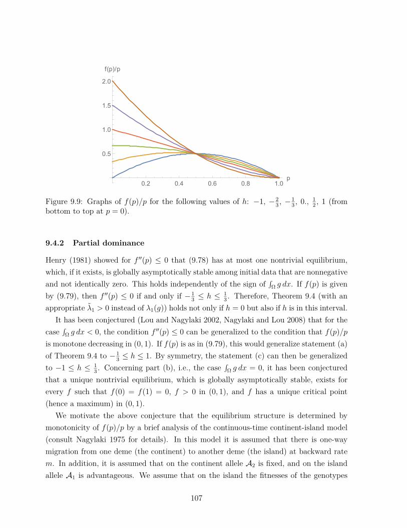
0.2 0.4 0.6 0.8 1.0p

0.5

1.0

1.5

2.0

f(p)/p

Figure 9.9: Graphs of f(p)/p for the following values of h: −1, −23 , −1

3 , 0., 12 , 1 (from

bottom to top at p = 0).

9.4.2 Partial dominance

Henry (1981) showed for f ′′(p) ≤ 0 that (9.78) has at most one nontrivial equilibrium,which, if it exists, is globally asymptotically stable among initial data that are nonnegativeand not identically zero. This holds independently of the sign of

∫Ω g dx. If f(p) is given

by (9.79), then f ′′(p) ≤ 0 if and only if −13 ≤ h ≤ 1

3 . Therefore, Theorem 9.4 (with anappropriate λ1 > 0 instead of λ1(g)) holds not only if h = 0 but also if h is in this interval.

It has been conjectured (Lou and Nagylaki 2002, Nagylaki and Lou 2008) that for thecase

∫Ω g dx < 0, the condition f ′′(p) ≤ 0 can be generalized to the condition that f(p)/p

is monotone decreasing in (0, 1). If f(p) is as in (9.79), this would generalize statement (a)of Theorem 9.4 to −1

3 ≤ h ≤ 1. By symmetry, the statement (c) can then be generalizedto −1 ≤ h ≤ 1

3 . Concerning part (b), i.e., the case∫

Ω g dx = 0, it has been conjecturedthat a unique nontrivial equilibrium, which is globally asymptotically stable, exists forevery f such that f(0) = f(1) = 0, f > 0 in (0, 1), and f has a unique critical point(hence a maximum) in (0, 1).

We motivate the above conjecture that the equilibrium structure is determined bymonotonicity of f(p)/p by a brief analysis of the continuous-time continent-island model(consult Nagylaki 1975 for details). In this model it is assumed that there is one-waymigration from one deme (the continent) to another deme (the island) at backward ratem. In addition, it is assumed that on the continent allele A2 is fixed, and on the islandallele A1 is advantageous. We assume that on the island the fitnesses of the genotypes

107

A1A1, A1A2, and A2A2 are s, hs, and −s, respectively; cf. Sections 4 and 5. If thefrequency of A1 on the island is denoted by p, its evolution is described by the ODE

p = −mp+ sf(p), (9.81)

where f(p) is given by (9.79). The equilibria are given by the solutions of

m

s= f(p)

p= (1− p)(1 + h− 2hp). (9.82)

Obviously, there exists no solution in (0, 1) if m/s > µ1 = max0≤p≤1f(p)p

. In this case,p = 0 is globally asymptotically stable. If m/s < µ1, there exist one or two solutions. Iff(p)/p is strictly monotone decreasing on [0, 1], which is the case if and only if−1

3 ≤ h ≤ 1,then there exists a unique solution for every m/s < µ1. If f(p)/p is not strictly monotonedecreasing, there exist two equilibria if µ2 < m/s < µ1, where µ2 = limp→0

f(p)p

= 1 + h,and one equilibrium if 0 ≤ m/s ≤ µ2 (cf. Figure 9.9). If two nontrivial equilibria exist,the one with the lower equilibrium frequency of p is unstable, the other is asymptoticallystable, as is p = 0. If only one nontrivial equilibrium exists, it is globally asymptoticallystable.

This model has been generalized by assuming discrete time (Nagylaki 1992) and byadmitting evolution on the continent (Nagylaki 2009). The analysis of these discrete-timemodels is much more complicated. Also the results differ slightly because the criticalvalue for h below which a pair of nontrivial equilibria may exist depends on m and isbetween −1 and −1

3 .Recently, Sovrano (2018) disproved the conjecture by Lou and Nagylaki by providing

examples of functions f(p) such that f(p)/p is strictly monotone decreasing (but f(p)not concave) that give rise to at least three non-trivial equilibrium solutions of (9.78). InFeltrin and Sovrano (2018), results about the multiplicity of such solutions are derivedby phase-portrait methods and functions f(p) are constructed that yield high multiplicity(up to 8).

9.5 ∗Further directions

Several generalizations and variants of the cline models treated above have been investi-gated. Here, we give a very brief guide to the most relevant literature.

For a bounded domain Ω ⊂ Rn, a considerably body of theory has been developedfor models with arbitrary migration, i.e., elliptic operators, and for multiple alleles (Louand Nagylaki 2002, 2004, 2006; Nagylaki and Lou 2008). Most of this work is devoted

108

to either necessary or sufficient conditions for the loss of one or several alleles, or for themaintenance of a polymorphism. However, already for three alleles and in the absence ofdominance the dynamics may become rather complex (Lou and Nagylaki 2006).

Interesting and important problems occur if migration varies within the spatial domain,for instance because of a barrier, if migration is asymmetric, or if population densityvaries. Such models have been studied by Slatkin (1973), Nagylaki (1976, 1978, 1996),ten Eikelder (1979), Fife and Peletier (1981), Pauwelussen and Peletier (1981), Pialek andBarton (1997).

In the classical treatments of clines, the domain is assumed to be (−∞,∞). It is inthis case that explicit solutions can be derived (Section 9.2). The mathematical theory,however, has been further developed under the assumption of a bounded domain (Section9.3). Despite additional technical complications, also for an unbounded domain importantresults have been proved (e.g., ten Eikelder 1979, Fife and Peletier 1981, Pauwelussen andPeletier 1981). An important special case is that of an environmental pocket, in whichone allele is favored in a bounded interval whereas the alternative allele is favored in theunbounded complement. This situation can be efficiently modeled on the domain [0,∞)(or its higher dimensional generalizations) and leads to semi-infinite clines (Nagylaki 1975,Tertikas 1988, Brown and Tertikas 1991). For environments such as a step environment,these models admit solutions that are almost as explicit as for the step environment on(−∞,∞). They share interesting properties with models of continent-island type.

In a recent series of papers, Nagylaki and collaborators extended the diffusion model,which approximates short-distance migration, to models that include short- and long-distance migration. The latter is approximated by assuming that a fraction of the pop-ulation reproduces panmicticly. It gives rise to an integral term so that the resultingmodel becomes an integro-PDE model. Numerous aspects of the classical theory havebeen extended to this setting, and qualitatively new results and properties have beenfound. However, many challenging open problems remain (Nagylaki 2012a,b; Lou et al.2013; Nagylaki and Zeng 2014; Nagylaki et al. 2014; Su and Nagylaki 2015; Nagylaki etal. 2019; and references therein).

Acknowledgments

Many thanks to Prof. Thomas Nagylaki, Dr. Linlin Su, and Sarah Henze for commentsand for pointing out errors. Special thanks go to Dr. Linlin Su for providing Appendix E.

109

A Appendix: Perron–Frobenius theory

In this appendix we summarize some important results from the spectral theory of non-negative matrices. These were discovered by Perron and Frobenius around 1910 and areuseful tools in proving existence, uniqueness, positivity, and stability of equilibrium so-lutions in many discrete-time or continuous-time models. For a more complete accountof the spectral theory of nonnegative matrices, including proofs, the reader is referred toGantmacher (1959), Schaefer (1974, Chapter I), or Seneta (1981). The latter referencecontains, in particular, a detailed treatment of countably infinite matrices.

A k × k matrix A = (aij) is called nonnegative, A ≥ 0, if aij ≥ 0 for every i, j. It iscalled positive, A > 0, if aij > 0 for every i, j. Similarly, a vector x = (x1, . . . , xk)> is saidto be nonnegative (positive) if xi ≥ 0 (xi > 0) for every i.

The spectral radius r = r(A) of an arbitrary matrix A is the radius of the smallest circlein the complex plane that contains all eigenvalues of A, i.e., |λ| ≤ r for all eigenvaluesλ of A. It can be shown that r = limn‖An‖1/n, where ‖A‖ is an arbitrary norm of thematrix A, e.g., ‖A‖ = maxi

∑kj=1 |aij|. (Throughout this appendix, limn denotes the limit

for n → ∞.) Since the sequence ‖An‖1/n is monotone decreasing, r ≤ ‖An‖1/n holds forevery n ≥ 1. Nonnegative matrices have the following important property:

Theorem A.1. Let A ≥ 0. Then the spectral radius r of A is an eigenvalue and there isat least one nonnegative eigenvector x ≥ 0 (x , 0), i.e., Ax = rx. In addition, if A hasan eigenvalue λ with an associated positive eigenvector, then λ = r.

We use the notation An = (a(n)ij ) for nth powers. A nonnegative matrix A is called

irreducible if for every pair of indices (i, j) an integer n = n(i, j) ≥ 1 exists such thata

(n)ij > 0. Now we state the Theorem of Perron–Frobenius.

Theorem A.2. If A is irreducible, then the following hold:

1. The spectral radius r is positive and a simple root of the characteristic equation.

2. To r there corresponds a positive right eigenvector x > 0 such that Ax = rx, and x

is unique except for multiplication by a positive constant.

3. No other eigenvalue of A is associated with a nonnegative eigenvector.

This theorem is often sufficient to prove our existence, uniqueness, and stability re-sults in continuous time. For models in discrete time, usually a stronger condition thanirreducibility is needed.

110

A nonnegative matrix A is called primitive if an integer n ≥ 1 exists such that An > 0.Obviously, every positive matrix is primitive, and every primitive matrix is irreducible.

Theorem A.3. For an irreducible matrix A with spectral radius r, the following assertionsare equivalent:

1. A is primitive.

2. |λ| < r for all eigenvalues λ , r of A.

3. limn(r−1A)n exists.

Concerning property 3, it is readily shown that for an arbitrary matrix A, limn An = 0is equivalent to r(A) < 1, and that r(A) > 1 always implies that limn An does not exist.If r(A) = 1, then limn An exists if and only if r(A) = 1 is a simple root of the minimalpolynomial and all other eigenvalues satisfy |λ| < 1.

A stronger result than statement 3 of Theorem A.3 is the following:

Theorem A.4. Let A be primitive with spectral radius r and corresponding eigenvectorx > 0. Then there exists a decomposition A = rP + B, where P is a projection on theeigenspace spanned by x (i.e., for every y ∈ Rk there is a constant c such that Py = cx,and Px = x), PB = BP = 0, and r(B) < 1. Consequently,

limn(r−1A)ny = cx + limn(r−1B)ny = cx (A.1)

holds for all y ∈ Rk.

Finally, the exponentialeA =

∞∑n=0

1n!A

n (A.2)

of an irreducible matrix A is always positive and, hence, primitive. It follows that

limt→∞

e−rteAty = cx (A.3)

for some constant c depending on y.

B Appendix: Perturbation results

Theorem B.1 (Karlin and McGregor, 1972b, Theorem 4.4). Let f(x) be a continuouslydifferentiable mapping of a compact convex set Ω ⊂ Rn into itself admitting a finite number

111

of fixed points y1, y2, . . . , yk. Assume that f(x) is defined in an open set V containing Ω.Suppose that all eigenvalues λ of the gradient matrix f ′(yi) at each yi satisfy |λ| , 1. Andsuppose the mapping g(x) = f(x) + r(x) sends Ω into itself, where r(x) is continuouslydifferentiable on V with max(||r(x)|| + ||r′(x)|| ≤ ε sufficiently small. Then g(x) admitsat most k fixed points z1, z2, . . . , zk in Ω with each zi in a neighborhood of yi. Moreover,if yi is locally stable for f(x) then zi in Ω exists in a neighborhood of yi and is locallystable for g(x). When y is locally unstable (i.e., if at least one eigenvalue λ of f ′(yi) has|λ| > 1), then if zi exists in Ω, it is also locally unstable.

Proof. Because of the implicit function theorem and the theorem of Hartman and Grob-man, it is sufficient to show that a stable fixed point remains in the state space after theperturbation (that there are no fixed points outside small neighborhoods of the yi followsfrom part (c) of Theorem 6.4, which is actually much stronger).

If yi is linearly stable, there is a norm and some δ > 0, such that the set V (δ) = x :||x− yi|| ≤ δ ∩ Ω satisfies the condition

x ∈ V (δ) implies ||f(x)− yi|| ≤ c||x− y|| , (B.1)

where 0 ≤ c < 1 (geometric convergence to the fixed point). Now, if x ∈ V (δ), then

‖g(x)− yi‖ = ‖[f(x)− y] + r(x)‖

≤ ‖f(x)− y‖+ ‖r(x)‖

< c‖x− y‖+ ε

< c‖x− y‖+ (1− c)δ ≤ δ .

Therefore, g(x) maps V (δ) into itself. Because V (δ) is compact and convex, Brouwer’sfixed point theorem establishes the existence of a fixed point of g(x) in V (δ).

112

C Appendix: Maximum principles

Maximum principles are very important tools in the analysis of PDEs. For motivation, westart with the simplest case of a maximum principle. Our exposition follows Protter andWeinberger (1984), the standard work on the topic. For a concise summary, see Sweers(2000).

A function u(x) that is continuous on the closed interval [a, b] takes on its maximum ata point in this interval. If u(x) has a continuous second derivative, and if u has a relativemaximum at some point c between a and b, then

u′(c) = 0 and u′′(c) ≤ 0. (C.1)

Suppose that in an open interval (a, b), u satisfies a differential inequality of the form

L(u) ≡ u′′ + g(x)u′ > 0, (C.2)

where g(x) is any bounded function. Then it is obvious that (C.1) cannot be satisfied atany c ∈ (a, b). Hence, if (C.2) holds, the maximum of u cannot be assumed in (a, b); itcan be assumed only at the boundary, i.e., at a or b.

Now suppose that u satisfies

L(u) ≡ u′′ + g(x)u′ ≥ 0 (C.3)

on (a, b). Obviously, this admits the solution u ≡ const. For such a solution, the maximumis attained at every point. One can prove that this exception is the only possible:

Theorem C.1 (One dimensional maximum principle; Protter and Weinberger 1984,Chap. 1.1, Theorems 1 and 2). Suppose u = u(x) satisfies (C.3) for every x ∈ (a, b),with g(x) a bounded function. If u(x) ≤ M in (a, b) and if the maximum M of u isattained at an interior point c of (a, b), then u ≡M .

In addition, if the maximum is attained at a and g is bounded below at x = a, thenu′(a) < 0; if the maximum is attained at b and g is bounded above at x = b, then u′(b) > 0.

The second statement is easy to show if L(u) = 0 holds. Assume u(a) = M . Thenu′(a) ≤ 0 must hold because u(x) ≤ M . If u′(a) = 0, the uniqueness of solutions impliesu(x) ≡M , a contradiction to u(x) < M if a < x < b.

Next we treat elliptic equations. Let Ω denote an open bounded domain (connected)in Rn. The second-order differential operator L defined by

L(u) ≡n∑

i,j=1aij(x) ∂2u

∂xi∂xj+

n∑i=1

bi(x) ∂u∂xi

, (C.4)

113

where aij ∈ L∞loc(Ω) and bi ∈ L∞(Ω), is called uniformly elliptic on Ω if for every x ∈ Ωthere are numbers A > a > 0 such that

a |ξ|2 ≤n∑

i,j=1aij(x)ξiξj ≤ A |ξ|2 for all ξ ∈ Rn and x ∈ Ω. (C.5)

The operator L is strictly elliptic if the first inequality holds. If the aij are bounded onΩ, then strictly elliptic implies uniformly elliptic.

The following is called the weak maximum principle for elliptic operators.

Theorem C.2. Suppose L is strictly elliptic and h ≤ 0 is in L∞(Ω). If u ∈ C2(Ω)∩C(Ω)satisfies

(L+ h)(u) ≥ 0 in Ω, (C.6)

then u attains a nonnegative maximum at the boundary Ω.

Note that in the above theorem it is not excluded that, in addition to the boundary,the maximum is attained in the interior of Ω.

The following is called the strong maximum principle for elliptic operators.

Theorem C.3. Suppose L is strictly elliptic and h ≤ 0 is in L∞(Ω). If u ∈ C2(Ω)∩C(Ω)satisfies

(L+ h)(u) ≥ 0 in Ω, (C.7)

then either u ≡ supΩ u or u does not attain a nonnegative maximum in Ω.

Concerning a maximum on the boundary, the following result (due to E. Hopf) holds:

Theorem C.4. Suppose that for x0 ∈ ∂Ω there is a ball B ⊂ Ω with x0 ∈ ∂B. If theassumptions of Theorem C.3 are satisfied, maxΩ u(x) = u(x0), and u ∈ C1(Ω ∪ x0), theneither u ≡ u(x0) or ∂u

∂ν(x0) = ν · ∇u(x0) < 0.

The so-called interior-sphere assumption in this theorem is satisfied if the boundary ofΩ is C2 (as in Section 9.3.2).

Without a sign assumption on h, the following simple corollary holds, which requiresa stronger assumption on u.

Theorem C.5. Suppose L is strictly elliptic and h ∈ L∞(Ω) (no sign assumption). Ifu ∈ C2(Ω) ∩ C(Ω) satisfies

(L+ h)(u) ≥ 0 in Ω and u ≤ 0 in Ω, (C.8)

114

then either u < 0 in Ω or u ≡ 0.Moreover, if the additional conditions of Theorem C.4 are satisfied with u < u(x0) = 0

in Ω, then ∂u∂ν

(x0) < 0 for every direction ν pointing into an interior sphere.

The first statement is a simple consequence of Theorem C.3. Write h(x) = h+(x) −h−(x), where h+ and h− are the positive and negative part, respectively, of h. Then−h+ ≤ 0 and from u ≤ 0 it follows that (L− h+)u ≥ −h+u ≥ 0. The conclusion for thederivative follows from Theorem C.4.

Finally, we turn to a simple version of the maximum principle for one-dimensionalparabolic PDEs (Chap. 3 in Protter and Weinberger 1984). We consider the uniformlyparabolic operator

L(u) ≡ α(x, t)uxx + β(x, t)ux − ut (C.9)

on the domain D = (a, b) × (0,∞), where uniformly parabolic means α(x, t) ≥ α0 > 0and β(x, t) ≥ β0 > 0 on D.

Theorem C.6. Suppose u = u(x) satisfies

(L+ h)(u) ≥ 0, (C.10)

where h is a given function of (x, t) that satisfies h ≤ 0 in a rectangular region E =a < x < b, 0 < t ≤ T ⊂ D for some T > 0. If u ≤M in E, M ≥ 0, and if u attains themaximum M at an interior point (x1, t1) of E, then u ≡M for every (x, t) ∈ E such thatt ≤ t1. If a nonnegative maximum occurs at a boundary point (a or b), then ∂u/∂x > 0at this point.

This is a special case of Theorem 4 in Chapter 3.2 of Protter and Weinberger (1984), inwhich much more general regions E are treated (then the conclusion needs to be modified).Generalizations to nonlinear operators, especially to the case where h(x, t)u is replacedby nonlinear function H(x, u, u′) are treated in Chap. 1.9 for the one-dimensional ellipticcase and in Chap. 3.7 for the parabolic case.

For solutions of (L+h)(u) ≤ 0 there is an associated minimum principle if the minimumis nonpositive. The result follows by applying the above theorem to −u. The assumptionh ≤ 0 (h ≥ 0) can be omitted if one is interested only in the case that the maximum(minimum) is 0 (e.g., Remark (ii) below Theorem 7 in Chap. 3.3 of Protter and Weinberger1984).

115

D Appendix: Basics from PDE theory

Sobolev spaces are defined as follows. Let k be a positive integer, 1 ≤ p ≤ ∞, andα = (α1, . . . , αn) a multiindex. For a locally integrable function f on Ω ⊂ Rn, let

D(α)f = ∂|α|f

∂xα11 . . . ∂xαnn

(D.1)

denote the partial derivative of order α (in the distribution sense). Then the Sobolevspace W k,p is defined as

W k,p(Ω) = u ∈ Lp(Ω) : D(α)u ∈ Lp(Ω) for every α with |α| ≤ k. (D.2)

For p <∞, the norm can be defined as

‖u‖Wk,p(Ω) = ∑|α|≤k‖D(α)u‖pLp(Ω)

1/p

. (D.3)

If p = 2, these are Hilbert spaces and W k,2 is often denoted by Hk. We note that functionsin W k,p can be approximated by smooth functions.

A subscript 0, such as H10 , indicates that the functions in this space vanish at the

boundary of Ω.The differential operator L1 defined by L1u = −∆u for u ∈ D(L1) = u ∈ H2(Ω) :

∂u/∂ν = 0 on ∂Ω is a densely defined self-adjoint operator on L2(Ω) whose spectrumconsists only of the eigenvalues 0 = α1 < α2 < . . . (see Appendix E for more generalresults).

116

E Appendix: Spectrum of elliptic operators of sec-ond order

(Compiled by Dr. Linlin Su, South University of Science and Technology of China)

E.1 Principal eigenvalue

We consider eigenvalue problems of the type

Lϕ+ λϕ = 0 in Ω , (E.1a)

Bϕ = 0 on ∂Ω , (E.1b)

where Ω is a smoothly bounded domain (open, connected) in Rn.Here

Lu =n∑

i,j=1aij(x) ∂2u

∂xixj+

n∑i=1

bi(x) ∂u∂xi

+ c(x)u , (E.2)

where aij, bi, and c are sufficiently smooth, and there exist constants µ1, µ2 > 0 such that

aij(x) = aji(x) ,n∑

i,j=1aij(x)ξiξj ≥ µ1

n∑i=1

ξ2i ∀ x ∈ Ω , ξ = (ξi) ∈ Rn , (E.3a)

c(x) ≤ µ2 ∀ x ∈ Ω . (E.3b)

We consider B for two alternative forms

Bu = u (Dirichlet b.c.) (E.4a)

andBu = ∂u

∂ν+ b(x)u (Robin b.c., or Neumann if b = 0) , (E.4b)

where ν is the unit outer normal to ∂Ω and b is sufficiently smooth and b(x) ≥ 0 on ∂Ω .

Theorem E.1. The eigenvalue problem (E.1) – (E.4) has a unique (up to a constantmultiple) positive eigenfunction ϕ1 and the corresponding eigenvalue λ1 is real and simple.All other eigenvalues λ have real part strictly greater than λ1. Furthermore, in case of(E.4b), ϕ1 > 0 holds on ∂Ω.

Remark E.2. We call (λ1, ϕ1) the principal eigenvalue and eigenfunction.

117

Remark E.3. Theorem 1.1 follows from the strong maximum principle [91] and theKrein-Rutman Theorem [53]. Some details of the proof can be found in, e.g., [93, pp.20-23].

Remark E.4. Theorem E.1 still holds if the boundary operator B has the following moregeneral form than (E.4b)

Bu = (V∇u) · ν + b(x)u , (E.5)

where V = (Vij(x)) is a n by n symmetric positive definite matrix for every x ∈ ∂Ω andb(x) is as above. Note that under (E.5) the strong maximum principle holds, which isessential for the conclusions in Theorem E.1.

E.2 Spectral theory for L in divergence form

In this section we study L in divergence form, which is a special case of (E.2).

Lu :=n∑

i,j=1

∂

∂xi

[aij(x) ∂u

∂xj

]+ c(x)u , (E.6)

Bu = u (Dirichlet b.c.) , or (E.7a)

Bu = (A∇u) · ν + b(x)u (Neumann co-normal type if b = 0 or mixed b.c.) , (E.7b)

where A = (aij(x)) and aij, bi, b, and c are as before. Then the operators (L,B) inducea self-adjoint operator on H1

0 (Ω) in case (E.7a) and on H1(Ω) in case (E.7b). Hence, itfollows from Hilbert space theory for self-adjoint operators that

Theorem E.5. There is an orthogonal basis for L2(Ω) consisting of eigenfunctions for(L,B) as in (E.6) – (E.7) which are C∞ on Ω. The eigenvalues are all real and boundedbelow and accumulate only at +∞:

λ1 < λ2 ≤ λ3 ≤ · · · , λk +∞ . (E.8)

Remark E.6. In (E.8) multiple eigenvalues are repeated according to their multiplicity.We know in particular that λ1 is simple from Theorem E.1.

Remark E.7. By Theorem D.5 the eigenfunctions ϕi pertaining to the eigenvalues λican be chosen to form an orthonormal basis of H1(Ω) (⊂ L2(Ω)). Therefore, if u ∈ H1(Ω)and u = ∑

i αiϕi, we obtain

〈−Lu, u〉 =∑i

λiα2i ≥ λ1

∑i

α2i = λ1〈u, u〉 , (E.9)

118

where 〈u, v〉 =∫

Ω u(x)v(x) dx denotes the inner product on L2(Ω). In fact, we have thefollowing variational characterization of the eigenvalues.

In case (E.7a), we define a bi-linear form on H10 (Ω)

D1(u, v) =∫

Ω

n∑i,j=1

aij(x) ∂u∂xi

∂v

∂xj− c(x)uv

dx . (E.10)

Theorem E.8. Assume L and B are as in (E.6) and (E.7a), respectively. Then thevariational characterizations of eigenvalues hold

λ1 = minD1(u, u) : u ∈ H1

0 (Ω) ,∫

Ωu2 dx = 1

; (E.11a)

λk = minD1(u, u) : u ∈ Wk ,

∫Ωu2 dx = 1

, (E.11b)

where Wk = u ∈ H10 (Ω) :

∫Ω uϕi dx = 0 for i = 1, . . . , k − 1.

In case (E.7b), we define a bi-linear form on H1(Ω)

D2(u, v) =∫

Ω

n∑i,j=1

aij(x) ∂u∂xi

∂v

∂xj− c(x)uv

dx+∫∂Ωb(x)uv dS(x) . (E.12)

Theorem E.9. Assume L and B are as in (E.6) and (E.7b), respectively. Then thevariational characterizations of eigenvalues hold

λ1 = minD2(u, u) : u ∈ H1(Ω) ,

∫Ωu2 dx = 1

; (E.13a)

λk = minD2(u, u) : u ∈ Wk ,

∫Ωu2 dx = 1

, (E.13b)

where Wk = u ∈ H1(Ω) :∫Ω uϕi dx = 0 for i = 1, . . . , k − 1.

Remark E.10. Theorems E.5 – E.9 can be extracted from Section 7.E in [38], wherethe theory is stated in somewhat more general and abstract settings and some specialexamples such as for the Laplacian with zero Dirichlet and Neumann boundary conditionsare discussed.

Remark E.11. The Laplacian with zero Dirichlet b.c. is treated in, e.g., [38, Corollary7.24] and [100, pp. 283-297]. We infer from (E.10) that D1(u, u) =

∫Ω |∇u|2 dx, and hence

(E.11a) implies λ1 > 0.

Remark E.12. The Laplacian with zero Neumann b.c. is treated in, e.g., [38, Theorem7.28] and [100, pp. 293-297]. We infer from (E.12) that D2(u, u) =

∫Ω |∇u|2 dx, and hence

(E.13a) implies λ1 = 0 with ϕ1 ≡ 1 in Ω.

119

Preliminary bibliography (several items will be removed and some added)

R References[1] Ablowitz, M.J., Zeppetella, A. 1979. Explicit solutions of Fisher’s equation for a special

wave speed. Bull. Math. Biol. 41, 835-840.

[2] Akin, E. 1993. The General Topology of Dynamical Systems. Providence, R.I.: Amer.Math. Soc.

[3] Aronson, D.G., Weinberger, H.F. 1975. Nonlinear diffusion in population genetics, combus-tion, and nerve propagation. In: Partial Differential Equations and Related Topics. Lect.Notes Math. 446. Berlin: Springer.

[4] Aronson, D.G., Weinberger, H.F. 1978. Multidimensional nonlinear diffusion arising inpopulations genetics. Adv. Math. 30, 33-76.

[5] Barton, N.H. 1999. Clines in polygenic traits. Genetical Research 74, 223-236.

[6] Bocher, M. 1914. The smallest characteristic numbers in a certain exceptional case. Bull.Amer. Math. Soc. 21, 6-9.

[7] Brown, K.J., Lin, S.S., 1980. On the existence of positive eigenfunctions for an eigenvalueproblem with indefinite weight function. J. Math. Anal. Appl. 75, 112-120.

[8] Brown, K.J., Tertikas, A. 1991. On the bifurcation of radially symmetric steady-statesolutions arising in population genetics. SIAM J. Math. Anal. 22, 400-413.

[9] Bulmer, M.G. 1972. Multiple niche polymorphism. Amer. Natur. 106, 254-257.

[10] Burger, R. 2000. The Mathematical Theory of Selection, Recombination, and Mutation.Chichester: Wiley.

[11] Burger, R. 2009. Polymorphism in the two-locus Levene model with nonepistatic directionalselection. Theor. Popul. Biol., 76, 214-228.

[12] Burger, R. 2011. Some mathematical models in evolutionary genetics. In: The Mathe-matics of Darwin’s Legacy (eds. F.A.C.C. Chalub and J.F. Rodrigues), pp. 67–89. Basel:Birkhauser

[13] Burger, R. 2014. A survey of migration-selection models in population genetics. DiscreteCont. Dyn. Syst. B 19, 883 - 959.

[14] Campbell, R.B. 1983. Uniqueness of polymorphic equilibria under soft selection. Theor.Popul. Biol. 24, 295 - 301.

[15] Cantrell, R.S., Cosner, C. 2003. Spatial Ecology via Reaction-Diffusion Equations. Chich-ester: Wiley.

[16] Charlesworth B., Charlesworth, D. 2010. Elements of Evolutionary Genetics. GreenwoodVillage: Roberts & Co.

[17] Christiansen, F.B. 1974. Sufficient conditions for protected polymorphism in a subdividedpopulation. Amer. Naturalist 108, 157-166.

120

[18] Christiansen, F.B. 1975. Hard and soft selection in a subdivided population. Amer. Natur.109, 11-16.

[19] Conley, C.C. 1975. An application of Wazewski’s method to a non-linear boundary valueproblem which arises in population genetics. J. Math. Biol. 2, 241-249.

[20] Deakin, M.A.B. 1966. Sufficient conditions for genetic polymorphism. Amer. Natur. 100,690-692.

[21] Dempster, E.R. 1955. Maintenance of genetic heterogeneity. Cold Spring Harbor Symp.Quant. Biol. 20, 25-32.

[22] ten Eikelder, H.M.M. 1979. A nonlinear diffusion problem arising in population genetics.Report NA-25. Delft Univ. of Technology.

[23] Ethier, S.N., Kurtz, T.G. 1986. Markov Processes: Characterization and Convergence.Wiley, New York.

[24] Ewens, W. J. 1969. Mean fitness increases when fitnesses are additive. Nature 221, 1076.

[25] Ewens, W.J. 2004. Mathematical Population Genetics. 2nd edition. Springer, New York.

[26] Ewens, W.J. 2011. What changes has mathematics made to the Darwinian theory? In:The Mathematics of Darwin’s Legacy (eds. F. A. C. C. Chalub and J. F. Rodrigues), pp.7–26. Basel: Birkhauser

[27] Ewens, W.J., Lessard, S. 2015. On the interpretation and relevance of the fundamentaltheorem of natural selection. Theor. Popul. Biol. 104, 59-67.

[28] Feller, W., 1968. An Introduction to Probability Theory and Its Applications, vol. I, thirdedn. Wiley, New York.

[29] Feller, W., 1971. An Introduction to Probability Theory and Its Applications, vol. II, secondedn. Wiley, New York.

[30] Feltrin, G., Sovrano, E. 2018. An indefinite nonlinear problem in population dynamics:high multiplicity of positive solutions. Nonlinearity 31, 4137- 4161.

[31] Fife, P.C. 1978. Asymptotic states for equations of reaction and diffusion. Bull. Amer.Math. Soc. 84, 693-726.

[32] Fife, P.C. 1979. Mathematical aspects of reacting and diffusing systems. Lect. Notes inBiomathematics 28. Berlin-New York: Springer.

[33] Fife, P.C., McLeod, J.B. 1977. The approach of solutions of nonlinear diffusion equationsto travelling front solutions. Arch. Rational. Mechanics and Analysis 65, 335-361.

[34] Fife, P.C., Peletier, L.A. 1981. Clines induced by variable selection and migration. Proc.R. Soc. Lond. B 214, 99-123.

[35] Fisher, R.A. 1937. The wave of advance of advantageous genes. Ann. Eugenics 7, 355-369.

[36] Fisher, R.A. 1950. Gene frequencies in a cline determined by selection and diffusion. Bio-metrics 6, 353-361.

121

[37] Fleming, W.H., 1975. A selection-migration model in population genetics. J. Math. Biol.2, 219-233.

[38] Folland, G.B. 1995. Introduction to Partial Differential Equations, second ed., PrincetonUniversity Press, Princeton.

[39] Friedman, A. 1969. Partial Differential Equations. New York: Holt, Rinehart, and Winston.

[40] Haldane, J.B.S. 1930. A mathematical theory of natural and artificial selection. Part VI.Isolation. Proc. Camb. Phil. Soc. 28, 224-248.

[41] Haldane, J.B.S. 1948. The theory of a cline. J. Genetics 48, 277-284.

[42] Hardy, G.H. 1908. Mendelian proportions in a mixed population. Science 28, 49-50.

[43] Heuser, H. 1989. Gewohnliche Differentialgleichungen. Stuttgart: B.G. Teubner.

[44] Hofbauer, J., Sigmund, K. 1998. Evolutionary Games and Population Dynamics. Cam-bridge: University Press.

[45] Kanel’, Ya.I. 1960. On the stabilization of solutions of the Cauchy problem for equationsarising in the theory of combustion. Soviet Math. Dokl. 1, 533-536.

[46] Karlin, S. 1977. Gene frequency patterns in the Levene subdivided population model.Theor. Popul. Biol. 11, 356–385.

[47] Karlin, S. 1982. Classification of selection-migration structures and conditions for a pro-tected polymorphism. Evol. Biol. 14, 61-204.

[48] Karlin, S., Campbell, R.B. 1980. Selection-migration regimes characterized by a globallystable equilibrium. Genetics 94, 1065-1084.

[49] Karlin, S., McGregor, J. 1972a. Application of method of small parameters to multi-nichepopulation genetics models. Theor. Popul. Biol. 3, 186-208.

[50] Karlin, S., McGregor, J. 1972b. Polymorphism for genetic and ecological systems with weakcoupling. Theor. Popul. Biol. 3, 210-238.

[51] Kingman, J.F.C. 1961. An inequality in partial averages. Quart. J. Math. 12, 78-80.

[52] Kolmogorov, A., Pretrovsky, I., Piscounoff, N. 1937. Etude de l’equation de la diffusion aveccroissance de la quantite de matiere et son application a un probleme biologique. (French)Bull. Univ. Etat Moscou, Ser. Int., Sect. A, Math. et Mecan. 1, Fasc. 6, 1-25.

[53] Krein, M.G., Rutman, M. A. 1950. Linear operators leaving invariant a cone in a Banachspace, Amer. Math. Soc. Transl. 26, 1–128.

[54] LaSalle, J.P. 1977. Stability theory for difference equations. In: J.K. Hale (Ed.), Studies inOrdinary Differential Equations. Studies in Mathematics, vol. 14. Mathematical Associationof America, Washington, DC, pp. 1–31.

[55] Levene, H. 1953. Genetic equilibrium when more than one ecological niche is available.Amer. Natur. 87, 331-333.

[56] Li, C.C. 1955. The stability of an equilibrium and the average fitness of a population. Amer.Natur. 89, 281-295.

122

[57] Li, C.C. 1967. Fundamental theorem of natural selection. Nature 214, 505-506.

[58] Lou, Y., Nagylaki, T., 2002. A semilinear parabolic system for migration and selection inpopulation genetics. J. Differential Equations 181, 388-418.

[59] Lou, Y., Nagylaki, T., 2004. Evolution of a semilinear parabolic system for migration andselection in population genetics. J. Differential Equations 204, 292-322.

[60] Lou, Y., Nagylaki, T., 2006. Evolution of a semilinear parabolic system for migration andselection without dominance.. J. Differential Equations 225, 624-665.

[61] Lou, Y., Nagylaki, T., Ni, W.-M. 2013. An introduction to migration-selection PDE models.Disc. Cont. Dyn. Syst. A 33, 4349-4373.

[62] Lou, Y., Nagylaki, T., Su, L. 2013. An integro-PDE model from population genetics. J.Differential Equations 254, 2367-2392.

[63] Lou, Y., Ni, W.-M., Su, S. 2010. An indefinite nonlinear diffusion problem in populationgenetics, II: Stability and multiplicity. Disc. Cont. Dyn. Syst. A 27, 643-655.

[64] Lyubich Yu.I. 1971. Basic concepts and theorems of evolutionary genetics of free popula-tions. Russ. Math. Surv. 26, 51-123.

[65] Lyubich Yu.I. 1992. Mathematical Structures in Population Genetics. Berlin HeidelbergNew York: Springer.

[66] McKean, H.P. 1975. Application of Brownian motion to the equation of Kolmogorov-Petrovskii-Piskunov. Comm. Pure Appl. Math. 28, 323-331.

[67] Nagylaki, T., 1975. Conditions for the existence of clines. Genetics 80, 595-615.

[68] Nagylaki, T., 1976. Clines with variable migration. Genetics 83, 867-886.

[69] Nagylaki, T., 1978. Clines with asymmetric migration. Genetics 88, 813-827.

[70] Nagylaki, T. 1989. The diffusion model for migration and selection. Pp. 55-75 in: Hastings,A. (Ed.), Some Mathematical Questions in Biology. Lecture Notes on Mathematics in theLife Sciences, vol. 20. American Mathematical Society, Providence, RI.

[71] Nagylaki, T. 1991. Error bounds for the fundamental and secondary theorems of naturalselection. Proc. Natl. Acad. Sci. USA 88, 2402–2406.

[72] Nagylaki, T. 1992. Introduction to Theoretical Population Genetics. Berlin: Springer.

[73] Nagylaki, T. 1996. The diffusion model for migration and selection in a dioecious popula-tion. J. Math. Biol. 34, 334-360.

[74] Nagylaki, T. 2009. Polymorphism in multiallelic migration-selection models with domi-nance. Theor. Popul. Biol. 75,239-259.

[75] Nagylaki, T. 2012a. Clines with partial panmixia. Theor. Popul. Biol. 81, 45-68.

[76] Nagylaki, T. 2012b. Clines with partial panmixia in an unbounded unidimensional habitat.Theor. Popul. Biol. 82, 22-28.

123

[77] Nagylaki, T., Lou, Y. 2007. Evolution under multiallelic migration-selection models. Theor.Popul. Biol. 72, 21-40.

[78] Nagylaki, T., Lou, Y. 2008. The dynamics of migration-selection models. In: Friedman,A. (ed) Tutorials in Mathematical Biosciences IV. Lect. Notes Math. 1922, pp. 119 - 172.Berlin Heidelberg New York: Springer.

[79] Nagylaki, T., Su, L., Alevy, I., Dupont, T.F. 2014. Clines with partial panmixia in anenvironmental pocket. Theor. Popul. Biol. 95, 24-32.

[80] Nagylaki, T., Zeng, K. 2014. Clines with complete dominance and partial panmixia in anunbounded unidimensional habitat. Theor. Popul. Biol. 93, 63-74.

[81] Nagylaki, T., Su, L., Dupont, T. F., 2019. Uniqueness and multiplicity of clines in anenvironmental pocket. Theor. Popul. Biol. 130, 106-131.

[82] Nakashima, K., Ni, W.-M., Su, S. 2010. An indefinite nonlinear diffusion problem in pop-ulation genetics, I: Existence and limiting profiles. Disc. Cont. Dyn. Syst. A 27, 617-641.

[83] Nakashima, K. 2016. The uniqueness of indefinite diffusion problem in population genetics,part I. J. Differential Equ. 261, 6233–6282.

[84] Nakashima, K. 2018. The uniqueness of an indefinite nonlinear diffusion problem in popu-lation genetics, part II. J. Differential Equ. 264, 1946-1983.

[85] Novak, A. 2011. The number of equilibria in the diallelic Levene model with multiple demes.Theor. Popul. Biol. 79, 97–101.

[86] O’Regan, D., Cho, Y.J., Chen, Y.-Q. 2006. Topological Degree Theory and Applications.Boca Raton, FL: Chapman & Hall/CRC.

[87] Pauwelussen, J.W., Peletier, L.A. 1981. Clines in the presence of asymmetric migration. J.Math. Biol. 11, 207-233.

[88] Pialek, J., Barton, N.H. 1997. The spread of an advantageous allele across a barrier: theeffect of random drift and selection against heterozygotes. Genetics 145, 493-504.

[89] Picone, M. 1910. Sui valori eccezionali di un parametro. Ann. Scuola Norm. Sup. Pisa 11,1-143.

[90] Prout, T. 1968. Sufficient conditions for multiple niche polymorphism. Amer. Natur. 102,493-496.

[91] Protter, M.H., Weinberger, H.F. 1984. Maximum Principles in Differential Equations. NewYork: Springer.

[92] Provine, W.B. 1971. The Origins of Theoretical Population Genetics. Chicago: Univ. ofChicago Press.

[93] Sattinger, D.H. 1973. Topics in stability and bifurcation theory, Lecture Notes in Mathe-matics, Vol. 309, Springer-Verlag, Berlin-New York.

[94] Sattinger, D.H. 1976. On the stability of waves of nonlinear parabolic systems. Advancesin Math. 22, 312-355.

124

[95] Sattinger, D.H. 1977. Weighted norms for the stability of traveling waves. J. DifferentialEquations 25, 130-144.

[96] Sell, G.R., You, Y. 2002. Dynamics of Evolutionary Equations. New York: Springer.

[97] Seneta, E. 1981. Non-negative Matrices, 2nd ed. London: Allen and Unwin.

[98] Senn, S., Hess, P., 1982. On positive solutions of a linear elliptic boundary value problemwith Neumann boundary conditions. Math. Ann. 258, 459-470.

[99] Slatkin, M. 1973. Gene flow and selection in a cline. Genetics 75, 773-756.

[100] Strauss, W.A. 1992. Partial Differential Equations: An Introduction, 1st ed. John Wiley& Sons, Inc., New York.

[101] Sovrano, E. 2018. A negative answer to a conjecture arising in the study of selec-tion–migration models in population genetics. J. Math. Biol. 76, 1655–1672.

[102] Su, L., Nagylaki, T. 2015. Clines with directional selection and partial panmixia in anunbounded unidimensional habitat. Disc. Cont. Dynam. Sys Series A 35, 1697-1741.

[103] Sweers, G. 2000. Maximum principles, a start. Lecture Notes, Delft Univ. of Technology.

[104] Tertikas, A. 1988. Existence and uniqueness of solutions for a nonlinear diffusion problemarising in population genetics. Arch. Rational Mech. Anal. 103, 289-317.

[105] Teschl, G. 2012. Ordinary Differential Equations and Dynamical Systems. Providence:Amer. Math. Soc.

[106] Wakeley, J. 2008. Coalescent Theory: An Introduction. Roberts & Company Publishers,Greenwood Village, Colorado.

[107] Weinberg, W. 1908. Uber den Nachweis der Vererbung beim Menschen. Jahreshefte desVereins fur vaterlandische Naturkunde in Wurttemberg 64, 368-382.

[108] Weinberg, W. 1909. Uber Vererbungsgesetze beim Menschen. Zeitschrift fur induktiveAbstammungs- und Vererbungslehre 1, 377-392, 440-460; 2, 276-330.

[109] Wright, S. 1931. Evolution in Mendelian populations. Genetics 16, 97-159.

125