evolution of parallel hardware

1

Evolution of parallel hardware

• I/O channels and DMA

• Instruction pipelining

• Pipelined functional units

• Vector processors (ILLIAV IV was built in 1974)

• Multiprocessors (cm* and c.mmp were built in the 70’s)

• Massively parallel processors (Connection machine, T3E, Blue Gene, …)

• Symmetric Multiprocessors

• Cluster computing

• Multi-core processors

• Chip Multi-Processors

2

• It is hard to think “parallel.” (is it ???)

• The dusty-deck problem (software inertia) and the absence of good tools for parallelizing serial programs.

• The I/O bottleneck.

• Shrinking government funding with lack of commercial success (changing trend??).

• Communication and synchronization overhead

Two schools:• Automatic detection of parallelism in serial programs and

automatic distribution of data and computation.

• User specified parallelism (data distribution, computation distribution, or both).

Problems:

3

• Execution time:

1)Communication time

2)Computation time.

Tradeoff between computation and communication

4

Flynn’s hardware taxonomy:

SMI

SM D

• S for single• M for multiple

• An SISD machine is a serial computer.

• An SIMD machine is a vector machine or a lockstep machine with multiple units and one instruction stream.

• An MIMD machine is composed of different units, each having its own instruction stream.

• An MISD machine – need to be innovative to define it.

• I for instruction• D for data.

Looks at instructions and data parallelism. Best known of many proposals.

5

Taxonomy of MIMD machines.

• According to physical memory layout:GM = global memory , DM = distributed memory.

• According to memory directly addressable by processors:SV = shared variables -- a single shared address space,MP = message passing – each processor has its own space.

DMSV = Memory physically distributed but logically shared.GMSV = physically and logically shared memory – usually called

symmetric multiprocessors (SMP) – usually use common bus.DMMP = each processor has access to its local memory – data is shared

through sending and receiving messages.

Note: Shared address space machines may be UMA = uniform memory access, or NUMA = non-UMA.

6

Interconnection

Mem

PE PE PE

Mem Mem Mem

GM-SV

Mem Mem Mem Mem

PE PE PE

PE

Interconnection

PE

PE PE PE PE

Mem Mem Mem Mem

Interconnection

DM-SVDM-MP

Which one is NUMA and which is UMA?

7

• For a given problem A, of size n, let tp (n) be the execution time on p

processors, and t1(n) be the execution time (of the best algorithm for A) on

one processor. Then,

Speedup Sp (n) = t1 (n) / t p (n)

Efficiency Ep (n) = Sp (n) / p

Speedup is between 0 and p, and efficiency is between 0 and 1.

• Linear Speedup means that S is linear with p (perfectly scalable machine)

• If speedup is independent of n, then the algorithm is said to be perfectly

scalable.

• Minsky’s conjecture:

Speedup is logarithmic in p

Speedup and efficiency.

S

p

8

Amdahl’s law.

Hence, even with unlimited number of processors, the speedup cannot be larger than 1 / f.

• Algorithms for the same problem may have different values of f.

• The above formula ignores the effect of n on f (serial portion of code may be fixed, independent of the size of the problem).

• Ignores the effect of memory:

Negative effect conflict.

Positive effect more memory, cache and registers.

• Ignores the effect of communication.

f + ( 1 – f ) / p

1S <

Let f be the fraction of a program that has to be performed serially, then, using p processors, the maximum possible speedup is:

9

Example:

Critical path in task graphs:1) In applications with dependent operations, speedup depends on the longest path in the dependency graph.2) May have node labels (computation time)and link labels (communication time).

10

Scheduling task graphs to processorsExample: List scheduling

P1

P2

Ready tasks Q

wait Q

• Move a task to the ready Q when all predecessors finish execution

• Keep the ready Q ordered by some priority:• Depth of the task• Number of descendents

• The depth of a task is the length of the longest path from the task to the last task in the graph.

11

11975proc 2

131210864321proc 1

987654321time

List scheduling

P1

P2

12

Nodes with un-equal execution times

t=2

v1

t=2

v3

t=2v5

t=1

v4

t=3

v2

t=1

v6

v2v2v2Proc 2

v6v5v5v4v3v3v1v1Proc 1

87654321time

v2v2v2v4Proc 2

v6v5v5v3v3v1v1Proc 1

87654321time

List scheduling

optimal scheduling

13

Some simple architectures

Linear arrays and rings

Tree architecturesMeshes and torii

14

0 1

1110

Dimension 000 01

0

1

2

Hypercube interconnections

100 101

110 111

000

010 0110

1

001

• An interconnection with low diameter and large bisection bandwidth.

• A q-dimensional hypercube is built from two (q-1)-dimensional hypercubes.

15

0100 0101

0110 0111

0000 0001

0010 00110

1

21100 1101

1110 1111

1000 1001

1010 1011

3

For a q dimension hypercube, calculate

• The number of nodes and the number of edges• The node degree• The diameter• The bisection bandwidth

16

0100 0101

0110 0111

0000 0001

0010 00110

1

21100 1101

1110 1111

1000 1001

1010 1011

3

• Each node in a q-dimension hypercube has a q-bits identifier

xq-1 , . . . , x1 , x0

• Identifiers of nodes across a dimension j differ in the jth bit

(have a unit Hamming distance)

• Nodes connected by a link are called neighbors

17

Network parameters

Node degree = number of neighborsDiameter = the maximum distance between any two nodesBisection width (BW) = the minimum number of links that

partition the network into two, almost equal, halves.

Number of nodes (p)Number of linksInterconnection graph

Network characteristics

BW

diameter

degree

Binary tree2D torus2D meshringlinear

18

Examples of parallel algorithms

19

Finding the maximum on a linear array

For k=1 to k=p-1xi = max{xi-1 , xi , xi+1}

Each Pi , i=0,…,p-1, executesInitially: processor, Pi , stores xi

Result: Pi stores max{x0 , … , xp-1}

What if the array has 900 elements equally distributed in the nodes?

Speedup??

20

Odd-even transposition sort

Initially: processor, Pi , stores xi

Result: x0 < … < xp-1

For k=1 to k=pif (i+k is odd) and (i > 0), then xi = max{xi , xi-1 }else if (i+k is even) and (i < p-1) then xi = min{xi , xi+1}

Each Pi , i=0,…,p-1, executes Message passing??Correct values?

21

Sorting an input stream of values

Input: p values to processor P0

Result: x0 < … < xp-1

Each Pi , i=0,…,p-1 , executesRepeat (p-i) times

receive a value, y, from Pi-1

send max{ xi ,y} to Pi+1

xi = min{ xi , y}

Initially: Pi stores xi = infinity

22

Sorting on tree-connected processors

Initially: each leaf node stores a value

Upward phase: propagates values upwards so that they reach the root in sorted order

Downward phase: send the values back to the leaves

Result: the values at the leaves are sorted

Example:

6 1 4 0 5 7 3 2 0 1 2 3 4 5 6 7

23

Data broadcasting on p processors(recursive doubling)

Each processor, j = 0, …, p-1 executes

For k = 0, … , ceiling(log p) – 1if ( j < 2K ) and ( j+2k < p ) copy B[ j ] into B[ j+2k ].

24

Matrix multiplication

for i = 0, … , m-1

for j = 0, … , m-1c[ i,j ] = 0

for k = 0, … , m-1

c[ i,j ] =+ a[ i,k ] * b[ k,j ]

On a single processor

On m2 processorsEach processor (i,j), 0 <= i,j <= m-1, executes

c[ i,j ] = 0for k = 0, … , m-1

c[ i,j ] =+ a[ i,k ] * b[ k,j ]

• What if we do not have a shared memory??• What if the number of processors, p = m and not m2 ??• What if p = m/q ??

25

EXAMPLE: 32x32 matrices using 4 processors

= *

= *

= *

for i = 0, … , 31

for j = 0, … , 31c[ i,j ] = 0

for k = 0, … , 31

c[ i,j ] =+ a[ i,k ] * b[ k,j ]

26

Numerical 2D mesh algorithms

Matrix Vector multiplication

for i = 0, … , m-1

y [ i,j ] = 0 ;for j = 0, … , m-1

y [ i,j ] =+ a [ i,j ] * x [ j ] ;

27

Time to completion for an m x m problem on p = m processors is 2m-1

28

a0,0 a0,1 a0,2 a0,3

a1,0 a1,1 a1,2 a1,3

a2,0 a2,1 a2,2 a2,3

a3,0 a3,1 a3,2 a3,3

x0

x1

x2

x3

y0

y1

y2

y3

=

a0,0 a0,1 a0,2 a0,3

a1,0 a1,1 a1,2 a1,3

a2,0 a2,1 a2,2 a2,3

a3,0 a3,1 a3,2 a3,3

y0

y1

y2

y3

x0 x1 x2 x3

29

May repeat for multiple vectors

A x =

-

30

Time to completion for m x m matrices on p = m2 processors is 3m-2

Matrix-Matrix multiplication

31

On a ring with p = m processors, we can finish matrix-vector multiplication in m steps (what is the speedup?).

Each element ai,j can be a k x k sub-matrix and each xi and yi can be a k-dimensional sub-vector (here m = k p. What is the speedup?)

32

On a torus with p = m2 processors, we can finish matrix-matrix multiplication in m steps (what is the speedup?).

33

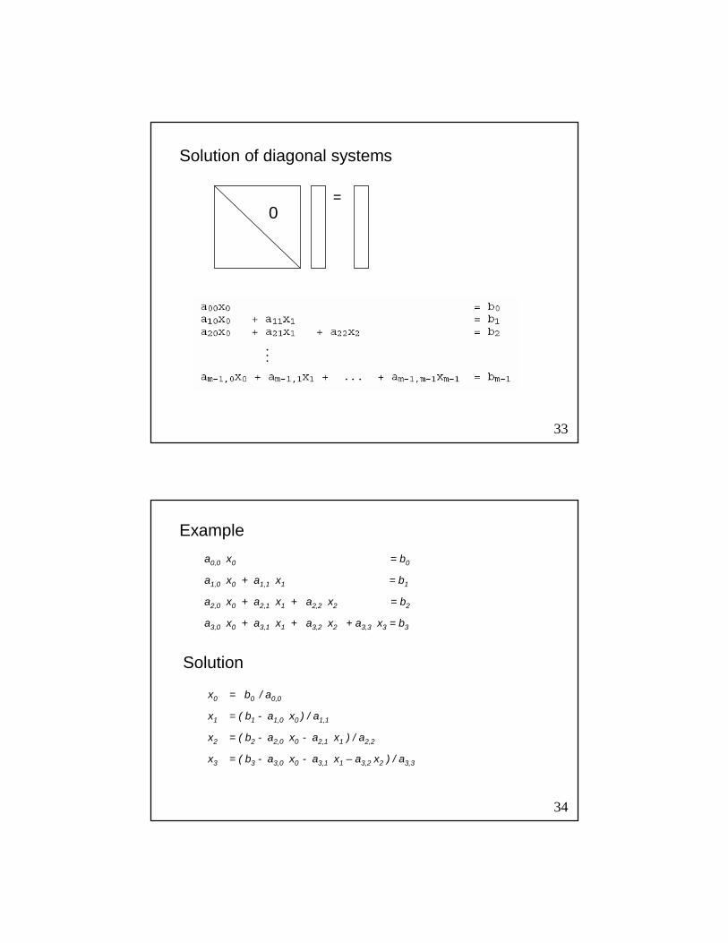
Solution of diagonal systems

=0

34

a0,0 x0 = b0

a1,0 x0 + a1,1 x1 = b1

a2,0 x0 + a2,1 x1 + a2,2 x2 = b2

a3,0 x0 + a3,1 x1 + a3,2 x2 + a3,3 x3 = b3

x0 = b0 / a0,0

x1 = ( b1 - a1,0 x0 ) / a1,1

x2 = ( b2 - a2,0 x0 - a2,1 x1 ) / a2,2

x3 = ( b3 - a3,0 x0 - a3,1 x1 – a3,2 x2 ) / a3,3

Example

Solution

35

x0 = b0 / a0,0

x1 = ( b1 - a1,0 x0 ) / a1,1

x2 = ( b2 - a2,0 x0 - a2,1 x1 ) / a2,2

x3 = ( b3 - a3,0 x0 - a3,1 x1 – a3,2 x2 ) / a3,3

36

Routing problems

• Routing a single message• Permutation routing• Multicasting and broadcasting (one to many)• Reduction or combine operations (many to one)• All-to-all broadcasting (many to many)• Personalized all-to-all (scatter-gather or gossiping)• Data packing and compaction

37

Terminology for routing problems

• Static: packets to be routed are all known before routing starts

• Dynamic: packets are created dynamically

• Off-line: routing decisions are pre-computed and stored in

routing tables

• On-line: routing decisions are computed on-line

• Oblivious: routes depends only on source and destination

• Adaptive: routes are determined based on condition of the

environment (link or node congestion, faults, delay, ….)

• Deflection routing: if shortest path is congested, use some

detour (hot potato routing).

38

Switching schemes

• Packet switching (store and forward)• Circuit switching• Wormhole switching (routing)

• Packet broken into FLITs• Buffering FLITs• Header FLIT sets a “virtual circuit”• Tail FLIT destroy the virtual circuit

• Latency for a message depends on the time to transfer (and buffer) a flit (f), the number of flits (m), as well as the number of hops (h).

• Latency is much lower than that for packet switching (depends on the time to transfer and buffer a packet (mf) and the number of hops (h).

39

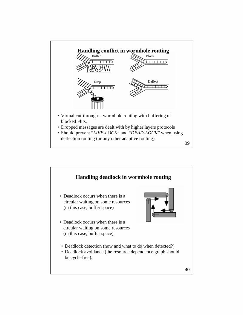
Handling conflict in wormhole routing

• Virtual cut-through = wormhole routing with buffering of blocked Flits.

• Dropped messages are dealt with by higher layers protocols• Should prevent “LIVE-LOCK” and “DEAD-LOCK” when using

deflection routing (or any other adaptive routing).

40

Handling deadlock in wormhole routing

• Deadlock occurs when there is a circular waiting on some resources (in this case, buffer space)

• Deadlock occurs when there is a circular waiting on some resources (in this case, buffer space)

• Deadlock detection (how and what to do when detected?)• Deadlock avoidance (the resource dependence graph should

be cycle-free).

41

Resource dependence graph in wormhole routing

• Buffers (at either end of a communication link) is the resource• The resource graph:

• a node for each link in the network• an edge from node i to node j if the routing allows a

message to cross link j after link i.

Routing on 2D meshes, in general, is not deadlock free.

42

Row-first routing is deadlock free

43

Deadlock free routing in meshes

If you do not want to restrict routing to “row first”, then you need to use two virtual channels for each communication links.

One link

Two buffers (one for each channel)

• A message starts on Channel 1, and moves to channel 2 when it makes a turn – If no more than one turn, then no deadlock can occur.

44

0100 0101

0110 0111

0000 0001

0010 00110

1

21100 1101

1110 1111

1000 1001

1010 1011

3

A message from a source, sq-1 , . . . , s0, to a destination xq-1 , . . . , x0 has to cross any dimension, b, for which xb ≠ sb

How many distinct routes there are between any source and destination?

Routing on a hypercube

45

0100 0101

0110 0111

0000 0001

0010 00110

1

21100 1101

1110 1111

1000 1001

1010 1011

3

When a node, nq-1 , . . . , n0, receives a message for destination node xq-1 , . . . , x0 , it executes the following• If xk = nk for k = 0, … , q-1, , keep the message

• Else { Find the largest k such that xk ≠ nk ;

Send the message to the neighbor across dimension k }

Dimension-order routing

46

Visualizing the route by unfolding the hypercube

The unfolded hypercube forms the so called “Butterfly network”

47

Semigroup operation on a hypercube (EX: global sum)

100 101

110 111

000

010 011

001

100 101

110 111

000

010 011

001

2100 101

110 111

000

010 0110

1

001

Initially: each node has a value xEach node executes the following:For j = 0 , … , q-1 do

send x to neighbor across dimension jreceive the value sent from the neighbor across dimension jx = x + the received value

Result: x in each node contains the global sum

48

010 110

011 111

000 100

001 101

Broadcasting in hypercubes

010 110

011 111

000 100

001 101

010 110

011 111

000 100

001 101

Each node executes the following: Let Ng(i) be the neighboring node across dimension i.If root, set K = q-1 ;

else if received a message from Ng(i), set K = i-1 ;For j = K , … , 0 do

send the message to Ng(j)

Broadcast on a binomial broadcast tree

493

0

1

2

0000

1000

11000100

0010 1010

0001 0011 1011

0110

0101 0111 1001

1110

1101 1111

0

3

2

1

0 0 00

2

11

000

1

time 1

time 2

time 3

time 4

50

Adaptive routing in hypercubes

= +

• Use two sets of channels (0-channels and 1-channels)• Each set of channels cannot form cycles

• A message from a source, sq-1 , . . . , s0, to a destination xq-1 , . . ., x0 has to cross any dimension, b, for which xb ≠ sb

• First, use 0-channels to cross those dimensions for which sb = 0 and xb = 1

• Then, use 1-channels to cross those dimensions for which sb = 1 and xb = 0.

51

Multistage Interconnection Networks (MINs)A modular way of building large switches from smaller switches

52

(shared memory system)Example: 16x16 switch using 32 switches organized as 4 columns of 8 switch. Each switch is a 2x2 switch.

53

Can also be used to connect processors, each with its own memory (in a distributed memory system)

54

SIMD modes (synchronized communication):

Either use message routing and synchronize processors at each step,or set the switches before sending data (circuit switching).

MIMD mode (unsynchronized communication):Use circuit switching, packet switching (without synchronization),or wormhole routing (virtual circuit switching).

Circuit-switchstates

A routing switch

buffers

55

A butterfly network(unfolded hypercube)

01

23

45

67

01

23

45

67

An Omega network(multiple shuffle/exchange)

Examples of MINs connecting 2q inputs to 2q outputs (using qstages of 2x2 switches):

01

23

45

67

01

23

45

67

56

The perfect shuffle and the exchange functions

Shuffle(xq-1 , xq-2 , … , x0) = xq-2 , … , x0 , xq-1

Exchange(xq-1 , xq-2 , … , x0) = xq-1 , xq-2 , … , x0

57

• If 2x2 switches are used to build an NxN switch (to connect Nprocessors – N being a power of 2), we need at least log Nstages.

• Number of 2x2 switches =

• If synchronous mode • Each switch is set to either cross or straight• A configuration = a specific setting of the 2x2 switches• How many possible configurations• Each configuration corresponds to a permutation (one to

one communication pattern)• A log N stage MIN cannot realize all possible permutations

(why?)

• A MIN that cannot realize all permutations is called Blocking.

58

01

23

45

67

89

1011

1213

1415

000

001

011

010

100

101

111

110

1 2 3 0 stage

The destination a3 a2 a1 a0

is coded in message header

Stage i switchai = 0ai = 1

When a message is received:Send to upper port if ai = 0Send to lower port if ai = 1

Routing in a butterfly network

59

Routing in an OMEGA network

To get from sq-1 , sq-2 , … , s0 to xq-1 , xq-2 , … , x0

• Do q shuffles• After each shuffle, do an exchange to match the corresponding

destination bit

60


000001

010

011

101

110

100

111

000001

010

011

101

110

100

111

Example: to route from source 101 to destination 110 (xor = 011)

101 011 011 110 111 111 110shuffle shuffle exchange shuffle exchange

straight cross cross

61


000001

010

011

101

110

100

111

000001

010

011

101

110

100

111

Example: to route from source 010 to destination 100 010 xor 100 = 110 = (cross, cross, straight)Route: cross at level 0, cross at level 1, straight at level 2

62

01

23

45

67

01

23

45

67

How is routing in the following OMEGA network different?

63

Capabilities of MINs for realizing arbitrary permutations:

• Blocking networks: cannot realize an arbitrary permutation without conflict -- for example, Omega can realize only nn/2 permutations.

• Non-blocking networks: can realize any permutation on-line -- for example, cross-bar switches.

• Re-arrangeable networks: can realize any permutation off-line --for example, a Benes network can establish any connection in a permutation if it is allowed to re-arrange already established connections.

The Benes network

Can be built recursively -- an nxn Benes is built from two (n/2 x n/2) Benes networks plus two columns of switches.

64

01

23

45

67

A 2x2 Benes network A 4x4 Benes network

Upper n/2 Benes

Lower n/2 Benes

01

23

45

67

65

An 8x8 Benes network

66

A 16x16 network Benes network

67

To realize a permutation (i , oi , i= 0,…, n-1) in an nxn Benesnetwork:• For each connection (i , oi ), determine whether it goes through

the upper or lower n/2 Benes.• Repeat this process recursively for each of the n/2 networks.

• Start with k=0 and (k, ok ) going through the upper Benes,• If ok shares a switch at the last column with om , then route (m,

om ) through the lower Benes.• If j shares a switch at the first column with m, then route (j, oj )

through the upper Benes.• Continue until you get an input that shares a switch with input 0.• If there are still unsatisfied connections, repeat the looping.

68

Upper n/2 Benes

Lower n/2 Benes

Example for establishing a permutation: (0,4), (4,2), (3,6), (1,0), (2,3), (6,5), (5,7), (7,1)

01

23

45

67

01

23

45

67

(0,4) upper, (6,5) lower, (7,1) upper, (1,0) lower,

(2,3) upper, (4,2) lower, (5,7) upper, (3,6) lower,

+

69

Fat tree networksEliminates the bisection bottleneck of a binary tree

70

A 16-node fat tree networks

01

23

45

67

89

1011

1213

1415

01

23

45

67

89

1011

1213

1415A fat tree networks

using 2x2 bidirectional switches

stage0 1 32

71

2x2 bidirectional switch = 4x4 uni-directional crossbar

Possible routes

Only possibilities at stage q-1

72

A fat tree networks using 4x4 bidirectional switches

01

23

45

67

89

1011

1213

1415

01

23

45

67

89

1011

1213

1415

Routing in a fat tree- multiple paths- un-equal path lengths

73

01

23

45

67

89

1011

1213

1415

Routing in a fat tree

stage0 1 32

source sq-1 , sq-2 , … , s0

destination xq-1 , xq-2 , … , x0

-Find smallest k such that si = xi , i=k+1,…,q-1(if no such k exists, then k = q-1 )

- Route arbitrarily up the tree to a switch in stage k- Route down the tree as follows:

at stage i, i= k, … , 0

if xi = 0, route to upper portelse route to lower port

Examples (q = 4):0011 1110 (k = 3)1000 1100 (k = 2)

74

qxq

qxq

qxq

qxq

pq inputs

qxq

qxq

qxq

qxq

pxp

pxp

pxp

pq outputs

A Clos network (shown for p = 4)

q switchp switch p switch

75

Embedding task graphs into processors

76

Embedding a logical topology into a physical topology

Embedding = node mapping + edge mapping

Embedding a seven-node binary tree in 2D meshes of various sizes

77

Properties of embeddings

Dilation: length of the longest path to which a logical edge is mapped

Load Factor: maximum number of logical nodes mapped onto one physical node

Congestion: maximum number of logical edges mapped onto one physical edge

In the examples in the last slide3x3 2x4 2x2

1 2 1

1 2 2

1 1 2

9/7 8/7 4/7Expansion: ratio of the number of nodes

in the two topologies

Why is each of the above factors important?

78

100 101

110 111

000 001

010 011

00 01

1110

0

1

0

1

2

0100 0101

0110 0111

0000 0001

0010 00110

1

21100 1101

1110 1111

1000 1001

1010 1011

3

Embedding a linear array into a hypercube

79

Binary Gray code (Hamming distance between any two code words = 1)

01

0110

0011

0001111010110100

00001111

000001011010110111101100100101111110010011001000

0000000011111111

80

Embedding a 2D array into a hypercube

1,3 1,2

1,0 1,1

0,3 0,2

0,0 0,1

2,3 2,2

2,0 2,1

3,3 3,2

3,0 3,1

0,0 0,1 0,2 0,3

1,0 1,1 1,2 1,3

2,0 2,1 2,2 2,3

3,0 3,1 3,2 3,3

Theorem: we can embed a 2a x 2b

array into a (a+b)-dimensional hypercube with dilation 1.

81

Embedding a complete binary tree into a hypercube

100 101

110 111

000 001

010 011

Theorem: we cannot embed a 2q -1 complete binary tree in a q-dimensional hypercube with dilation 1.

Proof: first divide the nodes in the cube to odd nodes (those with an odd number of 1’s in the address) and even nodes (those with an even number of 1’s in the address). To preserve unit dilation when embedding the tree, more than half the nodes need to be even (or odd) nodes. This is not possible.

82

Embedding a double rooted tree into a hypercube

100 101

110 111

000 001

010 011

Theorem: we can embed a 2q double-rooted complete binary tree in a q-dimensional hypercube with dilation 1.

000

010

110

101

011 001 111

100

Will not provide a general proof but will give you an example for the embedding in the case of 8 nodes.

Note: embedding a double-rooted tree with dilation 1 is equivalent to embedding a sinngle rooted tree with dilation 2.

83

Cache coherence in SMP’s

84

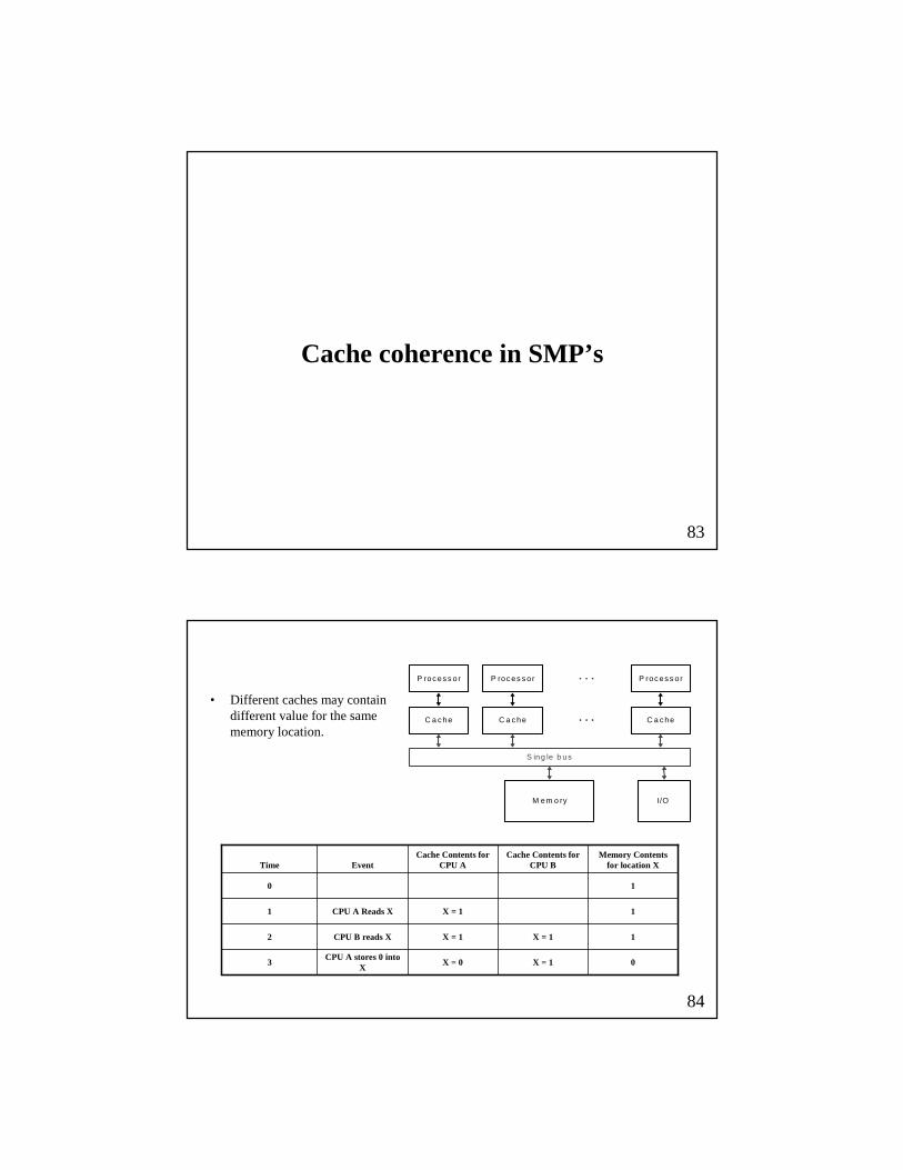
• Different caches may contain different value for the same memory location.

C a c he

P roc es s o r

C a c he

P roc es s o r

C a c he

P roc es s o r

S ing le b us

M em o ry I/O

0X = 1X = 0CPU A stores 0 into

X3

1X = 1X = 1CPU B reads X2

1X = 1CPU A Reads X1

10

Memory Contents for location X

Cache Contents for CPU B

Cache Contents for CPU AEventTime

85

Approaches to cache coherence

• Do not cache shared data

• Do not cache writeable shared data

• Use snoopy caches (if connected by a bus)

• If GMSV not connected by a bus or DMSV (physically distributed memory), then need another solution – directory-based protocols.

86

Snooping cache coherence protocols

• Each processor monitors the activity on the bus

• On a read miss, all caches check to see if they have a copy of the requested block. If yes,they supply the data (will see how).

• On a write miss, all caches check to see if they have a copy of the requested data. If yes, they either invalidate the local copy, or update it with the new value.

• Can have either write back or write through policy.

Cache tag�and data

Processor

Single bus

Memory I/O

Snoop�tag


Processor

Snoop�tag


Processor

Snoop�tag

87

Example: Write Invalidate

00Cache Miss for XCPU A Reads X

111Cache Miss for XCPU B Reads X

01Invalidation for XCPU A writes 1 to X


0


Cache Contents forCPU B

Cache Contents for CPU ABus ActivityProcessor Activity

88

Example: Write update

00Cache Miss for XCPU A Reads X

111Cache hit for XCPU B Reads X

111update for XCPU A writes 1 to X


0


Cache Contents forCPU B

Cache Contents for CPU ABus ActivityProcessor Activity

89

An Example Snoopy Protocol

• Invalidation protocol, write-back cache

• Each block of memory is in one state:

– Clean in all caches and up-to-date in memory (Read-Only),

– Dirty in exactly one cache (Read/Write), OR

– Not in any caches

• Each cache block is in one state:

– Shared : block can be read (clean, read-only)

– Exclusive : cache has only copy, its writeable, and dirty

– Invalid : block contains no data

• Read misses: cause all caches to snoop bus

• Writes to clean blocks are treated as misses -- invalidates all other caches

90

Snoopy Cache State Machine (CPU Events)

InvalidShared

(read only)

Exclusive

(read/write)

CPU read missPlace read miss

on bus

CPU read missPlace read miss on bus

CPU read m

iss

Write back block

CPU write (h

it or m

iss)

Place write m

iss on bus

and write back re

placed block

CPU write missPlace write miss on bus and write back

replaced block

CPU write missPlace write miss on bus

Note: A read hit does not change the state.

CPU write hit

91

Snoopy Cache State Machine (Bus Events)

InvalidShared

(read only)

Exclusive

(read/write)

Write miss (or invalidate) for this block

Read miss fo

r this block

Write-back block;

Write miss for this block

Write-back block

92

• Assumes A1 and A2 map to same cache block B.• Initial cache state is invalid

P1 writes 10 to A1

P1 reads A1

P2 reads A1

P2 write 20 to A1

P2 writes 40 to A1

B = invalid

A1 = 10 (exclusive)

A1 = 10 (exclusive)

A1 = 10 (shared)

B = invalid

B = invalid

B = invalid

B = invalid

B = invalid

A1 = 10 (shared)

A1 = 20 (exclusive)

A2 = 40 (exclusive)

In P1’s cache In P2’s cacheEvent

Example

93

Directory-based coherence protocols

• For shared address space over physically distributed memory• A controller decides if access is Local or Remote • A directory that tracks state of every block in every cache (dirty, clean, …)• Info per memory block vs. per cache block?

• PLUS: In memory => simpler protocol (centralized/one location)• MINUS: In memory => directory is ƒ(memory size) vs. ƒ(cache size)

• With each block in each memory keep a state:• Shared: cached in one or more processors, and memory is up-to-date• Uncached: no processor has it; not valid in any cache)• Exclusive: 1 processor (owner) has data; memory out-of-date

• In addition to the state, must track which processors cached the block• The owner (home) of each block in a cache is stored with the block.

94

Directory protocols

• No bus and don’t want to broadcast:• interconnect no longer single arbitration point• all messages have explicit responses

• Keep it simple(r):• Processor blocks until access completes• Assume messages received and acted upon in order sent

• Typically 3 processors involved• Local node where a request originates• Home node where the memory location of an address resides• Remote node has a copy of a cache block

• Example messages on next slides: P = local node, H = home node, A = address (block)

95

Directory Protocol Messages

Message type Source Destination Msg Content

Read miss P H P, AIf A is shared or uncached, H sends “data (P,A)” message and sets State(A) = shared,If A is exclusive at another processor R, H sends “Fetch (P,H,A)” message to R

Write miss P H P, AIf A is uncached, H sends A to P and sets State(A) = exclusiveIf A is shared, H sends A to P, H sets State(A) = exclusive and send “Invalidate A” to every remote

cache, R, sharing A,If A is exclusive at another processor R, H sends “Fetch (P,H,A)” message to R

Invalidate H Remote node, R AR invalidates A in its cache.

Fetch H Remote node, R P,H,AR fetches A and sends “data(P,A)” and “data(H,A)”, and Invalidates A in local cache of R

data a processor P P,AA message containing the data in A

evolution of parallel hardware

Documents