AIRTIME TRANSFERS AND MOBILE COMMUNICATIONS:

EVIDENCE IN THE AFTERMATH OF NATURAL DISASTERS∗

Joshua Blumenstock, University of WashingtonNathan Eagle, Santa Fe Institute

Marcel Fafchamps, Oxford University

December 31, 2015

Abstract

We provide empirical evidence that Rwandans use the mobile phone network to transfer airtime tothose affected by unexpected shocks. Using an extensive dataset on mobile phone activity in Rwandaand exploiting the quasi-random timing and location of natural disasters, we show that individuals maketransfers and calls to people affected by disasters. The magnitude of these transfers is small in absoluteterms, but statistically significant; in response to the Lake Kivu earthquake of 2008, we estimate thatroughly US$84 in airtime was transferred to individuals in the affected region, that 70% of these transferswere immediately used to make outgoing calls, and that US$16,959 was spent calling those near the epi-center. Unlike other forms of interpersonal transfers, mobile airtime airtime is sent over large geographicdistances and in response to covariate shocks. Transfers are more likely to be sent to wealthy individuals,and are sent predominantly between pairs of individuals with a strong history of reciprocal favor exchange.

JEL Classification: O17, H84, O16, O33

∗The authors are grateful for thoughtful comments from Alain de Janvry, Stefano DellaVigna, Frederico Finan, MauricioLarrain, Ethan Ligon, Jeremy Magruder, Edward Miguel, Alex Rothenberg, Elisabeth Sadoulet, and seminar participants atNEUDC, PACDEV, MWIEDC, and the Berkeley Development Lunch. We gratefully acknowledge financial support from theInternational Growth Center, the National Science Foundation, the Institute for Money, Technology and Financial Inclusion,and the NET Institute. All errors are our own.

1

1 Introduction

In the aftermath of unexpected economic shocks, people often rely on friends and family for support in

cash and in kind. In developing countries, support has historically been limited by weak infrastructure for

communicating with and assisting others. As a result, most empirical evidence indicates that assistance and

favors are primarily exchanged within small, geographically-defined communities (Udry 1994, Fafchamps &

Gubert 2007, de Weerdt & Fafchamps 2010).

In recent years, the proliferation of mobile phones and of phone-based financial services has provided

billions of individuals in developing countries with a new mechanism for communication and interpersonal

transfers. With roughly 250 deployments in the global south, such “branchless banking” systems allow

individuals to transfer money from one phone to another at a fraction of the cost of existing alternatives

(McKay & Pickens 2010, GSMA 2014). In Kenya, for instance, where over US$200 million is transferred

over the system per day, individuals with access to the mobile money network are better able to smooth

consumption than those without (Suri et al. 2012, Jack & Suri 2014, Pulver 2009).

We exploit a novel source of data on mobile phone use to better understand how individuals use the

mobile phone network to cope with unexpected shocks. We observe the entire universe of mobile phone-

based communications in Rwanda from 2005 through 2009, including transaction logs that contain detailed

information on millions of interpersonal transfers of mobile airtime and billions of phone calls. Our primary

results are identified by a magnitude 6.0 earthquake in the Lake Kivu region of Rwanda, which left 43 dead

and 1,090 injured, and caused significant disruption in public utilities and other local infrastructure. While

Rwanda did not have a functioning mobile money system at the time of this earthquake, we observe that

in the earthquake’s immediate aftermath, individuals living across Rwanda transferred airtime and initiated

phone calls to individuals living close to the epicenter. We estimate that an additional US$84 in airtime

was transferred, and that US$16,959 was spent making phone calls, to affected individuals. The economic

significance of the airtime transfers was thus modest, though this is due in part to the fact that only 1,400

individuals in the region had ever used the airtime transfer service prior to the earthquake, creating a small

population of potential recipients. The value of the phone calls was much higher, though more difficult to

interpret. Since in Rwanda the caller bears the full cost of making a phone call, this may represent an

implicit transfer of communication costs, but more likely it simply expresses the desire of the calling party

to communicate in a time of crisis. Our empirical results are robust to the inclusion of dyad fixed effects,

time dummies, and time-varying controls. We further provide several robustness checks and placebo tests

to show that the results are not simply driven by the large number of observations in our dataset.

Our analysis reveals significant heterogeneity in the nature of transfers sent in response to unexpected

2

shocks. Using several different proxies for socioeconomic status based on follow-up interviews with a rep-

resentative sample of mobile phone subscribers, we find that while wealthier individuals are more likely to

recieve transfers under normal circumstances, they are even more likely to receive transfers after natural

disasters. The recipients of shock-induced transfers also have larger social networks, and are more centrally

positioned within their network. Along several additional dimensions, it is the historically privileged strata

of Rwandan society who appear to benefit most from access to mobile phone-based transfers.

Finally, we analyze the pattern of interpersonal transfers to shed light on the motives that cause people to

make transfers to those impacted by covariate shocks. Our goal is to test whether the observed transfers are

more consistent with a model of giving based on pure charity (Becker 1974, Andreoni & Miller 2002) or with a

model of conditional reciprocity where individuals give because they wish to receive in the future (e.g., Ligon

et al. 2002, Foster & Rosenzweig 2001, Falk & Fischbacher 2006). While our ability to cleanly differentiate

between these models is limited by the observational data at our disposal, three stylized facts in our data

appear broadly consistent with a model based on reciprocity. First, there is a strong history-dependence of

transfers sent in response to large shocks, in that after the earthquake people are more likely to send funds

to people from whom they have received in the past. Second, it is the wealthier individuals who receive

the largest volume of transfers in the immediate aftermath of the earthquake, not the poorer individuals

that one would expect in a naive model of charity. Third, post-quake transfers decrease with the geographic

distance between individuals, even when controlling for social distance and unobserved, time-invariant dyadic

heterogeneity.

To summarize, the evidence indicates that Rwandans use airtime transfers to help each other cope with

large economic shocks, that benefits from these transfers are not uniformly distributed, and that the pattern

of transfers is consistent with conditional reciprocity. To the extent that airtime transfers can be interpreted

as a form of favor exchange, there are two features that distinguish the mobile phone-based response from

much of the evidence on favor exchange, especially traditional risk sharing. First, whereas traditional risk

sharing networks are constrained by geography (Udry 1994, Fafchamps & Gubert 2007), transfers sent over

the mobile phone network are sent over large distances, often in excess of 100km. Second, these transfers are

sent in response to large, covariate shocks, rather than the geographically isolated, idiosyncratic shocks that

are the focus of much of the existing risk sharing literature (Townsend 1994, De Vreyer et al. 2010, Gine &

Yang 2009).

These findings complement recent work by Jack & Suri (2014), who use consumption data to show that

Kenyans with access to mobile money are better able to smooth consumption than those without. It also

relates closely to a growing body of research concerned with understanding the economic impact of mobile

phones and other information and communication technologies (ICTs) in developing economies. Recent work

3

in this area describes how mobile phones can, under certain conditions, reduce information asymmetries and

search costs in agricultural markets (Jensen 2007, Aker 2008, Fafchamps & Minten 2012, Aker & Fafchamps

2014), lower transaction costs (Jack & Suri 2014), and potentially provide an alternative device for savings

(Mbiti & Weil 2011, Mas & Mayer 2011, Blumenstock et al. 2015).

We make two methodological contributions that we hope can help facilitate the use of large-scale, network-

based datasets in applied microeconomic and development research. First, we develop an approach to

inferring the relative wealth of mobile phone subscribers from their history of mobile phone use. The sole

purpose of this approach is to proxy for the relative wealth of transfer recipients at a particular point in

time. Second, we develop an algorithm for locational inference that allows us to continuously impute the

location of an individual based on her intermittent sequence of phone calls. We use this method to determine

whether or not a subscriber is affected by a regional disaster, but the algorithm could be implemented more

broadly to identify individuals in need of help.

2 Background and Context

The context for our study is Rwanda, a small, landlocked nation of 10 million people, where roughly 90%

of the population survives on subsistence agriculture. We focus our analysis on the period from 2005-2009,

a period during which mobile phone penetration increased from roughly 2.5 percent to 33.4 percent – a

compound annual growth rate of roughly 74 percent. Such rapid growth has been common in many sub-

Saharan African nations, where landlines are rare and the cost of owning a mobile phone is falling quickly.

The cost of mobile telephony during this period represented a significant portion of household expenditures

(Ureta 2005). At the time of our study in Rwanda, it cost roughly $50 for the phone, and an additional $0.20

per minute and $0.10 per SMS (Republic of Rwanda 2010, Donner 2008). The ITU estimates the monthly

“price basket” for mobile service was $12.30 per month, or $147.60 per year, which represented a significant

portion of the PPP-adjusted GDP per capita of $800.1

Our empirical analysis focuses on interpersonal transfers of airtime funds between mobile subscribers.

These transfers were made possible by a rudimentary precursor to “mobile money” that was launched in

Rwanda in late 2006 by the monopoly mobile phone operator at the time. In Rwanda, where nearly all

phone usage is prepaid and all incoming calls are free, the system works much like a debit card. To make

a transfer, individuals buy airtime scratch-cards, ranging from US$0.10 to US$20, from thousands of stores

and street vendors throughout the country. The purchased balance is deposited on the prepaid mobile phone

1The price basket is based on the prepaid price for 25 calls per month spread over the same mobile network, other mobilenetworks, and mobile to fixed calls and during peak, off-peak, and weekend times. The basket also includes 30 text messagesper month (http://devdata.worldbank.org/ict/rwa_ict.pdf).

4

account, and can then be used to make phone calls, to send text messages, or to use other mobile services.

Using the transfer service, one subscriber can transfer an arbitrary balance, instantaneously and free of

charge, to another subscriber. The transferred balance can then be used by the recipient to make calls, or

re-transferred to another subscriber or vendor. During the period of time we analyze (2005-2009), there was

no formal “cash-out” policy that guaranteed that the recipient could resell airtime to a vendor, but informal

cashing-out was commonplace, with vendors typically charging 10-20% for the transaction.2 In 2010, the

phone company launched a fully fledged mobile money service that, among other features, made it possible

to cash out airtime at fixed tariffs.

In the past several years, similar systems have become popular in developing countries, where over

1.7 billion people own a mobile phone but do not have a bank account (CGAP and GSMA 2009). The

airtime transfer service we focus on was a common antecedent to most modern mobile money deployments

(Aker & Mbiti 2010). Compared to alternative mechanisms for sending money available to Rwandans,

sending airtime was considerably cheaper, faster, and more convenient (Table 1). Other options included

MoneyGram, Western Union, or the Post Office, but transaction costs across these services ranged from

10 - 100% and, at the time of our study, none of these services permitted a transfer of less than US$10.

Rwandans could also send money through a bus or taxi driver, but these transfers were contingent on bus

schedules and road conditions – and much slower than airtime transfer.

3 Identification and Estimation Strategy

3.1 The giving response to unexpected shocks

The focus of our empirical analysis is on airtime transfers sent in response to unpredictable but publicly

observed shocks such as earthquakes and floods. We also quantify the volume and value of calls made in

response to such shocks. Empirically, we use spatial and temporal variation to identify individuals who are

affected by these shocks, then measure how airtime transfers and communication events respond to these

unexpected events. The response can be measured at three levels. We start at the regional level, to measure

the total response to the shock. We then disaggregate transfers to the level of the individual sender and

receiver, to study heterogeneity in who sends and receives. Finally, we disaggregate the analysis to the level

of the dyad, which permits us to analyze the types of relationships that are likely to be involved in transfers,

and to informally test between competing models of giving.

2Based on conversations with Rwandan informants at the time. In a 2009 survey of 910 Rwandans, respondents were askedto list “the preferred method for sending money to a friend or family member.” 28 percent listed “Airtime Transfer” as theirpreferred method (Blumenstock & Eagle 2012). This suggests that, prior to 2010, mobile airtime was perceived as relativelyliquid.

5

Formally, let τijrt denote the gross transfer of airtime (or the total value of the call) sent to an individual

i, located in region r at time t, from another individual j. Further define τirt =∑

j τijrt the total gross

transfers received by user i in region r at time t, and define τrt =∑

i τirt as the total gross transfers received

by users in location r at time t. When analyzing calls instead of airtime transfers, τijrt is the value of airtime

spent by j in communicating with i. We estimate models of the form:

τrt = α1 + γ1Shockrt + θt + πr + εrt (1)

τirt = α2 + γ2Shockirt + ϕNearEpicenterit + θt + πi + εirt (2)

τijrt = α3 + γ3Shockirt + ϕNearEpicenterit + θt + πij + εijrt (3)

where Shockrt is a dummy variable equal to 1 if location r received a shock at time t, and Shockirt equals 1

if t is the day of a shock and i was in an affected region r at that time. NearEpicenterit takes the value 1

at all times when i is near the epicenter of the shock (irrespective of a shock occurring), and controls for the

possibility that individuals might receive transfers when visiting the shock-prone regions. Time dummies

θt control for long-term growth in traffic, as well as day-of-the-week (e.g., week-end) and day-of-the-month

(e.g., payday) effects that affect all regions similarly. Location and recipient fixed effects πr and πi control

for the fact that different regions and individuals are more likely to receive transfers on average. Dyadic fixed

effects πij control for the average intensity and direction of transfer flows between two individuals. Finally,

to minimize the likelihood that our results are driven by differential growth in mobile usage across locations,

we restrict the analysis to a specific time window Tmin ≤ ts ≤ Tmax around the time of the shock ts.

Identification is achieved as in a difference-in-difference framework: parameters γ1, γ2 and γ3 represent

the average treatment effect of the shock on people with access to the mobile network. The exogeneity

of Shockrt is guaranteed if its timing could not have been predicted, i.e., the shock constitutes a natural

experiment. If γ1 > 0, γ2 > 0 and γ3 > 0, this is interpreted as evidence that the shock Shockrt caused

an increase in airtime transfers to users in the affected region. We check the robustness of our results in

various ways, notably by varying the time window over which the models are estimated, by controlling for

several factors that depend on both time and location, and by running a number of falsification and placebo

tests. Following Bertrand et al. (2004), in individual and dyadic regressions standard errors are clustered by

location (i.e., by the location of the nearest cellular tower).

6

3.2 Heterogeneity in transfers

To better understand the nature of the response to shocks, we allow for heterogeneous effects for different

types of individuals and for different types of dyadic sender-recipient pairs. We denote these individual and

dyadic characteristics by Zi and Zij , respectively. As discussed in greater detail in the next section, relevant

Zi include i’s wealth and social connectedness, and Zij include the geographic distance between i and j, and

information about the history of transfers between i and j. Heterogeneity is then esimated using models of

the form:

τit = α2+ γ2Shockit + β2ZiShockit + ϕ2NearEpicenterit +

η2ZiDayOfShockt + ζ2ZiNearEpicenterit + θt + πi + εit (4)

τijt = α3+ γ3Shockit + β3ZijShockit + ϕ3NearEpicenterit +

η3ZijDayOfShockt + ζ3ZijNearEpicenterit + θt + πij + εijt (5)

As before, τijrt denotes the gross transfer of airtime received by an individual i, located in region r at

time t, from another individual j, with τirt =∑

j τijrt. Shockit takes the value 1 if i is affected by the shock

and zero otherwise, and is the product of DayOfShockt, a dummy variable taking the value one on the day

of a severe shock and NearEpicenterit, a dummy variable indicating whether i was close to the shock on day

t. Double interaction terms of the form ZiDayOfShockt are included to control for the possibility that, in

the country as a whole, variation in Zi affects transfers on the day of the shock differently from other days.

Our primary interest is in the estimates of β2 and β3, which indicate the types of individuals and dyads that

are most likely to receive transfers caused by economic shocks.

4 Data and Measurement

The main dataset we use comes from Rwanda’s primary telecommunications operator, which held a near

monopoly on mobile telephony until 2009.3 The data contain a comprehensive log of all activity that occurred

on this network between early 2005 and early 2009. In total, we observe detailed information on over 50

billion transactions (including calls, text messages, and airtime transfers and purchases), covering roughly 1

million subscribers over four years. Summary statistics of this dataset are provided in Table 2.

Our empirical analysis focuses on interpersonal transfers of airtime credit sent between one mobile sub-

scriber and another. In our dataset, we observe detailed information on roughly 10 million such transfers. As

3During the window of time we examine, the operator we focus on maintained over 90% market share of the mobile market.The company’s primary competitor did not gain traction in the market until the end of 2008, and only in 2010 did the marketbecome competitive. The number of landlines in Rwanda is negligible (roughly 0.25% penetration).

7

shown in Figure 3, the system was not heavily utilized prior to 2008, when the operator launched a nation-

wide promotion and uptake dramatically increased. We focus on transactions sent prior to this growth stage.

For each transaction, we observe the date, time, and value of the transfer, as well as a unique (anonymized)

identifier for both the sender and recipient. To estimate the regressions described in sections 3, we aggregate

this raw data on each day for each region (equation 1), individual (equation 2), and dyadic pair of individuals

(equation 3). This allows us to measure, at three different levels of aggregation, the net and gross volume of

airtime received on each day.

4.1 Physical Location

The identification strategy we employ relies on spatial, as well as temporal, variation in transfers. Therefore,

it is important that we be able to assign each individual, on each day, to an approximate geographic location.

In standard GSM cellular networks, such as the one in place in Rwanda, the phone company does not record

continuous GPS coordinates of each subscriber. However, each phone call in the database is tagged with an

originating and terminating tower, which allows us to roughly place the caller and recipient at the time of

the call.

We use these discrete events to approximate the continuous trajectory of each user through time and

space, based on the intermittent sequence of phone calls logged by the mobile operator. As can be seen

in Figure 1, which shows the spatial distribution of cell phone towers in early 2008, towers in rural areas

are relatively sparse, with a median distance between towers of 68km. The locational inference algorithm

employs a smoothing function K(·) to predict the unknown location of i at time t from the kernel-weighted

Euclidean centroid of i’s known locations at times in the vicinity of t (see Figure 2).

Formally, we estimate the unknown location rit of individual i at time t as

rit =1

Nit

Tmax∑s=Tmin

K(t− s

h) · qis

where Nit is the total number of phone calls made by i within a window of time [Tmin, Tmax] around t,

and qis is the (known) location of the tower used at time s. The kernel K(x) is a symmetric function that

integrates to one, which specifies the extent to which additional weight is placed on calls close in time to

t. In our results we use a uniform kernel such that K(u) = 1/Ni, however very little changes if a different

kernel is specified.

8

4.2 Characteristics of individuals and dyads

To estimate our heterogeneous effects models, we require characteristics of individuals (Zi) and dyads (Zij).

Many of these can be computed directly from the anonymized call records dataset, including the following:

• Physical distance between i and j (Dijt): To estimate the distance between i and j at time t, we

first compute the (latitude,longitude) locations rit = (ϕi, λi) and rjt = (ϕj , λj) using the locational in-

ference algorithm described in Section 4.1. Then, we compute the arc distance Dijt using the haversine

formula:

Dijt = 2r · arcsin

(√sin2

(∆ϕ

2

)+ cosϕi cosϕj sin

2

(∆λ

2

))

where ∆ϕ = |ϕi − ϕj |, ∆λ = |λi − λj | and r = 6356.78 is the radius of the earth.

• Social connectedness (Sij): To measure the strength of the social connection between i and j, we

calculate Sij in two ways: first, following Marmaros & Sacerdote (2006) we count the total number

of non-monetary interactions (phone calls and text messages) between i and j in a 3-month window.

Second, as in Karlan et al. (2009), we measure the maximum network flow as the number of distinct

paths between i and j in the complete undirected call graph.

• Past transfer history (Tijt): Since we observe all transactions between i and j over a 4-year period,

it is possible at any point t to compute the gross balance of payment sent from j to i as Tijt =∑

s<t τijs

and from i to j as Tjit =∑

s<t τjis. The net balance of transfers Tnetijt is simply Tijt − Tjit.

• Individual Characteristics (Zi): In addition, we compute a large number of characteristics that

are summarized for the survey sample in Appendix Table 7, including:

– Total expenditures on airtime: The amount spent on making calls and sending text messages.

– Days of activity : The number of different days on which the phone was used.

– Call activity : Number of outgoing and incoming calls. We separately looking at outgoing and

incoming calls, outgoing and incoming text messages, and international call activity.

– Degree: Number of unique contacts with whom the person communicates.

– Clustering : Percentage of first-degree contacts that have contacted each other.

– Betweenness: Average shortest path between the user and 50 randomly sampled numbers.

4.3 Inferred socioeconomic status

In assessing heterogeneity in mobile phone-based activity, we are interested in understanding the extent to

which wealthier or poorer individuals are more likely to receive interpersonal transfers following economic

shocks. However, since our data are anonymized and contain no demographic or economic characteristics, we

9

do not directly observe the socioeconomic status (SES) of individual subscribers. Yet, wealthy individuals

tend to have different communication patterns than poorer individuals, and there is good reason to suspect

that mobile phone use is highly correlated with SES (Blumenstock & Eagle 2012). For instance, we observe

that wealthy people tend to make a larger number of international calls, poorer individuals tend to receive

more calls than they make (because only the caller pays for the cost of the call in Rwanda), and poorer

individuals tend to buy airtime in smaller denominations. Thus, we construct a composite indicator of SES

that indicates the predicted wealth of each mobile phone subscriber, where the prediction is based on the

subscriber’s anonymous history of calls. We briefly summarize this approach here, and discuss in much

greater detail the limitations of this approach, as well as a number of robustness checks that we run to test

the validity of this method, in Section (iv).

1. Rwandan Household Survey (RHS): We use a nationally representative household survey conducted

by the Rwandan government in 2005 on a representative set of 6,900 households. The survey contains

roughly five hundred questions typical of Living Standard and Measurement Surveys, and includes a

detailed module on demographic composition and socioeconomic status (National Institute of Statistics-

Rwanda 2007). Most relevant to the current analysis, roughly seventy questions were asked about asset

ownership and household expenditures, which makes it possible to estimate each household’s annual

expenditures in a manner following Deaton & Zaidi (2002).

2. Phone survey conducted by authors: In 2009, we conducted a phone survey of a geographically stratified

group of Rwandan mobile phone users. Using a trained group of enumerators from the Kigali Institute

of Science and Technology (KIST), a short, structured interview was administered to roughly 1,000

individuals. In the phone survey, we collected answers to a small subset of the RHS questions (described

above) about household asset ownership and housing characteristics. The survey instrument contained

a maximum of 80 questions and took between 10 and 20 minutes to administer. Complete details on

the administration of this phone survey are provided in Blumenstock & Eagle (2010).4

4Most relevant to this paper, the survey population was designed to be representative sample of active phone users. Startingwith a population of 800,000 active subscribers (in 2009), each individual was assigned to a district based on the locationfrom which the majority of his or her calls were made. We then randomly sampled 300 numbers from each of 30 districts,creating a base survey population of 9,000 candidate respondents. Our survey team called roughly 10 percent of this candidatepopulation. Conditional on the responding picking up the phone, response rates were extremely high (98%); however, roughly38% of respondents never picked up the phone, even after three attempts were made. To correct for non-response, samplingweights for each district were determined based on the distribution of districts in the set of 800,000 active numbers, and surveyweights are assigned to make the proportion of respondents equal to the proportion of active phone users in each district.

However, as discussed in greater detail in Blumenstock & Eagle (2010), there are only modest differences between the groupof individuals who participated in the phone survey and those who did not. There is a large and significant difference in thenumber of days during which the phone is used (likely driven by the fact that many of the non-respondents have switched SIMcard), but there are not statistically signficant differences in the level of activity per day in which the phone is active (includingcalls per day, SMS per day, degree centrality, total airtime purchases, etc.).

10

Utilizing these data, we follow a 3-step process to model the relationship between phone use and wealth,

wherein we (i) use the Rwandan RHS data to model the relationship between annualized expenditures and

assets; (ii) use the asset-based questions from the phone survey to create a measure of predicted annualized

expenditures for this sample; and (iii) merge the call records from this sample with the predicted annualized

expenditures to model the relationship between SES and phone use. These steps are explained in greater

detail below.

(i) Modeling the relationship between assets and expenditures:

Using a nationally-represenative Rwandan Household Survey (RHS) that contains detailed consumption and

expenditure information (National Institute of Statistics-Rwanda 2007), we first estimate a hedonic regression

of annual expenditures Yid of household i in district d on fixed assets Aid and housing characteristics Hid.

Yid = α+

hmax∑j

βjHid +

amax∑k

δkAid + µd + ϵid (6)

The quantities Yid, Aid, and Hid are all captured in the RHS, and µd is a district fixed effect. Equation

(6) predicts the annual expenditure Yid of a household on the basis of observable Aid and Hid. This is

conceptually similar to a proxy-means test (cf. Montgomery et al. 2000), wherein we regard Yid is as a

proxy for permanent income. Appendix Table 6 gives the coefficients from the linear terms that result from

estimating (6). It is evident that annual expenditures are heavily correlated with asset ownership.5

(ii) Predicting the expenditures of phone survey respondents:

After estimating (6) on the RHS data, we obtain a vector of coefficients βj and δk that can be used to

predict total expenditures given knowledge of assets and housing characteristics Aid and Hid. Thus, for any

individual in Rwanda, we could in principle predict that individual’s annual expenditures, denoted by Yid,

by asking that individual a small number of questions about his household. In our case, we conducted the

phone survey described above in which, for each surveyed individual, we collected a limited set of Hid and

Aid through a short, phone-based instrument. The questions included in this survey were those where we

observed a significant unconditional correlation with annualized expenditures in the RHS data, and where

our piloting indicated that a reliable response could be obtained over the phone.6 Using the Hid and Aid

5To reduce the potential bias of outliers, we remove outliers with abnormally large studentized residuals, following a standardprocess described in (Fox 1997). However, our results change very little if we use an alternate technique for removing outliers,such as removing the top 1% or 5% of extreme values.

6We found that several questions which were highly predictive of annual expenditures in the RHS data were not well-suitedto a phone-based survey. For instance, in pilot surveys our ennumerators found that consumption and expenditure moduleswere time consuming and reported low confidence in respondents’ answers. Other questions, such as the amount of land ownedby the respondent, yielded noisy responses with inconsistent units of measurement, and seemed likely to yield non-traditional

11

collected through the phone survey, we than calculate the predicted annual expenditures Yid for each phone

survey respondent using the coefficient estimates from equation (6).

(iii) Predicting predicted expenditures of full population of mobile phone subscribers:

Using the above technique, it is possible to obtain the predicted expenditures Yid for each of the individuals

contacted in the phone survey. We then compute, for each phone user, a vector of phone usage variables

Xir thought to be correlated with income, such as the total number of calls made and the average amount

of airtime purchased over a given time interval. A subset of these variables are reported for the sample of

phone survey respondents in Appendix Table 7. We then fit a flexible model of the form:

Yid = f(Xir) (7)

and estimate f(.) using data from the phone user survey. In estimating equation (7) we exclude all data on

interpersonal transfers from Xir to help reduce potential endogeneity when estimating heterogeneous effects

models (4) and (5), where τijt is the dependent variable. Instead, Xir consists primarily of characterstics

of each subscriber’s history of phone calls, text messages, airtime purchases, and social network structure.

Appendix Table 8 presents the results from regressing predicted expenditures on several metrics of phone

use, polynomial (squared) terms, and district fixed effects.

In the heterogeneous effects specifications that rely on a measure of individual SES, we use the predictedY id obtained by applying the estimated flexible function f(.) to the full sample of 1.5 million phone users.

This particular metric is not intended to be externally valid to the at-large population, for indeed there are

significant differences in the wealth distribution of mobile phone owners and non-owners (Blumenstock &

Eagle 2010). Instead, it is intended to estimate whether the mobile phone owners receiving transfers are

wealthy or poor relative to other mobile phone owners. We discuss alternate measures of SES in Section (i),

and concerns about the potential endogeneity of these measures in Section 6.2 (iv).

5 Results

Our identification strategy requires a shock (Shockrt) that is exogenous to mobile phone activity. The

primary shock that we exploit is a large earthquake that occurred in the Western Rusizi and Nyamasheke

districts of Rwanda on February 3, 2008. The magnitude 6 earthquake left 43 dead and 1,090 injured. It

destroyed 2,288 houses and caused regional school closures and electrical outages (though only one cell tower

measurement error. As calls to respondents were billed per second, and given limited survey resources, we sought a balancebetween predictive power and perceived reliability.

12

of 267 was affected). The effects of the earthquake, though large, were geographically contained. The United

States Geographical Survey estimates an impacted radius of approximately 20 kilometers from the epicenter

– see Figure 1. Based on news reports and discussions with individuals in Rwanda, it does not appear that

any particular demographic subgroup of the population was disproportionately affected by this earthquake,

and in particular, rich and poor households appear to have been similarly affected (USGS 2009).7 This event

is ideal for our estimation strategy since the shock is both unpredictable and precisely located in time and

space. In Appendix B we show that our results are robust to using alternative measures of Shockrt.

We begin by estimating models (1)-(3) to measure the causal impact of the earthquake on interpersonal

transfers and phone calls. We then turn to models (4) and (5) to better understand heterogeneity in the

observed pattern of transfers. A full discussion of the robustness of the results, as well as possible alternative

explanations, is deffered until Section 6.2, after all results have been presented.

5.1 The earthquake’s impact on transfers and calls

(i) Baseline results

To measure the effect of the earthquake on transfers received by impact individuals, we estimate equation (1)

at the regional level, and present the results in Panel A of Table 3. The dependent variable τrt is the total

value of transfers received on day t by region r. Corresponding estimates of the earthquake’s impact on the

value of calls made to affected individuals are presented in Panel B. Our regressions use data from 30 days

before to 30 days after the earthquake, though we later demonstrate that our results change little if we use a

different time window. Region and day fixed effects are included to control for systematic differences across

districts and over time. The variable Shockrt equals one on February 3rd 2008, the day of the earthquake,

in regions affected by the earthquake.8

Column (1) defines r at the level of the political district (of which there are 30); column (2) defines

r at the level of the cell tower (of which there are 267). The latter specification is advantageous as each

geographic unit is smaller and therefore allows us to more precisely identify the regions affected by the quake.

To provide context for the later heterogeneous effects models, columns (3) and (4) repeat the estimation at

the level of the individual user and of the dyadic pair of individuals. In column (3), the dependent variable

τirt is the amount of airtime transferred to individual i in location r at time t; in column (4), it is the amount

transferred to i from j. Individuals who never receive airtime transfers are excluded from column (3) since

7Much of the damage was sustained in and around the town of Cyangugu, where a relatively representative subset of thepopulation resides. See, for instance, http://earthquake.usgs.gov/eqcenter/eqinthenews/2008/us2008mzam/

8For the district-level specification, affected regions are the districts of Rusizi and Nyamasheke. For the tower-level specifi-cation, it is towers within 20km of the epicenter, though similar point estimates and standard errors are produced if we redefineaffected areas as those lying anywhere between 10 to 50 miles of the epicenter.

13

they do not help identify the effect of the shock (this leaves roughly 110,000 unique individuals); pairs in

which i never receives airtime from j are similarly excluded from column (4), leaving roughly 180,000 valid

dyads.

We are primarily interested in the coefficient on “Earthquake Shock,” which indicates the extent to which

an anomalous volume of mobile airtime was sent to individuals in regions affected by the earthquake. While

the magnitude of the coefficient depends on the level of aggregation, we find that the effect is statistically

significant across all regressions, with T-statistics between 7 and 16. The effect is small in magnitude,

however. For instance, we estimate that the earthquake caused an additional US$84.34 (42,169 RWF) to

be sent to each district affected by the earthquake, and an additional US$0.02 (8 RWF) to be sent between

each i-j pair, where j lives close to the earthquake’s epicenter. We discuss the economic significance of these

point estimates, as well as those from the other panels of Table 3, in greater detail in Section 6.

5.2 Heterogeneity

Having observed the direct impact of the earthquake on transfers sent to the affected region, we now turn

to the heterogeneity in transfers received and sent. We are primarily concered with understanding the type

of person involved in these transfers, the geographic extent of transfers, and whether the past history of

transfers between individuals is correlated with shock-induced transfers. As before, we include data from 30

days before to 30 days after the earthquake, and compute Zij using data from 2007. In all specifications we

include a vector of daily fixed effects and interactions between Zij and DayOfQuaket and NearEpicenterit,

though these coefficients are omitted from most tables for clarity of presentation. Interacted regressors Zij

have been standardized so that all estimated coefficients can be interpreted as the effect of a one standard

deviation change on the dependent variable.

In our preferred specification (column 3 of Tables 4 - 7), we additionally include individual and pairwise

fixed effects πij to reduce potential bias from time-invariant omitted variables. However, inclusion of these

fixed effects makes it impossible to estimate the unconditional effect of Zij on τij , i.e., whether certain char-

acteristics make transfers more likely on non-shock days. Thus, we follow Wooldridge (2005) and separately

recover the average partial effects by obtaining the predicted τij from (5) and then regressing these predicted

values on Zij (column 2). We also include specifications with no fixed effects as a point of reference (column

1), though as noted these estimates are likely to be biased. In all specifications, we include a full set of

interactions between Sij and Shockit, in order to reduce the potential bias that other factors correlated with

Zij (such as how much i and j like one another, or whether they are related) are spuriously driving the effect

we attribute to Zij . The measure Sij used in our main specifications is simply the total number of phone

14

calls observed between i and j in the year prior to t; Appendix B shows that our results are also robust to a

different measure of Sij – the number of shared contacts between i and j – proposed by Karlan et al. (2009).

(i) Wealth

To measure the marginal effect of the wealth of the sender and recipient on transfers, we use as a wealth

proxy the predicted expenditure variableY id described in Section 4. To avoid the possibility that results

are driven by differences between high- and low-usage individuals (i.e. that richer users may receive more

airtime but also transfer more to others), we use net transfers as the dependent variable, though we find

similar results with respect to gross transfers. Results are presented in Table 4.

The primary coefficient of interest is the interaction between the wealth of the recipient xi and the

Shockirt dummy. The estimates in the second row of Table 4 indicate that wealthier individuals are more

likely to receive transfers in the immediate aftermath of the earthquake. This effect exists conditional on the

wealth of the sender xj , and on the normal level of transfers between i and j, as captured in the dyad-specific

fixed effects. The former control is important because it limits the possibility that wealthier individuals are

receiving more simply because they have wealthier friends, and not because of their own wealth. The latter

rules out the possibility that the effect is caused by time-invariant aspects of the i-j relationship, for instance

that wealthy i’s may always receive more from j, even in transactions that are unrelated to economic shocks.9

Note that when using our predicted measure of wealth to estimate models (4) and (5), we must account for

the fact that our interaction term Zi is a generated regressor (Murphy & Topel 2002). Thus, in addition

to reporting standard errors in parenthesis (generated from traditional estimation), Table 4 reports p-values

obtained from bootstrapping the full series of wealth-related estimations – i.e., the sequence of models (6),

(7), and (5) – over 1,000 iterations.10

While our preferred proxy for wealth is the measure of predicted expenditures described in section 4.3, we

note that qualitatively similar results obtain for a variety of reasonable alternative indicators of individual

SES. For instance, Column 3 of Table 5 reports results from estimating (5) where the total number of airtime

9In the final three rows of the table, it is evident that, on days without shocks, wealthy individuals are more likely toboth send and receive airtime, and that dyads with strong social ties are more likely send money. While these results informour understanding of general patterns of transfers, our primary focus is on transfers identified by shocks, which inform ourinterpretation of these transfers as a form of risk sharing.

10For each iteration, we draw a random sample (S1) with replacement from the RHS data (6,900 original observations). Thissample is used to fit a regression of expenditures on assets and housing characteristics (equation 6), which we store as modelM1. We then use M1 to predict the expenditures of all phone survey respondents based on asset ownership (roughly 1,000respondents). We then draw a random sample (S2) with replacement from the phone survey respondents, and fit a regressionof predicted expenditures on a variety of call metrics (equation 7), which we store as model M2. This model M2 is then used topredict the predicted expenditures of all of the mobile phone subscribers in our large dataset (roughly 1,000,000 individuals).We then draw a random sample (S3) with replacement from this population and estimate the wealth regression (equations 4and 5). This process is repeated 1000 times. Each iteration yields a set of bootstrapped coefficients. We use the histogramof these bootstrapped coefficients to compute p-values. Specifically, the corrected p-values reported in the paper are, for eachcoefficient, the proportion of the histogram of the bootstrapped coefficients that is below 0 if the coefficient is positive, or above0 if the coefficient is negative.

15

top-ups is used as a proxy for individual wealth. In the phone survey data, we observe a strong positive

correlation (R=0.32) between this metric, which indicates the number of unique instances in a year when the

individual deposited credit on his mobile phone account, and the wealth composite based on asset ownership.

All coefficients have the expected sign. Similarly, Column 4 of Table 5 uses a measure of call activity that

is negatively correlated with wealth, and we similarly observe that people who rank higher on this measure

(i.e., who are poorer) receive fewer tranfers after the shock. The metric we construct is the “net incoming

calls,” which is a measure of the number of calls received by a subscriber minus the number of calls made

by the subscriber, in the year 2007 (prior to the earthquake). This measure is negatively correlated with

wealth (R = −0.13), because of the cost structure of mobile phone calls in Rwanda. Whereas it costs money

to make calls, it is free to receive calls. Thus, people who on balance receive more calls than they make tend

to be poorer, whereas wealthy people who make more calls than they receive. Additional robustness tests

for the wealth results are reported in Section 6.2(iv).

(ii) Physical and Social Distance

As discussed in the introduction, most favor exchange occurs in small, local communities. However, given the

geographic pervasiveness of the mobile phone network, as well as the reduction in transaction costs associated

with phone-based remittances, there is reason to suspect that the interpersonal transfers we study may not

be similarly constrained by physical distance (Jack & Suri 2014). Indeed, in our data we see empiricial

evidence that a large portion of transfers are sent over long distances. Figure 4(a) shows the distribution

of distances over which transfers are sent, for transactions involving individuals located in the earthquake

region. While the vast majority of transfers are sent over a short distance, there are a large number of

transfers sent to and from the capital of Kigali, which is approximately 150km from the epicenter.

In response to the earthquake, there is further heterogeneity in transfers with respect to distance. The

unconditional relationship between distance and transfers, both before and after the earthquake, is depicted

in Figure 4(b). After the quake, the distribution shifts toward transfers occurring in an intermediate range

of 20-130 kilometers. Presumably, this is because it is in that intermediate region where the other end of

the dyad is likely to be unaffected by the quake, but still lives relatively close to i.

We estimate the magnitude of this effect of distance using a regression specification, which allows us to

control for other dyad-specific factors that might be correlated with distance. For instance, the unconditional

negative correlation between transfers and geographic distance is likely due partially to the fact that the

the strength of social ties generally increases with physical proximity. Regression results, shown in Table

6, indicate a negative association between distance and transfers, even when controlling for the “social

proximity” between i and j. In Table 6, the social proximity of i and j is measured as the number of calls

16

between i and j; in Appendix Table 5, we use the number of distinct paths between i and j as a measure of

tie strength (Karlan et al. 2009).

The negative relationship between physical distance and post-shock transfers is nonlinear. Figure 5

illustrates the nonparametric relationship between ∂τij/∂Dij and Dij by plotting the coefficient estimates

for β3 from regression (5), where Zi is the number of contacts within R kilometers, with a separate point

for each R from 0 to 250. It is evident that, after the quake, people with many contacts near the epicenter

do not receive more transfers. However, people with contacts more than 30km away from the epicenter are

more likely to receive transfers in the aftermath of the earthquake. Consistent with the earlier results of

Figure 4(b), this effect dies down for contacts located more than 100 km from the epicenter.

(iii) History Dependence

Finally, we investigate the influence that the historical pattern of transfers between two individuals has on

the transfers sent in response to the Lake Kivu earthquake. Specifically, we are interested in understanding

whether there is evidence that individuals with a history of reciprocal transfers are more likely to exchange

transfers.

As a starting point, we note that in equilibrium, the vast majority of pairwise relationships we observe do

not exhibit a strong reciprocal component. Of the 646,713 dyadic pairs (i, j) for which a transfer is observed

in one direction (from either i to j or j to i), transfers are observed in both directions in only 143,394

dyads (22 percent). We believe this normal pattern of transfers is indicative of the fact that, under normal

circumstances, a great deal of phone-based giving is unidirectional, as from a worker remitting wages to

family or a parent supporting a child. However, for the subset of dyadic pairs that are active in the 24-hour

period following the earthquake, the ratio of unidirectional to bi-directional dyads jumps to 31 percent. The

fact that bi-directional dyads are disproportionately represented in transfers associated with shocks suggests

that past reciprocity may play a role in determining future transfers.

We test this formally in a regression using model (5), where past reciprocity is quantified by Tnetjit , the

net balance of payments made from i to j in the periods prior to t. Results are presented in Table 7, with

additional tests using the gross volume of transfers deferred to Appendix B. We observe that an individual i

who has a net positive balance with j (i.e., j “owes” i money), is significantly more likely to receive help from

j on the day of the earthquake (row 2 of Table 7). Importantly, this effect persists even when controlling for

the social proximity of i and j, and is unlikely to be caused by unmodelled correlation between past transfer

activity and general characteristics of the dyadic relationship (such as shared ethnicity, family ties, etc.),

which are absorbed by the dyad fixed effects.

The positive and significant coefficient on Tnetjit ∗ Shockirt is particularly striking given that the uninter-

17

acted effect of the prior net balance is negative (row four Table 7). In other words, on normal days without

shocks, transfers flow primarily in one direction: if i has transferred more to j than j to i prior to t, it is more

likely that another i to j transfer will occur at t. This is consistent with the earlier observation that, under

normal circumstances, there is a structural dependency where one person consistently gives and the other

receives. However, in times of severe hardship, transfers flow in the opposite direction. After an economic

shock, if i has transferred more to j than j to i prior to t, we are more likely to observe a transfer from j to

i.

6 Discussion

Do these effects matter? Based on the coefficient estimate in column (2) of Table 3, we observe that the

earthquake produced an additional influx of roughly USD$6 (2,800 RWF) to each of the 15 towers within

20km of the epicenter, or approximately US$84 (42,000 RWF) across all towers. In Panel C of Table 3, we

further estimate that roughly US$16,959 (8,479,935 RWF) was spent on phone calls to the affected area.

Although this latter amount may represent an implicit transfer, since in Rwanda the caller bears the full cost

of the call (all incoming calls are free), a more conservative interpretation focuses on the value of interpersonal

airtime transfers.

The magnitude of these transfers, while large relative to normal behavior, is small in absolute terms.

We emphasize the statistical significance of the effect, and the corresponding statistical significance of the

heterogeneous effects described above, as we believe it is instructive in deepening our understanding of

the complexion of mobile phone-based transfers following economic shocks. However, the literal economic

significance of the transfers sent in response to this particular earthquake is likely small. The discrepancy

between the statistical and economic significance is likely due in part to the low rates of uptake of the

transfer service in early 2008. As can be seen in Figure 3, service utilization in Rwanda has increased

significantly since the time of the earthquake. Prior to January 2008, when the quake occurred, only 1,400

individuals living in the earthquake region had ever used the airtime transfer service. The airtime transfer

service subsequently gained more widespread adoption, creating a larger population of potential recipients,

before being gradually superseded by mobile money, which was introduced in 2010. If airtime transfers

had continued to increase proportionally to the number of active users, a similar earthquake in 2010 is

predicted to have caused an influx of US$25,000 to $33,000 to affected areas.11 Of course, this extrapolation

11At the time of the earthquake, there were roughly 2,500 active mobile money users each day, in the whole of Rwanda.As of early 2010, according to communication with the operator, this number had grown to somewhere between 750,000 and1,000,000. Scaling transfers linearly with the increase in active users provides a lower bound of $25,200. If traffic increasesnon-linearly in the number of subscribers, as much of the network literature suggests, the projected amount may even be muchlarger. Alternatively, if early adopters are not representative of late adopters and respond more strongly to an earthquake,these projections could represent upper bounds.

18

is speculative and is not meant to distract from the small absolute value of transfers sent in response to the

Lake Kivu earthquake.

There may be reason to suspect that in a time of severe shock, the marginal utility of an airtime transfer

or an incoming phone call is higher than normal. As shown in Figure 6, most Rwandans carry very little

airtime on their account – the median subscriber balance immediately prior to the earthquake was US$0.10

(49.4 RWF), and roughly 32 percent of all subscribers had an airtime balance of less than UW$0.01 (5 RWF),

which is not sufficient to permit outgoing communication. In Rwanda, where an average phone call in 2008

lasted less than 30 seconds and cost roughly US$0.08 (40 RWF), a small transfer could thus be sufficient

to enable the recipient to make a phone call or send a text message. Such a transfer would also enable a

recipient with zero balance to initiate a “missed call,” where a caller dials a number but hangs up before the

recipient answers. In Rwanda and many other locations this is a common way of communicating when the

caller wishes to talk but does not want to pay for the cost of a call. Sending missed calls in Rwanda in 2008

required that the subscriber have a positive balance on his or her account.

In other contexts, such communications have been instrumental in facilitating relief efforts.12 In Rwanda,

we do not know how these transfers were used, whether to call for help, to coordinate relief efforts, or simply

to reassure a loved one. We do, however, observe that the recipients of transfers were disproportionately

likely to use the credit immediately. For instance, roughly 70% of recipients made a call within 24 hours of

receiving the quake-induced transfers. On normal days, the corresponding rate is 22%.

On the other hand, since what we observe is transfers of airtime, not cash, and to the extent that the

marginal utility of airtime is lower than the marginal utility of cash, the realized benefit of these transfers

could be even smaller than the point estimates suggest. For instance, if the sole benefit of this transfer

were infra-marginal savings on future airtime expenditures, our estimates should at least be deflated by the

informal 20% commission charged for converting airtime to cash, plus additional transaction costs. Since we

only observe activity that occurs on the mobile phone networks, it is impossible for us to ascertain whether

these transfers allowed the recipients to smooth consumption, as traditional models of risk sharing predict.

We are similarly unable to infer whether the mobile phone-based transfers are substitutes for transfers that

would have otherwise been sent using another mechanism, or whether they affect the extensive margin. If the

advantages of the technology (speed, efficiency, lowered transaction costs, and lowered minimum transaction)

induce more people to give, we might observe a net increase in total transfers. Alternatively, it is possible

that mobile phone-based transfers, which tend to be quite small (usually on the order of one dollar), could

12For a recent example, see “In Turkey, Desperate Race to Find Trapped Survivors”, New York Times, October 25, 2011:“Some dug with their bare hands, while other used heavy machinery to remove chunks of fallen concrete and relied on cellphonecalls from the missing in the search for survivors... a 19-year-old in the town survived by using his cellphone to direct teams tothe collapsed building where he had been trapped.”

19

crowd out other gifts that would otherwise have been sent in a larger denomination.

6.1 Motives for Mobile Phone-Based Giving

We have thus far shown that severe economic shocks produce a small but significant increase in transfers

sent over the Rwandan mobile phone network to individuals affected by catastrophic shocks. We interpret

this effect as prima facie evidence that people use the mobile network to help each other cope with economic

shocks. We have also observed three forms of heterogeneity in the period immediately following an economic

shock: that wealthy individuals receive more; that transfers decrease with geographic distance; and that

past reciprocity is predictive of future transfers.

Before concluding, we briefly investigate the possible motives that might underlie these transfers. In

particular, we wish to determine whether the set of empirical findings are consistent with a simple model

of pro-social behavior, or whether they are best interpreted as three separate forms of heterogeneity. To

this end, we contrast two stylized models of prosocial behavior, which, following Leider et al. (2009), we call

‘charity’ and ‘reciprocity.’13 This discussion is admittedly speculative, as our investigation is constrained by

the available data.14

(i) Stylized models of charity and conditional reciprocity

By charity we refer to the broad class of motives where a giver gives because he receives direct utility from

the act of giving or from increasing the utility of another. The canonical example of this behavior is pure

altruism, where one person’s utility depends positively on another’s (Becker 1976, Andreoni & Miller 2002):

Uit = ui(xit − τjit) + γijuj(xj + τjit) (8)

As before, we denote by τjit a transfer sent from i to j at time t. The larger the parameter γij , the more i

values j’s utility. Alternatively, γij can be seen as representing an unconditional sharing norm that dictates

a transfer from i to j.

We contrast this idea to that of conditional reciprocity. By this, we refer to motives that are embedded

in conditional sharing norms and long-term relationships. Here, the exchange of favors is motivated by – or

conditioned on – the expectation of future reciprocation (cf. Coate & Ravallion 1993, Karlan et al. 2009).

This modeling framework offers the advantage that it most transparently leads to empirical predictions that

13Our distinction also parallels the distinction Ligon & Schechter (2011) draw between “preference-related” motives and“incentive-related” motives.

14For instance, we stop well short of recent experimental work that, through clever manipulation of experimental conditions,can differentiate between different types of reciprocity (Ligon & Schechter 2011, Cabral et al. 2011, Leider et al. 2009, Charness& Rabin 2002). See also Kinnan (2014) for an empirical test between barriers to risk sharing in rural villages.

20

can be tested with the data at our disposal. One way of capturing this idea comes out of economic theory,

and is best examplified by the dynamic limited commitment model developed by Kocherlakota (1996) and

Ligon et al. (2002). Models of conditional reciprocity have also been proposed by experimentalists. One

such model is the intrinsic, preference-based model of Rabin (1993) and Falk & Fischbacher (2006).15 The

two modeling framework differ in some important details, but they make predictions that are observationally

equivalent for the data at our disposal, so we ignore these differences here.

The limited commitment model of Kocherlakota (1996) and Foster & Rosenzweig (2001) provides a

convenient illustration of the main idea of conditional reciprocity. Imagine that individual i has stationary,

single-period utility specified by (8). Now add the idea that i expects to benefit from future interaction with

j:

Uit = ui(xit − τjit) + γijuj(xjt + τjit) + E

∞∑s=t+1

δs−t[ui(xis − τjis) + γijuj(xjs + τjis)] (9)

The first part of (9) is identical to the altruistic model (8). The second term captures the discounted expected

utility of the relationship, which is the expected value of future reciprocation. When γij is small or zero,

the exchange of favors is constrained by what i expects to receive from j in the future. In a cooperative

equilibrium, i and j will be observed exchanging favors over time; if one of them stops, the other will stop

as well to retaliate. The behavior of i and j that is predicted by this model is thus observationally similar

to the conditional reciprocity concept of Rabin (1993) and Falk & Fischbacher (2006).

(ii) Empirical predictions and results

For the types of heterogeneity which we have tested with our data, these two models yield different empirical

predictions. These predictions, as well as the sign of the corresponding coefficients estimated in our data, are

given in Table 8. The comparative statics are derived in Appendix A, but the intuition is straightforward.

1. Wealth: If transfers are motivated by charity, they are expected to flow from wealthier to poorer

individuals as the marginal utility of the transfer is likely to be higher for a poorer individual. This

may be particularly true in Rwanda, where poorer individuals are significantly more likely to carry a

zero-balance on their account, which prevents them from making an outgoing call or sending a text

message.16 A model of reciprocity, by contrast, is more ambiguous with respect to the weath of the

recipient. If anything, we might expect wealthier individuals to receive more, as the continuation value

of a relationship is, all else equal, higher with a wealthy person whose participation constraint is less

15This literature has sought to differentiate between the different types of reciprocity. For recent experimental work thatdifferentiates between different types of reciprocity, see Leider et al. (2009), Ligon & Schechter (2011), and Cabral et al. (2011).Fehr & Schmidt (2006) and Sobel (2005) provide theoretical overviews. We cannot test these different concepts of reciprocitywith the observational data that we have.

16The correlation between end-of-day balance and wealth is 0.15, with a T-statistic of 58.8. See Figure 6.

21

likely to bind in the future. Our results indicate that earthquake-induced transfers increase in the

wealth of the recipient (xi) but are not significantly correlated with the wealth of the sender (xj). This

finding is consistent with a conditional reciprocity model of favor exchange, but harder to explain as

motivated by charity. On its own, however, this evidence is not particularly compelling.

2. Geographic distance: Several factors could in principle lead to the observed negative correlation between

distance and transfers. But the particular non-linear form of this relationship can easily be accounted

by a model of favor exchange under conditional reciprocity (see Appendix A.2). In particular, when

i and j live close to one another, they are likely to be affected in the same way by large, covariate

shocks, and thus less able to help each other than they would in response to smaller, idiosyncratic

shocks. This is precisely what we see in the data, with fewer transfers flowing within the earthquake

region, and most of the increase coming from individuals 20km or more from the recipient (Figure 4).

Outside of the affected region, we then observe a slow decrease as distance increases, which would be

expected if monitoring and enforcement costs increase with physical distance. In contrast, a simple

model of charity predicts no direct effect of physical distance on transfers. To explain our findings

within the framework of a charity model, altruism would have to vary systematically with distance in

the way observed in the data. One possibility, which we cannot rule out, is that altruism is influenced

by ethnic or regional identity, and the sense of shared identity falls systematically with distance.We

discuss some of these alternative explanations in Section 6.1 (iii) below.

3. History-dependence: Finally, as derived in Appendix A.3, conditional reciprocity makes a specific

prediction with respect to past transfers that is consistent with the data: j is expected to make a

smaller transfer to i following a shock to i when the net balance of i-j transfers is negative, i.e., when

i has received more from j than j has received from i in the recent past. This formal property is

intuitive: a negative balance of transfers, which we measure as Tnetijt , can be thought of as the amount

that i “owes” j at the time of the shock. By contrast, if shock-induced transfers are motivated by

pure charity, there is no obvious reason why they should depend on prior transfers. In fact, to the

extent that past transfers from j to i signal j’s altruism towards i, transfers sent in response to the

earthquake should, if anything, be increasing in past transfers from j to i. We find the opposite.17

Furthermore, conditional reciprocity also implies that a positive Tnetijt should not affect transfers fol-

lowing a shock to i. The intuitive logic is the same: if i does not “owe” anything to j, what j is willing

to give to i is only bound by j’s voluntary participation constraint which, in this case, is unlikely to be

binding. We test this specific prediction in Appendix Table 9 by estimating the regression separately

17One possibility we test for is that those who have transferred a lot of airtime to others are likely to have a low availablebalance and therefore a high marginal utility of airtime. In results not shown, we observe that controlling for the end-of-daybalance before the earthquake does not impact our estimates of the effect of Tnet

ijt on transfers.

22

for positive and negative Tnetijt . As predicted by the reciprocity model, the coefficient of Tnet

ijt ∗Shockirt

is significant only when Tnetjit is negative, not when it is positive.

Each of the above findings is consistent with the model of conditional reciprocity (9). This is not to

say that each of these findings cannot be reconciled with the charity model (8) by introducing alternative

explanations. Indeed, we discuss some of these alternative explanations below. Yet, as no single explanation

is capable of explaining all our findings, Occam’s razor suggests leaning towards the model that most simply

explains all the findings taken together, even if the evidence cannot be regarded as definitive.

(iii) Alternative explanations

Above, we have argued that the full set of empirical results appears more consistent with a simple model of

conditional reciprocity than a simple model of charity. This interpretation relies on the heterogeneity of the

transfers with respect to the wealth of the recipient, the physical distance of the dyad, and the past history

of transfers. For each of these findings, alternative explanations exist. We discuss those briefly here. In

Section 6.2 below, we will show that the findings themselves are robust.

A few of the possible alternative explanations for the observed heterogeneity with respect to wealth have

already been discussed. For instance, under a model of charity, wealthier individuals might be expected to

receive more if they were disproportionately affected by the quake. However, as discussed in Section 5, the

limited qualitative evidence that we can find suggests that people at different wealth levels were equally

likely to be affected (USGS 2009). While wealthy individuals are more likely to own assets that could be

affected by the earthquake, we can find nothing that would indicate that the relative damage suffered by

wealthy people was any greater than that of poor people. Besides, airtime transfers were well below the

value of the damage suffered, so they could not be construed as compensating for damages, more as a way

to help in an emergency.

A related concern is that the marginal utility of airtime consumption may be higher for the wealthy

because they consume more phone services. Normally we would expect charitable donations to be directed

towards the less fortunate members of society. But when charitable assistance is provided in kind, one could

argue that it should take the form most valued by recipients. Hence, since the wealthy consume more phone

services, they should be more likely to receive in-kind assistance in the form of phone airtime. While we

cannot fully rule out this possibility, we find it quite unconvincing in our case. The response to the earthquake

that we study is the immediate response, within a short time interval after the earthquake. Within this time

interval, sending airtime was pretty much the only form of material assistance that households elsewhere

in the country could provide on a peer-to-peer basis (see Table 1). If it is the only form of individual

23

charity possible during this period, we would not expect most of it to go to the wealthiest phone owners.

Furthermore, as discussed in Section 6, on the day of the earthquake the marginal utility of airtime was,

if anything, probably higher for poor people because they are more likely to carry a zero-balance on their

phone account.

An additional factor, independent of conditional reciprocity, which may account for the wealth result

would be if wealthy individuals receive more transfers because they function as intermediaries who are

expected to redistribute such transfers to other people in the area, rather than utilize the airtime themselves.

We cannot entirely rule out this explanation, if subsequent transfers occur off of the mobile phone network.

However, such redistribution does not occur on the mobile phone network. As noted above, it appears that

the primary use of the transfer is to make an immediate phone call, with roughly 70% of the post-earthquake

recipients placing a call within 24 hours of receiving a transfer.

The fact that transfers decrease with physical distance may be caused by unrelated factors, such as the

fact that people care more about people who live closer by, for instance because those people have similar

characteristics. In our econometric specifications, we address this concern in two ways: first, by including

dyad-specific fixed effects, we control for unobserved heterogeneity for each pair of individuals. In practice,

this means that any fixed characteristic of the dyad (for instance, the possibility that i has a strong affinity

for j and consistently sends j transfers) is absorbed in the fixed effect. The primary coefficient of interest

reflects the additional transfer sent between geographically-proximate individuals in response to shocks, after

accounting for any heightened transfers at baseline. Second, by controlling for a variety of measures of social

proximity Sij , we attempt to isolate the effect of geographic distance on shock-induced transfers, conditional

on social distance. Factors such as kinship, co-ethnicity, and other forms of homophily are likely to be

captured in this regressor.

The history-dependence that we observe is perhaps the strongest indication that reciprocity is at play.

To restate the result: we find that in normal circumstances, transfers flow primarily in a single direction,

and i is more likely to receive from j if i has received from j in the past. However, after an economic shock,

the opposite trend exists: i is less likely to receive from j if i has received more from j in the past. It is

difficult to come up with a reasoning that would account for this finding within the framework of a charity

model.

6.2 Robustness

While the vast quantity of observations in our regressions makes it possible to detect relatively small changes

in transfer activity, we conduct a large number of robustness checks to ensure that the results are not a mere

24

artifact of our dataset. Here, we present the results from a series of “placebo” tests to demonstrate that

similar results do not obtain on days where no earthquake occurs (Table 9), and that the inclusion of lag

and lead terms does not alter the results (Table 10). To demonstrate that the effects observed in response

to the Lake Kivu earthquake are likely to generalize to other severe shocks, we show that a similar, albeit

muted, response is observed after a series of large floods that occurred in late 2007 (Table 11). Finally, in

section 6.2 we discuss possible endogeneity and limitations of the proxy we construct to measure SES.

In Appendix B, we further show that the our results are not sensitive to the econometric specification,

including the use of fixed effects or the inclusion of different time-varying controls (Appendix B.1). To address

the possibility that our effects are driven in part by outliers or a dependent variable with a long right tail,

Appendix B.2 uses binarized, winsorized, and other simple transformations of the dependent variable that

are less sensitive to outliers. We also provide evidence that our results are not affected by the structure

imposed on the variance matrix, including a variety of alternative methods for clustering standard errors

(Appendix B.3); that they do not depend on the choice of time window being analyzed (also Appendix B.1)

or on any specific measure of social proximity (Appendix B.4); and that it is unlikely that our heterogeneous

effects are driven by mean reversion (Appendix Table 9) .

(i) Placebo tests

As a robustness check of the average treatment effect, we verify that the effects of the earthquake on transfers

are unique to the day of the earthquake, and do not generally occur on days without significant economic

shocks. We do this first at the district level, following the methodology used to produce Table 3. In Appendix

Table 10, we include lag and lead terms to test whether there was a significant effect of the earthquake on

transfer patterns in the days immediately before and after the earthquake. To identify these ten additional

terms, we include district-level data from the full dataset as in Appendix Table 1. In column 1, we observe

that this effect does not exist, and before the earthquake (lead1-lead3) and after the earthquake (lag1-lag7),

there was no significant change in transfers to the affected regions. These results hold for lags and leads of

up to 10 days. In columns (2) and (3), we see in contrast that national calls to the affected region increase

in the days following the earthquake. International calls do not. Critically, there was no anomalous increase

in any sort of mobile network traffic in the days prior to the earthquake.

Table 9 presents results from testing the same specification as in column 4 of Table 3 but with a “placebo”

shock at the same location on different dates. Thus, we test for a spurious effect several months before

(columns 1-3) and after (column 5) the actual earthquake (column 4). In contrast to the results obtained

for the date of the actual earthquake, we observe no significant change in transfers on the day of the placebo

earthquakes.

25

(ii) Other large covariate shocks

The results presented so far provide strong evidence that Rwandans used the mobile phone network to send

airtime to friends and families affected by a major earthquake, and that these results are robust to different

empirical specifications. We now show that similar transfers are observed following other natural disasters.

During the period for which we have mobile phone data, there were no massive natural disasters on

the scale of the Lake Kivu earthquake. However, there were two major floods that severely disrupted the

lives of many Rwandans. These floods are not as well suited to our estimation strategy as the earthquake,

since floods are less precisely located in space (there is no single epicenter), and the timing is only partially

exogenous (prior weather patterns anticipate floods). Therefore, there are a priori reasons to expect that

the effect of a flood on transfers would be less pronounced than the effect of an earthquake.

Nonetheless, we do observe a significant increase in transfers on the days following a severe flood. In

Appendix Table 11, we estimate equation (1) for the towers in the region of a flood that killed 17 during

September 2007. We find a modest but strongly significant increase in airtime sent to regions affected by the

flood. In column (4) of Table 11, the point estimate is roughly half that of the corresponding point estimate

of the effect of the earthquake (column 4 of Table 1).

(iii) Net vs. gross transfers

As a further robustness check, we repeat the same analysis using net instead of gross transfers. The concern

is that gross transfers may misrepresent the aggregate magnitude of the transfers if individuals who receive

airtime pass it on to others in the same region. This could result in double-counting at the district or cell

tower level. Thus, we redefine the dependent variable in regression (2) as τ ′irt =∑

j τijrt −∑

j τjirt, that is,

the transfers received by i from others minus the transfers given by i to others. At the district and cell tower

levels, we similarly redefine Let τr1r2t =∑

i∈r1

∑j∈r2

τijrt where r1 and r2 are two different locations (e.g.,

districts or cell tower area); τr1r2t represents the total transfers received by individuals in location r1 from

individuals in location r2. Summing over all other locations yields the gross transfers from other locations

to location r1. Net inflows to region r1 are thus τ ′r1t =∑

r2τr1r2t −

∑r2τr2r1t. Results, shown in Panel B of

Table 3 are similar in significance and magnitude to those reported in Panel A, implying that the magnitude

of our findings is not driven by double counting.

(iv) Limitations with our measure of inferred wealth

Estimation of models (4) and (5) relies on a proxy for SES, xi, to measure the relative socioeconomic status

of the population of mobile phone subscribers. In utilizing theYid as computed above, one potential concern

26

is that our xi is more a proxy of aggregate phone use or technological sophistication than actual economic

wealth. We take several steps to minimize this possibility.

Two precautions have been discussed already: First, as noted in Section 5.2 (i), we find qualitatively

similar results when using a variety of more parsimonious proxies for wealth. In particular, whether using

a simple metric that is likely to be postively correlated with wealth (i.e., total recharges) or negatively

correlated with wealth (i.e., net incoming calls), we find that the heterogeneous effect persists with the

expected sign. Second, when estimating (7) we exclude all metrics related to use of the airtime transfer

service. This helps reduce the primary source of endogeneity, that there exists a mechanical correlation

betweenYid and τijrt.

Third, we use a highly non-parametric model to estimate (7) that includes district fixed effects and

second-order polynomial terms. As a result, there are strong non-monotonicities in (7) such thatYid is

increasing in some measures of phone use, decreasing in others, and in general is highly non-linear. This

ameliorates the concern thatYid simply captures aggregate phone use.

Fourth, we explicitly control for different measures of aggregate phone use in our regressions that includeYid. Column 2 of Table 5 presents the results of re-estimating the partial effect of wealth on transfers received

(Table 4 in the main text, reproduced as column 1 of 5), while additionally controlling for “Recipient Calling

Activity,” which is simply the total number of calls made by the recipient in 2007. We assume that this

measure is likely to be more directly correlated with the recipient’s general propensity to utilize the phone

than our non-parametric measure of wealth xi =Yid. Comparing the results of columns 1 and 2 of Table

5, we note that all coefficients have the same sign and statistical significance. In particular, the correlation

between recipient wealth and transfers received remains positive and significant. Separately controlling for

additional measures of calling activity, such as the sum of calls made and calls recieved, produces very similar

results.

Beyond these concerns which we can address explicitly, there are additional limitations to the approach

we have taken to estimating wealth from call records over which we have less control. For instance, we

have glossed over distinctions between income, expenditures, permanent income, and wealth, which some-

times are of material consequence (cf. Deaton & Muellbauer 1980). Also problematic is the possibility that

asset-based proxies for expenditures may provide biased estimates of the expenditures of certain types of

individuals. For instance, if a strong correlation is found between television ownership and assets among

the aggregate population, but a small subgroup of the population has a distaste for television, this simple

method would systematically underestimate the expenditures of that subgroup. Finally, one particularly

troubling assumption we must make is that the relationship between assets and expenditures identified with

the function f(·) in the 2005 RHS data will remain constant when applied to phone survey data collected in

27

2009.18 By usingYid as a proxy for xi, we do not mean to imply that this method provides an externally

valid measure of an individual’s wealth, or thatYid could be used to infer changes over time. Rather, we

intend it to provide a proxy for the relative wealth of individuals in our mobile phone dataset so as to be

able to assess heterogeneity among our population of interest.

7 Conclusion

Analyzing four years of activity on Rwanda’s largest mobile phone network, we have tested whether the

mobile phone network is used to transfer resources to individuals affected by natural disasters. We find a

significant increase in airtime transferred to individuals affected by covariate shocks, and a large increase in

expenditures on communication to those same individuals. Given the low rates of adoption of the airtime

transfer service at the time of the shocks, the absolute value of money transferred is small, but simple a back-

of-the-envelope calculation indicates that just a few years later, the total response to a similar earthquake

in Rwanda might have been as large as $25,000 to $33,000.

The average response masks significant heterogeneity: wealthier individuals and individuals with contacts

near the earthquake epicenter are more likely to receive transfers. This heterogeneity sheds some light on

the motives behind these transfers. We seek to reconcile our results with two canonical models of giving,

one based on pure charity, the other on conditional reciprocity. We show that these two motives for giving

produce conflicting empirical predictions, in particular with respect to the marginal effect of past transfers,

wealth, and geographic distance. Testing these hypotheses with the data from Rwanda, we find that the

pattern of findings is consistent with the predictions of the conditional reciprocity model, but is harder to

reconcile with a pure charity model.

Given the increasing prominence of mobile technology in developing countries, it is important to develop

a better understanding of the economic impacts that this technology will have on the lives of its users. In

this paper, we argue that mobile phones can provide a new method for coping with unexpected shocks by

facilitating communication and enabling long-distance interpersonal transfers. Since the alternative mech-

anisms used for remittances are considerably slower and more expensive, this immediate influx of support

may be of material consequence.

In the time that has passed since the 2008 earthquake, the landscape of mobile phone use in Rwanda

18This assumption is unjustified for at least two distinct reasons. First, the data for the two populations was collected usingvery different methodologies, and respondents may respond differently to questions about assets depending on whether theyare asked in person or over the phone. Second, the data was collected in different years, and it is possible that the relationshipbetween assets and expenditures would evolve over such a long interval. For instance, the strong relationship observed in 2005between television ownership and wealth may be weaker in 2009, as electricity becomes more available and used televisionssaturate the market.

28

has changed in important ways. The number of mobile-cellular telephone subscriptions per 100 inhabitants

has climbed from less than 1 in 2002, to roughly 15 at the time of the earthquake, to nearly 57 in 2013

(ITU 2014).19 Thus, while the average mobile phone user in 2008 was roughly half as wealthy as the average

Rwandan citizen in 2008 (Blumenstock & Eagle 2012), today the mobile phone subscriber base is more

representative of the adult population of the country. Given the low transactions costs of phone-based

transfers relative to existing alternatives, we expect the potential benefits of the technology to continue to

increase.

Over the past several years, the primary Rwandan operator and several of its competitors have upgraded

their network from a basic system for transferring airtime to a set of fully- fledged mobile money networks.

Similar in features to the wildly popular M-Pesa network in neighboring Kenya, Rwandan mobile money

networks allow for over-the-counter purchases, official re-conversion of airtime to cash by authorized agents,

and several other value-added services. There are currently over one million active users of the mobile money

network in Rwanda (Argent et al. 2013). While we do not have data on mobile money usage, part of the

reason why uptake has been so rapid in East Africa is that it functions as a system for remitting money to

people located elsewhere. This type of usage is analogous to the airtime transfer system we study. Thus, if

the use of mobile money continues to spread, its scope for facilitating risk sharing across space will similarly

continue to grow. Our study nevertheless suggests that the potential benefits of mobile technology may not

be evenly distributed. There is a sharp divide between people who do and don’t own mobile phones, and as

we show, it is the wealthiest who are most likely to reap the benefits of phone-based transfers. Such evidence

suggests that policies that more actively target poorer segments of the population, and which lower barriers

to adoption and use, might better ensure that the potential benefits of mobile phones are realized by those

with the greatest need.

19Note that this particular metric of mobile phone penetration is an overestimate of the number of unique individuals, asmany individuals have multiple SIM cards registered to their name.

29

References

Aker, J. (2008), ‘Does digital divide or provide? the impact of cell phones on grain markets in Niger’, BREAD

Working Paper (177).

Aker, J. C. & Fafchamps, M. (2014), ‘Mobile Phone Coverage and Producer Markets: Evidence from West Africa’,

The World Bank Economic Review p. lhu006.

*http://wber.oxfordjournals.org/content/early/2014/10/08/wber.lhu006

Aker, J. C. & Mbiti, I. M. (2010), ‘Mobile Phones and Economic Development in Africa’, Journal of Economic

Perspectives 24(3), 207–232.

*http://www.aeaweb.org/articles.php?doi=10.1257/jep.24.3.207

Andreoni, J. (1990), ‘Impure altruism and donations to public goods: a theory of warm-glow giving’, The Economic

Journal 100(401), 464477.

Andreoni, J. (2006), ‘Philanthropy’, Handbook on the Economics of Giving, Reciprocity and Altruism 2, 12011269.

Andreoni, J. & Miller, J. (2002), ‘Giving according to GARP: an experimental test of the consistency of preferences

for altruism’, Econometrica 70(2), 737–753. ArticleType: research-article / Full publication date: Mar., 2002 /

Copyright 2002 The Econometric Society.

Argent, J., Hanson, J. & Gomez, M. P. (2013), ‘The regulation of mobile money in rwanda’, International Growth

Centre Working paper .

Becker, G. S. (1974), ‘A theory of social interactions’, Journal of Political Economy 82(6), 1063–1093.

Becker, G. S. (1976), ‘Altruism, egoism, and genetic fitness: Economics and sociobiology’, Journal of Economic

Literature 14(3), 817826.

Bertrand, M., Duflo, E. & Mullainathan, S. (2004), ‘How much should we trust Differences-in-Differences estimates?’,

Quarterly Journal of Economics 119(1), 249275.

Blumenstock, J., Callen, M. & Ghani, T. (2015), ‘Mobile-izing Savings: Experimental Evidence on the Impact of

Automatic Contributions in Afghanistan’.

Blumenstock, J. E. & Eagle, N. (2010), ‘Mobile divides: Gender, socioeconomic status, and mobile phone use in

Rwanda’, 4th International IEEE/ACM Conference on Information and Communications Technologies and Develop-

ment .

Blumenstock, J. E. & Eagle, N. (2012), ‘Divided we call: Disparities in access and use of mobile phones in Rwanda’,

Information Technology and International Development 8(2), 1–16.

Bolton, G. E. & Ockenfels, A. (2000), ‘ERC: a theory of equity, reciprocity, and competition’, American Economic

Review p. 166193.

30

Burbidge, J. B., Magee, L. & Robb, A. L. (1988), ‘Alternative transformations to handle extreme values of the

dependent variable’, Journal of the American Statistical Association 83(401), 123127.

*http://www.tandfonline.com/doi/abs/10.1080/01621459.1988.10478575

Cabral, L., Ozbay, E. & Schotter, A. (2011), Intrinsic and instrumental reciprocity: An experimental study, Technical

report, Working paper). New York University.

CGAP and GSMA (2009), ‘Mobile money for the unbanked: Annual report 2009’.

Charness, G. & Rabin, M. (2002), ‘Understanding social preferences with simple tests*’, Quarterly journal of

Economics 117(3), 817869.

Coate, S. & Ravallion, M. (1993), ‘Reciprocity without commitment : Characterization and performance of informal

insurance arrangements’, Journal of Development Economics 40(1), 1–24.

Collins, D., Morduch, J., Rutherford, S. & Ruthven, O. (2009), Portfolios of the Poor: How the World’s Poor Live

on $2 a Day, Princeton University Press.

De Vreyer, P., Gubert, F. & Roubaud, F. (2010), ‘Migration, self-selection and returns to education in the WAEMU’,

Journal of African Economies 19(1), 52 –87.

de Weerdt, J. & Fafchamps, M. (2010), ‘Social identity and the formation of health insurance networks’, Working

Paper .

Deaton, A. & Muellbauer, J. (1980), Economics and consumer behavior, Cambridge Univ Pr.

Deaton, A. & Zaidi, S. (2002), Guidelines for constructing consumption aggregates for welfare analysis, World Bank

Publications.

Donner, J. (2008), ‘The rules of beeping: Exchanging messages via intentional ”Missed calls” on mobile phones’,

Journal of Computer-Mediated Communication 13(1), 1–22.

Fafchamps, M. (1999), ‘Risk sharing and quasi-credit’, Journal of International Trade and Economic Development

8, 257278.

Fafchamps, M. & Gubert, F. (2007), ‘The formation of risk sharing networks’, Journal of Development Economics

83(2), 326–350.

Fafchamps, M. & Lund, S. (2003), ‘Risk-sharing networks in rural philippines’, Journal of Development Economics

71(2), 261–287.

Fafchamps, M. & Minten, B. (2012), ‘Impact of SMS-Based Agricultural Information on Indian Farmers’, The World

Bank Economic Review 26(3), 383–414.

Falk, A. & Fischbacher, U. (2006), ‘A theory of reciprocity’, Games and Economic Behavior 54(2), 293–315.

Fehr, E. & Schmidt, K. M. (1999), ‘A theory of fairness, competition, and cooperation*’, Quarterly journal of

Economics 114(3), 817868.

31

Fehr, E. & Schmidt, K. M. (2006), ‘The economics of fairness, reciprocity and altruism-Experimental evidence and

new theories’, Handbook on the economics of giving, reciprocity and altruism 1, 615691.

Foster, A. D. & Rosenzweig, M. R. (2001), ‘Imperfect commitment, altruism, and the family: Evidence from transfer

behavior in Low-Income rural areas’, Review of Economics and Statistics 83(3), 389–407.

Fox, J. (1997), Applied regression analysis, linear models, and related methods, Sage Publications, Inc.

Genicot, G. & Ray, D. (2003), ‘Group formation in RiskSharing arrangements’, Review of Economic Studies

70(1), 87–113.

Gine, X. & Yang, D. (2009), ‘Insurance, credit, and technology adoption: Field experimental evidencefrom malawi’,

Journal of Development Economics 89(1), 1–11.

GSMA (2014), ‘MMU deployment tracker | mobile for development’.

*http://www.gsma.com/mobilefordevelopment/programmes/mobile-money-for-the-unbanked/insights/tracker

Hoffman, M. (2010), ‘Does higher income make you more altruistic? evidence from the holocaust’, Review of

Economics and Statistics 93(3), 876–887.

Jack, W. & Suri, T. (2012), ‘Risk sharing and transaction costs: Evidence from Kenya’s mobile money revolution’,

Working Paper .

Jack, W. & Suri, T. (2014), ‘Risk sharing and transactions costs: Evidence from kenya’s mobile money revolution’,

American Economic Review 104(1), 183–223.

*http://www.aeaweb.org/articles.php?doi=10.1257/aer.104.1.183

Jensen, R. (2007), ‘The digital provide: Information (Technology), market performance, and welfare in the south

indian fisheries sector’, The Quarterly Journal of Economics 122(3), 879–924.

Kabbucho, K., Sander, C. & Mukwana, P. (2003), ‘PASSING THE BUCK: money transfer systems: The practice

and potential for products in Kenya’, MicroSave White Paper .

Karlan, D., Mobius, M., Rosenblat, T. & Szeidl, A. (2009), ‘Trust and social collateral’, The Quarterly Journal of

Economics 124(3), 1307 –1361.

Kinnan, C. (2014), ‘Distinguishing barriers to insurance in thai villages’, Working Paper .

Leider, S., Mbius, M. M., Rosenblat, T. & Do, Q. (2009), ‘Directed altruism and enforced reciprocity in social

networks’, The Quarterly Journal of Economics 124(4), 1815 –1851.

Ligon, E. (1998), ‘Risk sharing and information in village economies’, The Review of Economic Studies 65(4), 847–

864.

Ligon, E. A. & Schechter, L. (2011), ‘Motives for sharing in social networks’, SSRN eLibrary .

Ligon, E., Thomas, J. P. & Worrall, T. (2002), ‘Informal insurance arrangements with limited commitment: Theory

and evidence from village economies’, The Review of Economic Studies 69(1), 209–244.

32

List, J. A. & Lucking-Reiley, D. (2002), ‘The effects of seed money and refunds on charitable giving: Experimental

evidence from a university capital campaign’, Journal of Political Economy 110(1), 215233.

Marmaros, D. & Sacerdote, B. (2006), ‘How do friendships form?’, Quarterly Journal of Economics 121(1), 79119.

Mas, I. & Mayer, C. (2011), ‘Savings as Forward Payments: Innovations on Mobile Money Platforms’, Available at

SSRN 1825122 .

Mbiti, I. & Weil, D. N. (2011), Mobile banking: The impact of M-Pesa in Kenya, Technical report, National Bureau

of Economic Research.

*http://www.nber.org/papers/w17129

McKay, C. & Pickens, M. (2010), ‘Branchless banking 2010: Whos Served? At What Price? Whats Next?’,

Washington, D.C. .

Montgomery, M. R., Gragnolati, M., Burke, K. A. & Paredes, E. (2000), ‘Measuring living standards with proxy

variables’, Demography 37(2), 155174.

Murphy, K. M. & Topel, R. H. (2002), ‘Estimation and inference in two-step econometric models’, Journal of

Business & Economic Statistics 20(1), 88–97.

*http://amstat.tandfonline.com/doi/full/10.1198/073500102753410417

National Institute of Statistics-Rwanda (2007), Enqute Intgrale sur les Conditions de Vie des Mnages 2005-2006

(EICV2005, v.1.1), INSR and ORC Macro, Calverton, Maryland.

Orozco, M. (2009), ‘Emerging markets for Rwanda: remittance transfers, its marketplace and financial intermedia-

tion’.

Platteau, J. P. (1995), ‘An indian model of aristocratic patronage’, Oxford Economic Papers p. 636662.

Pulver, C. (2009), ‘The performance and impact of MPESA: preliminary evidence from a household survey’, Pre-

sentation to FSD-Kenya .

Rabin, M. (1993), ‘Incorporating fairness into game theory and economics’, The American Economic Review

p. 12811302.

Republic of Rwanda (2010), ‘Development of the telecom sector for the last three years’, Rwanda Utilities Regulatory

Agency (RURA) .

Schechter, L. & Yuskavage, A. (2011), ‘Reciprocated versus unreciprocated sharing in social networks’, SSRN eLi-

brary .

Sobel, J. (2005), ‘Interdependent preferences and reciprocity’, Journal of Economic Literature 43(2), 392–436.

ArticleType: research-article / Full publication date: Jun., 2005 / Copyright 2005 American Economic Association.

Suri, T., Jack, B. & Stoker, T. (2012), ‘Dcoumenting the birth of a fincancial economy’, Proceedings of the National

Academy of Sciences .

33

Townsend, R. M. (1994), ‘Risk and insurance in village India’, Econometrica: Journal of the Econometric Society

62(3), 539–591.

Tukey, J. W. (1962), ‘The future of data analysis’, The Annals of Mathematical Statistics p. 167.

Udry, C. (1994), ‘Risk and insurance in a rural credit market: An empirical investigation in northern nigeria’, The

Review of Economic Studies 61(3), 495–526.

Ureta, S. (2005), ‘Variations on expenditure on communications in developing countries: A synthesis of the evidence

from albania, mexico, nepal and south africa (2000-2003)’, Diversifying Participation in Network Development .

USGS (2009), ‘Magnitude 5.9 - lac kivu region, dem. rep. of the congo’.

*http://earthquake.usgs.gov/eqcenter/eqinthenews/2008/us2008mzam/

Wooldridge, J. M. (2005), ‘Simple solutions to the initial conditions problem in dynamic, nonlinear panel data

models with unobserved heterogeneity’, Journal of Applied Econometrics 20(1), 39–54.

World Bank Group (2009), ‘Remittance prices world wide’, Available at http://remittanceprices.worldbank.org .

34

Tables

Table 1: Alternative methods for transferring money in Rwanda, c. 2008

Service Estimated Fees(small transfers)

Availability Approx. Usage Source

Mobile Airtime Transfer Free 2 million phones, 700agents

20%-32% (1)

MoneyGram 7% - 100%($15 minimum)

5 locations 1% (2)

Western Union 10%-100%($10 minimum)

50 locations 3%-14% (3)

Post Office 8%-50% 19 branches 1% (4)

Commercial Bank 6%-40% Only in urban, semi-urban areas

9%-10% (4)

Public Bus 6% - 20% Populous areas 22%-28% (5)

Notes: Data on fees and availability compiled in from the following sources: (1) Phone company records, (2) Mon-

eyGram Website, (3) Western Union Website, (4) World Bank Group (2009), (5) Average of rates for Bus-Star and

Scandinavian Transportation. Data on usage obtained from Blumenstock & Eagle (2012), and based on 910 phone

interview responses to the question, “What method do you use most frequently to send/receive money?” See Orozco

(2009) and Kabbucho et al. (2003) for further quantitative estimates, or Collins et al. (2009) for a more general

overview.

35

Table 2: Summary statistics of mobile network data.

All dates Earthquake window

10/1/2006-7/1/2008 1/3/2008-3/3/2008

Panel A: Aggregate traffic

Number of Calls 46,000,000,000 868,786,684

Number of interpersonal transfers 9,202,954 362,053

Number of unique users 1,084,085 119,745

Number of people who send airtime 870,099 48,295

Number of people who receive airtime 946,855 101,351

Number of people who both send and receive 732,869 29,901

Number of unique dyads 646,713 159,204

Panel B: Transaction and dyad statistics

Transactions per user (send+receive) 16.98 6.05

Average distance per transaction (km) 10.28 8.16

Average transaction value (RWF) 258.51 237.71

Average social proximity Sij 34.73 26.18

Panel C: Individual characteristics (phone survey)

Average annual expenditures (RWF) 948750 –

Percent male 66% –

Average age 32.03 –

Average household size 5.87 –

Notes: The window 10/1/2006-7/1/2008 encompasses the entire dataset with valid data on interpersonal airtime

transfers. The window 1/3/2008-3/3/2008 is the same window used in later regressions. Individual characteris-

tics are reported for the population of phone survey respondents, weighted by geographic strata, who comprise

a geographically representative sample of active mobile phone users in early 2009. US$1=550RWF.

36

Table 3: Average Effect of the Earthquake on Transfers Received

(1) (2) (3) (4)

District Cell Tower User Dyad

Panel A: Gross transfers received (total incoming)

Earthquake Shock 14,169*** 2,832*** 9.47*** 8.14***

(1,951) (177) (0.74) (1.34)

NearEpicenterit 0.09 0.18*

(0.28) (0.11)

Unconditional Mean 19,007 2,436 5.90 3.65

Unconditional Mean (affected area) 6356 1245 3.8 3.2

Panel B: Net transfers received (incoming - outgoing)

Earthquake shock 12,823*** 3,053*** 10.00*** 8.816***

(1,600) (116) (1.08) (1.65)

NearEpicenterit 0.60 0.45+

(0.46) (0.24)

Unconditional Mean 0 0 0 0

Unconditional Mean (affected area) 1,399 248 0.514 0.64

Panel C: Total cost of calls received

Earthquake Shock 2,501,220** 565,330** 247.95*** –

(886,529) (168,349) (34.21) –

NearEpicenterit -22.17*** –

(5.89) –

Unconditional Mean 3,845,858 425,740 162.91

Unconditional Mean (affected area) 1,843,455 353,501 154.17

Number of observations 1,800 16,020 6,704,973‡ 10,032,721

Day dummies Yes Yes Yes Yes

Fixed effects District Tower Individual Dyad (Directed)

Notes: In Panels A and B, the dependent variable is the gross (Panel A) and net (Panel B) transfers received on a given

day by a given district (column 1), cell tower (column 2), individual subscriber (column 3), or by an individual i from

a specific individual j (column 4). In Panel C, the dependent variable is the total amount of money spent calling the

district/tower/subscriber on each day. The Earthquake Shock variable takes the value one for regions/subscribers who

were within 20km of epicenter on the day of the earthquake; NearEpicenterit takes the value one for all observations

where the subscriber is within 20km of the epicenter (even when there is no earthquake). The unconditional mean

reports the average of the dependent variable across the entire 2-month window (January 4 2008 - March 3 2008), for

the country as a whole and for the region affected by the earthquake. ‡ Column (3) of Panel C includes all phone

subscribers, not just individuals who had used the mobile money service, and includes 35,539,241 observations. We

do not estimate column (4) of Panel C because the roughly 100 billion observations made the computation infeasible.

Standard errors, clustered by district, reported in parentheses. ∗ significant at p < .05; ∗∗p < .01;∗∗∗p < .001.

37

Table 4: Net transfers and wealth

(1) (2) (3)

No Fixed Effects Avg. Partial Effects Fixed Effects

Earthquake Shock 10.206*** 9.794***

(4.56) (4.33)

[0.000] [0.000]

Recipient Wealth xi * Shock 5.767* 5.763*

(1.11) (1.26)

[0.082] [0.082]

Sender Wealth xj * Shock 15.682* 14.903*

(14.39) (13.33)

[0.085] [0.076]

Social Proximity Sij * Shock 0.101 0.110

(0.08) (0.07)

[0.331] [0.268]

Recipient Wealth (xi) 0.863*** 0.976***

(0.17) (0.09)

[0.001] [0.001]

Sender Wealth (xj) 1.641*** 1.618***

(0.11) (0.13)

[0.000] [0.000]

Social Proximity (Sij) 0.040*** 0.040***

(0.00) (0.00)

[0.000] [0.000]

Day dummies Yes Yes Yes

Fixed effects None None Dyad (directed)

Number of observations 10032721 174799 10032721

Number of iterations (bootstrap) 1000 1000 1000

Notes: Outcome is τijt, the total airtime received by i from j on day t. Mean effects reported in Table 3.

Interaction terms xi, xj , and sij are centered at the population mean. Standard errors, clustered by district,

reported in parentheses as in other tables. To account for the fact that xi and xj are generated regressors,

P−values, obtained from 1,000 simulations of bootstrapped estimation of the sequence of equations (6), (7), and

(5), are reported in brackets. The p-value is the proportion of iterations where the estimated coefficient is found

to have the opposite sign of the reported coefficient. Regressions include observations from the period January 4,

2009 through March 3, 2008. Wealth proxies xi and xj are computed using equations (6) and (7), as described

in the text. Sij is measured by counting the number of phone calls between i and j in the last three months

of 2007. All regressions include NearEpicenterit and pairwise interaction terms (e.g. xi * NearEpicenterit,

xi*DayOfQuaket); these coefficients are omitted for clarity. *** p<0.01, ** p<0.05, * p<0.10.

38

Table 5: Robustness check: Net transfers and wealth

(1) (2) (3) (4)

Original With Controls Airtime proxy Net incoming calls

for wealth proxy for poverty

Shock (recipient) 10.206∗ 9.803∗ 7.498∗∗∗ 7.925∗∗∗

(4.557) (4.669) (0.353) (0.267)

Recipient Wealth xi * Shock 5.767∗∗∗ 8.764∗∗

(1.113) (2.512)

Sender Wealth xj * Shock 15.682 15.745

(14.391) (14.402)

Recipient Total Recharges * Shock 0.027∗∗

(0.009)

Sender Total Recharges * Shock 0.046∗

(0.020)

Recipient Net Incoming Calls * Shock -0.012+

(0.007)

Sender Net Incoming Calls * Shock -0.025∗

(0.012)

Recipient Calling Activity * Shock -0.004+

(0.002)

Recipient Calling Activity -0.001∗∗∗

(0.0001)

Social Proximity Sij * Shock 0.101 0.118+ -0.024+ 0.195

(0.077) (0.067) (0.013) (0.131)

Day dummies Yes Yes Yes Yes

Fixed effects None None None None

Notes: Outcome in all specifications is τijt, i.e. airtime received by i from j on day t. Column 1 is identical to Column 1

of Table 4, where standard errors are estimated without bootstrapping, for comparison with later columns. Uninteracted

coefficients are omitted for clarity. Column 2 includes the total calls made by i in 2007 as an additional control for the

total calling activity of the recipient. In Column 3, the measure of wealth is the the total number of airtime recharges by i

in 2007, instead of the predicted expenditures variable used in Columns 1 and 2. Column 4 utilizes the net incoming calls

in 2007 (calls received minus calls made) as a measure that is negatively correlated with wealth. Standard errors, clustered

by district, reported in parentheses. *** p<0.001, ** p<0.01, * p<0.05, + p<0.10.

39

Table 6: Net transfers and Distance

(1) (2) (3)

No Fixed Effects Avg. Partial Effects Fixed Effects

Shock (recipient) 4.191** 3.901**

(1.392) (1.307)

Distance Dijt * Shock -0.117* -0.116*

(0.052) (0.051)

Social Proximity Sij * Shock 0.188 0.199

(0.128) (0.121)

Distance Dijt -0.013** -0.021***

(0.004) (0.001)

Social Proximity Sij 0.050*** 0.050***

(0.003) (0.002)

Day dummies yes yes yes

Fixed effects None None Dyad (directed)

Number of observations 9915422 193256 9915422

Notes: Outcome is τijt, the total airtime received by i from j on day t. Mean effects reported in Table 3.

Regressions include observations from the period January 4, 2008 through March 3, 2008. Dijt measures

the distance between i and j in kilometers on day t, using the locational inference algorithm described

in Section 4.1. Sij is measured by counting the number of phone calls between i and j in the last three

months of 2007. All regressions include NearEpicenterit and pairwise interaction terms (e.g. Dijt *

NearEpicenterit, Dijt*DayOfQuaket); these coefficients are omitted for clarity. Standard errors, clustered

by district, reported in parentheses. *** p<0.001, ** p<0.01, * p<0.05, + p<0.10.

40

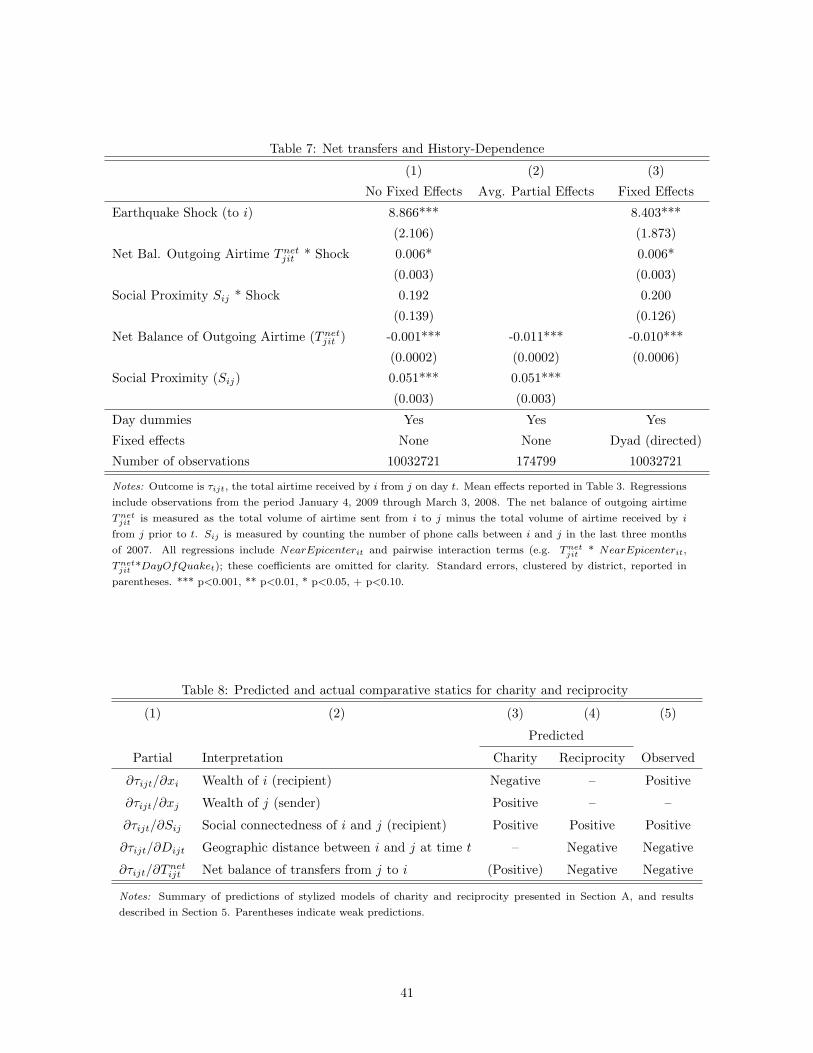
Table 7: Net transfers and History-Dependence

(1) (2) (3)

No Fixed Effects Avg. Partial Effects Fixed Effects

Earthquake Shock (to i) 8.866*** 8.403***

(2.106) (1.873)

Net Bal. Outgoing Airtime Tnetjit * Shock 0.006* 0.006*

(0.003) (0.003)

Social Proximity Sij * Shock 0.192 0.200

(0.139) (0.126)

Net Balance of Outgoing Airtime (Tnetjit ) -0.001*** -0.011*** -0.010***

(0.0002) (0.0002) (0.0006)

Social Proximity (Sij) 0.051*** 0.051***

(0.003) (0.003)

Day dummies Yes Yes Yes

Fixed effects None None Dyad (directed)

Number of observations 10032721 174799 10032721

Notes: Outcome is τijt, the total airtime received by i from j on day t. Mean effects reported in Table 3. Regressions

include observations from the period January 4, 2009 through March 3, 2008. The net balance of outgoing airtime

Tnetjit is measured as the total volume of airtime sent from i to j minus the total volume of airtime received by i

from j prior to t. Sij is measured by counting the number of phone calls between i and j in the last three months

of 2007. All regressions include NearEpicenterit and pairwise interaction terms (e.g. Tnetjit * NearEpicenterit,

Tnetjit *DayOfQuaket); these coefficients are omitted for clarity. Standard errors, clustered by district, reported in

parentheses. *** p<0.001, ** p<0.01, * p<0.05, + p<0.10.

Table 8: Predicted and actual comparative statics for charity and reciprocity

(1) (2) (3) (4) (5)

Predicted

Partial Interpretation Charity Reciprocity Observed

∂τijt/∂xi Wealth of i (recipient) Negative – Positive

∂τijt/∂xj Wealth of j (sender) Positive – –

∂τijt/∂Sij Social connectedness of i and j (recipient) Positive Positive Positive

∂τijt/∂Dijt Geographic distance between i and j at time t – Negative Negative

∂τijt/∂Tnetijt Net balance of transfers from j to i (Positive) Negative Negative

Notes: Summary of predictions of stylized models of charity and reciprocity presented in Section A, and results

described in Section 5. Parentheses indicate weak predictions.

41

Table 9: Placebo Tests - Region

(1) (2) (3) (4) (5)

3 month early 2 months early 1 month early Actual Quake 1 month late

placebo -2056.429 312.790 798.729 13326.179∗∗∗ -1089.114

(2471.31) (1662.70) (869.67) (1337.56) (1651.68)

placebo lag1 -4438.345 902.978 196.765 -992.363 -133.638

(3292.15) (1259.07) (1342.27) (1215.16) (3688.71)

placebo lag2 -1628.159 2961.500 80.133 1495.821 -7377.086

(1967.20) (2775.80) (2661.46) (2678.79) (5687.47)

placebo lag3 1370.931 1437.113 2430.937 789.919 -1949.726

(1115.80) (1711.70) (3958.41) (3092.60) (1931.41)

placebo lag4 -2393.805 -1599.899 -33.634 -207.856 -3785.758

(2354.55) (2108.57) (1691.97) (1407.14) (3793.98)

placebo lag5 1154.533 1153.144 611.661 -44.916 -3324.983

(1127.09) (1005.35) (1514.86) (2914.84) (2332.18)

placebo lag6 1482.134+ -1509.240 -324.826 -2662.037 -53.801

(748.31) (1069.94) (1044.35) (3156.40) (2037.16)

placebo lag7 1371.100+ 963.621 1542.388+ -401.769 1764.977

(709.54) (735.43) (807.87) (810.92) (2372.48)

Total calls 0.010 0.010 0.010 0.010 0.010

(0.01) (0.01) (0.01) (0.01) (0.01)

Outgoing transfers 0.878∗∗∗ 0.878∗∗∗ 0.878∗∗∗ 0.878∗∗∗ 0.878∗∗∗

(0.02) (0.02) (0.02) (0.02) (0.02)

Constant 2431.066∗∗∗ 2430.638∗∗∗ 2430.741∗∗∗ 2431.985∗∗∗ 2432.176∗∗∗

N 18990 18990 18990 18990 18990

Outcome: Value of incoming airtime sent to people in district (in RWF; US$1=500RWF). Heteroskedasticity-robust

SE’s in parentheses (clustered at district level).

42

Table 10: Lagged effects of the earthquake on transfers and calls received.

(1) (2) (3)

Transfers Received Calls Received Int’l Calls Received

Shock 13599.987∗∗∗ 14206.422∗∗∗ 141.634∗

(1051.04) (3762.18) (57.11)

shock lag1 -1200.544 4590.319∗∗∗ 124.644

(1129.42) (507.72) (77.40)

shock lag2 1444.242 1635.936 60.666

(2848.82) (1035.70) (50.72)

shock lag3 595.617 1293.153∗∗∗ 45.264

(3277.26) (299.40) (33.24)

shock lag4 -428.624 547.864∗ -30.650+

(1379.12) (206.22) (17.38)

shock lag5 -189.757 1066.467∗∗∗ -68.270∗

(3162.41) (228.90) (29.36)

shock lead1 567.236 224.344 32.700

(1886.17) (322.57) (25.67)

shock lead2 1198.341 215.258 38.347

(1119.03) (388.01) (44.66)

shock lead3 -2727.993 -77.107 -26.907

(1802.28) (207.44) (60.26)

shock lead4 -117.459 -489.221∗ -17.748

(2098.99) (194.31) (50.78)

shock lead5 6681.922 -83.052 17.834

(6234.18) (236.95) (58.40)

Outgoing transfers 0.884∗∗∗

(0.02)

Outgoing calls 0.969∗∗∗

(0.00)

Outgoing international calls 0.953∗∗∗

(0.02)

N 19200 19200 19200

Notes: Outcome is specified in column heading, aggregated at the district level. Regressions include

data from entire time window as described in Table 2 (October 2006 - July 2008). All specifications

include daily and district fixed effects. Heteroskedasticity-robust standard errors in parentheses

(clustered at district level).

43

Table 11: Effect of flood on transfers

(1) (2) (3) (4)

Pooled OLS OLS controls tower FE tower/Time FE

Flood shock 1455.411+ 772.401∗ 818.131∗ 849.166∗

(770.90) (290.32) (312.69) (344.89)

DaysOfF loodt 781.550∗∗∗ 361.117∗∗∗ 366.729∗∗∗

(166.88) (78.07) (72.11)

NearF loodRegionit 264.965 173.885∗∗

(919.89) (57.73)

Outgoing transfers 0.679∗∗∗ 0.640∗∗∗ 0.599∗∗∗

(0.03) (0.03) (0.03)

Total calls 0.088∗∗∗ 0.070∗∗∗ 0.084∗∗∗

(0.00) (0.01) (0.01)

Tower Fixed Effects No No Yes Yes

Date Fixed Effects No No No Yes

R2 0.000 0.785 0.804 0.811

N 170880 170880 170880 170880

“In flood region” defined as towers in the two districts affected by the flood. “Days of flood” are

9/12/07 - 9/18/07.

44

Appendix Tables

Appendix Table 1: Sensitivity of estimation to functional form assumptions

(1) (2) (3) (4)

Pooled OLS OLS w/Controls Region FE Region & Day FE

Earthquake Shock 2856.952∗∗∗ 2193.288∗∗∗ 2355.990∗∗∗ 2209.329∗∗∗

(416.57) (266.57) (176.02) (236.19)

DayOfQuake -717.340∗∗ -749.883∗∗∗ -679.739∗∗∗

(211.62) (98.79) (109.77)

NearEpicenterit -1342.708∗ -124.474∗∗∗

(546.53) (27.93)

Outgoing transfers 0.679∗∗∗ 0.640∗∗∗ 0.599∗∗∗

(0.03) (0.03) (0.03)

Total call volume 0.088∗∗∗ 0.070∗∗∗ 0.084∗∗∗

(0.00) (0.01) (0.01)

Tower Fixed Effects No No Yes Yes

Date Fixed Effects No No No Yes

R2 0.001 0.785 0.804 0.811

N 170880 170880 170880 170880

Notes: Outcome is the total amount transferred into a tower on a single day. NearEpicenter

defined as those towers within 20 miles of the earthquake epicenter. Columns 2-4 include controls

for overall network activity at the tower-day level. Column 3 includes tower-level fixed effects.

Column 4 includes daily fixed effects. Estimates made using data from October 1, 2006 through

July 1, 2008. Heteroskedasticity-robust SE’s in parentheses (clustered at district level). * p<0.05,

** p<0.01, *** p<0.001.

45

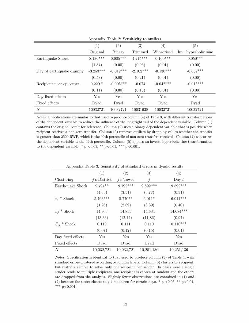
Appendix Table 2: Sensitivity to outliers

(1) (2) (3) (4) (5)

Original Binary Trimmed Winsorised Inv. hyperbolic sine

Earthquake Shock 8.136*** 0.005*** 4.275*** 0.100*** 0.050***

(1.34) (0.00) (0.96) (0.01) (0.00)

Day of earthquake dummy -3.253*** -0.012*** -2.102*** -0.130*** -0.052***

(0.53) (0.00) (0.21) (0.01) (0.00)

Recipient near epicenter 0.229 * -0.005*** -0.074 -0.042*** -0.015***

(0.11) (0.00) (0.13) (0.01) (0.00)

Day fixed effects Yes Yes Yes Yes Yes

Fixed effects Dyad Dyad Dyad Dyad Dyad

N 10032721 10032721 10031628 10032721 10032721

Notes: Specifications are similar to that used to produce column (4) of Table 3, with different transformations

of the dependent variable to reduce the influence of the long right tail of the dependent variable. Column (1)

contains the original result for reference. Column (2) uses a binary dependent variable that is positive when

recipient receives a non-zero transfer. Column (3) removes outliers by dropping values whether the transfer

is greater than 2500 RWF, which is the 99th percentile of non-zero transfers received. Column (4) winsorizes

the dependent variable at the 99th percentile. Column (5) applies an inverse hyperbolic sine transformation

to the dependent variable. * p <0.05, ** p<0.01, *** p<0.001.

Appendix Table 3: Sensitivity of standard errors in dyadic results

(1) (2) (3) (4)

Clustering j’s District j’s Tower j Day t

Earthquake Shock 9.794** 9.792*** 9.892*** 9.892***

(4.33) (3.51) (3.77) (0.31)

xi * Shock 5.763*** 5.770** 6.011* 6.011***

(1.26) (2.89) (3.39) (0.40)

xj * Shock 14.903 14.833 14.684 14.684***

(13.33) (12.12) (11.86) (0.97)

Sij * Shock 0.110 0.111 0.110 0.110***

(0.07) (0.12) (0.15) (0.01)

Day fixed effects Yes Yes Yes Yes

Fixed effects Dyad Dyad Dyad Dyad

N 10,032,721 10,032,721 10,251,136 10,251,136

Notes: Specification is identical to that used to produce column (3) of Table 4, with

standard errors clustered according to column labels. Column (5) clusters by recipient,

but restricts sample to allow only one recipient per sender. In cases were a single

sender sends to multiple recipients, one recipient is chosen at random and the others

are dropped from the analysis. Slightly fewer observations are contained in (1) and

(2) because the tower closest to j is unknown for certain days. * p <0.05, ** p<0.01,

*** p<0.001.

46

Appendix Table 4: Net transfers and wealth (Robustness to sender FE)

Earthquake Shock 9.727*

(4.36)

Recipient Wealth xi * Shock 5.702***

(1.31)

Sender Wealth (xj) * Shock 15.299

(13.93)

Social Proximity Sij * Shock 0.102

(0.07)

Recipient Wealth (xi) 0.847***

(0.17)

Social Proximity (Sij) 0.069***

(0.00)

Day dummies Yes

Fixed effects Sender j

Number of observations 10032721

Notes: Outcome is τijt, the total airtime received by i from j on day t. Re-

gressions include observations from the period January 4, 2008 through March

3, 2008. Wealth proxies xi and xj are computed using equations (6) and (7),

as described in the text. Sij is measured by counting the number of phone

calls between i and j in the last three months of 2007. All regressions include

NearEpicenterit and pairwise interaction terms (e.g. xi * NearEpicenterit,

xi*DayOfQuaket); these coefficients are omitted for clarity. Standard er-

rors, clustered by district, reported in parentheses. *** p<0.001, ** p<0.01, *

p<0.05, + p<0.10.

47

Appendix Table 5: Network Flow as Social Proximity

(1) (2) (3)

No Fixed Effects Avg. Partial Effects Fixed Effects

Shock (recipient) 8.935* 8.480+

(4.33) (4.16)

Recipient Wealth xi * Shock 6.791*** 6.806***

(0.75) (0.95)

Sender Wealth xj * Shock 16.501 15.766

(14.74) (13.66)

Network Flow Sij * Shock -0.918 -0.846

(0.62) (0.51)

Recipient Wealth (xi) 1.146*** 1.266***

(0.17) (0.10)

Sender Wealth (xj) 1.915*** 1.892***

(0.12) (0.14)

Network Flow (Sij) 0.048 0.054***

(0.03) (0.02)

Day dummies Yes Yes Yes

Fixed effects None None Dyad (directed)

Number of observations 10032721 10032721 10032721

Notes: Outcome is τijt, i.e. airtime received by i from j on day t. xi and xj are estimated using equations

(6) and (7), described in text. Sij measures the number of distinct paths between i and j, where a path

is defined by the call graph. All regressions include NearEpicenteri and pairwise interaction terms (e.g.

xi * NearEpicenteri, xi*DayOfQuaket), but results are omitted for clarity. Standard errors, clustered by

district, reported in parentheses. *** p<0.01, ** p<0.05, * p<0.1.

Appendix Table 6: Regression of Expenditures on Asset Ownership

Outcome log(Expenditures) Expenditures

βa (S.E.) βa (S.E.)

Radio 0.18 (0.02) 40090 (13007)

Television 1.14 (0.01) 2130434 (44048)

Bed 0.24 (0.04) 187061 (8266)

Table 0.13 (0.01) 57601 (9109)

Car/Truck 0.24 (0.01) 1695284 (57718)

Motorcycle 0.65 (0.04) 8229976 (197091)

Bicycle 0.22 (0.11) 138186 (20359)

HH Size 0.09 (0.02) 56168 (3198)

R2 0.62 0.75

N 6900 6900

Notes: Standard errors reported in parentheses.

48

Appendix Table 7: Summary statistics of phone use as computed from transaction logs

Average

Panel A: Domestic and International Calls

Activation date 1/12/08

Days of activity 770.3

Avg. call length 31.7

Calls per day 6.25

Net calls per day (out-in) 0.087

Int’l calls per day 0.084

Net int’l calls (out-in) -0.014

Panel B: Social Network Structure

Degree 734

In-degree 488.2

Out-degree 433

Daily degree 3.78

Net daily degree (out-in) 0.00027

Clustering 0.063

Betweenness 2.72

Panel C: Other Behaviors

Credit used per day 163.5

Max. recharge value 2756.3

Avg. districts per day 1.36

Avg. districts contacted 1.21

N 901

Notes: Mean values reported, weighted by sampling strata

to produce averages representative of entire phone popula-

tion.

49

Appendix Table 8: Regression of predicted expenditures on phone use

Coefficient (S. E.)

Num days phone was used 1078.9 (0.94)

Days2 0.511 (0.66)

Number of recharges -2178.4 (-0.72)

Recharges2 -5.063 (-1.75)

Total calls made 42.55 (0.08)

Calls made2 0.00446 (0.10)

Total calls received -1053.8 (-1.56)

Calls received2 0.0562 (0.82)

Duration (outgoing) 27.98∗∗∗ (3.46)

Duration (outgoing)2 -0.0000242∗∗ (-2.59)

Duration (incoming) 33.19∗∗ (2.74)

Duration (incoming)2 -0.0000354 (-1.29)

International calls made -7853.7 (-0.72)

International calls made2 43.95 (1.44)

International calls received -7191.3 (-0.70)

International calls received2 27.29 (1.06)

Degree (outgoing) -2607.8 (-0.29)

Degree (outgoing)2 14.01 (1.09)

Degree (incoming) -7925.6 (-0.71)

Degree (incoming)2 9.917 (0.85)

Int’l Degree 336694.7∗∗ (3.06)

Int’l degree2 -2.991 (-0.00)

Districts called -82424.9 (-0.78)

Districts called2 -1440.6 (-0.55)

Districts received -317282.5∗∗ (-3.06)

Districts received2 -86.57 (-0.07)

R2 0.392

N 901

Outcome is predicted expenditures Yid, in RWF. Standard errors in

parentheses. Regression includes district fixed effects. ∗ significant

at p < .05; ∗∗p < .01;∗∗∗p < .001.

50

Appen

dix

Tab

le9:

Net

tran

sfersan

dHistory-D

epen

den

ce,byTotal

balan

ce

PositiveNet

Individual

Balan

ceNegativeNet

Individual

Balan

ce

(1)

(2)

(3)

(4)

(5)

(6)

NoFixed

Effects

A.P.E.

Fixed

Effects

NoFixed

Effects

A.P.E.

Fixed

Effects

Shock

(recipient)

5.44

2∗∗

4.98

2∗∗

4.59

95.854

(1.55)

(1.67)

(14.98

)(14.06)

Net

Bal.OutgoingAirtimeT

net

jit

*Shock

0.01

0∗∗∗

0.00

00.01

0∗∗∗

0.01

80.00

00.017

(0.00)

(.)

(0.00)

(0.02)

(.)

(0.02)

Social

Proxim

itySij

*Shock

-0.057

∗∗0.00

0-0.042

∗∗0.18

0∗0.00

00.188∗

(0.02)

(.)

(0.01)

(0.07)

(.)

(0.07)

Net

Bal.OutgoingAirtimeT

net

jit

-0.001

-0.001

∗∗∗

-0.001

-0.002

∗∗∗

-0.029

∗∗∗

-0.026

∗∗∗

(0.00)

(0.00)

(0.00)

(0.00)

(0.00)

(0.00)

Social

Proxim

itySij

0.00

9∗∗∗

0.01

4∗∗∗

0.00

00.04

1∗∗∗

0.07

0∗∗

∗0.000

(0.00)

(0.00)

(.)

(0.01)

(0.01)

(.)

N43

4193

277

194

4341

932

5690

789

9760

55690789

Notes:

Outcomeis

τ ijt,th

etotalairtimereceived

byifrom

jondayt.

Mea

neff

ects

reported

inTable

3.Reg

ressionsincludeobservationsfrom

theperiodJanuary

4,2008

throughMarch3,2008.Thenet

balance

ofoutgoingairtimeT

net

jit

ismea

suredasth

etotalvolumeofairtimesentfrom

ito

jminusth

etotalvolumeofairtimereceived

byi

from

jpriorto

t.Sij

ismea

suredbyco

untingth

enumber

ofphoneca

llsbetweeniandjin

thelast

threemonth

sof2007.AllregressionsincludeNea

rEpicen

ter i

tandpairwise

interactionterm

s(e.g.T

net

jit

*Nea

rEpicen

ter i

t,T

net

jit

*DayOfQuake t);

theseco

efficien

tsare

omittedforclarity.Standard

errors,clustered

bydistrict,

reported

inparenth

eses.

***p<0.001,**p<0.01,*p<0.05,+

p<0.10.

51

Appendix Table 10: Full interaction specification

(1) (2) (3)No F.E. A.P.E. Fixed Effects

Shock (recipient) 7.261+ 6.965∗

(3.59) (3.38)Recipient Wealth xi * Shock 6.425∗∗∗ 6.176∗∗∗

(0.23) (0.33)Sender Wealth xj * Shock 15.238 14.662

(13.21) (12.14)Distance Dijt * Shock 0.070+ 0.069+

(0.04) (0.04)Net Bal. Outgoing Airtime Tnet

jit * Shock 0.006 0.006(0.00) (0.00)

Social Proximity Sij * Shock 0.112 0.127(0.10) (0.09)

Recipient Wealth xi 1.019∗∗∗ 0.935∗∗∗

(0.16) (0.11)Sender Wealth xj 1.553∗∗∗ 1.809∗∗∗

(0.11) (0.10)Distance Dijt -0.013∗∗∗ 0.004∗∗ -0.021∗∗∗

(0.00) (0.00) (0.00)Net Bal. Outgoing Airtime Tnet

jit -0.001∗∗∗ -0.011∗∗∗ -0.010∗∗∗

(0.00) (0.00) (0.00)Social Proximity Sij 0.040∗∗∗ 0.040∗∗∗

(0.00) (0.00)N 9703746.000 165264.000 9703746.000

Notes: Outcome is τijt, the total airtime received by i from j on day t. Regressions include

observations from the period January 4, 2008 through March 3, 2008. Wealth proxies xi and xj

are computed using equations (6) and (7), as described in the text. Dijt measures the distance

between i and j in kilometers on day t, using the locational inference algorithm described in

Section 4.1. The net balance of outgoing airtime Tnetjit is measured as the total volume of airtime

sent from i to j minus the total volume of airtime received by i from j prior to t. Sij is measured

by counting the number of phone calls between i and j in the last three months of 2007. All

regressions include NearEpicenterit and pairwise interaction terms (e.g. Tnetjit * NearEpicenterit,

Tnetjit *DayOfQuaket); these coefficients are omitted for clarity. Standard errors, clustered by

district, reported in parentheses. *** p<0.001, ** p<0.01, * p<0.05, + p<0.10.

52

Figures

Figure 1: Map of Rwanda showing the location of mobile phone towers (as of February 2008) and the locationof the Lake Kivu earthquake of 2008. Each black dot represents a cell tower, with the approximate areacovered by the tower demarcated by adjacent Voronoi cells. The epicenter of the earthquake is shown withred concentric circles.

53

Figure 2: Map of Rwanda showing a single individual’s inferred trajectory over a 6 month period. Althoughthe individual only makes a small number of phone calls, the locational inference algorithm is able to roughlyassign the user a continuous trajectory through time to places not restricted to the set of known locations ofcellular towers. This particular individual is observed to slowly migrate southeastward, with early locationscolored dark red and later locations colored yellow.

54

010

000

2000

030

000

4000

0

Date

Num

ber

of A

ctiv

e U

sers

/Day

Jan.06 Jul.06 Jan.07 Jul.07 Jan.08 Jun.08 Jan.09

Figure 3: Growth in active users of the Mobile Money transfer system, using data from January 2006 untilJanuary 2009. The service was first launched in late 2006, and uptake was low at the time of the LakeKivu earthquake, which is represented by the vertical line on February 3, 2008. Use of the service increasedrapidly beginning in mid-2008, when the operator began heavily advertising and promoting the product.Gaps indicate days with missing data (most notably from June 2008).

55

Distribution of distance between sender and recipient (km)

Distance in kilometers

Den

sity

0 50 100 150 200

0.00

0.02

0.04

0.06

0.08

0.10

(a) Transfer distances over 4 years

Distribution of distance between sender and recipient (km)

Distance in kilometers

Den

sity

0 50 100 150 200

0.00

0.02

0.04

0.06

0.08

0.10

2 months prior to earthquake2 days after earthquake

(b) Transfer distances just before/after quake

Figure 4: Distribution of distances over which transfers are sent to and from the earthquake region. AKolmogorov-Smirnow test rejects the equality of the two distributions in (b) with p ≤ 0.001.

56

Figure 5: Relationship between the geographic structure of an individual’s network and her propensity toreceive a transfer after the earthquake. Values on the y-axis correspond to the estimated coefficients fromon µ2 from regression (5), where Zi is the number of i’s contacts who live within R kilometers of i, with Rplotted on the x-axis.

57

Balance on account at end of day (RWF)

Den

sity

0 500 1000 1500 2000

0.00

00.

005

0.01

00.

015

Figure 6: Distribution of end-of-day account balances on February 1, 2008, the day before the Lake Kivuearthquake. Subscribers with balances in the top and bottom 0.5 percent of all users were removed toimprove the quality of the display (one user had a balance of 442500RWF).

58

Appendices

A Motives for Mobile Phone-Based Giving: Details

A.1 Charity

As discussed in the main text, the mobile phone-based giving that occurs in response to economic shocks is

statistically strong, though small in absolute terms. We defined a simple model of charity, by which we refer

to the broad class of motives where a giver gives because he receives direct utility from the act of giving or

from increasing the utility of another. The canonical example of this behavior is pure altruism, where one

person’s utility depends positively on another’s (Becker 1976, Andreoni & Miller 2002):

Uit = ui(xit − τjit) + γijuj(xj + τjit) (A.1)

As before, we denote by τjit a transfer sent from i to j at time t. Assuming ui(·) and uj(·) are increasing

and concave, with xi representing the income of individual i and γij denoting the level of altruism felt by i

toward j, it is easily shown that two predictions of such a model are

∂E[τji|xi]∂xi

≥ 0 and∂E[τji|xj ]

∂xj≤ 0 (A.2)

Giving is expected to increase in the income of the sender (as the marginal cost of giving decreases), and

decrease in the income of the recipient (as the marginal benefit of a gift decreases). Such predictions

are supported by observed patterns of altruism in a variety of contexts, including charitable giving in the

United States (Andreoni 2006) and the behavior of “rescuers” in Nazi-occupied Europe during World War

II (Hoffman 2010).20

Through similar logic, we expect that in cases of directed altruism, where γij varies across dyads, transfers

decrease with the social distance between i and j. However, ceteris paribus and conditional on an appropriate

measure of social distance, there should be no relationship between transfers and geographic distance. Finally,

in the simple model specified by (8), we expect current transfers between i and j to be “memory-less”

(Fafchamps & Lund 2003), i.e. current transfers should not depend on the past history of i-j transfers –

so as long as we can control for other time-invariant aspects of the i-j relationship. To the extent that an

20While the comparative statics in (A.2) are most transparent in the model of linear altruism specified by equation (8), similarpredictions obtain from several related models of charitable behavior, and we make no pretense to be able to distinguish betweenthem. Thus, models of inequity and inequality aversion (where i seeks to minimize |xi − xj |), social welfare models (where imaximizes min{x1, ..., xn}), and warm glow giving (where v(xj + τji) in (8) is replaced with τji) all yield similar predictions(cf. Fehr & Schmidt 1999, Bolton & Ockenfels 2000, Charness & Rabin 2002, Andreoni 1990, List & Lucking-Reiley 2002).

59

association does exist between past transfers and current transfers, we would expect it to be positive, as

past transfers may reveal information about how much i cares about j, above and beyond the undirected

measures of relationship strength that we employ. These predictions are summarized in column (3) of Table

8.

A.2 Conditional reciprocity

By conditional reciprocity, we refer to motives that are embedded in long-term relationships of bilateral

exchange. We focus here on instrumental reciprocity, where mutual exchange is motivated by the expectation

of future reciprocation (cf. Coate & Ravallion 1993, Karlan et al. 2009), as this model most transparently

leads to empirical predictions that can be tested with the data at our disposal. Other models of reciprocity,

and most notably the intrinsic, preference-based reciprocity modeled by Rabin (1993) and Falk & Fischbacher

(2006), produce similar predictions. However, since our intent is not to differentiate between these different

types of conditional reciprocity, we present a simple model of dynamic limited commitment that captures

many of the central tenets of the wider literature.21

The basic idea is easily illustrated by a model of risk sharing under dynamic limited commitment (Ligon

et al. 2002, Foster & Rosenzweig 2001). Following Foster & Rosenzweig (2001), we assume i has stationary,

single-period utility specified by (8), but allow for the possibility that i expects to benefit from future

interaction with j:

Uit = ui(xit − τjit) + γijuj(xjt + τjit) + E

∞∑s=t+1

δs−t[ui(xis − τjis) + γijuj(xjs + τjis)] (A.3)

The first part of this equation is identical to the altruistic model (8), while the second term captures the

discounted expected utility of the relationship.

This formulation produces two key insights relevant to the current analysis. First, when contracts are

not fully enforceable ex-post, transfers received in the current period will depend on past transfers given.

Models using conditional reciprocity norms generate the same prediction. For the LC model, this property

is formally derived in Appendix A.3, however the intuition is straightforward: In the stationary model of

(8), i and j will transfer the necessary τjit to equate the ratio of their ex post marginal utilities to γ (or 1/γ

if xi < xj). If γ is sufficiently small, i and j operate in autarky. By contrast, in the dynamic model specified

by (9), i and j also derive utility from expected future interactions and transfers, and so may adjust the

ratio of marginal utilities at time t to maintain the relationship and avoid reversion to a series of static Nash

21For recent experimental work that differentiates between different types of reciprocity, see Leider et al. (2009), Ligon &Schechter (2011), and Cabral et al. (2011). Kinnan (2014) provides a test between different barriers to informal insurance inrural villages.

60

equilibria. Intuitively, when i suffers a shock in period t, the marginal utility of τijt will be quite high and

so he will be willing to sacrifice a greater share of his continuation utility in exchange for a larger transfer at

t. As a result, we expect transfers from i to j sent in response to a shock to be decreasing in the net balance

of transfers previously made from i to j (denoted by Tnetjit ):

∂E[τjit|Tnetjit ]

∂Tnetjit

≤ 0 where Tnetjit =

t−1∑s=0

τjis − τijs (A.4)

As robustness checks, we further expect that τjit will decrease in the gross volume of prior transfers from i

to j (denoted by Tjit) and increase in gross prior transfers from j to i (denoted by Tijt):

∂E[τjit|Tjit]∂Tjit

≤ 0 and∂E[τjit|Tijt]

∂Tijt≥ 0 where Tjit =

t−1∑s=0

τjis

This model of dynamic limited commitment has been shown to account for empirical evidence better than

a stationary model with no history-dependence (Ligon et al. 2002, Genicot & Ray 2003, Fafchamps &

Lund 2003).

A second point of contrast between the model of charity (8) and conditional reciprocity (9) pertains to

the marginal effect of geographic distance on transfers. Under the second formulation, and as discussed by

Ligon (1998) and De Vreyer et al. (2010), transfers are expected to decrease as, ceteris paribus, the cost

of monitoring and enforcement increases. Assuming that such monitoring and enforcement costs increase

monotonically with geographic distance Dij , we expect that:22

∂E[τij |dij , Sij ]

∂dij≤ 0 (A.5)

i.e., conditional on the strength of the social connection between i and j, the further away j resides from

i, the less likely is j to help i following an idiosyncratic shock. Of course, distance is likely correlated with

other factors that influence the decision to give, but which are not related to monitoring and enforcement

per se.23 Thus, when we operationalize (A.5) in a regression setting, we always condition our empirical

results on Sij , an undirected measure of the strength of the relationship between i and j, and a dyad fixed

effect πij , so that we estimate the partial effect of geographic distance holding constant other unobservable

characteristics of the dyad.

The predictions of model (9) are summarized in column (4) of Table 8. Unlike the model of charity, the

22This could be the case if, for instance, j must visit i to verify damage to i’s property, and the cost of travel increases withdistance.

23For instance, transaction costs, which often rise with distance, have received recent attention by Jack & Suri (2012).However, since the cost of remitting over the Rwandan mobile network is free at all distances, transaction costs are unlikely todrive empirical estimates of (A.5).

61

model of reciprocity does not make strong predictions regarding the relative wealth of i and j. We might

expect transfers to go to wealthier individuals if strategic agents seek to ingratiate themselves for future

reciprocation. Such an interpretation is supported by recent work by Schechter & Yuskavage (2011), who find

that transfers are likely to flow from more to less wealthy households in unreciprocated relationships, while

reciprocated relationships are more likely between wealthier households. Alternatively, we could observe flows

from the rich to the poor if the poor reciprocate in ways other than airtime (Fafchamps 1999, Platteau 1995).

In Section 5, we will estimate the partials of equations (4) and (5) to adjudicate between the conflicting

predictions of models (8) and (9). First, however, we describe the data used in the analysis, as well as our

methods for measuring each component of our empirical specifications.

A.3 History-Dependence in Reciprocity

We derive the history-dependence of current period transfers in the model of dynamic limited commitment

presented in Section A.2. The exposition is based on Ligon et al. (2002) and Foster & Rosenzweig (2001),

but makes explicit the extension to the case where single-period utility includes a component of altruism.

Other models of reciprocity, and in particular the preference-based reciprocity of Rabin (1993) and Falk

& Fischbacher (2006), are predicated on fundamentally different “reciprocal” motives, but yield similar

empirical predictions. We employ the enforced/instrumental model because the comparative statics that

result are most directly testable with the data at our disposal, but do not mean to imply that the behavior

we observe is necessarily motivated by this particular type of reciprocity vs. a different type of reciprocity.

We rely on a model with two agents i and j with von Neumann-Morgenstern utility where i’s single

period utility in increasing in j’s single period utility according to (8), and vice versa. In static equilibrium,

non-zero transfers occur when i’s marginal utility of consumption is less than the γ-weighted utility of j,

i.e., when

u′i(xit) < γu′j(xjt) (A.6)

or when the converse applies to j.24 Call this static transfer, which depends on the state s of the world, τNjit,

where the superscript N denotes that this is the static Nash equilibrium. It is easily seen that whenever

(A.6) holds, i will transfer a non-zero τNjit that satisfies

u′i(xit − τNjit)

u′j(xjt + τNjit)= γ (A.7)

When the converse of (A.6) applies (i.e. u′j(xjt ≤ γu′i(xit)), the transfer will be negative, and in all other

24For simplicity we assume that i and j are similarly altruistic, i.e., γij = γji = γ.

62

cases the transfer will be zero.

In the repeated-game setting, agents are infinitely lived but are unable to save across periods. Given

uncertainty as to the state of the world that will be realized in the future, both i and j can potentially be

made better off through (possibly negative) state-contingent transfers τjit. The current-period utility of i is

then the sum of single period utility plus the expected discounted utility of future interaction with j, where

δ is the discount factor:

UTit = ui(xit − τjit)︸ ︷︷ ︸

own consumption

+ γuj(xjt + τjit)︸ ︷︷ ︸altruistic benefit︸ ︷︷ ︸

single period utility

+E

∞∑s=t+1

δs−t[ui(xis − τjis) + γuj(xjs + τjis)]︸ ︷︷ ︸continuation value of relationship

(A.8)

Though i and j may agree ex ante to a set of state-contingent transfers, imperfect ability to enforce

contracts implies limited commitment ex post. After the state of the world is realized, either agent can

renege at any time, in which case both i and j will revert to the static Nash equilibrium where τjit = τNjit as

given by (A.7). Then, i’s utility is simply

UAit = ui(xit − τNjit) + γuj(xjt + τNjit) + E

∞∑s=t+1

δs−t[ui(xis − τNjis) + γuj(xjs + τNjis)] (A.9)

The set of sustainable contracts are then defined by the implementability constraints that require utility

for both agents to be (weakly) greater than under the static Nash equilibrium, i.e., UTit ≥ UA

it and UTjt ≥ UA

jt .

These constraints specify a superset of sustainable contracts, a subset of which are efficient.

In the repeated game, the transition matrix Π specifies the probabilities psr = Pr(Xt+1 = r|Xt = s) of

transitioning from state s at time t to state r at time t+ 1, where S is the state space of the Markov chain.

The set of constrained-efficient contracts along the Pareto frontier can then be characterized as

Ujs(Uis) = maxτjit

{uj(xjt + τjit) + γui(xit − τjit) + δ

∑r∈S

psrUjr(Uir)

}(A.10)

Where Uis denotes the expected discounted utility of i given state s at time t, which j is required to satisfy.

63

The following conditions must be met for (A.10) to be optimal:

λ :[ui(xit − τjit)− ui(xit − τNjit)

]+γ[uj(xjt + τjit)− uj(xjt + τNjit)

]+δ∑r∈S

psrUir ≥ 0

δpsrϕr : Uir ≥ 0

δpsrµr : Ujr(Uir) ≥ 0

ψi : xit − τjit ≥ 0

ψj : xjt + τjit ≥ 0

With ui(·) and uj(·) concave, Ui(·) and Uj(·) are also concave, implying the following first order conditions

(??-??) and envelope condition (A.11):

u′j(xjt + τjit) + γu′i(xit − τjit)

ui(xit − τjit + γu′j(xjt + τjit)=λ+

ψi − ψj

u′(xit − τjit) + γv′(xjt + τjit)(A.11)

−V ′r (Ur) =

λ+ ϕr1 + µr

(A.12)

λ =u′j(xjt + τjit) + γu′i(xit − τjit)

u′i(xit − τjit) + γu′j(xjt + τjit)

=− V ′s (Us) (A.13)

The optimal contract is thus characterized by the slope of the Pareto frontier, λ, which determines the extent

to which i can transfer current-period utility to j. For each state, there exists a set of implementable points

on the Pareto frontier between λmins and λmax

s .

The history dependence arises as follows. When i and j first enter a relationship at t = 0, they agree

upon a contract that specifies a fixed ratio of marginal utilities λ0, which is a point on the Pareto frontier.

Once the state of nature becomes known at t = 1, i and j will attempt the τ∗jit that maintains the ratio of

marginal utilities at λ0. For simplicity, assume that at t = 1, j suffers a negative shock such that xi1 > xj1,

though the same logic applies when xi1 ≤ xj1. Then, in order to maintain λ0, the agents will attempt

τ∗jit > 0. However, if τ∗jit > 0 is large enough to make the implementability constraint on i bind, then i and

j will implement τjit < τ∗jit in order to avoid the static Nash equilibruim τNjit and preserve the continuation

value of the relationship. The implemented τjit will be just sufficient to relax the constraint on i, and a new

constrained-efficient ratio of single-period marginal utilities λt will be determined according to (??).

If the implementability constraints never bind (intuitively, this occurs when income covariance between

i and j is high), then agents will continue to equate marginal utilities at λ0 and there will effectively be no

history dependence in τjit. However, when a constraint binds, the dynamic model allows the worse-off agent

64

to sacrifice future consumption (by accepting a less favorable ratio of utility λ) in exchange for a transfer in

the current period. This recalibration of λ affects all subsequent τjit.

65

B Robustness

B.1 Functional form assumptions

We briefly show that our central results are not sensitive to the precise econometric specification, or to the

choice of time window (which in most regressions is restricted to the period starting one month before the

earthquake and ending one month after the earthquake). Appendix Table 1 presents estimates of the average

treatment effect of model (1) using the full dataset from October 2006 until July 2009 under a variety of

econometric specifications. Column (1) gives the standard OLS results with no control variables Xrt, time

fixed effects θt, or tower fixed effects πr. Column (2) includes time-varying controls to account for regional

variation in mobile phone use, column (3) adds regional fixed effects, and column (4) adds daily dummy

variables. Across all specifications, the estimated effect of the shock remains strong and significant, and of

a magnitude similar to that presented in Table 3.

B.2 Sensitivity to Outliers

To address the possibility that our effects are driven in part by outliers or a dependent variable with a

long right tail, we run a series of robustness checks in Appendix Table 2. Column (1) contains the original

results from column (4) of Table 3 for reference. Column (2) transforms the dependent variable (τijt) into

a binary indicator that is one when τijt > 0 and zero otherwise. Column (3) trims outliers by dropping

observations with τijt > 2500RWF, where 2500RWF is the 99th percentile of non-zero transfers received.

Column (4) winsorizes the dependent variable at the 99th percentile following Tukey (1962) by replacing all

values greater than the 99th percentile (2500RWF) with values at the 99th percentile. Column (5) applies the

inverse hyperbolic sine transformation to reduce the influence of extreme observations of dependent variables

(Burbidge et al. 1988). In all cases, the primary coefficient of interest is still positive and statistically

significant.

B.3 Robustness of Dyadic Regressions

In the body of the paper, we use dyadic regressions to measure which types of individuals i and j are most

likely to receive and send transfers in response to the earthquake. Tables 4 and 7 employ dyad-specific fixed

effects to control for unobserved, time-invariant characteristics of the dyad. Thus, the coefficient on the

interaction between xi and Shockit in Table 4 indicates the extent to which wealthier individuals i are more

likely to receive a transfer after the earthquake, in relation to the normal activity observed between i and j.

This specification, formalized in equation (5), reduces biases resulting from unobserved characteristics of i,

66

j, and the dyad i-j that could be correlated with the error term ϵijt. For instance, if i sends a large transfer

to j on each day of the year (for reasons unrelated to economic shocks), the dyadic fixed effects will ensure

that a large transfer sent from j to i on the day of the earthquake is not mis-attributed to the effect of the

earthquake.

As a robustness check, we demonstrate that our key results hold if the regressions are estimated with a

more parsimonious model that replaces the dyad-specific fixed effects (for each pair i-j) with sender-specific

fixed effects (for each sender j). This model is slightly less restrictive, and more directly corresponds to the

intuition that motivates the dyadic results, i.e., that we wish to identify the types of people i (where type

is proxied by xi) are chosen by j to receive a transfer, conditional on j’s average behavior. Formally, we

estimate the following model:

τijt = δ0 + δ1Shockit + δ2xi + δ3xiShockit + δ4xjShockit +

δ5NearEpicenterit + δ6xiNearEpicenterit + δ7xjNearEpicenterit +

δ8xiDayOfShockt + δ9xjDayOfShockt + θt + πj + εijt (B.1)

While the full specification of (B.1) is somewhat dense, all of the coefficients of interest are contained on

the first line, represented by δ1-δ4. The remaining δ5-δ9 are sub-interaction terms that are included for

consistency but which have limited real-world significance. To interpret, δ1 indicates whether individuals

affected by the earthquake (for whom NearEpicenterit = 1 and DayOfShockt = 1) are more likely to

receive a transfers; δ2 indicates whether wealthier individuals are more likely to receive more under normal

circumstances; δ3 indicates whether wealthier individuals receive more because of the earthquake; and δ4

indicates whether wealthier individuals send more to friends affected by the earthquake. All estimates are

conditional on the average amount sent by j.

Results from estimating model (B.1) are presented in Appendix Table 4. Only very minor differences

exist between these results and those presented in Table 4. Transfers sent in response to the earthquake

increase significantly in the wealth of the recipient, but are not significantly related to the wealth of the

sender. In other words, holding the identity of the sender fixed, it is the wealthier individuals – not the

poorer individuals predicted by models of charity – who are most likely to receive a transfer.

B.4 Measuring social proximity

In the regression results presented in the body, we control for the strength of the relationship between i and

j with Sij , which is simply the total number of calls made between i and j (in either direction) in the year

67

prior to the window of time used in the regressions. We choose this metric as a simple and easy to compute

statistic that is likely to be correlated with the overall social proximity of i and j. However, several other

such measures of Sij are also reasonable. In particular, Karlan et al. (2009) and Leider et al. (2009) suggest

a related metric, network flow, which captures the number of distinct paths between i and j through third

parties k. The intuition is that each common friend k increases the shared social collateral between i and j.

In Appendix Table 5, we show that our results are not sensitive to the specific measure of social proximity

used. The estimates in Appendix Table 5, which utilize network flow to measure Sij , are quite similar to the

estimates in Table 4, which measure Sij as the total number of prior phone calls. Controlling for network

flow in the other regressions similarly has no effect.

B.5 Standard errors

As discussed in Section 3, for standard error estimates to be consistent in the dyadic regressions, they should

ideally be cross-clustered by sender i and recipient j. This is because transfers involving the same individual

are likely to be correlated with each other – e.g., if j transfer airtime to i, he is ceteris paribus less able to

transfer airtime to others. In the results presented so far we have clustered standard errors by the district

in which the recipient resides.

As a robustness check, Appendix Table 3 compares alternative methods of obtaining standard errors

using different levels of clustering: no clustering (column 1), by recipient (column 2), by sender (column 3),

and by date (column 4). Standard errors are largest when we cluster by recipient, but in all specifications

the coefficients of interest remain significant.

68