0

Political Party Connections and the Diffusion of Technology:

Evidence from Britain’s first transport Revolution

Dan Bogart

Department of Economics, UC Irvine

3151 Social Science Plaza Irvine CA 92697-5100

dbogart@uci.edu1

This Draft: July. 2014

Abstract

Britain’s first transport revolution provides a revealing and important context to study the role of

political party connections in the diffusion of technologies. This paper focuses on river

navigation projects authorized by acts of parliament and the role of connections to the majority

political party in the House of Commons. It exploits the frequent turnover in majority parties

between the Whigs and Tories to construct exogenous changes in majority party representation

near all towns in Britain. The empirical analysis shows that the extension of navigation to a town

was less likely when the opponents of projects had more representation by the majority party in

the Commons. It also shows that electoral outcomes for the majority party were better in

opposition areas when river navigation bills were rejected in the Commons. The results provide

the first rigorous evidence that political party connections among vested interests can block the

diffusion of technologies.

JEL Code: N43, P16, D72

Keywords: Technology Diffusion, Lobbying, Transport, Political Parties, Glorious Revolution

1 I would like to thank Robert Oandasan, Larry Bush, Thomas Wheeler, Amanda Compton, and Alina Shiotsu for

providing valuable research assistance. I also thank Leigh Shaw Taylor for sharing population data and Stergios

Skepardis, John Wallis, Steve Nafziger, David Chambers, Latika Chaudhary, Gary Cox, and Gary Richardson for

helpful comments on earlier drafts. Also I thank participants at the Caltech Early modern group 2012, the 2012

ISNIE meetings, the Western Economic Association meetings, and seminar participants at UC Irvine, Lund

University, Oxford University, University of Edinburgh, Cambridge University, University of Arizona, UCLA,

USC, University of Maryland, Yale, and the Institute for Historical Research for their comments. Lastly I thank the

UC Irvine Council on Research, Computing, and Libraries for grant support. All errors are my own.

1

Good Roads, canals, and navigable rivers, by diminishing the expense of carriage, put the remote

parts of the country more nearly upon a level with those in the neighborhood of the town. They

are upon that account the greatest of all improvements….It is not more than fifty years ago that

some of the counties in the neighborhood of London, petitioned the parliament against the

extension of the turnpike roads into the remoter counties. Those remoter counties, they

pretended, from the cheapness of labour, would be able to sell their grass and corn cheaper in the

London market than themselves, and would thereby reduce their rents, and ruin their cultivation.

Adam Smith, the Wealth of Nations, Chapter XI, Of the Rent of Land (1976 p. 164).

I. Introduction

Adam Smith is well known for his observations on the gains from trade, but he also shrewdly

observed that vested invested interests sometimes block the adoption of technologies that benefit

most of society. In the passage above, Smith notes that landowners close to major markets

lobbied against the extension of turnpike roads and river navigation during the early 1700s. The

legal and political nature of these technologies made them especially prone to lobbying efforts.

River navigation projects, for example, had to be authorized by acts of parliament because they

involved the creation of corporate powers, like the compulsory purchase of land and the

introduction of tolls on waterways previously in the public domain. The landowners and towns

who opposed river projects exploited the political process by petitioning the House of Commons

to reject authorizing bills. Vested interests were successful up to a point. The diffusion of river

navigation projects was slow from 1690 to 1740, in part because many bills proposing projects

failed in the Commons several times before approval.

In this paper, I offer a new interpretation for the diffusion of river navigation acts. Like

Adam Smith my argument points to vested interests, but unlike Smith I emphasize the political

party connections of vested interests opposing river projects. The Whigs and Tories were the two

dominant parties in early eighteenth century Britain. They traded places as the majority party

2

seven times between 1690 and 1721, after which the Whigs remained as the majority party for

over 40 years. The Whigs and Tories influenced national policies dealing with government

finance and international trade, but they also influenced local economic policies. As I show

below river acts were less likely to be adopted in towns where the likely opponents of these acts

had stronger representation by the majority party in the Commons. Specifically, I show that

opposition to river bills was strongest in areas ‘downstream’ from the project and within 25

miles. I then document that having more majority party Members of Parliament (MPs) in

downstream areas within 25 miles meant that a town was less likely to get a river navigation act.

One potential concern is that opposition groups could campaign to get majority party

MPs elected. In the baseline fixed effects model, identification comes from variation in the

number of majority party MPs near a town and across parliaments. While time-invariant

unobservable characteristics are controlled for, there is still a possibility that time-varying

unobservable factors could influence the capability for opposition groups to get majority party

MPs elected and to lobby for the rejection of bills. To address this problem I use cases where

there was a new majority party in the Commons and the same MP was elected and remained

affiliated with their previous party as an exogenous source of variation for changes in majority

party MPs near the town. The results are similar to the baseline model and suggest that the

political connections of opponents are not endogenous.

The same conclusion does not apply to the political connections of supporters. As I show

below, support for river navigation acts was concentrated in towns where navigation was being

extended or it was in upstream areas within 25 to 40 miles. Drawing on these patterns I use

proximate and upstream majority party MPs as my indicator for the political connections of

likely supporters. In the baseline model, there is evidence that having more upstream majority

3

party MPs meant that a town was more likely to get a river navigation act. However, these

effects are not present when exogenous sources of variation in majority party MPs are used. Thus

the political connection of supporters is likely to be endogenous.

Other political factors are incorporated in the analysis and complement the main findings.

For example, greater political competition downstream from a town lowers its likelihood of

getting a river navigation act. The effects of political competition also differ depending on

whether the Whigs or Tories were in the majority. Under the Whigs political competition had a

stronger negative effect on adoption. Interestingly, having more incumbent MPs upstream or

downstream has no significant effect.

In the last section of the paper I examine the behavioral mechanisms underlying the

results. One theory is that the promoters of river bills were informed about the political party

connections of opponents to river bills and understood the implications for their bill’s success in

parliament. Another theory is that promoters were misinformed about connections or did not

understand their implications. I find evidence in favor of the latter theory using data on the

introduction of river bills and their success in parliament. Regression analysis shows that

majority party strength downstream and within 25 miles has no significant effect on the

introduction of bills in a town but it significantly increases the probability of a town’s bill

succeeding in Parliament. I also provide evidence that the majority party in the Commons

targeted rejections to connected opposition groups in order to maintain their majority status. This

finding is consistent with the political science literature which argues that political parties often

target policies to core supporters in order to maximize their electoral success (Cox and

McCubbins 1986, Lindbeck and Weibull 1987, Dixit and Londregan 1996).

4

My results contribute to several literatures. The first looks at the effects of political

connections on firm-level outcomes. In the majority of these studies, connections are measured

through campaign contributions or the personal relationships between politicians and either firm

managers, corporate board members, or employees. These studies generally find evidence for a

link between political connections and regulatory policies favorable to the firm (Faccio et. al.

2006) or between connections and the market value of firms (Faccio 2006, Blanes i Vidal et. al.

2012, Cingano and Pinotti 2013). However, relatively few papers rigorously study the effects of

connections to the majority political party. An exception is Jayachandran (2006) who documents

the effects of an exogenous change in majority party connections following Senator Jim Jeffords

exit from the Republican Party that tipped control of the U.S. Senate to the Democrats. Another

is Ferguson and Voth (2008) who show that connections to the National Socialist German

Workers’ Party increased the market value of German firms in the 1930s. This paper adds to this

literature by demonstrating the effects of political party connections in Britain during a formative

period in its history. This historical setting is especially revealing because there was frequent

turnover in the majority party. In most modern contexts, the majority party changes infrequently,

making the identification of political party connections challenging, if not impossible. This paper

uses the frequent turnover to measure exogenous changes in majority party connections in a

novel way.

This paper also relates to the broader literature studying political parties and their

influence on economic outcomes. Most of the targeting literature has emphasized spending or

national policies. For example, there is evidence that government spending patterns differ when a

district or region is strongly represented by the majority party (Lee 2003, Levitt and Synder

2005, Knight 2008, Curto Grao et. al. 2012, Albouy 2013, Burgess et. al. 2013). In the British

5

historical context, Stasavage (2005, 2007) provides evidence that whether the Whigs or Tories

were the majority party influenced government bond yields. This paper is novel because it relates

political party connections to regulatory policies affecting technology and the granting of

corporate powers. The only similar type of analysis in the literature is by Besley, Persson, and

Sturm (2010) who provide evidence for a link between political party competition and anti-

growth policies across US states.

Another related literature concerns the link between vested interests, institutions, and the

diffusion of technologies. This literature is motivated by the stylized fact that poor countries are

slower to adopt best practice technologies and hence have lower productivity (Parente and

Prescot 2000, Bellettini, Berti Ceroni, and Prarolo 2014). Comin and Hobijn (2009)

demonstrates that in countries with weak institutions, the existence of a close predecessor

technology slows the diffusion of new technologies. Relatedly a number of historical works

argue that resistance to technologies and corporations by vested interests is one of the main

reasons economies grew slowly in the past, including Britain in the early eighteenth century

(Mokyr 1990, Mokyr and Nye 2007, North, Wallis, and Weingast 2009). In these works, river

navigation acts are not the typical example of blocked technologies; nevertheless they were

significant in their time. As noted by Adam Smith, investments in the expansion of markets were

among the most important innovations in the pre-industrial world. Moreover, powers of eminent

domain and user-fee systems based on tolls are common in the modern world, but they were

untested legal technologies in the early 1700s. In fact most countries did not develop

infrastructure financing systems until the railway era of the nineteenth century. In short, the

finding that political party connections slowed the diffusion of river navigation acts in the early

1700s meant that politics influenced the pace of Britain’s economic growth.

6

II. Background on Political Parties and Government Policy in Britain

The Glorious Revolution of 1688 marked a significant turning point in the political history of

Britain. Over the next two decades the House of Commons and Lords solidified a key role for

Parliament in governing the country. The House of Commons, in particular, developed the fiscal

and implicit constitutional power to check the authority of the Monarchy. Britain was fairly

unique in this aspect because elsewhere in Europe representative institutions became dormant

(North and Weingast 1989, Bosker, Buringh, and Luiten van Zanden, 2012).

Politics in the aftermath of the Glorious Revolution were strongly influenced by competition

between Britain’s first political parties: the Whigs and Tories. They differed in their policy

positions with the Tories favoring privileges for the Church of England, lower taxes, and a small

government debt. The Whigs generally favored religious toleration and an aggressive foreign

policy based on a well-funded army. The two parties also differed in their supporters. The Tories

were generally supported by small to medium landowners known as country gentleman. The

Whigs drew more support from merchants and large landowners.

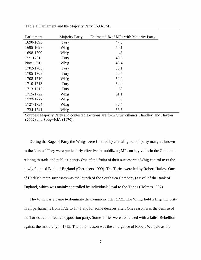
The Whigs and Tories vigorously competed in elections between 1690 and 1721, a period

known as the ‘Rage of Party.’ There were 11 elections and the majority party in the Commons

changed seven times (see table 1). Cruickshanks, Handley, and Hayton’s (2002) estimates on the

size of majority parties suggest they could be quite large as in the 1710 to 1713 Parliament with

more than 60 percent of MPs being linked to the Tories. They could also be relatively small as in

1705 to 1708 when the Tories held a narrow majority close to 50 percent.

7

Table 1: Parliament and the Majority Party 1690-1741

Parliament Majority Party Estimated % of MPs with Majority Party

1690-1695 Tory 47.5

1695-1698 Whig 50.1

1698-1700 Whig 48

Jan. 1701 Tory 48.5

Nov. 1701 Whig 48.4

1702-1705 Tory 58.1

1705-1708 Tory 50.7

1708-1710 Whig 52.2

1710-1713 Tory 64.4

1713-1715 Tory 69

1715-1722 Whig 61.1

1722-1727 Whig 68

1727-1734 Whig 76.4

1734-1741 Whig 68.6

Sources: Majority Party and contested elections are from Cruickshanks, Handley, and Hayton (2002) and Sedgwick's (1970).

During the Rage of Party the Whigs were first led by a small group of party mangers known

as the ‘Junto.’ They were particularly effective in mobilizing MPs on key votes in the Commons

relating to trade and public finance. One of the fruits of their success was Whig control over the

newly founded Bank of England (Carruthers 1999). The Tories were led by Robert Harley. One

of Harley’s main successes was the launch of the South Sea Company (a rival of the Bank of

England) which was mainly controlled by individuals loyal to the Tories (Holmes 1987).

The Whig party came to dominate the Commons after 1721. The Whigs held a large majority

in all parliaments from 1722 to 1741 and for some decades after. One reason was the demise of

the Tories as an effective opposition party. Some Tories were associated with a failed Rebellion

against the monarchy in 1715. The other reason was the emergence of Robert Walpole as the

8

leader of the Whigs. Serving as the first Prime Minister from 1721 to 1742, Walpole was

especially effective in using government favors to secure a working majority in the Commons.

The organizational capacity and relevance of Britain’s early political parties has been debated

by historians. In an influential work, Namier (1957) and Walcott (1956) argued that political

parties were largely irrelevant for policy-making. Research followed which showed that the

Whigs and Tories were more capable than Namier and Walcott suggested. The current consensus

is that from 1695 to 1740 Britain’s early parties were not as effective as modern parties, but they

were still capable of organizing and carrying out party strategies. Geoffrey Holmes, a leading

historian of politics from 1702 to 1714, summarizes this view: “neither possessed a party

machine in any strict sense, nor the regular income needed to maintain one; neither employed a

system of official whips whose authority was generally recognized. Yet party organization of a

kind was undoubtedly achieved in the years from 1702 to 1714, more susceptible to failure,

inevitably, than its formalized modern equivalent, but also capable at times of surprising

effectiveness (1987 p. 287).” 2

The economic history literature provides some supporting evidence that political parties

affected government policies, especially when they held a majority in the Commons. Stasavage

(2003, 2007) provides evidence that British government bond yields were lower when the Whigs

had a larger majority and higher when the Tories were in the majority. Stasavage argues that

government bondholders were a key part of the Whig coalition and that the Junto and Walpole

recognized that to stay in power the Whigs needed to protect bondholder rights. Dudley (2013)

argues that the Whigs were more favorable to the manufacturing sector and worked to assist this

2 For the historical literature on Britain’s parties see Speck (1970), Hill (1976), Horowitz (1977), Harris (1993).

9

sector when they had a majority in the Commons. Pincus (2009) and Pincus and Robinson

(2013) also see the Whigs as having an ideology more favorable to manufacturing.

Each of these studies is convincing to a degree. The only quantitative studies are by

Stasavage (2003, 2007) and there the evidence comes from time-series variation in government

bond yields and the identity or size of the majority party in the Commons. More compelling

identification strategies are needed as in the contemporary literature on political connections and

parties. Moreover, there is some doubt as to whether parties played a key role in some important

policy areas. One example is the granting of corporate charters. After 1689 Parliament seized the

Crown’s authority to grant corporate charters and insisted that they be allocated through acts of

parliament (Bogart 2011). Obtaining a corporate charter was valuable for a firm because it

embodied ‘legal technologies’ which were unobtainable otherwise. However, corporate charters

were also costly and sometimes impossible to get through an act. The reasons why are a matter

of debate. One view points to the exclusive role of vested interests and eschews the role of

politics. Ron Harris summarizes this perspective: “barriers on entry into the corporate world was

not created by Parliament intentionally, nor was it to any considerable degree manipulated by

Parliament….Parliament served only as the arena and set the procedural rules. The arena was left

open to the active players in this game, the vested interests. And it was the vested interests which

created the barriers on entry (2000, p. 135).”

This paper takes a different view and argues that access to charters was manipulated by

Parliament, or at least the political parties that were central to its politics. One potential channel

involves the general phenomenon of targeting in which political parties provide legislative

benefits to groups or areas in order to mobilize supporters and sway swing voters (see Cox and

McCubbins 1986, Lindbeck and Weibull 1987, Dixit and Londregan 1996). In this particular

10

setting, majority party leaders could have targeted favored vested interests by rejecting charters.

Their aim might have been to win future elections by appeasing interest groups in areas where

their party was well represented in the Commons. To prove there was an effect from political

party connections requires detailed evidence along with rigorous methods. The next section

provides background on river navigation acts, the subject of this paper.

III. Background on Early Transportation Improvements in Britain

River navigation acts enabled the first significant improvement in Britain’s transport

infrastructure since the middle ages. In the early 1600s, most rivers were under the authority of

Sewer Commissions. Sewer Commissions could compel landowners to cleanse waterways and

could tax landowners along riverbanks to pay for upkeep, but they did not have the legal power

to tax individuals who traveled on the river and they could not engage in the compulsory

purchase of land along a waterway or divert its course. These limitations kept commissions from

improving and extending navigable waterways (Willan 1964).

A river navigation act addressed these problems by establishing a river navigation company,

similar to a corporation. The navigation company was granted rights to levy tolls and purchase

land necessary for the project. The tolls were subject to a price cap and there were provisions on

how the project was to be carried out. There were also provisions that allowed juries to

determine the price of land if companies and property owners could not come to an agreement.

Through their statutory powers, river navigation companies played a key role in the extension

of inland waterways. Nearly all the companies that got acts successfully built locks and dredged

rivers. In the process, they substantially increased the length of navigable waterways in England

and Wales. Figure 1 draws on Willan (1964) to illustrate the changes. The black lines show

11

rivers that were navigable in 1690 and the grey lines depict rivers with acts enabling

improvements in their navigation by 1740. Generally acts extended navigation near the coast or

on existing navigable rivers giving established as well as emerging towns, like Manchester and

Leeds, new access to waterway transport.

12

Figure 1: Acts and Navigable Rivers, 1690-1741

Sources: see text.

13

The extension of river navigation to a town generally improved its economic prospects.

Freight rates by inland waterway were approximately one-third the freight rates by road and

many sources suggest that trade increased for a city when it was connected to the waterway

network. As one illustration, the commentator, Daniel Defoe (1724), described how

improvements on the Trent near Derby enhanced trade.

[The River Trent navigation]…is a great support to, and increase of the trade of those

counties which border upon it; especially for the cheese trade from Cheshire and Warwickshire,

which have otherwise no navigation but about from West Chester to London; whereas by this

river it is brought by water to Hull, and from thence to all the south and north coasts on the east

side of Britain; 'tis calculated that there is about four thousand tons of Cheshire cheese only,

brought down the Trent every year from those parts of England to Gainsborough and Hull; and

especially in time of the late war, when the seas on the other side of England were too dangerous

to bring it by long-sea (from Letter 8, Part 1: The Trent Valley).

In light of the economic importance of waterway transport it is significant that the diffusion

of river navigation acts was fairly slow. It took nearly 50 years from 1690 to 1740 to extend

navigation on the rivers in figure 1. One immediate reason is that projects were proposed several

times in parliament before being approved and some were never approved at all. It was more

common for river navigation bills to fail than to succeed.

The House of Commons was the key decision-making body for river bills in Parliament.

Projects started as an order for a bill by the House of Commons or as a petition by the public,

with the latter becoming the dominant form after 1700. The majority of petitioners were local

business interests or town officials who argued that navigation projects would benefit their

locality and the nation. For example, in the case of the River Avon bill in 1712, the Mayor,

Aldermen, and citizens of Bath argued that making the Avon navigable to the port of Bristol will

employ the poor, promote the trade of Bath, train persons for sea-service, and preserve the roads

14

and highways.3 Petitions like this were assigned to a special committee of MPs who would draft

a bill to be reviewed by the entire Commons (there was no equivalent to the ‘Transportation or

Public Works Committee’ found in modern legislatures). The committees generally had around

25 MPs and included a proviso that any MPs from neighboring counties and boroughs could

attend. The committees played a key role in the fate of bills within the Commons. Most failed

river bills did not make it out of their committees.

Opposition was a prominent feature for many river bills. Formal opposition occurred

through petitions to the Commons against bills proposing river navigation. Opposition groups

used a variety of arguments including property damage and the adverse effects of trade. In the

case of the River Avon bill, Henry Parsons stated that his six mills on the river Avon would be

rendered useless to the great loss of the poor and to himself. He prayed that ‘the bill may not

pass, or that such damages as the petitioner will sustain thereby may be made good to him by the

undertakers.’ The Mayor, Burgesses, and Common people of Bristol stated that the bill contained

clauses that may be construed to interrupt their ancient Right, and encroach upon the rights lately

granted to the petitioners. Bristol had been given authority to make the Avon navigable closer to

the sea by an earlier act of Parliament. The gentlemen and freeholders of the county of Somerset,

living near the River Avon, stated the project will ‘be a great prejudice to all parts of the country

near the Bath, by bringing of corn, and other commodities, from Wales, and other parts, where

the value of lands are low.’ They were also concerned about the ‘damages and trespasses they

may sustain by making the said River navigable.’ The opponents of the River Avon Bill shared

two key locational characteristics. They resided in towns or locations close to the proposed

navigation project. Also they were ‘downstream’ from Bath and towards the navigation head

3 The details of the petitions related to this bill are available in the Journals of the House of Commons, 1712.

15

near Bristol. As I shall document in the next section, these two characteristics were shared by

most opponents to river bills.

The supporters of bills also petitioned to the Commons. The Mayor, Aldermen, and citizens

of the city of Bath were already mentioned in the case of the river Avon bill. Other supporters

were the freeholders, leaseholders, and occupiers of quarries near Bath. They stated that the river

extension will ‘be a means to carry great quantities of wrought and unwrought stone from the

quarries near the said River into diverse parts of this kingdom.’ Note that the two supporters of

this project were in Bath where the proposed navigation would end. As I will document shortly,

most supporters were in the towns where navigation was being extended or they were in towns

upstream.

The location of opposition groups is important to the methodology of this paper. The

hypothesis is that the promotion and passage of a river bill depended on majority party strength

in the areas where there was opposition to these projects. Therefore it is crucial to identify the

likely locations of opponents to river bills. The following section describes the data and the

approach to measuring majority party strength in opposing areas and other factors which

influenced the diffusion of river acts.

III. Data and Sources

The Journals of the House of Commons provide rich information on all river navigation bills.

The details of every such bill were entered in a spreadsheet, including petitions, orders of the

House, committee reports, votes, amendments, and whether the bill became an act.4 The resulting

4 See Hoppit (1997) and Bogart (2011) for more details on the Journals as a source. Note that votes are only

occasionally reported. In those cases, the names of the ‘tellers’ for yes and no and the totals for each side are

reported.

16

sample consists of 67 river navigation bills. Among these 31 became river navigation acts. The

number of bills and acts in each parliament from 1690 to 1741 are shown in table 2.

Table 2: Bills for new River Navigation Projects, 1690-1741

Parliament Bills Acts

1690-1695 2 0

1695-1698 8 2

1698-1700 10 5

Jan. 1701 1 0

Nov. 1701 2 1

1702-1705 5 1

1705-1708 2 1

1708-1710 1 0

1710-1713 5 1

1713-1715 1 1

1715-1722 12 9

1722-1727 4 4

1727-1734 5 3

1734-1741 9 3

All 67 31

Sources: see text.

The Journals give a brief description of each river project proposed in a bill, including the towns

they passed through. I use this description to match bills with towns of economic significance.

An example for the town of Northampton is shown in figure 2. In the 1713 to 1715 parliament,

there was an act to extend navigation on the river Nene to Northampton. I also match other

transportation improvements authorized by acts like the establishment of turnpike roads. In the

1708 to 1710 parliament there was an act creating a turnpike road in Northampton which is

illustrated in figure 2.

17

Figure 2: Rivers and Towns near Northampton

Sources: see text.

18

I use Richard Blome’s Britannia as my source for all British towns who are potential

‘adopters’ of river acts. Blome’s lengthy book is a guide to all important market towns in

England, Wales, and Scotland. It is rarely used in British economic history, but to my

knowledge, there is no other source which gives such detailed data on urban areas in the late

1600s. Blome’s guide includes large cities like London, Bristol, and Norwich. It also includes

small and medium sized towns that would later become industrial and shipping centers like

Manchester and Liverpool. Blome also describes towns’ economic and political features in the

1660s and 1670s when he wrote. He identifies whether the town has manufacturing or mining

and gives a description of infrastructure, such as whether the town had river navigation, notable

roads, or a coastal harbor. Social services are also described including whether a free school was

provided in the town and whether there was an alms house for the poor. Blome provides

information on local government too such as whether the town had a mayor, council, or other

types of public officials. Lastly, Blome also provides a map of each county that includes towns,

waterways, and coastal features.5

Blome is used in several ways. First, his list of 782 towns in England and Wales is taken as

the group of towns to be studied. Second, Blome’s description is used to classify town’s

economic and political characteristics. As population data is not provided, I linked the towns in

Blome with 1670 parish population estimates provided by the Cambridge Population History

group. The town population data is used to construct a variable for each town’s market potential.

The details of the linking and variable construction are described in the appendix. Third, Blome’s

maps are used to identify which towns were inland and located near rivers or streams that could

5 Blome’s maps were supplemented by Robert Morden’s, The New Description of the State of England, written in

the 1690s. Morden provides maps of roads in each county before turnpikes.

19

be made navigable. The sub-population of 419 towns that could get river navigation in 1690 is

labelled the list of ‘candidate towns’ for river navigation.

Crucially for the analysis all the towns in the Blome list are geo-coded to create spatial

variables. Also the route of a river or stream is traced from each town in the candidate list to the

coast or the head of river navigation using Google maps.6 The total route distance in miles is

recorded along with the starting elevation at the town and then again at the coast or navigation

head. The difference between the two gives the elevation change. The traced river route also

identifies the location of nearby towns that are ‘downstream’ and ‘upstream’ from the navigation

project. An example is shown in figure 2. A straight line is drawn from Northampton to

Peterborough, the navigation head for the Nene in 1690. A perpendicular line is also shown

dividing the upstream region to the southwest of Northampton and the downstream region to the

northeast. In the upstream and downstream spaces within 25 miles there are several towns from

Blome’s list.

Overlaid on the spatial data for towns and acts is political data for constituencies in the

House of Commons. For England and Wales, there are 53 county constituencies and 220

municipal boroughs. Most county and borough constituencies are represented by two MPs but

there are some with one or four. The boroughs are included in Blome’s list of towns. Counties

are identified in space by their most central point. As an illustration, in figure 2 the towns with

dark-filled circles are boroughs represented in the Commons and dashed lines represent county

boundaries.

6 A particularly useful program was http://bikehike.co.uk/index.php which provides a ‘course creator’ tool.

20

The political data for each constituency includes an indicator for whether it had a contested

election in the most recent election. A contest involved two or more candidates for the same seat

in the Commons and provides an indicator of local political competition. Contests are

documented in the History of Parliament (Cruickshanks, Handley, and Hayton 2002, Sedgwick

1970). The same source also documents the political tenure of each MP in a constituency

allowing for a measure of incumbency. I define an incumbent as an MP that served an entire

parliament in the same constituency and was also the MP for that constituency at the end of the

previous parliament.

Most important for this paper, the political data for each constituency includes information

on whether MPs were affiliated with the majority party in the Commons. Until recently there has

been no available data for the party affiliation of every MP. Elsewhere, I detail how to identify

whether each MP was affiliated with the Whigs or Tories when they had a majority in the

Commons for all parliaments from 1690 to 1741 (Bogart 2013). The political classification

draws on division lists which identify party affiliation directly or voting on major pieces of

legislation associated with the leaders of the two parties. The party-MP data are used to measure

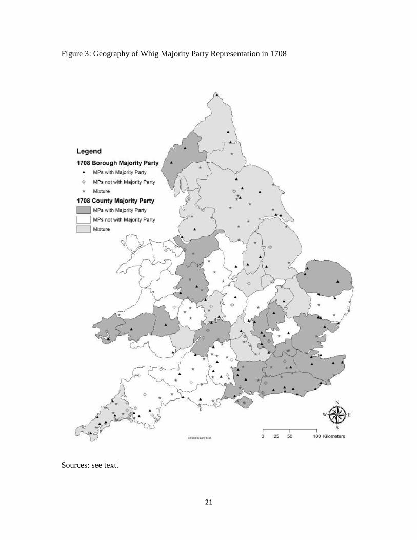
the number of majority party MPs across constituencies for every parliament. Figure 3 provides

an illustrative map of party classifications for the 1708 parliament when the Whigs were the

majority.7 In this and other parliaments, there was variation in majority party representation

across space with regions like the southeast tending to be more Whig.

7 Municipal Boroughs are cities indicated with symbols. Counties are outlined with white, light grey, or dark grey

backgrounds. The darkest boroughs or counties are where most MPs were with the Whig majority. A constituency

is considering to be well represented by the majority party if the fraction of MPs in the majority is above 0.8. A

constituency is not well represented if the fraction of MPs in the majority party is below 0.2. The consistency has

mixed representation if the fraction of MPs in the majority party is in-between 0.2 and 0.8.

21

Figure 3: Geography of Whig Majority Party Representation in 1708

Sources: see text.

22

The final step is the creation of spatial variables for town’s political characteristics based on

nearby constituencies. As I will justify shortly, the key explanatory variables for river acts are

the number of majority party MPs in the county of the candidate town and the number of

upstream and downstream majority party MPs in constituencies within 25 miles of a candidate

town. Other variables are the number of contests and incumbent MPs in upstream and

downstream constituencies within 25 miles.

The summary statistics are provided in table 3. Each cell pertains to one of 419 candidate

towns matched to one of the 14 parliaments spanning 1690 to 1741. The main outcome variable,

‘River Act,’ is an indicator for whether the town had a navigation act in that parliament. 51 out

of the 419 candidate towns got river navigation acts from 1690 to 1741 and no town had more

than one river act.8 As a result if the adopting town got a river act in a parliament they are

dropped from all subsequent parliaments. Note also that a single river act could apply to several

towns. In the estimation, I address the cross-sectional dependence between towns.

Another outcome variable is ‘River Bill,’ an indicator for whether the town had a navigation

bill introduced in that parliament. There were about two times as many river bills as river acts

indicating that the success rate for bills was around 50%. Later in the paper I will separately

analyze the factors affecting the introduction of bills and the success of bills once introduced.

The remaining variables incorporate political and economic characteristics of towns and

nearby towns and constituencies. To give two examples: (1) ‘Manufacturing’ is an indicator if

the town has manufacturing activity according to Blome and (2) ‘Manufacturing, Upstream &

8 Note also there are three towns that Blome records as having a harbor or having river navigation in 1670, but are

included in the candidate list because by 1690 they report in the Journals that their navigation had deteriorated due

to maintenance or changes in environmental conditions.

23

within 25 miles’ counts the number of towns with manufacturing activity that are upstream and

within 25 miles.

Table 3: Summary Statistics

Units: town-parliaments

n=5813 Adoption variables

mean st. dev. mean st. dev.

River Act 0.009 0.093 Previous Turnpike Acts

within 25 miles 45345 45345

River Bill 0.018 0.134 Previous Rivers Acts within

25 miles 45345 45345

Political variables

mean st. dev. mean st. dev.

Majority MPs upstream,

25 miles 4.426 3.65

Majority MPs downstream,

25 miles 3.854 3.057

Contests upstream, 25

miles 2.13 1.937

Contests downstream, 25

miles 1.869 1.639

Incumbent MPs

upstream, 25 miles 4.351 3.57

Incumbent MPs downstream,

25 miles 3.862 3.235

Majority MPs county 0.844 0.789

Town characteristics

mean st. dev. variable mean st. dev.

Manufacturing 0.211 0.408 Alms House 0.02 0.141

Mining 0.037 0.19 Local Government Officials 0.211 0.408

Harbor 0.008 0.09 Market Potential Local (000s) 16.801 9.086

Major Highway 0.632 0.482 Market Potential distant

(000s) 8.436 14.747

Coast or Navigable

River 0.002 0.049 Elevation Change (feet) 146.53 132.51

Free School 0.079 0.27 Distance to navigation head

(miles) 28.062 19.381

Southwest 0.208 0.406 Southeast 0.219 0.414

West Midlands 0.156 0.363 East Midlands 0.15 0.357

Wales 0.072 0.258 North 0.192 0.394

24

Characteristics all towns Up & within 25 miles

mean st. dev. mean st. dev.

Manufacturing 2.377 2.268 Local Government Officials 2.907 1.626

Mining 0.391 0.782 Market Potential Local

(00,000s) 2.82 3.844

Harbor 0.642 1.005 Free School 1.029 1.243

Major Highway 8.148 6.061 Alms House 0.327 0.687

Coast or Navigable

River 1.809 3.229

Characteristics all towns down & within 25 miles

mean st. dev. mean st. dev.

Manufacturing 2.341 2.17 Local Government Officials 2.507 1.518

Mining 0.386 0.697 Market Potential Local

(00,000s) 2.604 3.126

Harbor 0.408 0.751 Free School 0.871 1.154

Major Highway 8.308 5.856 Alms House 0.308 0.623

Coast or Navigable

River 1.583 2.644

IV. Identifying locations of Support and Opposition

The main explanatory variables in this paper are the number of upstream and downstream

majority party MPs within 25 miles. They are meant to capture the political connections of

locations where opposition and support to acts was most likely. A justification for this approach

comes from the evidence on petitions supporting and opposing bills found in the Journals of the

House of Commons. The petitions data is processed through several steps. The first is to classify

all petitions as supporting, opposing, or neither. Next, the stated locations of petitioners are

matched to the towns in Blome. Not all petitions could be matched because some groups came

from villages or rural areas not in Blome. There were 152 matched supporting petitions and 85

matched opposing petitions. The supporting petitions include the original petition that started the

25

bill. As a last step I compare the locations between supporting and opposing towns and the town

to whom the bill was matched. If there are multiple towns matched to the bill, I chose the most

upstream town to represent the bill’s location.

Figure 4 shows the distribution of the distances between supporting petitioners and the most

upstream towns associated with a river bill and the same for opposing petitioners. Supporting

petitioners are clustered at distance zero which means they were in the town with the river

navigation bill. There was support for river bills outside of the town too. In these cases, it

appears to be roughly uniform over a 40 mile span. Most of the opposing petitioners were

between 15 and 25 miles from the town with the river navigation bill.

Sources: see text.

0

5

10

15

20

25

30

35

0 5 10 15 20 25 30 35 40 >40

Fre

qu

ency

Distance in Miles

Figure 4: Petitioner's distance to towns with river

navigation bills

opposition support

26

There is another result that most supporting petitioners were upstream from the town with the

river navigation bill and most opposing petitioners were downstream. Earlier I discussed how

towns can be assigned to upstream and downstream areas using the direction between the

navigation head and the candidate town (see figure 2). It is arbitrary to assign the petitioners

from the candidate town to upstream and downstream areas, so I experiment with this definition.

Panel A of table 4 shows the counts in upstream and downstream areas for opposing petitions

and supporting petitions when the candidate town is included in the upstream. It is apparent that

opposition groups tended to be downstream and supporters tended to be upstream. The standard

t-test confirms that downstream status is significantly different in the two samples. Panel B

shows the counts when the candidate town is dropped. The same pattern applies. Opposition

groups tended to be downstream and supporters tended to be upstream.

Table 4: Opposition and Support for Bills in Upstream and Downstream towns

Panel A: when candidate town is upstream

opposition support

Upstream Downstream Upstream Downstream

Number of obs. 31 54 122 33

t-stat for hypothesis that mean for downstream dummy is same in opposing and

support sample -7.71

p-value

0

Panel B: when candidate town is dropped

opposition support

Upstream Downstream Upstream Downstream

Number of obs. 24 54 89 33

27

t-stat for hypothesis that mean for downstream dummy is same in opposing and

support sample -6.541

p-value 0

The patterns for support and opposition motivate my measurement of political connections.

As most opponents to a town’s river bill were downstream and within 25 miles of a town, the

political connections of likely opponents for a candidate town’s river act are measured by the

number of downstream majority party MPs or downstream incumbent MPs within 25 miles. As

most supporters were in the candidate town or were upstream some distance, the political

connections of likely supporters to a candidate town’s river act is measured by the number of

upstream majority party MPs or upstream incumbent MPs within 25 miles. The number of

majority party MPs in the county of the candidate town is also likely to reflect the political

connections of supporters as they tended to be located uniformly within 40 miles. The degree of

political competition in likely supporting and opposing areas is measured analogously by the

number of upstream and downstream constituencies with a contest in the previous election.

V. Estimation and Identification Strategy

The ‘baseline’ equation describing the diffusion of river acts across England and Welsh

towns is the following:

where the variable if candidate town i has a river act in parliament t and 0 otherwise,

is a vector of political characteristics in the town’s county, in upstream areas within 25

miles, and in downstream areas within 25 miles, is a vector containing the total

number of past river and turnpike acts for all towns within 25 miles after parliament , is

28

a town fixed effect, is a parliament fixed effect, and is the error term. In some

specifications, the time-invariant town characteristics are included when interacted with a time

trend. In the baseline model the standard errors are clustered on the town. Alternative estimates

for the standard errors are also shown.

Readers will note that the baseline model is a linear probability model. Although it is not

perfect, a linear probability model is a better alternative to the logit and probit models because it

easily allows for the inclusion of town and parliament fixed effects, which capture unobservable

factors.9 Later I incorporate a probit a model when analyzing the introduction of bills and their

success. The results are qualitatively similar to the linear model.

The key identification assumption is that political characteristics, like the number of

upstream and downstream majority party MPs, are exogenous conditional on the inclusion of

town fixed effects, parliament fixed effects, controls for past acts, and town-characteristic-

specific trends. While the controls address some unobservable factors, one could still argue that

time-varying unobservable factors contributed to the election of majority party MPs. Note there

are at least two channels of behavior behind this argument. The first channel is that supporters

who were considering the promotion of bills in the next parliament campaigned to get majority

party MPs elected. The second is that opposition groups campaigned to get majority party MPs

elected in order to improve their chances of rejecting a river navigation bill in a nearby town.

The second channel is the least plausible because opposition groups could not easily anticipate if

or when nearby towns would promote bills. Thus they could spend resources campaigning only

to find out that the candidate town never planned to promote a bill.

9 See Allison and Christakis (2006) for a discussion of fixed effects models for non-repeated events like technology

adoption.

29

The first channel is more plausible because supporters knew of their plans and thus could

take appropriate actions. The case of the river Avon bill suggests that this is not a theoretical

consideration. Recall that the inhabitants of Bath promoted the bill. The two MPs who first

presented the bill to the House of Commons were Trotman and Codrington, both of whom

represented Bath in the Commons and were part of the Tory majority in the 1710 to 1713

parliament. In the election leading up to 1710, one Bath MP, Codrington, was supported by the

Second Duke of Beaufort. The Duke is an important character because he is thought to have paid

the fees to introduce the river Avon bill (Hanham 2002). It would appear that Codrington was

elected in part to serve Beaufort’s interest in the Commons.

To address these endogeneity concerns I decompose changes in the number of majority party

MPs into two terms: one that is plausibly exogenous and the other that is potentially endogenous.

The sources of variation in majority party affiliation for all MP-seats (e.g. John Smith

representing Bedford borough) in the Commons between 1690 and 1740 are shown in table 5.

On average 23% of the MP-seats went from the majority party to out of the majority party

between parliaments and 24% of MP-seats went from out of the majority party to in the majority

party. What caused these changes? In the case where MP-seats went from the majority party to

out of the majority party, 49% (817 out of 1677) of the time there was a new majority party in

the Commons and the same MP was elected and remained affiliated with their party now in the

minority. The remaining reasons involve the election of new MPs or changes in incumbent MPs

party affiliation. There is a similar pattern for cases when MP-seats changed from out of the

majority to in the majority.

30

Table 5: sources of Variation in the Party affiliation of MP-Seats, 1690-1741

Number of MPs with seats at start of Parliament 7182

Number of MP seats that went from Majority Party to out of Majority Party 1677

Number of MP seats that when from out of Majority Party to with Majority 1689

Reasons for a seat going from Majority Party to out of Majority Party

Same majority party and new MP that is not with majority 366

Same majority party and same MP that is not with majority anymore 76

New majority party and new MP that is not with majority 418

New majority party and same MP that does not change to majority 817

Reasons for a seat going from not with Majority Party to with Majority Party

Same majority party and new MP with majority 348

Same majority party and same MP that changed to majority 136

New majority party and new MP that is with majority 353

New majority party and same MP now with majority 852

I use the constituencies where there was a new majority party in the Commons and the same

MP was elected and remained affiliated with their party as an exogenous source of variation for

changes in the majority party MPs near towns.10

The idea is that in these constituencies the skills

and party connections of MPs did not change, but because there was a change in the majority

party in the Commons beyond their control they experienced an exogenous change in majority

party connections. The next section reports the results for the baseline model and for several

extensions including specifications that test whether the number of majority party MPs is

endogenous.

VI. Results

10

More specifically, I calculate the change in majority party status for each MP-seat and then I calculate the change

that was exogenous and potentially endogenous as just described. Then I sum over the changes in MP-seats within a

20 or 25 mile distance of a town.

31

Table 6 shows the estimation results. Column 1 is the baseline and includes town and

parliament fixed effects. Column 2 adds region-specific time trends and town-characteristic-

specific time trends as controls. Column 3 is the same as 2 but adds a set of characteristic-

specific time trends for all upstream and downstream towns within 25 miles. Column 4 is the

same as 3 but reports Driscoll-Kraay standard errors which incorporate cross-sectional

dependence between towns (see Driscoll-Kray 1998, Hoechle 2007). Across all specifications,

having more majority party MPs in the county significantly raises the probability of river acts.

The opposite pattern is observed for majority party MPs downstream and within 25 miles. Here

the coefficient has a negative and significant sign in all specifications. Having more majority

party MPs upstream and within 25 miles raises the probability of river acts, but the coefficient is

not significant in the baseline model and when Driscoll-Kraay standard errors are reported. With

the exception of the last result, these results suggest that the adoption of river acts was indeed

affected by the political connections of likely supporters and opponents.

Other results in table 6 show that more incumbents within 25 miles had little influence as did

more upstream contests. On the other hand, having more contests downstream and within 25

miles significantly lowers the probability. The result suggests that political competition in areas

where opposition was more likely worked against river acts. Having more turnpike acts increases

the probability of a river act suggesting there was a complementarity between the two. There is

no significant complementarity between previous river acts nearby and current river acts.

32

Table 6: River Acts: baseline regressions

1 2 3 4

coeff. coeff. coeff. coeff.

Variables st. error st. error st. error st. error

Majority MPs, county 0.0046 0.0049 0.0047 0.0047

0.0021** 0.0021** 0.0021** 0.0026*

Majority MPs, up 25 miles 0.0011 0.0012 0.0015 0.0015

0.0007 0.0007* 0.0008** 0.001

Majority MPs, down 25 miles -0.0021 -0.002 -0.0021 -0.0021

0.0001*** 0.0007*** 0.0007*** 0.0008**

Incumbent MPs, up 25 miles 0.0001 0.0001 0 0

0.0005 0.0006 0.0006 0.0006

Incumbent MPs, down 25 miles 0.0008 0.0007 0.0005 0.0005

0.0005 0.0005 0.0005 0.0005

Contests, up 25 miles -0.0006 -0.0003 -0.0006 -0.0006

0.0011 0.0011 0.0011 0.0013

Contests, down 25 miles -0.0028 -0.0023 -0.0028 -0.0028

0.0012** 0.0011* 0.0012** 0.0016*

Previous turnpike acts, 25 miles 0.0014 0.0019 0.0025 0.0025

0.0007** 0.0008** 0.0008*** 0.0011**

Previous river acts, 25 miles 0.0039 0.0041 0.0032 0.0033

0.0028 0.0031 0.0031 0.0049

Parliament and town fixed effects yes yes yes yes

Region and town-characteristic trends no yes yes yes

town-characteristics trends, 25 miles no no yes yes

Driscoll-Kraay standard errors no no no yes

N 5813 5813 5813 5813

R-square 0.007 0.01 0.011 0.04

Notes: Standard errors are clustered on towns. *,**, and *** represent statistical significance at

the 1%, 5% and 10% level.

33

Endogeneity Concerns

As noted earlier I decompose changes in the number of majority party MPs into two terms:

one that is exogenous and the other that is potentially endogenous. The exogenous changes come

from parliaments where there was a new majority party in the Commons and in constituencies

where the same MP was elected and remained affiliated with their party. It is exogenous because

the constituency did not control who was the majority party and it did not elect a new MP to

influence its affiliation with the majority party. To make use of this information, I analyze a

‘differences’ version of the baseline model. In the case of river acts, the differences model is

where is the change in town i’s river act outcome from parliament t-1 to t,

is a vector representing the change in majority party MPs at the county or in

nearby constituencies from parliament t-1 to t, is defined analogously, and

includes regional indicators, economic characteristics for the town, and characteristics for all up

and downstream towns within 25 miles. I estimate three versions of this model. The first is OLS

and is potentially biased. The second is IV where is instrumented with the

exogenous component. The third is a reduced form of the IV model and includes only the

exogenous component of .

The results are reported in table 7. In OLS the three variables for changes in majority party

MPs have the expected sign, but none is statistically significant. In the IV model, the coefficients

for changes in county majority MPs and upstream majority MPs within 25 miles decrease

significantly in magnitude. However, in the IV model the coefficient for changes in downstream

majority party MPs within 25 miles is similar and in fact increases slightly to become

34

statistically significant (albeit at the 10% level only). In fact, the chi-square test implies that I

cannot reject the hypothesis that the change in downstream majority party MPs within 25 miles

is exogenous. In the last model the conclusions are similar. The exogenous component of the

change in downstream majority party MPs within 25 miles is similar in magnitude and

statistically significant. Variables for the change in county and upstream majority party MPs are

not significantly related to river acts.

Table 7: River Acts: OLS and IV models for differences specification

(1) (2) (3)

OLS IV

Exogenous

component only

coeff. coeff. coeff.

Variables st. error st. error st. error

Change Majority MPs, county 0.0016 0 0

0.0016 0.0017 0.0016

Change Majority MPs, up 25 miles 0.0008 0.0001 0.0001

0.0006 0.0006 0.0006

Change Majority MPs, down 25 miles -0.001 -0.001 -0.0011

0.0006 0.0006* 0.0006*

Change previous turnpike acts, 25 miles 0.0013 0.0013 0.0013

0.0009 0.0009 0.0009

Change Previous river acts, 25 miles 0.0131 0.0129 0.013

0.0070* 0.007* 0.0069*

Parliament FE, region FE, town characteristics,

characteristics for all up and downstream towns yes yes yes

N 5378 5378 5378

First Stage

Cragg-Donald Wald F statistic 1737.97

Endogeneity Test: Change Majority MPs, down 25 miles

35

Chi-sq(1)

0.626

P-value 0.429

Notes: Standard errors are clustered on towns. *,**, and *** represent statistical significance at

the 1%, 5% and 10% level.

Based on these results it would appear that OLS is biased upwards for variables measuring

the political connections of likely supporters to river acts. The most likely explanation is that

supporters campaigned for majority party MPs in order to assist in getting river bills passed. On

the other hand, OLS does not appear to be biased for variables measuring the political

connections of likely opponents to river acts. Opponents had a more difficult time campaigning

for majority party MPs to reject bills because they did not know when such bills would be

introduced. As a result, they might needlessly expend resources with little gain.

Further Robustness Checks

In the previous models, majority party strength is measured at 25 miles because petitioner’s

opposing river bills were generally within 25 miles from candidate towns. While there is good

justification for using 25 miles in the estimation other distance scales could give different results.

To check this, the model was re-run replacing variables measured at 25 miles with variables

measured at 20 miles or 30 miles. The results are shown in table 8. The specification is the same

as column 3 in table 6. It includes town and parliament fixed effects, region specific time trends,

town characteristic specific time trends, and characteristic specific trends for all towns upstream

and downstream. For comparison the results where variables are measured at 25 miles are also

reported in the first column. As might be expected the coefficients change in magnitude when

variables are measured at 20 or 30 miles, but they do not change in terms of statistical

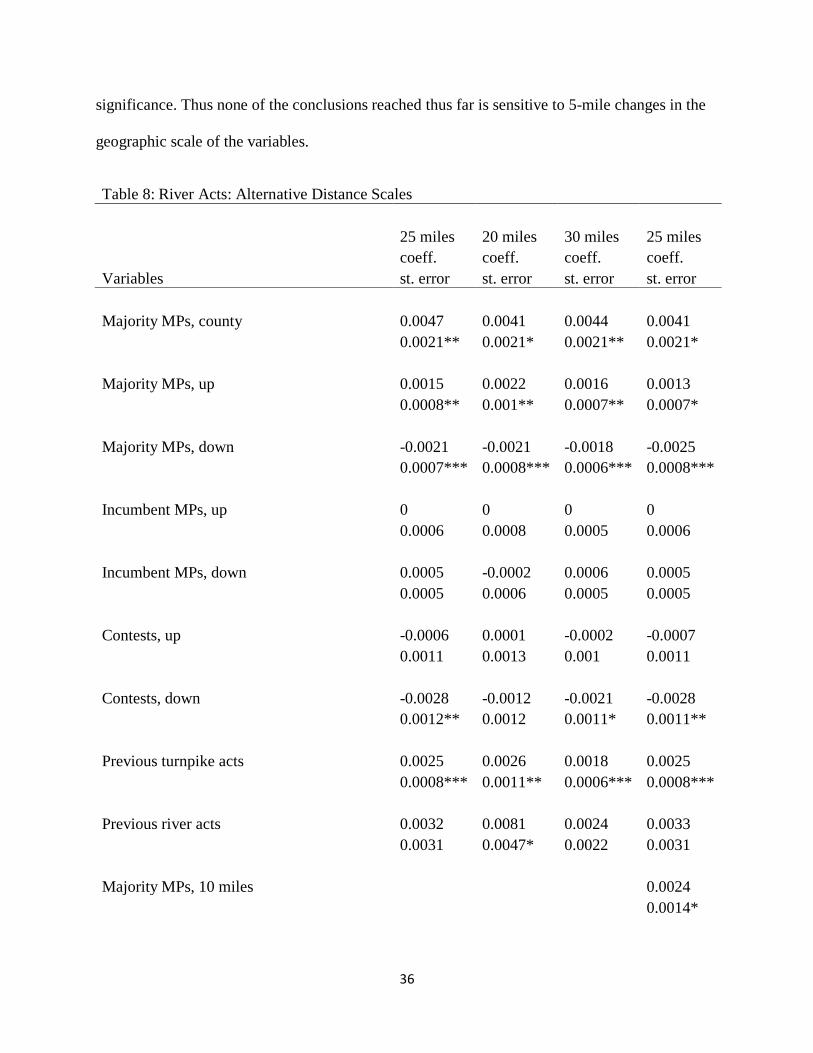
36

significance. Thus none of the conclusions reached thus far is sensitive to 5-mile changes in the

geographic scale of the variables.

Table 8: River Acts: Alternative Distance Scales

25 miles 20 miles 30 miles 25 miles

coeff. coeff. coeff. coeff.

Variables st. error st. error st. error st. error

Majority MPs, county 0.0047 0.0041 0.0044 0.0041

0.0021** 0.0021* 0.0021** 0.0021*

Majority MPs, up 0.0015 0.0022 0.0016 0.0013

0.0008** 0.001** 0.0007** 0.0007*

Majority MPs, down -0.0021 -0.0021 -0.0018 -0.0025

0.0007*** 0.0008*** 0.0006*** 0.0008***

Incumbent MPs, up 0 0 0 0

0.0006 0.0008 0.0005 0.0006

Incumbent MPs, down 0.0005 -0.0002 0.0006 0.0005

0.0005 0.0006 0.0005 0.0005

Contests, up -0.0006 0.0001 -0.0002 -0.0007

0.0011 0.0013 0.001 0.0011

Contests, down -0.0028 -0.0012 -0.0021 -0.0028

0.0012** 0.0012 0.0011* 0.0011**

Previous turnpike acts 0.0025 0.0026 0.0018 0.0025

0.0008*** 0.0011** 0.0006*** 0.0008***

Previous river acts 0.0032 0.0081 0.0024 0.0033

0.0031 0.0047* 0.0022 0.0031

Majority MPs, 10 miles

0.0024

0.0014*

37

Parliament & town FE, all characteristic

specific trends yes yes yes yes

N 5813 5813 5813 5813

R-square 0.012 0.013 0.012 0.012

Notes: Standard errors are clustered on towns. *,**, and *** represent statistical significance at

the 1%, 5% and 10% level.

The last specification in table 8 reveals a result of additional interest. It has the 25 mile scale

as in the baseline model but now the number of majority party MPs within 10 miles is added as

an additional variable. The results show that conditional on all other variables, having more

majority party MPs within 10 miles raises the probability of a river act (albeit at a marginal

statistical significance). This variable could reflect the political connections of river bill

supporters who tended to be very close to the candidate town and thus were within 10 miles.

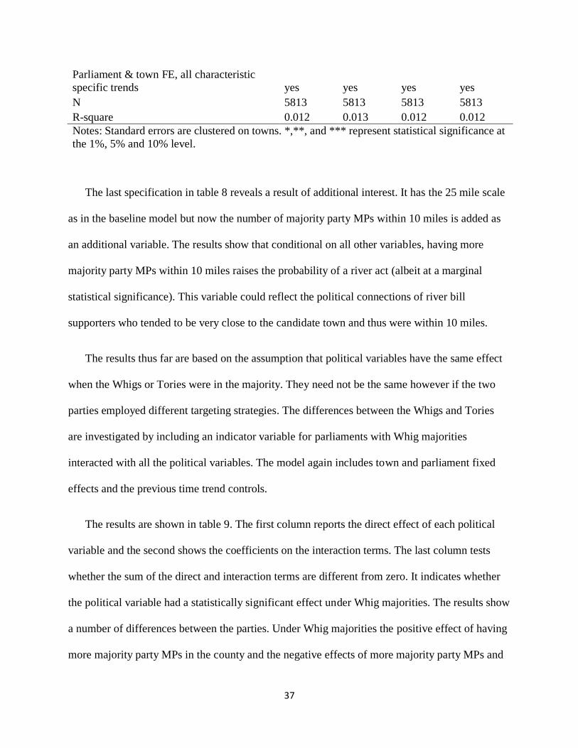
The results thus far are based on the assumption that political variables have the same effect

when the Whigs or Tories were in the majority. They need not be the same however if the two

parties employed different targeting strategies. The differences between the Whigs and Tories

are investigated by including an indicator variable for parliaments with Whig majorities

interacted with all the political variables. The model again includes town and parliament fixed

effects and the previous time trend controls.

The results are shown in table 9. The first column reports the direct effect of each political

variable and the second shows the coefficients on the interaction terms. The last column tests

whether the sum of the direct and interaction terms are different from zero. It indicates whether

the political variable had a statistically significant effect under Whig majorities. The results show

a number of differences between the parties. Under Whig majorities the positive effect of having

more majority party MPs in the county and the negative effects of more majority party MPs and

38

contests downstream are all greater in magnitude. Also there is a positive effect of having more

incumbents downstream under Whig majorities, but there is no effect of downstream incumbents

under Tory majorities.

Table 9: River Acts: Baseline with Whig Majority Interactions

Direct Effect

Interaction with

Whig Majority

Hypothesis test: direct

+ interaction effect=0

coeff. coeff. F stat

Variables st. error st. error P-value

Majority MPs, county 0.0026 0.0039 3.07

0.0028 0.0051 0.08

Majority MPs, up 25 miles 0.0015 -0.0002 1.83

0.0009* 0.0011 0.177

Majority MPs, down 25 miles -0.0015 -0.0011 8.9

0.0009 0.0011 0.003

Incumbent MPs, up 25 miles -0.0005 0.0014 1.45

0.0006 0.0007** 0.229

Incumbent MPs, down 25

miles -0.0003 0.0017 4.16

0.0006 0.0009* 0.042

Contests, up 25 miles 0.0006 -0.0022 1.19

0.0012 0.0015 0.277

Contests, down 25 miles -0.0013 -0.0027 7.73

0.0013 0.0014* 0.006

Previous turnpike acts, 25

miles 0.0027

0.0008***

Previous river acts, 25 miles 0.0031

0.0031

39

Parliament & town FE, all characteristic specific trends yes

N 5813 R-square 0.012

Notes: Standard errors are clustered on towns. *,**, and *** represent statistical significance at

the 1%, 5% and 10% level.

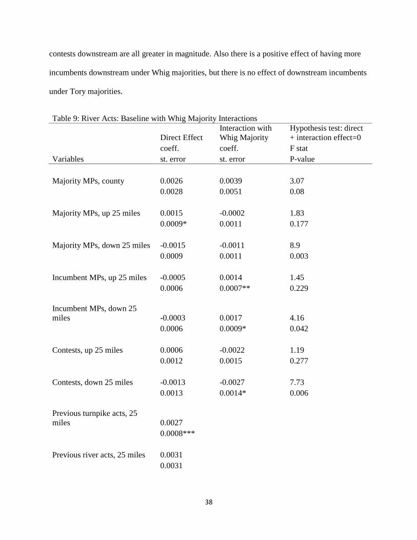
The quantitative difference between the two majority parties is illustrated in table 10. It

shows the effects of increasing various downstream variables relative to the mean probability

that a town got a river act. For example, in the upper left hand box the numbers imply that a town

was 13.6% less likely to get a river act relative to the mean if there was a Whig majority and it

had one more majority party MP, one more incumbent, but the same number of contests

downstream and within 25 miles. What is most notable is the large quantitative effects of

contests under Whig majorities. It appears that Whig majorities were more susceptible to the

effects of political competition. One explanation is that the Whigs were more effective in

targeting their policies to gain votes. Interestingly they appear to be targeting vested interests

more aggressively, which goes against theories that Whig majorities were pro-economic

development compared to Tory majorities.11

While there are differences between Whig and Tory majorities, it would be an over-statement

to argue that the two parties implemented very different strategies. Notice that having more

majority party MPs downstream lowered the probability of an act under both party majorities.

The same is true of downstream contests. Therefore, many of the same patterns of political and

economic behavior were present under the Whig and Tory majorities.

11

It has been argued that the rise of the Whig party following the Glorious Revolution was especially important for

Britain’s development. The Whigs are claimed to be more pro-development than the Tories by fostering a

manufacturing and financial sector (Pincus 2009, Pincus and Robinson 2012, Dudley 2013) and by providing a

stronger commitment to protect bondholder rights (Stasavage 2005).

40

Table 10: Differences in the effect of Downstream Political Connections and Contests under

Whig and Tory Majorities

Same # Contests

1 more contest

Whig Majorities

Whig Majorities

Same #

majority MPs

1 more

majority MP

Same #

majority MPs

1 more

majority MP

Same #

Incumbents 0 -0.296

Same #

Incumbents -0.456 -0.752

1 more

Incumbent 0.16 -0.136

1 more

Incumbent -0.296 -0.592

Tory Majorities

Tory Majorities

Same #

majority MPs

1 more

majority MP

Same #

majority MPs

1 more

majority MP

Same #

Incumbents 0 -0.171

Same #

Incumbents -0.148 -0.319

1 more

Incumbent -0.034 -0.205

1 more

Incumbent -0.182 -0.353

Notes: the effects come from the coefficients in table 9. They are divided by 0.0088, the

unconditional probability of a river act.

VII. Behavioral Mechanisms

The results show a strong negative relationship between the political connections of likely

opponents and the diffusion of river acts. What type of behavior can explain this outcome? In

this final section, I examine the promotion of river navigation bills across towns, the success of

river bills in the Commons, and the relationship between river bills and the electoral success of

the majority party in constituencies where opposition was most likely.

In order for a town to get a river navigation act someone had to petition for a river navigation

bill. The decision to ‘promote’ a bill was presumably carefully thought out as it involved

41

significant time and expense. One possibility is that promoters were rational, informed, and

forward looking. They understood how political connections influenced the likelihood of their

bill’s success and they were informed about the connections of likely supporters and opponents.

Promoters understood how lobbying would influence the likelihood of success and they

anticipated how much lobbying supporters and opponents would undertake. In short, they took

all of these factors into account when making the decision to promote a river navigation bill.

Another possibility is that promoters did not understand how political connections influenced the

success of their bill in parliament or they were misinformed about the connections of others.

They might have also failed to anticipate how much lobbying would occur. In this view of the

world, promoters only considered the likely financial returns to projects once approved, and not

the political factors that would influence a bill’s success in Parliament.

A simple model can illustrate these possibilities. Suppose the promoter has an exogenously

given expected financial return b if the project is approved and completed. To get approved, the

promoter needs to pay a fixed processing cost F and their bill needs to succeed in Parliament.

Supposing that a bill is introduced, let its probability of success be

, where

measures the political connections of the promoter, measures the political connections of the

opposition, is lobbying in favor of the promoter’s bill, is lobbying by the opposition

against the bill, and represents the baseline probability of success when political connections

and lobbying are zero. Notice that higher lobbying by the opposition or greater political

connections for the opposition lower the bill’s probability of success. The promoter is assumed

to have a belief about their bill’s probability of success which may differ from reality because of

misinformation about connections, lobbying, and their effects. Let the promoter’s belief for their

42

bills probability of success be

, where all previous variables are the

same and is an indicator function that equals 1 if the promoter has the correct belief about

political connections and 0 otherwise. is the promoter’s expectation about how much

lobbying will be done by supporters and is their expectation about how much lobbying

will be done by opponents. Notice that if the promoter has the correct beliefs and rational

expectations about lobbying then , otherwise .

The next step is to consider the promoter’s decision to introduce a bill. They will do so if

their expected gain exceeds the fixed cost F. In the case that the promoter has incorrect

beliefs about political connections then they will introduce the bill if

. Here political connections will not influence their decision. Instead what matters

are the projects expected financial returns , fixed costs F, and the expected lobbying amounts

and . In the case that the promoter has correct beliefs then they will introduce the bill

if + . Here greater political connections by

opposition groups will decrease the likelihood that the promoter introduces the bill and greater

political connections by supporters will increase the likelihood.

In the data I can easily examine whether political connections influenced the introduction of

river bills by running the same regressions as before except replacing the river act outcome

variable with an indicator for whether a town had a river bill introduced in that parliament. The

results are reported in column 1 in table 11. It is the same specification as the river act regression

in table 6 that includes all controls including town fixed effects, parliament fixed effects, region

specific trends, and all town characteristic specific time trends. Interestingly none of the

variables for political connections has a significant effect on the probability of a river bill being

43

introduced in a town. The only result that carries over from the river act model is that having

more contests downstream and within 25 miles lowers the likelihood of a river bill. Drawing on

the theoretical model above, it appears that promoters did not have the correct beliefs about

political connections.

It follows from the previous results that political connections must have influenced the

success of bills once introduced in Parliament. To investigate this channel, I estimate a probit

model where the probability of a bill’s success is a function of political variables along with the

number of opposing and supporting petitions matched to nearby towns. Recall that the matched

petitions were used earlier to identify the locations of likely supporters and opposition groups.

Here I use them as proxies for the amount of lobbying by supporters and opponents. Note that

there is a potential problem in analyzing the success of bills because unobservable factors

correlated with political variables might influence which bills got introduced and thus bias the

estimates. There is another potential problem in that supporting and opposing petitions are

endogenous. I deal with this in two ways. First, I estimate a Heckman selection equation for bills

along with a probit equation analyzing the determinants of a bill’s success. Second, in a standard

linear probability model I instrument for the number of opposing and supporting petitions using

characteristics for towns, for downstream towns within 25 miles, for upstream towns within 25

miles along with region fixed effects and parliament fixed effects. Neither solution is perfect.

The Heckman selection equation for whether a town has a river bill introduced includes the main

political variables, town characteristics, characteristics for towns upstream and downstream

within 25 miles, region fixed effects, and parliament fixed effects. It cannot include town fixed

effects because convergence in the likelihood could not be achieved otherwise. In the IV model,

the instruments for supporting and opposing petitions are weak and over-identification tests do

44

not provide strong evidence that they should be excluded. Despite the flaws in these two

approaches, they still provide some insights on the role of political connections, which is the

main focus here.

The results are reported in columns 2 to 4 in table 11. In column 2 the estimates from a

standard probit model show that having more majority party MPs downstream and within 25

miles significantly lowers the probability of a bill’s success. The same pattern holds in the

Heckman selection model in column 3. In fact, the coefficients are nearly identical. One reason is

that there is no evidence for a selection effect of bills as noted by the insignificant estimate of

rho.12

The IV linear probability model in column 4 yields the same finding for majority party

MPs downstream and within 25 miles. Therefore, the general conclusion is that the main channel

by which the political party connections of likely opponents influenced the adoption of river acts

was through the approval process in Parliament and not through the selection of bills.

There are two other results of interest in table 11. First, having more incumbents upstream

and within 25 miles increased a bill’s probability of success, although the coefficient is

marginally significant in two specifications and marginally insignificant in the other. Second

more petitions opposing a bill lowered its likelihood of success and more petitions supporting

increased its likelihood of success. This result is expected, but complicated to interpret given the

potential endogeneity of lobbying.

12

The results from the Heckman selection equation are not reported and are available upon request. The results

appear reasonable. For example, towns with greater elevation changes have a lower likelihood of a river bill and

towns with manufacturing and with greater market potential have a greater likelihood.

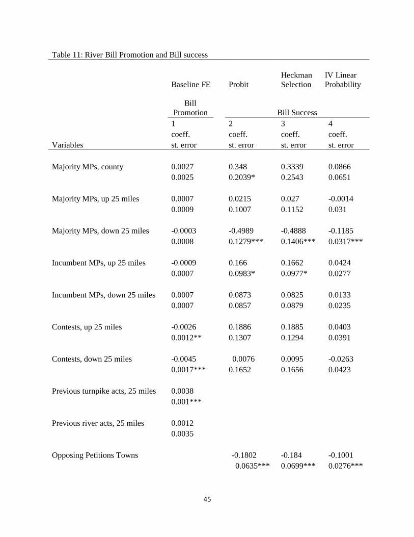
45

Table 11: River Bill Promotion and Bill success

Baseline FE Probit

Heckman

Selection

IV Linear

Probability

Bill

Promotion

Bill Success

1

2 3 4

coeff.

coeff. coeff. coeff.

Variables st. error st. error st. error st. error

Majority MPs, county 0.0027

0.348 0.3339 0.0866

0.0025

0.2039* 0.2543 0.0651

Majority MPs, up 25 miles 0.0007

0.0215 0.027 -0.0014

0.0009

0.1007 0.1152 0.031

Majority MPs, down 25 miles -0.0003

-0.4989 -0.4888 -0.1185

0.0008

0.1279*** 0.1406*** 0.0317***

Incumbent MPs, up 25 miles -0.0009

0.166 0.1662 0.0424

0.0007

0.0983* 0.0977* 0.0277

Incumbent MPs, down 25 miles 0.0007

0.0873 0.0825 0.0133

0.0007

0.0857 0.0879 0.0235

Contests, up 25 miles -0.0026

0.1886 0.1885 0.0403

0.0012** 0.1307 0.1294 0.0391

Contests, down 25 miles -0.0045

0.0076 0.0095 -0.0263

0.0017*** 0.1652 0.1656 0.0423

Previous turnpike acts, 25 miles 0.0038

0.001***

Previous river acts, 25 miles 0.0012

0.0035

Opposing Petitions Towns -0.1802 -0.184 -0.1001

0.0635*** 0.0699*** 0.0276***

46

Supporting Petitions Towns 0.1543 0.1546 0.0645

0.0702** 0.0701** 0.0283**

parliament & town FE, all town

characteristic specific trends yes

rho

P-value for Wald test of indep. eqns. (rho = 0) 0.8818

First Stage

Cragg-Donald Wald F statistic

1.019

Hansen's J Statistic for overidentification 58.914

P-value for Hansen's J Statistic

0.0657

N 5813

107 107 107

R-square or Pseudo R-square 0.016 0.27

Notes: Standard errors are clustered on towns. *,**, and *** represent statistical significance at

the 1%, 5% and 10% level. The instruments for supporting and opposing petitions in column 4

are characteristics for towns, characteristics for downstream towns within 25 miles,

characteristics for upstream towns within 25 miles, region fixed effects, and parliament fixed

effects

The significance of political party connections in the approval of bills within Parliament

suggests that party leaders were pursuing a targeting strategy. As noted earlier, there is a theory

that majority parties target legislative benefits to core supporters in order secure their support in

elections (Cox and McCubbins 1986). In this setting, the idea is that majority party leaders

targeted rejections to the opponents of river bills when the majority party was well represented in

their area because they wanted to retain opponent’s electoral support. If party leaders behaved

this way then one would expect that the success of the majority party in the next election would

be better in downstream areas if they rejected river bills and worse if they approved bills. To test

this theory I analyze a variable for the electoral outcomes for the majority party in downstream

areas. It equals the number of MPs gained or lost by the majority party from the last election if it

47

maintained the majority in the Commons. If there is a new majority party then electoral

outcomes equals the number of majority party MPs in the previous parliament minus the number

of majority party MPs in the current parliament.13

The second term is a proxy for the number of

MPs that the previous majority party gained or lost to the new majority party. I am interested in

majority party electoral outcomes only near towns where a river bill was introduced in the

previous parliament. The main variable of interest is an indicator for whether the river bill failed.

As I have argued throughout, the success or failure of a river bill is endogenous. To address this

issue, I instrument for the failure of river bills with the number of majority party MPs

downstream, upstream, and in the county in the previous parliament based on the fact that they

determined the success or failure of bills. In another specification I also include the number of

supporting and opposing petitions.

The results are reported in table 12. In column 1, OLS results show no significant effect from

the failure of a river bill. However, in columns 2 and 3 the IV results indicate that the failure of a

river bill significantly improves electoral outcomes for the majority party in downstream areas.

These results provide a strong clue as to why the majority party was targeting the opponents of

river bills. It helped them maintain their majority. In other words, there were electoral

consequences to ignoring the power of vested interests. Were there any electoral gains from

targeting the supporters of river bills? The answer is no. An unreported regression explaining

majority party electoral outcomes upstream shows no relationship with failed river bills.

13

More specifically Downstream majority party electoral outcomes near town i between parliament t and t-1 is equal

to (Majority MPs, down 25 miles (Majority MPs, down 25 miles -1) if there is no change in the majority

party and (Majority MPs, down 25 miles Majority MPs, down 25 miles ) if there is a change in the

majority party.

48

Table 12: Majority Party Electoral Outcomes Downstream and the Rejection of River Bills

OLS IV IV

1 2 3

coeff. coeff. coeff.

Variables st. error st. error st. error

River bill failed in previous parliament 0.1368 2.9321 2.1263

0.4304 1.322** 0.973**

Whigs Previous Majority Party 0.0189 0.924 0.6631

0.596 0.7232 0.5956

Change in majority party -0.0158 -0.5051 -0.3641

0.5152 0.5985 0.5354

MPs, down 25 miles 0.1498 0.2259 0.2039

0.085* 0.0822*** 0.0768***

Contests, down 25 miles -0.3135 -0.5938 -0.513

0.2102 0.2673** 0.2307**

regional FE yes yes yes

First Stage

Cragg-Donald Wald F statistic 7.436 6.548

Hansen's J Statistic for over-identification 0.937 4.712

P-value for Hansen's J Statistic 0.626 0.3181

N 92 92 92

R-square or Pseudo R-square 0.204

Notes: Standard errors are clustered on river bills. *,**, and *** represent statistical

significance at the 1%, 5% and 10% level. The instruments in column 2 are the number of

majority party MPs downstream, upstream, and in the county in the previous parliament.

Column 3 adds instruments for the number of supporting and opposing petitions.

49

VIII. Conclusion

There were remarkable changes in Britain’s political system after the Glorious Revolution. One

of the most important was the emergence of a competitive two party system. The Whigs and

Tories traded places as the majority party in the House of Commons seven times between 1690

and 1721. At the same time Britain embarked on many new policies, including the establishment

of river navigation companies which extended the waterway network. In this paper, I study

whether political party connections of vested interests influenced the diffusion of river

navigation acts. The empirical analysis shows that the extension of navigation to a town was less

likely when opponents of projects had more representation by the majority party in the

Commons. I also show that political party connections affected the success of bills in parliament

but not the selection of which bills got introduced. Lastly, I provide evidence that the rejection of

river bills contributed to better electoral outcomes for the majority party in areas where

opposition to river bills was more likely.

This paper contributes to the broader literature by identifying the effects of connections

to the majority political party in a novel way. There is a potential endoegenity problem in which

groups campaign to get majority party politicians elected in order to achieve legislative

outcomes. I address this issue by decomposing changes in the number of majority party MPs into

two terms: one that is exogenous and the other that is potentially endogenous. The exogenous

changes come from parliaments where there was a new majority party in the Commons and in

constituencies where the same MP was elected and remained affiliated with their party. The

estimation results show that the political party connections of supporters are endogenous but they

also show that the political party connections of opponents are likely to be exogenous allowing

for an identification of their effects.

50

In establishing this result, the paper provides the first rigorous evidence that political

party connections among vested interests can affect technology adoption. It complements the

literature showing that political parties affect economic outcomes in historical contexts and

today. It also complements the literature on vested interests, institutions, and the diffusion of

technologies. This literature is motivated by the stylized fact that poor countries are slower to

adopt best practice technologies and hence have lower productivity. Britain c.1700 was certainly

not a poor country relative to its neighbors, but like poor countries today its politics sometimes

slowed the adoption of legal technologies which Adam Smith believed were the greatest of all

improvements.

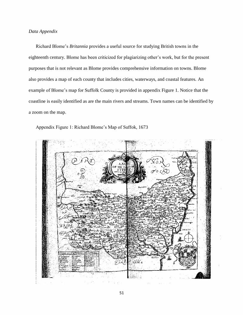
51

Data Appendix

Richard Blome’s Britannia provides a useful source for studying British towns in the

eighteenth century. Blome has been criticized for plagiarizing other’s work, but for the present

purposes that is not relevant as Blome provides comprehensive information on towns. Blome

also provides a map of each county that includes cities, waterways, and coastal features. An

example of Blome’s map for Suffolk County is provided in appendix Figure 1. Notice that the

coastline is easily identified as are the main rivers and streams. Town names can be identified by

a zoom on the map.

Appendix Figure 1: Richard Blome’s Map of Suffok, 1673

52

Source: Blome (1673).

Blome’s Britannia serves as a starting point for the analysis but it is necessary to supplement

with other data. Not surprisingly Blome did not know the population of towns when he wrote in

1673. Official census-data on town populations was not available until 1801. Nevertheless the

Cambridge Population History group has estimated the pre-1801 population of all parishes in

England and Wales using census-like sources. The Cambridge Population History group has

kindly provided their estimates of parish population in 1670 which I use to reconstruct the

population of cities listed in Blome. The latter are matched with parishes in the Cambridge data

and if necessary parishes are aggregated to form the boundaries of a town. Out of the 782 towns

in the Blome list, 717 were successfully matched with the Cambridge data. The population of the

remaining 65 towns was estimated using a model that predicts population from Blome’s

characteristics, most notably the amount of text he devotes to descriptions of each town.

The resulting town-level population data is to my knowledge the best that can be done with

current information. The population distribution across towns suggests that the estimates are

reasonable (see Appendix figure 2). The distribution is skewed to the right as is often the case

with modern data. Over half of the towns had a population under 1000 in 1670, while the mean

population is 1584. A few large cities like London pull the average population higher.

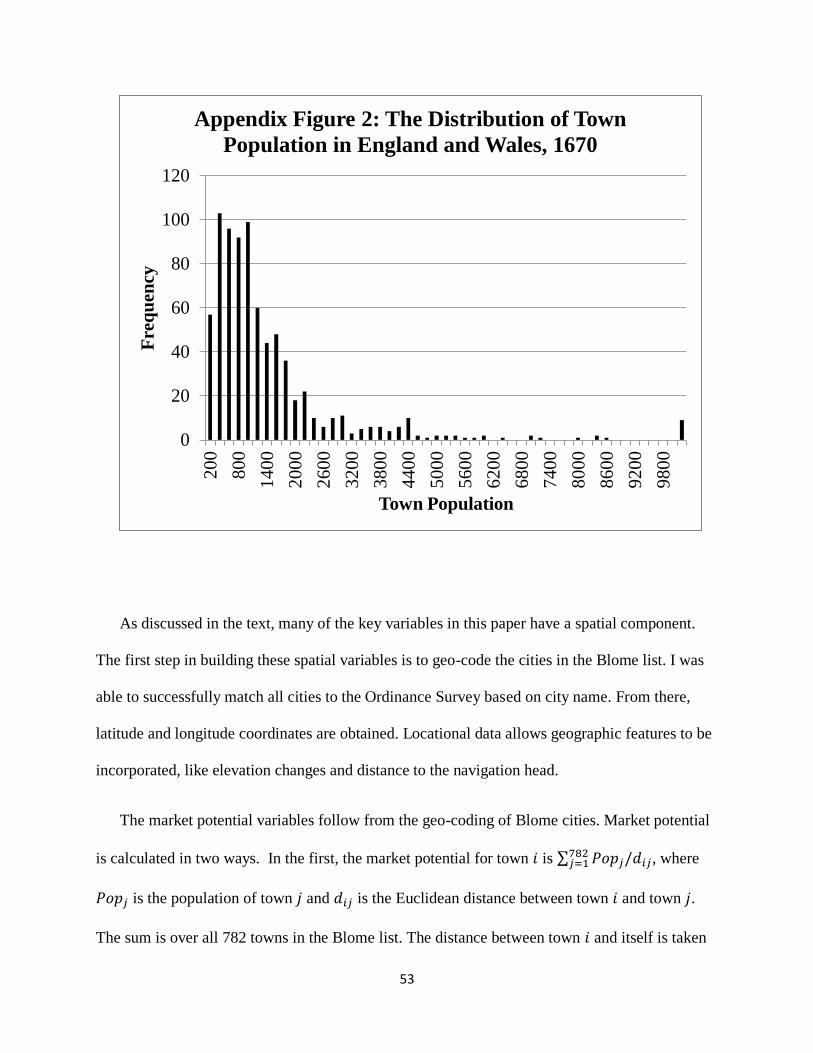
53

As discussed in the text, many of the key variables in this paper have a spatial component.

The first step in building these spatial variables is to geo-code the cities in the Blome list. I was

able to successfully match all cities to the Ordinance Survey based on city name. From there,

latitude and longitude coordinates are obtained. Locational data allows geographic features to be

incorporated, like elevation changes and distance to the navigation head.

The market potential variables follow from the geo-coding of Blome cities. Market potential

is calculated in two ways. In the first, the market potential for town is ∑ , where

is the population of town and is the Euclidean distance between town and town .

The sum is over all 782 towns in the Blome list. The distance between town and itself is taken

0

20

40

60

80

100

120

200

800

14

00

20

00

26

00

32

00

38

00

44

00

50

00

56

00

62

00

68

00

74

00

80

00

86

00

92

00

98

00

Fre

qu

ency

Town Population

Appendix Figure 2: The Distribution of Town

Population in England and Wales, 1670

54

to be √ following the convention adopted by Keeble et al. (1982). The first market

potential variable is meant to capture the size of nearby towns that could use the waterway

network. It is referred to as ‘market potential local.’

The second market potential variable captures the size of major cities that could be more

easily reached if the navigation project was completed. It is referred to as ‘market potential

distant.’ A major city is defined as a city with a population above 2500 in 1700 that was already

on the waterway network. The second market potential formula for town is ∑ ,

where is the population of major city and is the distance between town and

major city if the river navigation project was completed and a shipper followed the shortest

waterway transportation route. For this variable a GIS map of the waterway network in 1690 was

created including inland waterways and a coastal route. Then a network analysis tool was used

to calculate the distance from each town in the candidate list to major cities.

55

References

Albouy, David. “Partisan Representation in Congress and the Geographic Distribution of Federal Funds.”

Review of Economics and Statistics 95 (March 2013): 127–141

Allison, P. D. and N.A. Christakis, "Fixed Effects Methods for the Analysis of Non-Repeated Events,"

Sociological Methodology 36 (Summer 2006): 155-172.

Bellettini, Giorgio, Carlotta Berti Ceroni, and Giovanni Prarolo. "Knowing the right person in

the right place: political connections and resistance to change." Journal of the European

Economic Association 12 (2014): 641-671.

Besley, Tim, Torsten Persson and Daniel Sturm. “Political Competition and Economic

Performance: Evidence from the United States.” Review of Economic Studies, 77 (2010):

1329-1352.

Blanes i Vidal J, Draca M, Fons-Rosen C. “Revolving Door Lobbyists.” American Economic Review 102

(2012): 3731-48.

Blome, Richard. Britannia or a Geographical Description of the Kingdoms of England, Scotland, and

Ireland. London, 1673.

Bogart, Dan. “Did the Glorious Revolution Contribute to the Transport Revolution? Evidence from

Investment in Roads and Rivers,” Economic History Review 64 (November 2011): 1073-1112.

Bogart, Dan. “Whigs and Tories: Party Representation in English and Welsh Constituencies, 1690-1740.”

Working Paper 2014.

Bosker, Maarten, Buringh, Eltjo, and Jan Luiten Van Zanden. “The rise and decline of European

parliaments, 1188–1789," Economic History Review 65 (2012): 835-86.

Burgess, Robin, and Remi Jedwab, Edward Miguel, Ameet Morjaria, and Gerard Padró i Miquel. “The

Value of Democracy: Evidence from Road Building in Kenya,” NBER Working Paper No.

19398, 2013.

Carruthers, Bruce G. City of capital: Politics and markets in the English financial revolution. Princeton

University Press, 1999.

Cingano, F. and Pinotti, P. “Politicians at Work: the Private Returns and Social Costs of Political

Connections.” Journal of the European Economic Association, 11 (2013): 433–465.

Cox, Gary and Mathew McCubbins. “Electoral Politics as a Redistributive Game.” The Journal ofPolitics

48 (1986): 370–389.

56

Curto-Grau, Marta, Alfonso Herranz-Loncán, and Albert Solé-Ollé. "Pork-Barrel Politics in Semi

Democracies: The Spanish “Parliamentary Roads,” 1880–1914." The Journal of Economic

History 72 (2012): 771-796.

Comin, Diego, and Bart Hobijn. "Lobbies and technology diffusion." The Review of Economics

and Statistics 91 (2009): 229-244.

Cruickshanks, Eveline, Stuart Handley, and D.W. Hayton. 2002. The House of Commons 1690-1715.

Cambridge, 2002.

Defoe, Daniel. A Tour Through the Whole Island of Great Britain, 1724.

Dixit, Avinash and John Londregan. “The Determinants of Success of Special Interests in Redistributive

Politics.” The Journal of Politics 58 (1996): 1132–1155.

Dudley, Christopher. “Party politics, political economy, and economic development in early eighteenth

century Britain.” Economic History Review 66, (2013):1084-1100.

Driscoll, J. C., and A. C. Kraay. “Consistent Covariance Matrix Estimation with Spatially Dependent

Panel Data.” Review of Economics and Statistics 80 (1998): 549–560.

Faccio. M. “Politically Connected Firms.” American Economic Review 96 (2006): 369-386.

Faccio. M. McConnell, J.J., Masulis R. W. “Political Connections and Corporate Bailouts.” Journal of

Finance 61 (2006): 2597-2635.

Great Britain. Parliament. House of Commons. Journals of the House of Commons. London, 1803.

Hanham, Andrew. “Bath.” In The History of Parliament: the House of Commons 1690-1715, ed. D.

Hayton, E. Cruickshanks, S. Handley, 2002.

Harris, T. Politics Under the Later Stuarts: Party Conflict in a Divided Society 1660-1715. Longman,

1993.

Harris, Ron, Industrializing English Law: Entrepreneurship and Business Organization, 1720–1844.

Cambridge, 2000.

Hill, Brian W. The growth of parliamentary parties 1689-1742. Allen & Unwin, 1976.

Hoechle, Daniel. “Robust Standard Errors for Panel Regressions with Cross-Sectional Dependence.” The

Stata Journal, 7 (2007): 281-313.

Holmes, G. British Politics in the Age of Anne, rev. ed. London, 1987.

Hoppit, Julian, Failed Legislation, 1660-1800. London, 1997.

Horowitz, H. Parliament, Policy, and the Politics in the Reign of William III. Manchester, 1977.

Jayachandran S. “The Jeffords Effect.” Journal of Law and Economics. 49 (2006): 397-425.

57

Keeble D., Owens P. L. And Thompson C. “Regional accessibility and economic potential in the

European Community.” Regional Studies, 16 (1982): 419-32.

Lee, Frances E. "Geographic politics in the US House of Representatives: Coalition building and

distribution of benefits." American Journal of Political Science 47 (2003): 714-728.

Levitt, Steven D., and James M. Snyder. "Political parties and the distribution of federal outlays."

American Journal of Political Science 39 (1995): 958-980.

Lindbeck, Assar, and Jörgen W. Weibull. "Balanced-budget redistribution as the outcome of

political competition." Public choice 52.3 (1987): 273-297.

Mokyr, Joel. The lever of riches: Technological creativity and economic progress. Oxford

University Press, 1990.

Mokyr, Joel, and John VC Nye. "Distributional coalitions, the Industrial revolution, and the origins of

economic growth in Britain." Southern Economic Journal 74 (2007): 50-70.

Morden, Robert. The New Description and State of England, 1701.

Namier, Lewis Bernstein. The structure of politics at the accession of George III. London:

Macmillan, 1957.

North, D. C. and Weingast, B., “Constitutions and Commitment: The Evolution of Institutions Governing

Public Choice in Seventeenth-Century England.” The Journal of Economic History 49 (1989):

803-832.

North, D. C., Weingast, B. and Wallis, J. Violence and Social Orders: A Conceptual Framework for

Interpreting Recorded Human History. Cambridge 2009.

Parente, Stephen L., and Edward C. Prescott. Barriers to riches. MIT press, 2000.

Pincus, Steven. 1688: The First Modern Revolution. Yale 2009.

Pincus, Steven CA, and James A. Robinson. “What really happened during the glorious revolution?

NBER Working Paper No. 17206, 2011.

Sedgwick R. The House of Commons 1715-1754. Oxford, 1970.

Smith, Adam. An Inquiry Into the Nature and Causes of the Wealth of Nations. New York, 1976.

Speck, W. A. Tory and Whig: The Struggle in the Constituencies, 1701-1715. London, 1970.

Stasavage, D., Public Debt and the Birth of the Democratic State: France and Great Britain, 1688-1789

Cambridge, 2003.

Stasavage, D. “Partisan Politics and Public Debt: The Importance of the Whig Supremacy for Britain's

Financial Revolution," European Review of Economic History, 11 (2007): 123-153.

58

Voth, Hans-Joachim, and Thomas Ferguson. "Betting on Hitler-the value of political connections in Nazi

Germany." Quarterly Journal of Economics, 123 (2008): 101-137.

Walcott, Robert. English Politics in the Early Eighteenth Century. Oxford University Press, 1956.

Willan, T. S., River Navigation in England, 1600-1750. London, 1964.