Evidence and arguments for a four dimensional

spherical universe

Zulfikar Ahmed

September 11, 2012

1 Introduction

The idea that the universe has more than three dimensions goes back at least tothe nineteenth century, although I do not know of a careful scholarly study ofthe way in which the idea of higher dimensions is explicitly or implicitly presentin the thought of Riemann, for example, whose 10 June 1854 presentation, ”Onthe Hypotheses that lie at the foundation of geometry” introduced the notionof hyperspace. The belief that the universe has four macroscopic dimensionswas held by Rudolf Steiner, and Nietzsche believed that the apparent realityhides an unseen reality that he makes explicit from his earliest work, The Birthof Tragedy. Modern physical theories typically add microscopic dimensions forvarious technical reasons. In the early twentieth century, Gunnar Nordstrom,Theodor Kaluza, and Oscar Klein had independently proposed that electromag-netism and gravity can be unified by addition of a spatial dimension. We noteas well that William Hamilton spent his entire life from his first discovery ofquaternions obsessed with the idea that quaternions will revolutionize physics,and the four dimensional sphere is precisely the quaternionic projective line.

In this note, we take a view that we should have sharp observational evidencefor claims for a particular number of dimensions. We present arguments thatthe universe has precisely four macroscopic spatial dimensions, and that it is afour dimensional sphere. By 1973, a U(1) × SU(2) × SU(3) gauge theory hadsucceeded in uniting the electromagnetism and the nuclear forces. Beginningwith the description of the universe as a four dimensional sphere of fixed radius,we can note that the natural electromagnetism is SU(2) electromagnetism, thatproperties like spin are most likely effects from a four dimensional electromag-netism, and thus the natural conjecture that the nuclear forces are masking asingle force of SU(2) electromagnetism.

After giving well-known evidence whose parsimonious interpretation is amacroscopically four space dimensions from observed rotations of regular ar-rangements that cannot have translation invariance in three dimensions, whichhave been interpreted as quasicrystals, we sketch why macroscopic four spacedimensions would not lead to serious problems with the force law when the total

1

space of the universe is compact. Next we give an explanation of the redshiftas an artifact of treating waves on a sphere as waves on a flat space.

Two of the most promising features of a four sphere as a model of theuniverse are: quantization of inverse wavelengths are automatic on a spherewhere every geodesic is closed of the same length, and so quantization of energyis automatic; and second, that all functions and tensors on a sphere have waveaspects simply because the possibility of approximation by spherical harmonics.Wave-particle duality thus holds for any space localized object. These featuresare promising in their ability to infer quantum effects as consequence of theshape of the universe rather than as hypotheses on objects in the small scale.

The currently established model of elementary particles and their interac-tions is the Standard Model, which can be described as a gauge theory. Werecall the mathematical features of gauge theory. We are fortunate to be in asituation where detailed study of a classical field theory of SU(2) gauge the-ory on S4 had been done by physicists and mathematicians from the 1970s.Instantons for S4 were constructed by t’Hooft with 5k − 3 parameters quiteexplicitly and Atiyah, Hitchin, and Singer were able to calculate the dimensionof the selfdual moduli using the Atiyah-Singer index theorem to obtain 8k − 3,from which they could conclude that t’Hooft solutions did not describe all theinstanton solutions with topological charge k. Thus once the universe is knownto have a four spherical shape, we have some powerful results and analytic toolsfor S4 that we may use.

2 Arguments for naturality of three macroscopicspace dimensions

We follow J. D. Barrow‘s insightful article on dimensionality for historical con-text. From the commentary of Simplicius and Eustratius it is known thatPtolemy had written a study on the three dimensional nature of space enti-tled On dimensionality in which he argues that no more than three spatialdimensions are possible in Nature, but this has not survived. The question ofphysical relevance of spatial dimensions arises in an early work (1747) of Kant,who associated inverse square law of gravitation with three dimensions.

Ehrenfest wrote an article entitled, ’In what way does it become manifest inthe fundamental laws of physics that space has three dimensions?’ in 1917. Itexplained that stable planetary orbits, the stability of atoms and molecules, theunique property of wave operators and axial vector quantities are manifestationsof ’three dimensionality’ of space.

Note that if we restrict ’SM matter’, Standard Model matter, to be restrictedto lie in a three-dimensional hypersurface of a higher dimensional universe, thesearguments are no longer objections to existence of higher dimensions in nature.Furthermore, the argument I provide in a later section that the universe iscompact leads to different possible explanation of stability of planetary systemspossibly through the work on symplectic topology on periodic orbits of Hamil-

2

tonian flows – although S4 is not symplectic, it is the quaternionic projectiveline, and thus appears as the quotient of a symplectic manifold.

3 Observed symmetries of crystals show thatthe universe has at least four spatial dimen-sions

A basic result of crystallography is the crystallographic restriction theorem.This was first proved for arbitrary dimensions by R. Vaidyanathaswamy in 1928[10]. According to this theorem, crystals in three dimensions can have rotationalsymmetries of orders 1, 2, 3, 4, and 6. In four dimensions crystals can haveadditional symmetries 5, 8, 10 and 12. In six dimensions crystals can haveadditional symmetries 7, 9, 14, 15, 18, 20, 24, 30.

Since early 1980s when Daniel Shechtman first discovered crystal structures(deemed to be ’quasicrystals’ but which are much more simply explained ascrystals) with rotational symmetries of orders 5 and 10, there has not been asingle discovery of crystals with symmetries that would require six dimensions toexplain. For example, there has been no crystals found with sevenfold symmetry.

A crystal is modeled via mathematical lattices on Rn which are arrangementsof points that, relative to an arbitrarily chosen origin can be written as

r = k1a1 + · · ·+ knan

for a integers k1, . . . , kn and a1, . . . , an ∈ Rn. The lattices are translationallyinvariant. Although ’quasicrystals’ are not considered crystals,

• Their x-ray diffraction patterns have no qualitative difference from diffrac-tion patterns of ’ordinary’ crystals

• The standard models of ’quasicrystals’ are as slices of higher dimensionalcrystals. In other words the models we would use if we considered theseto be literally higher dimensional crystals are the same as the ones thatare used in practice

Observation of periodic arrangment with rotational symmetries of orders 5,8, 10, and 12 leaves us with two choices: either these are non-crystals and spaceis macroscopically three dimensional or they are crystals and space is macro-scopically higher dimensional. We can argue that parsimony would dictate thelatter as follows. If we observe a four dimensional crystal with a rotational sym-metry that cannot occur for a three dimensional crystal, then we cannot expectto observe three dimensional translation invariance for we might be observing anirrational slice. But we know that even in the case of Penrose’s aperiodic tiling,there is an algebraic theory of projections from higher dimensions [1] and thisis the case with quasicrystals generally. It then is simply a matter of semanticsto call such objects ’quasicrystals’. A purely parsimonious explanation of theobserved crystal symmetries of orders 5, 8, 10, and 12 is that the universe itself

3

has at least four macroscopic spatial dimensions. The parsimony argument isclearer when we weigh the added complexity introduced by a quasicrystal theoryto maintain three dimensions versus four dimensions and crystal theory.

Crystal structures are determined by diffraction of electrons, X-rays or neu-trons, and studying the interference of phase differences between rays elasticallyscattered from different atoms in the crystal.

In principle, we could discover crystals with 7 or 9 fold rotational symme-try leading us to conclude by this reasoning that the universe has at least sixmacroscopic spatial dimensions, but a vigorous search by crystallographers hasnot produced any such example in 30 years since Shechtman’s groundbreakingdiscovery.

4 Possible four dimensional vision

The pineal gland has characteristics of a visual organ according to, among oth-ers, the 1999 Science article of Lucas et. al. [6] on regulation of mammaliancircadian behavior by non-rod, non-cone, ocular photoreceptors. In 1992, Lol-ley et. al. [5] had studied signal transduction components in common betweenretina photoreceptors and pinealocytes of the pineal gland. These features areconsistent with the theory that the pineal gland could act as a visual organ forfour dimensional phenomena.

5 Implications of at least four dimensions

A parsimonious conclusion of at least four spatial dimensions is sufficient rea-son for us to reconsider the standard interpretations of the dominant physicaltheories, in particular of quantum mechanics which is numerically one of themost successful scientific theories to date. This is because intuitively at least,the basic reasons for discarding nineteenth century classical physics for quan-tum mechanics were the explanation of the observed blackbody spectrum whichwas resolved by Planck simply by introducing quantization of energy and ona four dimensional sphere since every geodesic is closed with the same length,quantization of frequency can be achieved whether we have a classical theory ora special quantum theory, and the second reason that a classical hydrogen atomwould be unstable because the electron orbiting a stationary proton would dowork and lose electromagnetic energy. This latter problem can find a simplesolution in a four dimensional sphere.

As an illustration of the issue of automatic quantization, recall that the stan-dard method of quantization is to replace energy by the operator i~∂/∂t. Notehere that ~ is simply the inverse of the length of a closed geodesic of an S4(1/h)-universe. Thus this quantization procedure is producing a linearization after arescaling. In the four-sphere context, on the other hand, classical physics con-tains quantized information without linearization. A natural hypothesis is thatthe physical three dimensional universe is isometrically immersed in S4(1/h)

4

and quantum mechanics arises as the linearization of a classical physical theoryon the tangent bundle TM .

If these claims are concretely illustrated, then we open up the possibilityof a classical physics on a four dimensional physics as a valid description ofthe actual universe. While such a conclusion might lead to a less sophisticatedphysical theory than currently held, we recall that the two criteria for rankingscientific theories that do fit the facts are parsimony and predictive power.

6 The universe must be compact

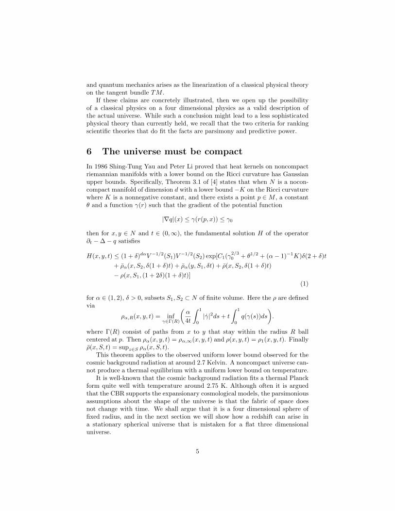
In 1986 Shing-Tung Yau and Peter Li proved that heat kernels on noncompactriemannian manifolds with a lower bound on the Ricci curvature has Gaussianupper bounds. Specifically, Theorem 3.1 of [4] states that when N is a nocon-compact manifold of dimension d with a lower bound −K on the Ricci curvaturewhere K is a nonnegative constant, and there exists a point p ∈M , a constantθ and a function γ(r) such that the gradient of the potential function

|∇q|(x) ≤ γ(r(p, x)) ≤ γ0

then for x, y ∈ N and t ∈ (0,∞), the fundamental solution H of the operator∂t −∆− q satisfies

H(x, y, t) ≤ (1 + δ)dαV −1/2(S1)V −1/2(S2) exp[C1(γ2/30 + θ1/2 + (α− 1)−1K)δ(2 + δ)t

+ ρα(x, S2, δ(1 + δ)t) + ρα(y, S1, δt) + ρ(x, S2, δ(1 + δ)t)

− ρ(x, S1, (1 + 2δ)(1 + δ)t)]

(1)

for α ∈ (1, 2), δ > 0, subsets S1, S2 ⊂ N of finite volume. Here the ρ are definedvia

ρα,R(x, y, t) = infγ∈Γ(R)

(α

4t

∫ 1

0

|γ|2ds+ t

∫ 1

0

q(γ(s))ds

).

where Γ(R) consist of paths from x to y that stay within the radius R ballcentered at p. Then ρα(x, y, t) = ρα,∞(x, y, t) and ρ(x, y, t) = ρ1(x, y, t). Finallyρ(x, S, t) = supz∈S ρα(x, S, t).

This theorem applies to the observed uniform lower bound observed for thecosmic background radiation at around 2.7 Kelvin. A noncompact universe can-not produce a thermal equilibrium with a uniform lower bound on temperature.

It is well-known that the cosmic background radiation fits a thermal Planckform quite well with temperature around 2.75 K. Although often it is arguedthat the CBR supports the expansionary cosmological models, the parsimoniousassumptions about the shape of the universe is that the fabric of space doesnot change with time. We shall argue that it is a four dimensional sphere offixed radius, and in the next section we will show how a redshift can arise ina stationary spherical universe that is mistaken for a flat three dimensionaluniverse.

5

7 The redshift can be explained as mistakingspherical waves by linear waves

First, recall that the redshift phenomenon is the following. When performingspectral analysis of a light from a distant object, we can detect absorption linesof abundant elements. For example, the absorption lines for hydrogen. Theexpected wavelength for the H-α line in the spectrum is 656.3 nanometers, butthe line observed in the spectrum of a distant object could appear at a longerwavelength. In 1929 Hubble discovered a remarkable linear relation betweenthe redshift of spectral lines and the distance of objects. Since then the redshiftdistance relation has been the central empirical foundation for expansionaryuniverse cosmological models. In this section we provide some observation ofhow a linear redshift would be expected in a stationary spherical universe wherethe electromagnetic waves are treated as linear waves.

The standard explanation for the redshift-distance relationship for distantgalaxies has been that this is a consequence of a Doppler effect. But there arealternative explanations for this phenomenon. Although our explanation of theredshift is different from the so-called ’tired light’ hypothesis of Fritz Zwicky,we mention it for historical context. A uniform loss of energy by signals fromdistant galaxies proportional to the distance travelled would result in a redshiftas well. The idea that the photons could lose energy as they travel is not newand is due to Swiss astronomer Fritz Zwicky who suggested the hypothesis in1929. The mechanism he proposed for loss of energy of photons due to loss ofmomentum to surrounding masses due to gravitational interactions ([13]) The”tired light” hypothesis has not been accepted with the major arguments againstit being that reducing photon energy would also change its momentum, blurringthe light which is not observed, that there is an observed time dilation wherea supernova that takes 20 days to decay appears to take 40 days to decay forredshift z = 1, and that the tired light cannot produce the observed blackbodyspectrum correctly, for example by arguments of Edward Wright ([?]). The lastof these arguments is open to criticism because cosmic background radiation isin thermal equilibrium and the tired light hypothesis pertains to signals fromdistant galaxies.

7.1 Possible explanation: treating frequency as n insteadof√

n(n + 3)

In this section we provide a concrete way in which a linear redshift is expected(of the same order as observed) when spherical waves are treated as waves on aflat space. This suggests that the redshift is not a physical phenomenon at allbut rather a systematic artifact of treating spherical waves as linear waves. Inparticular, there need be no energy loss that corresponds to the redshift at all,and no need for an expansionary model of the universe.

To clarify this terminology of spherical versus linear waves, we define linearwaves to be the solution of the wave equation on flat Euclidean spaces and

6

spherical waves to be the solutions of the wave equation on spheres. We areparticularly interested in the flat space R3 and the four-dimensional sphere S4.

The wave equation1

c2∂2u

∂t2−∆u = 0

can be solved on a four dimensional sphere of radius a by separation of variablesand an eigenvalue expansion in spherical harmonics. With

ωk =c

a

√k(k + 3)

the solution consists of linear combinations of terms of type

Φ(x)e(−iωkt),

where Φ(x) is a spherical harmonic with eigenvalue k(k + 3). The relationbetween wavelengths and frequencies in this case is not ν = c/λ but ratherν =

√n(n+ 3) when λ = c/n. There is no problem interpreting the term

involving√n(n+ 3) as a frequency because in the solution, it appears as a

coefficient of time in the circular function e−iωt.Let us consider what happens for the case of the H-α line at 656 nanome-

ters. Consider the distance of 1 light second, which is obviously many orders ofmagnitude larger than the wavelength of 656 nanometers. In this case

ν = 4.573171× 1014

and we can treat ν as an integer with negligible error.We are interested in seeing what happens in a distance of around 106 parsecs,

which is the unit of distance used by Hubble. The actual frequency will be√n(n+ 3), and the error per light second of the wavelength will be

c(1

n− 1√

n(n+ 3))

which will be a shift to longer wavelengths. The shift of 656 nm wavelengthover distance 106 parsecs would be around 0.023 nanometers, which is smallbut detectable. Now if we define z to be the ratio of this shift to the expectedwavelength of 656 nm and multiply z by the speed of light c we obtain 10,518km/s which is in the order of magnitude of the velocities that Hubble used inhis dataset.

We can check that the analysis above is sensible by a simple simulation. Wesample points on S4 uniformly, label 20

from cvxopt import normal , uniformfrom cvxopt . b l a s import nrm2from math import ∗N = 100n = 5

7

wl1 = 0.01wl2 = 0.0001

A = normal (n ,N)F = uniform (1 ,N)

f o r i in range (N) :A[ : , i ] = A[ : , i ] / nrm2(A[ : , i ] )

x = normal (n , 1 )x = x/nrm2( x )

r e d s h i f t s = i s r a d i o =

f o r i in range (N) :dot = ( (A[ : , i ] ) . t rans ( )∗ x ) [ 0 , 0 ]d = acos ( dot )

i f F [ i ] > 0 . 8 :wl = wl1i s r a d i o [ d ] = 1

e l s e :wl = wl2i s r a d i o [ d ] = 0

f r eq 1 = 1/wlf r eq 2 = s q r t ( f r eq 1 ∗( f r eq 1 +3))r e d s h i f t = (1/ f r eq1 − 1/ f r eq2 )∗d

r e d s h i f t s [ d ] = r e d s h i f t

f o r key in so r t ed ( r e d s h i f t s . keys ( ) ) :p r i n t key , r e d s h i f t s [ key ] , i s r a d i o [ key ]

The Steady State model of Hoyle, Gold, and Bondi was rejected for the BigBang model because astronomers believed that radio galaxies are older and theyhad a skew in distance compared to visible galaxies. The simulation here makesclear that this skew is expected for radio galaxies for the redshift. To the extentthat the distances of the radio galaxies was computed from their redshifts viathe ’Hubble relation’, the true distance distribution of these galaxies could wellbe indistinguishable from the distribution of visible galaxies.

The analysis above indicates that the observed redshift is quite likely ex-plained fully by electromagnetic waves being spherical waves in a four dimen-sional sphere, and in particular the redshift phenomenon does not necessicitatean expansion of the universe.

8

We can test this hypothesis that the redshift can be explained as an artifactof mistaking spherical waves as linear waves by checking such a model on amodern dataset containing measurements of distance and their redshifts. Wetook a dataset of these measurements for 957 cosmic objects from [?].

8 Avoiding the wrong force law

A basic reason for dismissing four macroscopic spatial dimensions is the ideathat in D macroscopic dimensions, the force laws would behave as 1/rD−1 whichfor a universe with four macroscopic spatial dimensions would lead to inconsis-tency with Newtonian physics. However, the reasoning that is used for Planckscale compactified dimensions, which the Kaluza-Klein theories propose can beextended to a macroscopic compact dimension as well.

Merag Gogberashvili had solved this issue for a noncompact extra dimensionin 1998 [?]. L. Randall and R. Sundrum [9] have written of how a model of a3+1 brane universe where the Standard Model localizes in a higher dimensionalspace where gravity operates avoids the problem of the wrong force law.

The hierarchy problem is the large gap between the Higgs mass, mEW ∼103GeV and the Planck mass MPl ∼ 1019GeV . Arkani-Hamed, Dvali, andDimopoulos [?] followed the following simple idea of overcoming this problemvia adding n compact dimensions of radius R. The Planck mass of this (4 + n)dimensional theory is taken to be ∼ mEW . Two test masses m1,m2 placedwithin a radius r << R will feel a gravitational potential

V (r) ∼ m1m2

M2Pl(4+n)

1

rn+1

and for distances r >> R the potential is

V (r) ∼ m1m2

M2Pl(4+n)R

n

1

r

The effective four dimensional MPl ∼M2+nPl(4+n)R

n. This strategy unfortunately

does not produce a useful answer with n = 1 for which setting MPl(4+n) ∼ mEW

and solving for R produces R ∼ 1013cm which would affect the force law in thesolar system scale.

In a D-dimensional space with one dimension compactified on a circle ofradius R, the line element is

dl2 = gijdxidxj = dr2 + r2dΩD−2 +R2dα2

with√g ∼ RrD−2. The force law derived from the potential that solves the

Laplace equation is

F ∼ GD2πRrD−2

= G/rD−2

where the constant has absorbed the effect of the extra dimension. Our proposalof a universe with four macroscopic spatial dimensions but a sphere of fixed

9

radius O(1/h) falls in this category as well, although the additional dimensionis not microscopic.

An interesting observation is that in the case of charged particles, the mag-nitude comparison of Coulomb versus gravitational forces give us the following

|Fem||Fgrav|

= 4.17× 1042

In the case that the gravitational force law in three macroscopic dimensions is aresult of four dimensional force, the gravitational constant G3 is a reduction ofa four dimensional gravitational constant G3 = G4/(2πR), which would changethe relative strengths of electromagnetic and Coulomb forces to the order 108

assuming that the Coulomb force strength remains constant.

9 Special features of four spatial dimensions

The following is material that is well-known to geometers and articulated byAtiyah and Hitchin in a 1978 paper. The basic idea is that electromagnetism isnaturally defined on four dimensional manifolds due to the fact that the Hodge*-operator maps 2-forms to 2-forms on a four dimensional manifold and thatthe curvature of a connection is a 2-form. These features do not exist for higherthan four dimensions.

One of the special features of four dimensional compact manifolds is thatthe rotation group SO(4) is locally Spin(4) = SU × SU(2). In fact, Spin(4)is the double-cover of SO(4). The differential 2-forms on a compact four di-mensional manifold decompose into self-dual and anti-self dual parts by theeigenspaces of the Hodge *-operator. Electromagnetism can be formulated on afour dimensional manifold by considering a principal SU(2)-bundle P and con-sidering the electromagnetic potential A to be a connection on P with curvatureF = dA satisfying the Yang-Mills equations which say that F is anti-self-dualas a 2-form.

10 Some criteria for isometric immersion of athree manifold in a four-dimensional sphere

The general necessary and sufficient conditions for a riemannian n-manifold tobe isometrically immersed into one of the space forms of dimension n + 1 arethe Gauss and Codazzi-Mainardi equations. A different type of necessary andsufficient conditions are given by M-A Lawn and Julien Roth [3]. Their conditionfor isometric immersion into a space form of curvature κ = 4η2 is the existenceof two spinor fields φ1 and φ2 of constant norm that satisfy the equations

Dφ1 = (3

2H + 3η)φ1

Dφ2 = −(3

2H + 3η)φ2

10

where H is a real valued function, which are equivalent to the equations in termsof the spin connection on M :

∇SMX φ1 =1

2A(X) · φ1 − ηX · π1

∇SMX φ2 = −1

2A(X) · φ1 + ηX · π2

with traceA = 2H. Either set of conditions then imply the existence of animmersion F : M → S4(κ) where κ stands for the curvature rather than theradius.

We have already given direct evidence that the universe is compact and fourdimensional. The Lawn-Roth result above is a promising method of showingthat an apriori three dimensional universe with two constant norm eigenspinorscan be used to isometrically immerse the universe in a four-sphere.

In order to make this idea concrete, consider the proxy for the physicaluniverse to be a 3-dimensional spin manifold for which there exist solutions tothe Dirac-Einstein equations for parameters ε = ±1 and λ:

Dφ = λφ

Ric−(Rg/2)g =ε

4Tφ

These equations are equivalent to the critical point of the functional obtainedby integrating

Rg + ε(λ(ψ,ψ)− (Dgψ,ψ))

where Dg is the Dirac indexed by the metric. This equivalence was shown byKim and Friedrich [?]. They show that these equations are equivalent to thegeneralized Killing spinor equation. The idea is to assume solutions for theseequations exist and then use the Lawn-Roth embedding theorem on the spinorenergy-momentum tensor to embed M in an S4 of appropriate radius. Such anexercise would provide theoretical justification for an S4-theory.

11 Restrictions of hypersurfaces of a four-sphere

In the next section we will provide evidence that the gravitational field equationsare the Ricci curvature equation of a scaled four sphere. It is useful to have apriori restrictions on submanifolds of a sphere.

A theorem of Hasanis and Vlachos from 2001 tell us that if we assume M isisometrically immersed minimal in S4 then the Ricci curvature has a supremumat least 1 unless the universal cover of M is homeomorphic to S3.

12 Einstein’s gravitational field equations andGauss equations

The idea that four dimensional matter is the manifestation of five dimensionalgeometry is explored in Kaluza-Klein theories. In [12], the authors consider such

11

an example where the higher dimension has zero Ricci curvature. We proposea constant positive Ricci curvature for the ambient space and we argue thatthis constant positive Ricci curvature is providing us with the possibilities ofquantization of energy and the measured cosmological constant.

Suppose (S, gS) is a four dimensional sphere with metric gS , and (M, gM ) isa three dimensional subspace. Then the Gauss equation for the curvature of Min terms of the curvature of S is

gM (R(X, Y )Z, W )− gS(R(X,Y )Z,W ) = gS(B(Y, Z), B(X,W ))− gS(B(X,Z), B(Y,W ))

and from this we can take contractions in the Y and Z terms using theformula for the Ricci tensor,

RicM (X,Y ) =∑i

gM (R(X, ei)ei, Y )

to obtain

RicM (X,Y )−RicS(X,Y ) = gS(

3∑i=1

B(ei, ei), B(X,Y ))−3∑i=1

gS(B(ei, X), B(ei, Y ))

(2)This corresponds to the Einstein gravitational field equations for a physical

universe M where scaling the sphere S provides the cosmological constant termas the Ricci curvature of S which is 12 times the sectional curvature of S. For asphere of radius R the sectional curvature is 1/R2. Note that this is a space-onlyexpression for Einstein’s equation.

More precisely, for a three dimensional hypersurface of a four-sphere of radius1 with second fundamental form hij and mean curvature H, the Ricci curvatureis

Ricik = 2δik +Hhik − hijhjkand scalar curvature R = 6−H2 − S where S =

∑i,j h

2ij . Then

Ricik −(R/2)gik = 2δik + Tik

whereTik = Hhik − hijhjk − (3−H2/2− S/2)gik

This is a symmetric tensor we would like to identify with the stress energy tensorTik. Now scale the sphere to a large radius 1/h so that the Ricci curvature scalesby h2 and obtain

Ricik −(R/2)gik − 2h2δik = Tik.

Thus we obtain a cosmological constant −2h2 which is not completely identicalto the gravitational field equations but identical in the case of empty spacetimebecause δik appears instead of gik on the left side. But from a physical point

12

of view, this is sensible as the cosmological constant term is interpreted as theenergy density of empty spacetime. Thus we can interpret the cosmologicalconstant as the curvature of an ambient sphere up to the constant −2.

The quantum field theory estimate of the cosmological constant is in theorder of 1074GeV 4 while the measured cosmological constant term is in theorder 10−47GeV 4. If we set the radius to be 1/h with h the Planck constantthen we obtain the terms 12h2 as the Ricci curvature of the ambient sphere.Now Planck’s constant is 4.1356675× 10−24GeV · s which produces an order ofmagnitude match to the measured cosmological constant by 12h2.

The stress-energy tensor due to the currently accepted U(1) electromag-netism in free space and flat spacetime is given by

Tµν =1

µ0[FµαF να −

1

4gµνFαβF

αβ

which includes time as a component. In terms of the Poynting vector

S =1

µ0E ×B

and the Maxwell stress

σij = ε0EiEj +1

µ0BiBj −

1

2(ε0E

2 +1

µ0B2)δij

the stress energy tensor can be written as a 4x4 matrix. An anlogous expressioncan be given for SU(2) electromagnetism as well. The stress-energy tensordue to an electromagnetic field with its potential given as a connection A on aprincipal SU(2)-bundle can be written in terms of the curvature form F = dAas

Tij = F ki Fkj − 1

4F klFklgij

The structural resemblance of this form and the second part of the Ricci cur-vature formula for a submanifold can be assumed not to be accidental. Thusthe problem of interest for us is to understand the connection between this ex-pression for the stress-energy tensor and the second fundamental form term ofa three dimensional submanifold of a four dimensional sphere.

13 Geometric interpretation of stress-energy ten-sor

We would like to interpret the gravitational field equations as a literal versionof the the equation for the Ricci curvature of a three dimensional submanifoldof a four dimensional sphere. A similar exercise was done by [11] For this wemust interpret the field strength tensor as the second fundamental form of anembedding of a three dimensional submanifold in a four-sphere.

Two streams must come together perfectly here. On one hand, O. Hijaziintroduced the study of mathematical stress-energy tensor acting on spinors.

13

There is a theorem of Lawn and Roth that tells us how to use these stress-energytensors to construct embeddings of certain three-manifolds into four dimensionalspace forms. From this stream we note the useful place of spinors in leading to anembedding of a three-manifold into a four dimensional one. On the other handthere is the stream of Yang-Mills theory which describes equations for criticalpoints of principal G-connections by the Yang-Mills functional. These streamsmerge when the principal G-bundle is not arbitrary or auxiliary but the SU(2)bundle of the spinor bundle that lifts the SO(4) bundle. Concretely, considera isometrically embedded submanifold M with an adapted frame e1, e2, e3, e4

with e4 normal to M . Then consider the three functions

ai = 〈∇eie4, ei〉

We get an SU(2) connection when we multiply these by the generators of theLie algebra. But this SU(2) bundle is not auxiliary but tied to the manifold inspinors.

It is worthwhile noting also that when M is a submanifold of S4 or any otherspin four manifold, there is a simple correspondence between spinor bundles ofthe two spaces: the spinor bundle of M is the restriction of the positive spinorson the ambient manifold.

Thus let us assume that on the four-sphere we have an SU(2) connectionA that acts on the orthonormal frame bundle of the manifold. Choose an or-thonormal coframe (ω1, ω2, ω3, ω4) adapted to a submanifold so that ω4 is alwaysnormal to M and let A = (Aij) be a matrix of differential 1-forms for which thecovariant derivative satisfies

Dωi = dωi +∑k

Aki ∧ ωk (3)

The curvature 2-form F in this case is

F ji = dAji +∑k

Ajk ∧Aki

Now we consider what happens when ω4 = 0. Taking a second covariant deriva-tive of (3) we find

D2ωi =∑k

dAki ∧ ωk +∑k

Aki ∧ dωk + +∑l

Ali ∧ dωi +∑l

∑k

Alk ∧Aki ∧ ωk

Now ω4 = 0 and we can separate the terms containing dω4. Now dω4 can beidentified with a second fundamental form term. [This argument needs morework.]

We want to take the analogy of the process of obtaining the induced con-nection on a hypersurface as the ambient Levi-Civita connection corrected by apotential in the form

∇X = ∇X + h(X)

where h is the second fundamental form with an SU(2) gauge potential whichwill be given by three coefficients corresponding to the Lie generators of su(2).

14

We would like to identify the SU(2) bundle as one of the eigenspaces of theHodge-* operator acting on 2-forms. We know that abstractly we can define aDirac operator on spinors and consider a potential term that literally providesa method of embedding the three manifold to a space of constant curvature bythe work of geometers, Hijazi et. al. We want to identify the spinors with twoforms and at the same time identify the potential term to a second fundamentalform of an embedding. Then the Einstein gravitational equations are formallythe Ricci curvature equations for a submanifold.

14 The Dirac operator on a sphere

C. Bar has calculated the spectrum of the Dirac operator acting on spinors onspheres and R. Camporesi and A. Higuchi have provided a description of theeigenfunctions of the Dirac operator on spheres and hyperbolic spaces. We followCamporesi and Higuchi to describe the eigenfunctions of the Dirac operator onspheres.

The Dirac operator acts on the spinor bundle of a spin manifold, which canbe described abstractly as the vector bundle associated to the lift of the framebundle on the manifold, a principal SO(d) bundle (here d is the dimension of thebase manifold) to a Spin(d) bundle. Recall that Spin(d) is the univeral 2-foldcovering of SO(d). The spin representation is concretely described using theGamma matrices.

The Clifford algebra in d dimensions is described by matrices Γa satisfying

ΓaΓb + ΓbΓa = 2δab1,

where the matrices can be chosen to be 2[d/2] dimensional. Our interest is d = 4and the corresponding Gamma matrices can be constructed inductively. Ford = 2 one takes

Γ2 =

(0 11 0

),Γ1 =

(0 i−i 0

),

to which one adds for d = 3 the matrix

Γ3 = (−i)Γ1Γ2 =

(1 0−1 0

).

For d = 4 let

Γ4 =

(0 11 0

),Γj =

(0 iΓj

−iΓj 0

),

where the Γ refer to d = 3.The matrices

Σab =1

4[Γa,Γb]

satisfy the SO(d) commutation rules

[Σab,Σcd] = δbcΣad − δacΣbd − δbdΣac + δadΣbc,

15

and gnerate a 2d/2-dimensional representation of Spin(d). Since

[Σab,Γc] = δbcΓa − δacΓb

Since η = Γ1 · · ·Γd anticommutes with each of the Γa and commutes with thegenerators Σab, and

η = id/2(

1 00 −1

).

Since η is nontrivial, the representation τ with generators Σab is reducible and

Σab =

(Σab+ 00 Σab−

).

Staying with general Sd, we can write the metric in polar coordinates (θ, ω)as

ds2d = dθ2 + f(θ)2gijdω

i ⊗ dωj

Let ei be a frame on Sd−1, and the Christoffel symbols for this lower dimensionalsphere is given as

ωijk = 〈∇ei ej , ek〉 =1

2(Cijk − Cikj − Cjki

where[ei, ej ] =

∑k

Cijkek

Now construct a frame on Sd by

ed = ∂/∂θ, ej = (1/f(θ))ej .

The nonvanishing components of the Christoffel symbols of the Levi Civitaconnection on Sd are

ωijk =1

fωijk, ωidk =

f ′

fδik = −ωikd.

Now a spin connection on Sd is induced from the Levi-Civita connection, andthe covariant derivative is described by

∇aψ = eaψ −1

2ωabcΣ

bcψ

and the Dirac operator is defined as

Dψ = Γa∇aψ.

One can derive the expression:

Dψ = (∂θ +d− 1

2

f ′

fΓdψ +

1

fΓi(ei −

1

2ωijkΣjk)ψ

= (∂θ +d− 1

2

f ′

fΓdψ +

1

f

(0 iD

−iD 0

)ψ

16

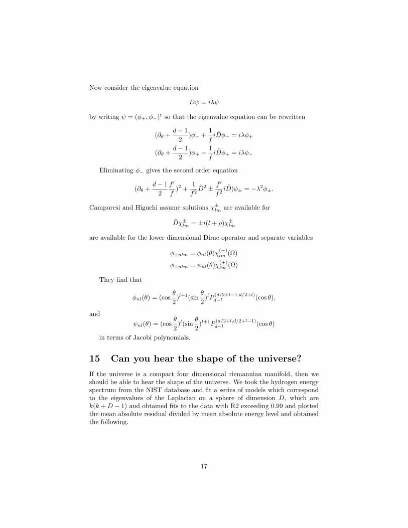
Now consider the eigenvalue equation

Dψ = iλψ

by writing ψ = (φ+, φ−)t so that the eigenvalue equation can be rewritten

(∂θ +d− 1

2)φ− +

1

fiDφ− = iλφ+

(∂θ +d− 1

2)φ+ −

1

fiDφ+ = iλφ−

Eliminating φ− gives the second order equation

(∂θ +d− 1

2

f ′

f)2 +

1

f2D2 ± f ′

f2iD)φ± = −λ2φ±.

Camporesi and Higuchi assume solutions χ±lm are available for

Dχ±lm = ±i(l + ρ)χ±lm

are available for the lower dimensional Dirac operator and separate variables

φ+nlm = φnl(θ)χ(−)lm (Ω)

φ+nlm = ψnl(θ)χ(+)lm (Ω)

They find that

φnl(θ) = (cosθ

2)l+1(sin

θ

2)lP

(d/2+l−1,d/2+l)d−l (cos θ),

and

ψnl(θ) = (cosθ

2)l(sin

θ

2)l+1P

(d/2+l,d/2+l−1)d−l (cos θ)

in terms of Jacobi polynomials.

15 Can you hear the shape of the universe?

If the universe is a compact four dimensional riemannian manifold, then weshould be able to hear the shape of the universe. We took the hydrogen energyspectrum from the NIST database and fit a series of models which correspondto the eigenvalues of the Laplacian on a sphere of dimension D, which arek(k +D − 1) and obtained fits to the data with R2 exceeding 0.99 and plottedthe mean absolute residual divided by mean absolute energy level and obtainedthe following.

17

The fits were by linear models:

AD : En = a+ b(1/SD(n)− 1/SD(n+ 1))

where SD(n) = n(n + D − 1) which are the eigenvalues of the Laplacian ona D-dimensional sphere. From the plot it is clear that among the sphericalharmonics models of different dimensions, the fit by that of dimension 4 is thebest.

16 Implications of the shape of the universe be-ing a four dimensional sphere of radius O(1/h)

A sphere has the property that every geodesic is a great circle of fixed length.This implies that only possible wavelengths are 2πR/N for integral N , andtherefore only possible frequencies are integral multiples of c/2πR where c isthe speed of light. Therefore one does not require a quantum hypothesis forquantization of energy if E = hν holds.

Another important feature of a four dimensional sphere is that there are nononzero spinors satisfying Dψ = 0 where D is the Dirac operator. This factfollows from a fairly standard argument of applying the Weitzenbock formula

D2 = ∇∗∇+ C(K)

where C(K) is a universal constant multiple of the scalar curvature which isnonnegative in this case. This implies that there are no massless fermions of afour dimensional sphere.

18

The natural electromagnetism on the four dimensional sphere is SU(2) elec-tromagnetism as the four sphere is identical to the the quaternionic projectiveline and the projection H2 → S4 restricted to pairs of quaternions with unitnorm is the Hopf fibration with fiber SU(2). If we accept the Einstein equa-tions as providing a description of gravity, then the unification of gravity andelectromagnetism amounts to providing a coherent electromagnetism via con-nections on this Hopf fibration satisfying the generalized Maxwell’s equations.

In the 1970s Sir Michael Atiyah and others have studied electromagnetismon a four dimensional sphere for mathematical interests, and Atiyah, Drinfeld,Hitchin, and Manin had constructed solutions of instanton equations.

17 Gauge theories for forces

The gravitational field equations for hree dimensional physical universe we canidentify with the Ricci curvature equation for the submanifold as in ((2)) andfollowing Yang and Mills we can recast electromagnetism and other forces viagauge theory. The following explanatory material is taken from 1999 notes byG. Svetlichny and a 1992 paper of D. Gross describing Yang Mills theory. Thecurrently accepted Standard Model contains three dynamical subtheories forquantum electrodynamics, quantum chromodynamics and electroweak theory allbased on the gauge principle, that a theory should be invariant under local phasetransformations. Note that neither this principle nor gauge theory generallyrestricts the base space of the universe, although the accepted Standard modelis based on a flat three dimensional base space. Therefore the two questionsof fundamental interest are: can we recover the results of the Standard Modelif the base space is changed to a four-sphere, and whether the geometry of afour-sphere simplifies to a classical theory.

The first gauge theory is classical Maxwell electromagnetism. In appropriatephysical units the Maxwell’s equations are:

∇ ·B = 0

∇× E +∂B

∂t= 0

∇ · E = ρ

∇×B − ∂E

∂t= J

From the homogeneous Maxwell’s equations we conclude that there is functionV called the scalar potential and a vector field A called the vector potential suchthat B = ∇×A and E = −∇V − ∂A/∂t. Consider the differential 1-form A =−V dt+Axdx+Aydy+Azdz. A direct calculation of the field strength F = dAgives the coefficients Fµν . The homogeneous Maxwell’s equations are dF = 0and for the inhomogeneous ones, one introduces j = −ρdt+Jxdx+Jydy+Jzdzand the inhomogeneous Maxwell’s equations are δF = ∗d ∗ F = j.

Recall that C. N. Yang and R. Mills introduced nonabelian gauge theoriesin the 1950s partly as a solution to understanding the surge of discoveries in

19

particle physics at the time. We can reformulate Maxwell’s electromagnetismin terms of the electromagnetic potential Aµ and the electromagnetic field Fµν .The standard formulation of Maxwell’s equations produces an abelian U(1)gauge theory. Yang and Mills produce the mechanism for a nonabelian gaugetheory where the potential Bµ that is a matrix

Bµ =1

2σaB

aµ

where σa are Pauli matrices. The differences from the abelian case of potentialAµ is that the field strength

Fµν = ∂µAν − ∂νAµ

is replaced byFµν = ∂µBν − ∂νBµ + ig[Bµ, Bν ]

Such gauge theories for forces are possible on arbitrary geometric manifoldsmathematically by considering a potential to be a connection on a principalG-bundle and considering the curvature of the connection to be identical to thefield strength.

John Preskill’s Caltech course notes for nonabelian gauge theory providesus with some of the basic issues regarding nonabelian gauge theories. We areinterested in gauge theories on a fixed compact manifold, but the basic issues arenot different from the standard treatment in the case of a noncompact universe.The minimal coupling prescription is an algorithm to promote a global U(1)symmetry to a local U(1) symmetry. In that case, one replaces ∂µφ with Dµφwhere Dµ = ∂µ − igAµ, and the local transformation are

Aµ → Aµ + ∂µω(x)

φ(x)→ exp(−ieω(x))φ(x)

In the nonabelian case SU(2) we may write an infinitesimal transformation as

Ω−1 = 1− igωaT a

where T a = 12σ

a in terms of Pauli matrices σa. Then consider the local trans-formation

q(x)→ (1− ieω(x))q(x)

under which∂µq(x)→ (1− ieω(x))∂µq − ie∂µω(x)q(x).

In order to construct an invariant Lagrangian we need to cancel the secondterm by some means. Consider Aµ(x) = Aaµ(x)T a hermitian and traceless andconsider Dµ = ∂µ − ieAµ with the transformation above leads to

Dµq → (1− igω)Dµq + ig([Dµ, ω] + δAµ)q

20

and the Dµq transforms nicely if the second term vanishes or

δAµ = [Dµ, ω] = ∂µω + ig[Aµ, ω]

Under SU(2) transformations, we have

q → Ω−1q

igAµ → Ω−1igAµΩ− (dΩ−1)Ω

Dµq → Ω−1Dµq

Fµν → Ω−1FµνΩ

Purely mathematical study of Yang-Mills theory had led to the results forwhich Simon Donaldson had received his Fields Medals, which are far outsidethe scope of this note. We can follow T. H. Parker’s study of gauge theories asclassical field theories in four dimensions in order to introduce the correspon-dence between the physical concepts and their mathematical representations. Aconnection A on a principal bundle P over a riemannian four manifold M is aYang-Mills connection when it is a critical point of the functional

A→∫M

|FA|2

Such connections are representatives of forces. The particles are represented bysections ϕ of an associated vector bundle with the action

S(A,ϕ) =

∫M

|FA|2 + |DAϕ|2 −m2|ϕ|2,

where m is the mass of the particle. T. H. Parker [7] extends a seminal resultof K. Uhlenbeck who had shown that the Yang-Mills fields cannot have isolatedsingularities to coupled Yang-Mills equations, both for fermions, based on theDirac operator acting on bundle-valued spinors and for bosons based on thebundle Laplacian. Thus for compact orientable riemannian manifolds gaugetheory has been studied and the mathematical framework exists with reasonableresults. The central issue of this note is to point out the evidence that the actualphysical universe could be described by this mathematical formalism.

In details taken from T. Parker, let pi : P → M be a principal bundle withcompact structure group G and ρ : G → Aut(V ) be a unitary respresentationwith associated vector bundle E = P ×ρ V and let W be any bundle associatedto the frame bundle of M . Let M be the set of metrics on M , let A be theconnections on P and let E = −(E ⊗W) so that we can write an action

S(g,A, φ) =

∫M

L(g,A, φ)

for L a 4-form constructed from g, A and φ. An automorphism f of P is a mapfor which f(xg−1) = f(x)g−1. The subgroup of orientation preserving automor-phisms that project to the identity map on M can be identified with P ×Ad G,

21

and these automorphisms are called gauge transformations G. The Killing formprovides an invariant metric h on the adjoint bundle and a hermitian metricon E.

Consider Lagrangians L with the properties of regularity – that in local co-ordinates L should be a universal polynomial in g, h, Γ (the Christoffel symbolsof A), (det g)−1/2, (deth)−1/2 and their derivatives; naturality under bundleautomorphism f and conformal invariance. Then invariant theory can be usedto determine the possibilities for L. Naturality under orientation preservingdiffeomorphisms of P implies, by SO(4) invariant theory that

L = a1|s|2 + a2|B|2 + a3|W+|2 + a4|W−|2 + a5Ω ∧ Ω + a6Ω ∧ ∗Ω,

The Yang-Mills action is

S(g,A) =

∫M

Ω ∧ ∗Ω.

The space of connections A carries a natural differentiable structure on whichthis is a smooth function, and whose critical points are Yang-Mills fields. In thevector bundle formalism, if E is a vector bundle associated to P by a locallyfaithful orthogonal representation of G, each connection on P corresponds to adifferential operator ∇ : Γ(E)→ Γ(Λ1 ⊗ E) where

∇(fϕ) = df ⊗ ϕ+ f ⊗∇ϕ

The curvature field

ΩX,Y = ∇X∇Y −∇Y∇X −∇[X,Y ]

is a two form with values in the skew symmetric endomorphism of E. The normof Ω at a point x is given by

‖Ω‖2 =∑i<j

‖Ωei,ej‖2

where (e1, . . . , en) is an orthonormal frame, and the inner product on skewsymmetric endomorphisms of E is

〈A,B〉 = −1/2 trace(A B)

For any bundle with connection F , there is a sequence of differential operatorsd∇ : Γ(Λp ⊗ F )→ Γ(Λp+1 ⊗ F ) given by

(d∇ϕ)(X0, . . . , Xp) =

p∑k=0

(−1)k(∇Xkϕ)(X0, . . . , Xk, . . . , Xp).

We can define adjoints δ∇ using the formula

(δ∇ϕ)(X1, . . . , Xp) = −n∑k=1

(∇ekϕ)(ek, X1, . . . , Xp)

22

The first variation formula for the Yang Mills functional shows that ∇ is acritical point if and only if δ∇Ω = 0, which because of the Bianchi identityd∇Ω = 0 is equivalent to ∆∇Ω = 0 where ∆∇ = d∇δ∇ + δ∇d∇.

For four dimensional base space, two-forms break up by the eigenspaces ofthe ∗-operator. Then Ω = Ω+ + Ω− is harmonic if and only if both componentsare harmonic. Bourgaignon, Lawson and Simon show that on a four spherewhen G is SU(2) or SU(3) any weakly stable Yang-Mills field is either self-dualor anti-self-dual.

In this setting we have the coupled fermion equations

(d∇)∗Ω = −1/2∑〈ϕ, ei · ρ(σα)ϕ〉σα ⊗ ei

Dϕ = mϕ

and the coupled boson equations

(d∇)∗Ω = J = −<∑〈∇iϕ, ρ(σα)ϕ〉σα ⊗ ei

∇∗∇ϕ = (s/6)ϕ+ a|ϕ|2ϕ+m2ϕ.

18 The zero modes and lower bound of the firsteigenvalue of a twisted Dirac

On general four dimensional spin manifolds one has the Dirac operator onspinors via the Spin connection. When the scalar curvature is positive, thisDirac operator has zero kernel. On the other hand, one can consider a self dualconnection A on an auxiliary principal G-bundle P and using a unitary repre-sentation of G on a complex vector bundle E consider the covariant derivative∇A. The twisted Dirac operator is then DA : Γ(V ⊗ E) → Γ(V ⊗ E) which is∇ = ∇S ⊗ 1 + 1 ⊗ ∇A followed by clifford multiplication. This twisted Diracoperator has kernel dimension dictated by the topology of E and

dim kerDA =1

2p1(E)

This is not generally zero even on a four sphere which has constant positivescalar curvature. Atiyah, Hitchin Singer give a Weitzenbock formula and showthat when A is selfdual, M is selfdual and has positive scalar curvature thenone can show vanishing of ψ with DAψ = 0. Helga Baum has shown that thefirst eigenvalue of the twisted Dirac operator for positive scalar curvature fourmanifold satisfies

λ1 ≥√R0/3

and that this On a four sphere universe this provides a gap between the zeroand the first eigenvalue for the twisted Dirac operator, which translates to amass gap that does not translate to R4. This is an interesting observationas the question of mass gap for nonabelian gauge theories has remained open.This lower bound due to Helga Baum and implicit in Atiyah-Hitchin-Singer

23

is geometric rather than topological. On the other hand, there is a positivedimensional kernel, so for S4 we have a fairly clear answer for the question ofthe twisted Dirac spectrum.

The mechanism for nonabelian gauge theories translates without problems toa fixed spherical space. The Standard Model is a U(1)× SU(2)× SU(3) gaugetheory that was successful in uniting the nuclear and electromagnetic forcesby 1973. But knowledge that the universe is a four dimensional stationarysphere allows us to re-examine whether electromagnetism itself is an SU(2)gauge theory and thus conjecture that there are further simplifications possible,such as realizing that since a classical electron orbiting a classical proton in fourdimensions need not be unstable, and therefore it is possible to seek a singleforce governing nature which are thought to be separate in the nuclear forces.

In the case where the space manifold is the four-sphere, we have a naturalprincipal SU(2)-bundle which is the Hopf fibration S7 → S4. It is natural toask what the relation is between electromagnetism in the material universe,which we can identify with a three-dimensional submanifold M which fromthe electromagnetic theory developed from Maxwell, we consider to have U(1)symmetry, to SU(2) electromagnetism that can be said to arise naturally fromthe Hopf fibration.

19 The Standard Model in a 4-sphere universe

The Kaluza-Klein theories led to work on adapting the Standard Model to higherdimensions. An example of this approach is the one used by Pomarol and Quirosfrom 1998 [8]. In the Kaluza-Klein case the base space of the universe is a threedimensional manifold with the extra dimension compactified to S1/Z2, so aproduct structure. In this case the product structure allows one to expand fieldsby Fourier series in the extra dimension. This cannot be done for submanifoldsof S4 directly but in this case too the normal vector field picks out a great circlegeodesic and so we have a natural circle-bundle structure for M . Thus we canmodify Pomarol-Quiros technique of showing how to obtain the Standard Modelas a reduction of a higher dimensional theory where we must systematicallyreplace the global Fourier series by a different method of combining M with theextra dimension. For generic points on M embedded in an S4 the intersectionof the normal circle with M has a finite number of points. Intuitively, one needsa Fourier series expansion along the circle with a finite number of points whosevalues are fixed. Thus the reduction to the Standard Model is the Pomarol-Quiros analysis modified with Fourier series with constraints. The qualitativeresult is the same as for the Kaluza-Klein case – i.e. higher dimensional theorycan restrict to the Standard Model on M .

In five (including time) dimensions, the vector supermultiplet (VM , λiL,Σ) of

an SU(N) gauge theory consists of a vector boson VM a real scalar Σ and twobispinors λiL all in the adjoint representation of SU(N). The 5D Lagrangian is

24

given by

L =1

g2trace−1

2F 2MN + |DMΣ|2 + iλiγMDMλ

i − λi[Σ, λi], (4)

where λi is the symplectic-Majorana spinor (λiL, εij λjL)T . The 5D matter su-

permultiplet (Hi,Ψ) consists of two scalar fieds Hi and a Dirac spinor Ψ =(ΨL,ΨR)T . The Lagrangian for the matter supermultiplets interacting withthe vector supermultiplet is given by

L = |DMHai |2 + iΨaγ

MΨa + hc)− ΨaΣΨa

− HiaΣ2Ha

i −g2

2

∑m,α

[Hiα(σm)jiT

αHaj ]2,

where σ are Pauli matrices.Since all the interactions in these Lagrangians are gauge interactions the

model based on the Standard Model gauge group GSM = SU(3) × SU(2) ×U(1) is easily constructed from these expressions. It contains vector multipletsin the adjoint representation of GSM and two Higgs hypermultiplets in therepresentation [(1, 2, 1/2) + (1, 2,−1/2)]. The chiral matter is located on theboundary M and contains the usual chiral N = 1 three dimensional multiplets.

19.1 Modifications of Pomarol-Quiros for hypersurfaces ofspheres

The main issue is to find a replacement for the Fourier series expansion. In thiscase we can translate the Fourier expansion, with x being coordinates on thehypersurface and y coordinates along the normal geodesic

Φ(x, y) =∑k

Φk(x)Pk(cosy/R)

where Pk is the k-th Gegenbauer polynomial with α = 3/2. This decompositionarises from a spherical harmonic expansion and considering y as the angle ofrotation that fixes a ’pole’ on the sphere such that the rotation draws out y.While the mass spectra in the Kaluza-Klein excitations are k/R, in this case themass spectrum is

√k(k + 3)/R corresponding to the eigenvalues of the spher-

ical harmonics. For the Pomarol-Quiros arguments for a reduction to a threedimensional Standard Model, the quantitative difference in the mass spectrumproduces no difficulties.

20 Electromagnetism on quaternionic Kahler man-ifolds

In the last section, we showed a path to recover the Standard Model on athree dimensional ’physical’ universe of a four dimensional sphere. But the four

25

dimensional sphere is the quaternionic projective line. It is possible to argue forthe naturality of the electromagnetic duality through the geometry for examplevia the setup of Kramers, Semmelmann and Weingart [2]. The idea is to explorepossibilities of a fundamental deterministic physical theory that might be able toexplain observations as well or better than a quantum mechanics based physics.We note that the spinors are providing the square root of the wave equation withthe spin representations decoupling electric and magnetic fields. The source freeMaxwell’s equations are being solved with the Dirac operator replacing curl. Inother words there is a naturality to electromagnetism in this case that arise inthis case where SO(4) = Sp(1) · Sp(1).

We follow exactly the preliminaries of Kramer, Semmelmann and Weingartwithout novelty and then consider the question of the naturality of electromag-netism in our actual universe. The symplectic form defines an isomorphism] : E → E∗, e] = σE(e, ·) with inverse [ : E∗ → E. Using Gram’s determinantor permanent the symplectic form σE can be extended to

∧sE or Symr E. The

extension satisfiesσE(e ∧ η1, η2) = σE(η1, e

]yη2)

The holonomy group of S4 is exactly Sp(1) · Sp(1) = SU(2) · SU(2) but theformalism of quaternionic Kahler manifolds, whose holonomies reduce to Sp(d) ·Sp(1) ⊂ SO(4d) is useful for context. If P is the frame bundle reduced, thenany representation V of Sp(d)× Sp(1) gives a local vector bundle V associatedto P that extends globally if the representation factors through Sp(d) · Sp(1).Let H and E be the defining complex representations of Sp(1) and Sp(d) with

invariant symplectic forms σH ∈∧2

H∗ and σE ∈∧2

E∗ and theit positivequaternionic structures J so σE(Je1, Je2) = ¯σE(e1, e2). The symplectic formσE can be expended to the exterior and symmetric powers of E and satisfy

σE(e ∧ η1, η2) = σE(η1, e]yη2).

Analogous constructions are true for H. For bases ei and dei of E and E∗ then

σE =1

2

∑de1 ∧ e]iLE =

1

2

∑de[i ∧ ei.

Wedging with LE defines homomorphism L :∧k−2

E →∧k

E whereas contract-ing with σE defines its adjoint Λ. The operators L,Λ and H = [L,Λ] followthe commutator rules of sl2C. Therefore ΛkE = im(L) + ker(Λ) as an Sp(n)

representation and the primitive space∧k

0 E = ker(Λ) is irreducible. One hasthe decomposition

q∧E =

[q/2]⊕k=0

q−2k∧0

E.

Contraction with elements of E∗ preserves the primitive spaces, and the projec-tion of wedge e ∧ ω to

∧q0E, denoted e ∧0 ω is given by

e ∧0 ω = e ∧ ω − 1

d− k + 1LE ∧ (e]yω).

26

By the Peter-Weyl theorem any irreducible Sp(d) × Sp(1)-module can berealized as a subspace of tensor products H⊗p ⊗ E⊗q for some p and q. Henceany vector bundle associated to P can be expressed in terms of H and E. Forexample, the complexified tangent space is

TMC = H ⊗ E.

The spinor bundle of a quaternionic Kahler manifold decomposes as

S(M) =

d⊕r=0

Sr(M) = ⊕r=0 SymrH ⊗d−r∧

0

E

and for any tangent vector h ⊗ e ∈ H ⊗ E0TM , the Clifford multiplication isgiven by c(h⊗ e) =

√2(h · ⊗e]y + h]y0 ⊗ e∧0).

21 Quaternion projective spaces in complex ma-trices

Following Furutani and Tanaka, who provided a Khler structure on the punc-tured cotangent bundle on quaternionic projective spaces, we can embed generalquaternionic projective spaces PnH into spaces of complex matrices as follows.

Let ρ : H→M(2,C) be the representation given by

ρ(p) = ρ(z + wj) =z w−w z

(5)

Introduce a metric on PnH via the Hopf fibration π : S4n+3 → PnH wherep→ [p] for p = (p0, . . . , pn) ∈ Hn. The embedding of PnH into M(2n+ 2,C) isgiven by

[p]→ (Pij) = (ρ(pipj))

The image of this embedding consists of P ∈ M(2n + 2,C) satisfying P 2 =P, P ∗ = P, trace(P ) = 2, PJ = J tP . The canonical one-form can be written as

θPnH(P,Q) =1

2(dPH)∗ trace(QdP )

and so the symplectic form can be written

ωPnH =1

2(dPH)∗ trace(dQ ∧ dP ).

The symplectic form allows us to specify classical mechanics on quaternionicprojective spaces and we may focus attention to the case of P 1H = S4.

27

References

[1] N. G. de Bruijn, Algebraic theory of penrose’s non-periodic tilings of theplane, i, ii, Indagaciones mathematicae 43 (1981), no. 1, 39–66.

[2] Semmelmann U. Kramer, W. and Weingard G., Eigenvalue estimates forthe dirac operator on quaternionic kahler manifolds, Math. Z. 230 (1999),no. 4, 727–751.

[3] M-A Lawn and J. Roth, Isometric immersion of hypersurfaces in 4-dimensional manifolds via spinors, (2008).

[4] P. Li and S-T. Yau, On the parabolic kernel of the schroedinger operator,Acta Mathematica 156.

[5] Croft C. M. Lee R. H. Lolley, R. N., Photoreceptors of the retina andpinealocytes of the pineal gland share common components of signal trans-duction, Neurochem Res. 17 (1992), no. 1, 81–9.

[6] Freedman M. S. Soni B. M. Munoz M Garcia-Fernandex J-M. Foster R.Lucas, R. J.

[7] Thomas H. Parker, Gauge theories on four dimensional riemannian mani-folds, Comm. Math. Phys. 85, 563–602.

[8] A. Pomarol and M. Quiros.

[9] L. Randall and R. Sundrum, An alternative to compactification,http://arxiv.org/abs/hep-th/9906064 (1999).

[10] R. Vaidyanathaswamy, Integer-roots of the unit matrix, J. London Math.Soc. s1-3, no. 2, 121–124.

[11] Pei Wang, Kaluza-klein dimensional reduction and gauss-codazzi-ricci equa-tions, http://arxiv.org/abs/0805.4479.

[12] P. S. Wesson and Ponce de Leon, Kaluza-klein equations, einstein’s equa-tions, and the effective energy-momentum tensor, J. Math. Phys. 33 (1992),no. 3883.

[13] Fritz Zwicky, On the red shift of spectral lines through intersteller space,Proceedings of the National Academy of Sciences (1929).

28